Mixing conditions of conjugate processes

Abstract

We give sufficient conditions ensuring that a $\psi$–mixing property holds for the sequence of empirical cdfs associated to a conjugate process.

and

a]Instituto de Matemática e Estatística – Universidade Federal do Rio Grande do Sul

1 Introduction

In Horta and Ziegelmann (2018) a conjugate process is defined to be a pair $(\xi,\,X)$, where $X\coloneqq(X_{\tau}:\,\tau\geq 0)$ is a real valued, continuous time stochastic process, and $\xi\coloneqq(\xi_{t}:\,t=0,1,\dots)$ is a strictly stationary sequence of $M_{1}(\mathbb{R})$-valued random elements, for which the following condition holds:

$$\mathbb{P}\left(X_{\tau}\in B\,|\,\xi_{0},\xi_{1},\dots\right)=\xi_{t}\left(B\right),\qquad\tau\in\left[t,t+1\right),$$ (1.1)

for each $t=0,1,\dots$ and each Borel set $B$ in the real line. From the statistical viewpoint, the sequence $\xi$ is to be understood as a latent (i.e. unobservable) process, and thus all inference must be carried using information attainable from the continuous time, observable process $X$ alone. A crucial objective in this context is estimation of the operator $R^{\mu}\colon L^{2}\left(\mu\right)\rightarrow L^{2}\left(\mu\right)$ defined by

$$R^{\mu}f\left(x\right)\coloneqq\int R_{\mu}\left(x,y\right)f\left(y\right)\,\mu\left(\mathrm{d}y\right),\qquad x\in\mathbb{R}$$ (1.2)

where the kernel $R_{\mu}$ is given by

$$R_{\mu}\left(x,y\right)\coloneqq\int\operatorname*{Cov}\left(F_{0}\left(x\right),F_{1}\left(z\right)\right)\operatorname*{Cov}\left(F_{0}\left(y\right),F_{1}\left(z\right)\right)\,\mu\left(\mathrm{d}z\right),\qquad x,y\in\mathbb{R},$$

and where $\mu$ is a fixed, arbitrary probability measure on $\mathbb{R}$ equivalent to Lebesgue measure. In the above, $F_{t}\left(x\right)\coloneqq\xi_{t}\left(-\infty,x\right]$, $x\in\mathbb{R}$, is the (random) cdf corresponding to $\xi_{t}$.

One of the key results in Horta and Ziegelmann (2018) is Theorem 1 below, which provides sufficient conditions under which $R^{\mu}$ can be $\sqrt{n}$-consistently estimated. Before stating the theorem, we shall shortly introduce the estimator $\widehat{R}^{\mu}$ which is (as one should expect) a sample analogue of $R^{\mu}$. Consider, for each $t=1,\dots,n$, a sample of observations $\left\{X_{i,t}:\,i=1,\dots,q_{t}\right\}$ of size $q_{t}$ from $\left(X_{\tau}:\,\tau\in\left[t,t+1\right)\right)$. Typically one has $X_{i,t}=X_{t+(i-1)/q_{t}}$. We then let $\widehat{F}_{t}$ denote the empirical cdf associated with the sample $X_{1,t},\dots,X_{q_{t},t}$,

$$\widehat{F}_{t}(x)\coloneqq\frac{1}{q_{t}}\sum_{i=1}^{q_{t}}\mathbb{I}[X_{i,t}\leq x],\qquad x\in\mathbb{R}.$$

Notice that both $F_{t}$ and $\widehat{F}_{t}$ are random elements with values in the Hilbert space $L^{2}(\mu)$, and thus we find ourselves in a framework similar to Horta and Ziegelmann (2016).

In this setting, $\widehat{R}^{\mu}$ is defined to be the operator acting on $L^{2}\left(\mu\right)$ with kernel

$$\widehat{R}_{\mu}\left(x,y\right)\coloneqq\int\widehat{C}_{1}\left(x,z\right)\widehat{C}_{1}\left(y,z\right)\mu\left(\mathrm{d}z\right),\qquad x,y\in\mathbb{R},$$

where $\widehat{C}_{1}$ is the sample lag-1 covariance function

$$\widehat{C}_{1}\left(x,y\right)\coloneqq\frac{1}{n-1}\sum_{t=1}^{n-1}\left(\widehat{F}_{t}\left(x\right)-\bar{F}_{0}\left(x\right)\right)\times\left(\widehat{F}_{t+1}\left(y\right)-\bar{F}_{0}\left(y\right)\right),\qquad x,y\in\mathbb{R},$$

with $\bar{F}_{0}\coloneqq\left(1/n\right)\sum_{t=1}^{n}\widehat{F}_{t}$.

Last but not least, let $X^{(t)}$ denote the stochastic process $\left(X_{t+\tau}:\,\tau\in\left[0,1\right)\right)$, so that $X^{(0)},X^{(1)},\dots,X^{(t)},\dots$ is a sequence of $\mathbb{R}^{[0,1)}$-valued random elements. We say that a conjugate process $\left(\xi,\,X\right)$ is cyclic independent if, conditional on $\xi$, we have that $\left(X^{(t)}:\,t=0,1,\dots\right)$ is an independent sequence. This means that, for each $n$ and each $(n+1)$-tuple $\mathcal{C}_{0},\dots,\mathcal{C}_{n}$ of measurable subsets of $\mathbb{R}^{[0,1)}$, it holds that

$$\mathbb{P}(X^{(0)}\in\mathcal{C}_{0},\dots,X^{(n)}\in\mathcal{C}_{n}\,|\,\xi)=\prod_{t=0}^{n}\mathbb{P}(X^{(t)}\in\mathcal{C}_{t}\,|\,\xi).$$ (1.3)

We are now ready to state the consistency theorem.

Theorem 1 (Horta and Ziegelmann (2018)).

Let $\left(\xi,X\right)$ be a cyclic–independent conjugate process, and let $\mu$ be a probability measure on $\mathbb{R}$ equivalent to Lebesgue measure. Assume that $\big{(}\widehat{F}_{t}\colon\,t=1,2,\dots\big{)}$ is a $\psi$–mixing sequence, with the mixing coefficients $\Psi\left(k\right)$ satisfying $\sum_{k=1}^{\infty}k\,\Psi^{1/2}\left(k\right)<\infty$. Then it holds that

1. $\|\widehat{R}^{\mu}-R^{\mu}\|_{HS}=O_{\mathbb{P}}\left(n^{-1/2}\right)$;

2. $\sup_{j\in\mathbb{N}}|\widehat{\theta}_{j}-\theta_{j}|=O_{\mathbb{P}}\left(n^{-1/2}\right)$.

If moreover the nonzero eigenvalues of $R^{\mu}$ are all distinct, then

1. $\|\widehat{\psi}_{j}-\psi_{j}\|_{L^{2}(\mu)}=O_{\mathbb{P}}\big{(}n^{-1/2}\big{)}$, for each $j$ such that $\theta_{j}>0$.

In the above, $\|\cdot\|_{HS}$ denotes the Hilbert-Schmidt norm of an (suitable) operator acting on $L^{2}(\mu)$, $(\theta_{j}\colon\,j\in\mathbb{N})$ (resp. $(\widehat{\theta}_{j}\colon\,j\in\mathbb{N})$) denotes the non-increasing sequence of eigenvalues of $R^{\mu}$ (resp. $\widehat{R}^{\mu}$), with repetitions if any, and, for $j\in\mathbb{N}$, $\psi_{j}$ (resp. $\widehat{\psi}_{j}$) denotes the unique eigenfunction associated with $\theta_{j}$ (resp. $\widehat{\theta}_{j}$).

2 Main result

In what follows it will be convenient to assume that the latent process is indexed for $t\in\mathbb{Z}$ and that the continuous time, observable process $X$ is indexed for $\tau\in\mathbb{R}$. That is, we update our definitions so that $\xi\coloneqq(\xi_{t}:\,t\in\mathbb{Z})$ and $X\coloneqq(X_{\tau}:\,\tau\in\mathbb{R})$. Recall (see Bradley (2005)) that a strictly stationary sequence $(Z_{t}:t\in\mathbb{Z})$ of random elements taking values in a measurable space $\mathcal{Z}$ is said to be $\psi$-mixing if the $\psi$-mixing coefficient $\Psi_{Z}$ defined, for $k\in\mathbb{N}$, by

$$\Psi_{Z}(k)\coloneqq\sup\left|1-\frac{\mathbb{P}(A\cap B)}{\mathbb{P}(A)\mathbb{P}(B)}\right|$$ (2.1)

is such that $\Psi_{Z}(k)\to 0$ as $k\to\infty$, where the supremum in (2.1) ranges over all $A\in\sigma(Z_{t}\colon\,t\leq 0)$ and all $B\in\sigma(Z_{t}\colon\,t\geq k)$ for which $\mathbb{P}(A)\mathbb{P}(B)>0$.

The $\psi$–mixing condition in Theorem 1 imposes restrictions on the sequence of empirical cdfs $\big{(}\widehat{F}_{t}\big{)}$ and thus constrains $(F_{t})$ and $(X_{\tau})$ jointly. One could argue that it is more natural to impose a $\psi$–mixing condition on the latent process $(\xi_{t})$ instead, the issue being that it may be the case that a mixing property of the latter sequence is not inherited by $(\widehat{F}_{t})$. If a condition slightly stronger than cyclic–independence is imposed, however, then inheritance does hold. This is our main result.

Theorem 2.

Let $\left(\xi,\,X\right)$ be a cyclic–independent conjugate process, and let $\mu$ be a probability measure on $\mathbb{R}$ equivalent to Lebesgue measure. Assume $\xi$ is $\psi$–mixing with mixing coefficient sequence $\Psi_{\xi}$. If, for each $t$, the conditional distribution of $X^{\left(t\right)}$ given $\xi$ depends only on $\xi_{t}$, in the sense that the equality

$$\mathbb{P}\big{[}X^{\left(t\right)}\in\mathcal{C}\,\big{|}\,\xi\big{]}=\mathbb{P}\big{[}X^{\left(t\right)}\in\mathcal{C}\,\big{|}\,\xi_{t}\big{]}$$ (2.2)

holds for each measurable subset $\mathcal{C}$ of $\mathbb{R}^{\left[0,1\right)}$ and each $t$, then $\big{(}X^{\left(t\right)}\big{)}$ is $\psi$–mixing with mixing coefficient sequence $\Psi_{X}\leq\Psi_{\xi}$.

Corollary 1.

In the conditions of Theorem 2, if $\sum_{k=1}^{\infty}k\Psi_{\xi}(k)^{1/2}<\infty$, then the $\psi$–mixing assumption of Theorem 1 holds.

Proof of Theorem 2.

For $k\in\mathbb{N}$, let $T_{1}$ and $T_{2}$ be finite, nonempty subsets of $\{0,-1,-2,\dots\}$ and $\{k,k+1,k+2,\dots\}$ respectively, and set $T_{0}\coloneqq T_{1}\cup T_{2}$. Let $\{\mathcal{C}_{t}$, $t\in T_{0}\}$ be a collection of measurable subsets of $\mathbb{R}^{\left[0,1\right)}$. By definition, $\sigma(X^{(t)}:\,t\leq 0)$ coincides with the $\sigma$-field generated by the class of sets of the form $\bigcap_{t\in T_{1}}[X^{(t)}\in\mathcal{C}_{t}]$ over all finite, nonempty $T_{1}\subset\{0,-1,-2,\dots\}$ and all collections $\{\mathcal{C}_{t}:\,t\in T_{1}\}$ of measurable subsets of $\mathbb{R}^{[0,1)}$, and similarly for $\sigma(X^{(t)}:\,t\geq k)$.

Notice that by equation (2.2) and the Doob–Dynkin Lemma (see (Kallenberg, 1997, Lemma 1.13)) we have $\mathbb{P}\left[X^{\left(t\right)}\in\mathcal{C}_{t}\,|\,\xi\right]=g_{t}\circ\xi_{t}$, for some measurable function $g_{t}\colon M_{1}\left(\mathbb{R}\right)\rightarrow\mathbb{R}$. This fact, together with the cyclic–independence assumption, ensures that

$$\mathbb{P}\left\{\bigcap_{t\in T_{j}}\left[X^{\left(t\right)}\in\mathcal{C}_{t}\right]\right\}=\mathbb{E}\left\{\mathbb{P}\left\{\bigcap_{t\in T_{j}}\left[X^{\left(t\right)}\in\mathcal{C}_{t}\right]\,\Big{|}\,\xi\right\}\right\}=\mathbb{E}\left\{\prod_{t\in T_{j}}g_{t}\circ\xi_{t}\right\},$$

$j=0,1,2$ (a similar computation yields strict stationarity of the process $(X^{(t)}:\,t\in\mathbb{Z})$). Thus, the quantity

$$\left|1-\frac{\mathbb{P}\left\{\bigcap_{t\in T_{0}}\left[X^{\left(t\right)}\in\mathcal{C}_{t}\right]\right\}}{\mathbb{P}\left\{\bigcap_{t\in T_{1}}\left[X^{\left(t\right)}\in\mathcal{C}_{t}\right]\right\}\mathbb{P}\left\{\bigcap_{t\in T_{2}}\left[X^{\left(t\right)}\in\mathcal{C}_{t}\right]\right\}}\right|$$ (2.3)

is seen to be equal to

$$\left|1-\frac{\mathbb{E}\left\{\prod_{t\in T_{0}}g_{t}\circ\xi_{t}\right\}}{\mathbb{E}\left\{\prod_{t\in T_{1}}g_{t}\circ\xi_{t}\right\}\mathbb{E}\left\{\prod_{t\in T_{2}}g_{t}\circ\xi_{t}\right\}}\right|.$$ (2.4)

Substituting each $g_{t}$ in (2.4) by an arbitrary measurable, bounded and positive $g_{t}^{\prime}\colon M_{1}\left(\mathbb{R}\right)\rightarrow\mathbb{R}$, and taking the supremum over all collections $\left\{g_{t}^{\prime}:\,t\in T_{0}\right\}$ of such $g_{t}^{\prime}$, and over all $T_{0}=T_{1}\cup T_{2}$ as above, gives an upper bound to (2.3). It is easily seen that this supremum yields precisely $\Psi_{\xi}\left(k\right)$. This establishes that $\Psi_{X}\left(k\right)\leq\Psi_{\xi}\left(k\right)$ and completes the proof. ∎

Proof of Corollary 1.

By definition (or using the Doob–Dynkin Lemma) we have that $\widehat{F}_{t}$ is of the form $\widehat{F}_{t}=g_{t}\circ X^{(t)}$ for some measurable $g_{t}\colon\mathbb{R}^{[0,1)}\to L^{2}(\mu)$. Since $\mathbb{P}(\widehat{F}_{t}\in B)=\mathbb{P}(X^{(t)}\in g_{t}^{-1}(B))$, it follows that the supremum in the LHS over all measurable subsets $B$ of $L^{2}(\mu)$ is bounded above by $\sup\mathbb{P}(X^{(t)}\in\mathcal{C})$, with $\mathcal{C}$ ranging over all measurable subsets of $\mathbb{R}^{[0,1)}$. An easy adaptation of this argument shows that the mixing coefficient sequence $\Psi_{\widehat{F}}$ is bounded above by $\Psi_{X}$. ∎

3 Examples

We refer the reader to Horta and Ziegelmann (2018) for an interesting application of the theory of conjugate processes to the problem of financial risk forecasting. Below we provide a simple example to illustrate the theory.

As discussed in Horta and Ziegelmann (2018), the case where $(\xi_{t})$ is an independent sequence is of no interest, since in this case $R^{\mu}$ is trivially the zero operator. Consider then an iid sequence $(\vartheta_{t}:\,t\in\mathbb{Z})$, where $\vartheta_{t}$ is uniformly distributed on $[0,1]$, and let $\eta_{t}$ be the random probability measure defined by (abusing a little on notation) $\eta_{t}(0)=\vartheta_{t}$ and $\eta_{t}(1)=1-\vartheta_{t}$. Setting $\xi_{t}\coloneqq(\eta_{t}+\eta_{t-1})/2$, we clearly obtain a $\psi$-mixing sequence which satisfies the summability condition of Theorem 1. Indeed, $(\xi_{t})$ is $1$-dependent. A straightforward computation shows that $\operatorname*{Cov}(F_{0}(x),F_{1}(y))=1/48$ for $x,y\in[0,1)$ and is identically zero otherwise, and therefore $R_{\mu}(x,y)$ is a positive constant for $x,y\in[0,1)$ which only depends on the chosen measure $\mu$.

Now, aside from the assumption that relation (1.1) holds, the nature of the process $(X_{\tau}:\,\tau\in\mathbb{R})$ is rather arbitrary. Below we simulate the case where, conditional on $\xi$, the process $(X_{t+\tau}:\,\tau\in[0,1))$ is a continuous time Markov chain on the state space $\{0,1\}$ with stationary distribution $(\xi_{t}(0),\xi_{t}(1))$. There is a free parameter in the construction, which is the mean holding time $1/q_{0}$ of state $0$. We set $q_{0}=10$. Thus, conditional on $\xi_{t}=\lambda_{t}$, the process $(X_{t+\tau}:\,\tau\in[0,1))$ is a Markov chain with initial distribution $(\lambda_{t}(0),\lambda_{t}(1))$ and generator

$$Q=\begin{pmatrix}-q_{0}&q_{0}\\ r_{t}&-r_{t}\end{pmatrix}$$

where $r_{t}\coloneqq q_{0}\lambda_{t}(0)/\lambda_{t}(1)$.

The conjugate process $(\xi,X)$ described above can be informally summarized as follows. At each day, the world finds itself in a (unobservable) state which is characterized by a number lying in $[0,1]$. Within each day, given the state of the world, a system can find itself in two distinct (observable) regimes (say, regime $\bar{0}$ and regime $\bar{1}$). This system switches between $\bar{0}$ and $\bar{1}$ according to a stationary, continuous time Markov chain, where the state of the world in that day represents the probability of the system being on regime $\bar{0}$ at any given point in time within that day. Figure 1 displays a simulated sample path for the first 4 days of the process just described.

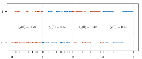
Figure 1: A simulated sample path. Even days are colored in red; odd days in blue.

We also illustrate the consistency result via a Monte Carlo simulation study. For each $t=1,\dots,n$, we sample the process $(X_{t+\tau}:\,\tau\in[0,1))$ once per cycle (that is, we take $q_{t}=1$ and $X_{1,t}=X_{t}$) and compute the corresponding value of $\widehat{C}_{1}(0,0)$. Figure 2 displays the boxplot of the estimated values of $\widehat{C}_{1}(0,0)$ across $10000$ replications of the above procedure, with the sample size varying in $\{100,1000,10000\}$. The blue line indicates the true parameter value $C_{1}(0,0)=1/48$.

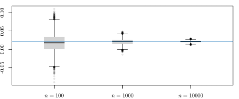
Figure 2: Boxplots of $\widehat{C}_{1}(0,0)$ values across replications.

References

• Horta and Ziegelmann (2018) Horta, E. and Ziegelmann, F. (2018) Conjugate processes: Theory and application to risk forecasting, Stochastic Processes and their Applications 128Β (3) 727–755. doi:10.1016/j.spa.2017.06.002.
• Horta and Ziegelmann (2016) Horta, E. and Ziegelmann, F. (2016) Identifying the spectral representation of Hilbertian time series, Statistics & Probability Letters 118 45–49. doi:10.1016/j.spl.2016.06.014.
• Bradley (2005) Bradley, R.Β C. (2005) Basic Properties of Strong Mixing Conditions. A Survey and Some Open Questions, Probability Surveys 2Β (0) 107–144. doi:10.1214/154957805100000104.
• Kallenberg (1997) Kallenberg, O. (1997) Foundations of Modern Probability, Probability and its Applications, Springer-Verlag, New York. doi:10.1007/b98838.