Two components of donor-acceptor recombination in compensated semiconductors. Analytical model of spectra in presence of electrostatic fluctuations

Abstract

We report numerical and analytical studies of the donor-acceptor recombination in compensated semiconductors. Our calculations take into account random electric fields of charged impurities which are important in non zero compensation case. We show that the donor-acceptor optical spectrum can be described as a sum of two components: monomolecular and bimolecular. In the low compensation limit we develop two analytical models for both types of the recombination. Also our numerical simulation predicts that these two components of the photoluminescence spectra can be resolved under certain experimental conditions.

I Introduction

The donor-acceptor (DA) optical transition is due to a tunnel recombination between distant impurity pairs Thomas et al. (1965). If radii of both impurity states are comparable with the lattice constant then the spectrum of DA recombination appears as a set of narrow lines which corresponds to discreet positions of impurities in a crystal lattice. If one of the impurity states (donor, for instance) is shallow and can be described with the hydrogen-like wave function with radius $a_{b}$ then DA recombination corresponds to a broad spectrum. The probability $p$ of the transition exponentially decreases with inter-impurity distance $r$. The photon energy $\hbar\omega$ increases due to Coulomb interaction $e^{2}/\varepsilon r$ between ionized donor and acceptor in the final state:

$$p=p_{0}\exp{\left(-\frac{2r}{a_{b}}\right)};$$ (1)

$$\hbar\omega=E_{g}-E_{d}-E_{a}+\frac{e^{2}}{\varepsilon r}.$$ (2)

Here $E_{g}$ is the bandgap of the material, $E_{d}$ and $E_{a}$ — donor and acceptor binding energies, $p_{0}$ is a part of matrix element which does not depend on a distance. For short we use the denotation $E=\hbar\omega-(E_{g}-E_{d}-E_{a})$ which we call the transition energy in the rest of the paper.

It is easy to derive the spectral dependence of the transition probability $P(E)$ Thomas et al. (1965); Osipov and Foigel (1976); Bogoslovskiy et al. (2016). The probability to find a donor at a distance $r$ from an arbitrary acceptor equals $N_{d}4\pi r^{2}dr$, where $N_{d}$ is the concentration of donors. Calculating $dr=({dr}/{dE})dE$ from equation (2) and using $E_{d}={e^{2}}/({2\varepsilon a_{b}})$ we obtain:

$$P(E)dE=32\pi p_{0}N_{d}a_{b}^{3}\left(\frac{E_{d}}{E}\right)^{4}\exp{\left(-\frac{4E_{d}}{E}\right)}\frac{dE}{E_{d}},$$ (3)

This expression is normalized per one photo-excited acceptor.

Using the same approach one can describe kinetic properties of DA recombination. After an optical pumping pulse nearest DA pairs recombine faster producing photons with higher energies. Distant pairs recombine slowly therefore DA luminescence line shifts with time to long wavelengths Thomas et al. (1965); Williams ; Levanyuk and Osipov (1981).

Such an approach is acceptable in the case of infinitely low compensation. In the presence of compensation the DA luminescence spectrum is broadened by random electric fields of ionized impurities. An impact of this fields is a non-trivial question of solid state physic. Besides fundamental aspects the problem of DA spectrum is interesting for modern technology applications. Nowadays new semiconductor compounds constantly come into view and attract a lot of attention as perspective materials for optoelectronics and photovoltaics. Any new semiconductor material under development contains an unknown concentration of impurities and has an indefinite compensation. It is a common problem to distinguish electrostatic fluctuations due to ionized impurities from other causes of disorder Leitão et al. (2011); Lang et al. (2017). Therefore a detailed understanding of DA recombination will be useful for the characterization of novel semiconductor materials Leitão et al. (2011); Lang et al. (2017); Sendler et al. (2016); Lautenschlaeger et al. (2012).

In earlier studies DA recombination was analytically described using a model of screened electrostatic fluctuations which is acceptable in the case of heavily doped compensated semiconductors. In this approach one uses some phenomenological parameters like a screening radius, which are not so easy to determine Kuskovsky et al. (1998, 1999); Bondarev et al. . Another method to describe DA recombination is a numerical simulation based on an algorithm of electrostatic energy minimization. Using this approach a spectrum of DA photoluminescence line was simulated in the limit of low pump intensities Bäume et al. (2000). The numerical simulation provides a reasonable agreement of the calculated spectrum broadening with obtained experimental results.

The aim of our study is to generalize the method of numerical simulation for arbitrary pump intensities and to analyze simulation results using an analytical approach. In the thermal equilibrium state without optical pumping at $T=0$ all states of major impurities below the chemical potential $\mu$ are neutral while all states above $\mu$ are ionized. Here we call such neutral impurities ”equilibrium impurities”. Under the optical pumping a part of ionized impurities became neutral. We call such neutral impurities ”non-equilibrium impurities”. We will show that the spectrum of DA recombination can be considered as a sum of two different components. One of these components corresponds to recombination of non-equilibrium minor impurities and equilibrium major impurities. Another one is due to recombination of non-equilibrium donors and acceptors with each other. Corresponding transitions are shown in figure 1 (a) and figure 1 (b) respectively.

Hereby we virtually divide all DA transitions into bimolecular and monomolecular contributions. In the limit of low compensation we derive two analytical models for the broadening of both DA transition components taking into account random electrostatic fields of ionized impurities.

It should be pointed out that realistic spectra of DA recombination depend on kinetic parameters such as a generation rate, a band-to-donor electron capture rate, the probability of the thermal ionization of impurities. In general, two terms contribute to fluctuations of the optical transition energy: the fluctuations of the initial state energy and the fluctuations of the final state energy. The equation 2 contains the only one fluctuating term ${e^{2}}/{\varepsilon r}$ due to fluctuations of the distance between ionized impurities in the final state. On the contrary, in the case of bandgap fluctuations (alloy fluctuations, for instance) only the energy of the initial state fluctuates. It is easier to take kinetic processes into account if one considers the only one kind of fluctuations. It was made for the case of DA transition Thomas et al. (1965) as well as for the case of bandgap fluctuation Gourdon and Lavallard . The DA recombination in presence of electrostatic fluctuations depends on both terms of fluctuations. This makes a simultaneous consideration of the impact of random electric fields and kinetic parameters sufficiently more difficult. For this reason, in most of our numerical simulations and in the analytical analysis we neglect any processes besides the radiative recombination. It corresponds to the experimental condition of low temperatures and fast recombination rates. In trying to qualitatively estimate the influence of kinetics we consider separately the possibility of energy relaxation processes after the optical excitation in our numerical simulation.

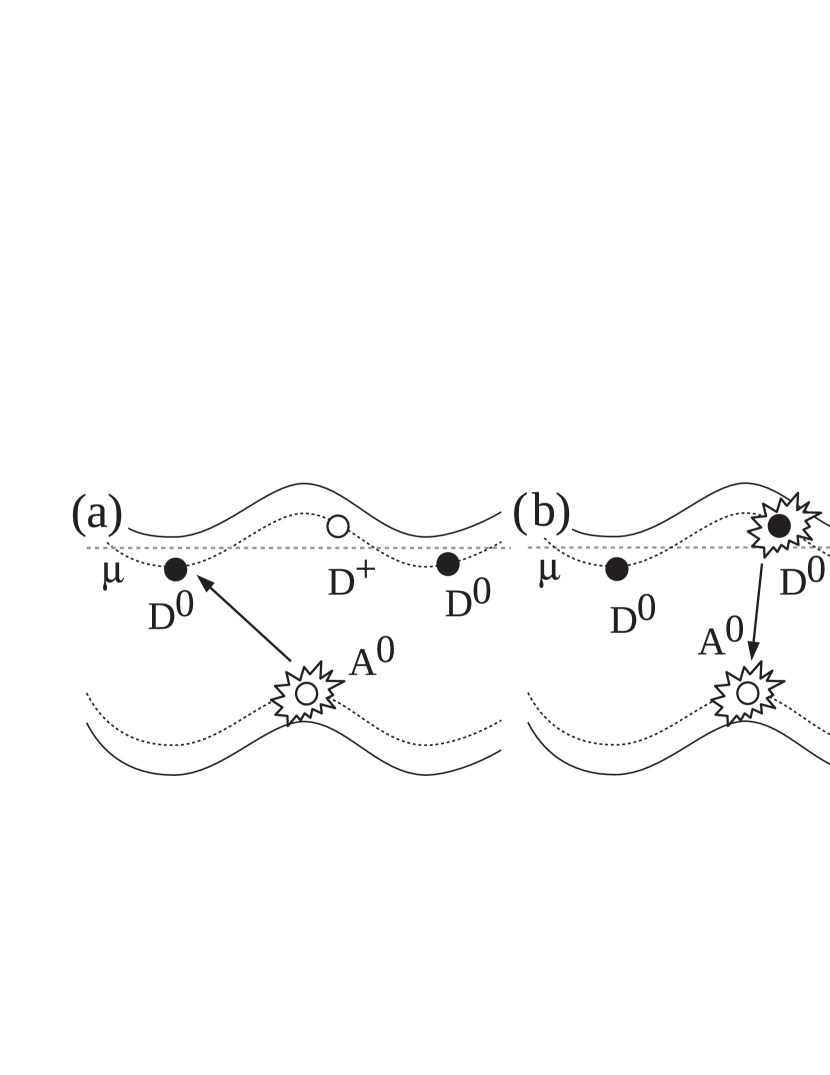
Figure 1: The energy band diagram under different conditions. Photo-excited impurities neutralized via the optical pumping are marked with sparkles. (a) The case of low pump intensities. Photo-excited, non-equilibrium donors and acceptors are rare and distant therefore photo-excited, non-equilibrium acceptors recombine with equilibrium donors. (b) The case of high pump intensities. Photo-excited, non-equilibrium donors and acceptors recombine with each other.

II Numerical simulation

We numerically simulate the energy distribution of donors and acceptors in compensated semiconductor at the temperature $T=0$ using the energy minimization algorithm via one-electron hopping Metropolis et al. (1953); Davies et al. (1984). Every random realization is a cubic volume with periodic boundary conditions containing randomly distributed donors and acceptors. For definiteness here we discuss the case of an n-type semiconductor. In our calculations a number of donors equals $n_{d}=10240$ due to a computer memory limitation. A number of acceptors is defined as $n_{a}=K\cdot n_{d}$ where $K$ is a compensation. In the paper we present results calculated using the optimal donor concentration $N_{d}a_{b}^{3}=0.01$ which is close to the metal-insulator transition. In the case of larger concentrations our approach is not applicable because we consider the insulator state. Numerical simulations for lower concentrations is an extremely time-consuming process due to an exponentially small overlap integral in equation (1). For every random realization we find the so-called pseudo-ground energy state using a procedure described by Shklovskii and Efros in the Chapter 14 of Efros and Shklovskii (1984). The procedure finds out a state with local minimum of energy performing a sequence of one-electron hops which decrease the total energy of the system. The obtained pseudo-ground state is not a global minimum and the total energy still can be decreased via multi-electron hopping. For trial we have considered a two-electron hopping in our calculation. However it significantly increased the calculation time and had no influence on spectra of DA recombination.

Initially all acceptors are charged negatively, $n_{a}$ donors are charged positively and $n_{d}-n_{a}$ donors are neutral. We find an occupied donor with maximum one-electron potential energy $\epsilon_{i}$ and an empty donor with minimum one. If the energy of the occupied state exceeds the energy of the empty one we transfer the electron and repeat this procedure for other electrons until it is possible. After every electron transfer we recalculate all one-electron potential energies $\epsilon_{i}$ for all impurities.

Then we consider one-electron hops which can minimize the total electrostatic energy of the DA system. The energy difference of a one-electron hop equals to

$$\Delta_{ij}=\epsilon_{j}-\epsilon_{i}-\frac{e^{2}}{\varepsilon r_{ij}}.$$

We find a pseudo-ground state completing all possible hops with negative $\Delta_{ij}$.

Next we numerically calculate spectra of DA recombination using a following algorithm. In order to simulate an optical pumping of DA system in the pseudo-ground state we neutralize a part of donors and acceptors and again recalculate all one-electron potential energies. In a strict sense, the part of neutralized impurities monotonically depends on pump intensity via kinetic parameters of a system. For simplicity’s sake we term the percentage of neutralized donors and acceptors as a pump intensity $I$. We numerically simulate an energy distribution of the DA transition probability by means of summation of all transitions between all occupied donors and acceptors using equation (1) and the following formula

$$\hbar\omega=E_{g}-E_{d}-E_{a}+\frac{e^{2}}{\varepsilon r_{ij}}+(\epsilon_{i}-\epsilon_{j}).$$

In order to obtain smooth spectrum curves we average data over about 100 thousands of random realizations. We program our simulation using CUDA parallel computing for the performance improving. We emphasize that our model has only three independent dimensionless parameters: a concentration $N_{d}\cdot a_{b}^{3}$, a compensation $K$ and a pump intensity $I$ which equals to the percentage of photo-excited acceptors.

Figure 2: (color online) DA luminescence spectra numerically simulated for different pump intensities. Concentration of donors $N_{d}a_{b}^{3}=0.01$, compensation $K=0.1$. Pump intensities $I$ are equal to 1 — 1.56%, 2 — 6.25%, 3 — 25%, 4 — 50%, 5 — 85%, 6 — 95% and 7 — 100%, $P_{0}=32\pi p_{0}N_{d}a_{b}^{3}/E_{d}$.

Results of the DA recombination spectra simulation depending on pump intensity are presented in figure 2. At low pump intensities the dominating component of spectra is due to recombination of photo-excited acceptors with equilibrium neutral donors. It is strongly broadened by an electric field of positively charged donors. This component is located in the low energy side of the spectrum because these transitions occur at longer distances. While the pump intensity increases the component of photo-excited carriers grows at the high energy side. An interplay of these components leads to a high energy shift of the spectrum maxima with increasing pump intensity. Random electric fields broaden the low energy tail. The high energy tail is due to recombination of closest DA pairs. The influence of random fields on the high energy part of spectra is weak and one can describe it as $\sim E^{-4}$ similarly to the equation (3). At high pump intensities the influence of random electric fields decreases due to photo-neutralization of charged impurities. A simple validation test of our algorithm is to simulate the case of 100% pump intensity. In this case all impurities are neutral, random electric fields are absent, and the result coincides with the equation (3) as shown in figure 2 with a dashed line.

As mentioned above this algorithm neglects the kinetic behavior of the DA system. In order to estimate the role of an energy relaxation we repeat the energy minimization procedure after the photo-excitation and before the spectra calculation. We considered separately a relaxation of only electrons or only holes. Results of these simulations will be discussed in section IV.

III Analytical calculation of luminescence spectra

In the limit of low compensation all ionized impurities form complexes due to Coulomb correlation (Chapter 3 of Efros and Shklovskii (1984)). Generally an acceptor forms a pair with the nearest donor. Such pairs are called 1-complexes with respect to the number of charged donors per one acceptor. Approximately 97.4% of acceptors form 1-complexes; however some acceptors form 0-complexes and in the vicinity of some acceptors there are two charged donors which form a 2-complex.

Here we considered the donor-acceptor luminescence of 1-complexes. At low pumping, an acceptor captures the photo-excited hole from the valence band and the nearest donor remains charged; therefore a hole recombines with the next neutral donor. Taking into account the influence of the charged donor on the transition energy, and neglecting the electric fields of others, more distant impurities, we can describe the shape of the spectral line of such transitions analytically. This component of DA recombination is a monomolecular process and we term this part as a three-center model.

At high pump intensities, the probability of simultaneous filling of donor and acceptor from one 1-complex increases. Because of the higher overlap of the wave functions, the recombination of such pairs dominates in the spectrum. The influence of electric fields on the transition energy in this case can be taken into account statistically, using the distribution of the electric field in a model of randomly located dipoles formed by ionized donors and acceptors. In this model, we assume that the electric field does not vary at a distance between the donor and the acceptor which is correct for the limit of small compensation.

In the analytical model we neglect the energy relaxation of charge carriers on impurities. In a certain approximation, this is equivalent to the high recombination rate when all trapped carriers recombine earlier than they are thermally activated back to the band.

We consider a random distribution of photo-excited carriers among DA pairs. It means that the probability to neutralize an impurity is proportional to $I$. Therefore the probability to obtain a neutral DA pair is proportional to $I^{2}$, while the probability to obtain a partly neutralized DA pair is proportional to $I(1-I)$. In order to compare spectra with different pump intensities we normalize results by $I$. It means that spectra in three-center model we multiply by $(1-I)$ while spectra in random dipoles model have $I$ coefficient.

III.0.1 The three-center model of the donor-acceptor recombination

At low pump intensities, we consider a three-center system presented in figure 3 which consists of two donors and one acceptor. Initially the three-center system consist of the ionized acceptor, the ionized donor which is the closest to the acceptor and the neutral equilibrium donor. Under the condition of weak optical pumping photo-excited holes and electrons are rare and DA pairs mostly capture only one type of carriers. Consequently, a recombination mainly occurs between the photo-excited neutral acceptor and the neutral equilibrium donor. In such a system, the closest to acceptor positively charged donor significantly changes the donor-acceptor recombination energy, which is equal to

$$E_{12}=\frac{e^{2}}{\varepsilon r_{1}}+\frac{e^{2}}{\varepsilon r_{2}}-\frac{e^{2}}{\varepsilon r_{12}}.$$

where

$$r_{12}=\sqrt{r_{1}^{2}+r_{2}^{2}-2r_{1}r_{2}\cos\theta}.$$

Figure 3: The three-center system consist of two donors and one acceptor. The donor nearest to the acceptor is ionized and another donor and the acceptor are neutral.

For the three-center system the probability of the photon emission with energy $E$ can be calculated as

$$P(E)=p_{0}(1-I)\int\limits_{0}^{+\infty}N_{d}4\pi r_{1}^{2}dr_{1}\int\limits_{0}^{r_{1}}N_{d}2\pi r_{2}^{2}dr_{2}\int\limits_{0}^{\pi}\sin\theta d\theta$$

$$\times\delta(E-E_{12})\exp\left(-\frac{2r_{1}}{a_{B}}\right)\exp\left(-\frac{4\pi}{3}r_{2}^{3}N_{d}\right)$$

The last factor in the integral describes the probability that the donor at the distance $r_{2}$ is the closest to the acceptor, and therefore this particular donor is ionized. In our calculations, this factor is always close to 1 because $r_{1}$ and $r_{2}$ are of the order of the donor radius $a_{B}\ll N_{d}^{-1/3}$.

We proceed from integration over the angle to integration over the transition energy

$$\frac{\partial E}{\partial\cos\theta}=-\frac{e^{2}r_{1}r_{2}}{\varepsilon\left(r_{1}^{2}+r_{2}^{2}-2r_{1}r_{2}\cos\theta\right)^{3/2}}$$

$$=-\left(\frac{\varepsilon}{e^{2}}\right)^{2}r_{1}r_{2}\left(\frac{e^{2}}{\varepsilon r_{1}}+\frac{e^{2}}{\varepsilon r_{2}}-E\right)^{3}$$

$$P(E)=p_{0}(1-I)\int\limits_{0}^{+\infty}N_{d}4\pi r_{1}^{2}dr_{1}\int\limits_{0}^{r_{1}}N_{d}2\pi r_{2}^{2}dr_{2}\int dE\frac{\partial\cos\theta}{\partial E}$$

$$\times\delta(E-E_{12})\exp\left(-\frac{2r_{1}}{a_{B}}\right)\exp\left(-\frac{4\pi}{3}r_{2}^{3}N_{d}\right)$$

The $\delta$ -function allows us to calculate the energy integral

$$P(E)=8\pi p_{0}(1-I)N_{d}^{2}\left(\frac{e^{2}}{\varepsilon}\right)^{2}$$

$$\times\int\limits_{0}^{+\infty}r_{1}\exp\left(-\frac{2r_{1}}{a_{B}}\right)dr_{1}\int\limits_{0}^{r_{1}}\frac{r_{2}\exp\left(-\frac{4\pi}{3}r_{2}^{3}N_{d}\right)}{\left(\frac{e^{2}}{\varepsilon r_{1}}+\frac{e^{2}}{\varepsilon r_{2}}-E\right)^{3}}dr_{2}$$ (4)

Since the further analytical integration is not possible, the calculations were performed numerically under the conditions

$$E\leq\frac{e^{2}}{\varepsilon r_{1}}+\frac{e^{2}}{\varepsilon r_{2}}-\frac{e^{2}}{\varepsilon\left(r_{1}+r_{2}\right)}$$

$$E\geq\frac{e^{2}}{\varepsilon r_{1}}+\frac{e^{2}}{\varepsilon r_{2}}-\frac{e^{2}}{\varepsilon\left(r_{1}-r_{2}\right)}$$

It is also necessary to exclude from consideration the three-center states in which both donors are charged and form the 2-complex. Such complexes form under the conditions

$$E-\frac{e^{2}}{\varepsilon r_{1}}>\mu$$

$$E-\frac{e^{2}}{\varepsilon r_{2}}>\mu.$$

Here $\mu$ is a chemical potential. In the limit of low compensation the chemical potential can be found analytically $\mu=0.99N_{d}^{1/3}e^{2}/\varepsilon$(Chapter 3 of Efros and Shklovskii (1984)). There is no analytical expression for chemical potential in the case of an intermediate compensation but it can be calculated numerically Efros et al. (1979).

Numerically simulated spectra of transitions between photo-excited acceptors and equilibrium neutral donors and luminescence spectra calculated in the three-center model are shown in figures 4 and 5 (curves 1 and 3, correspondingly). At low compensation (figure 4) our analytical calculations are in a good agreement with our simulation results. At high compensation (figure 5) a difference between two curves arises. The three-center model underestimates the broadening of the low-energy tail, however the qualitative similarity still persists.

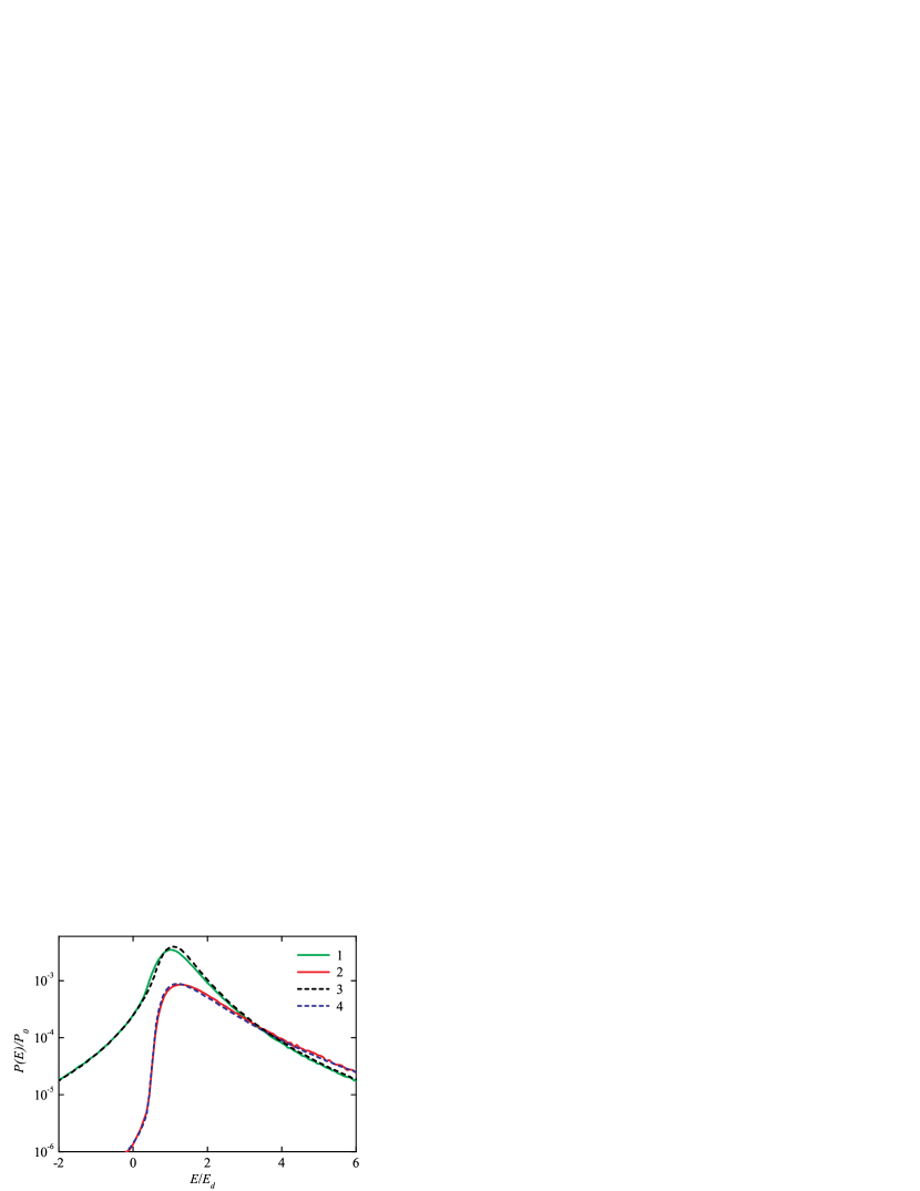
Figure 4: (color online) Luminescence spectra of equilibrium (curves 1 and 3) and photo-excited (curves 2 and 4) electrons. Dashed lines show spectra calculated analytically using equations (III.0.1) and (III.0.2). Solid lines are obtained by numerical simulations. Concentration of donors $N_{d}a_{b}^{3}=0.01$, compensation $K=0.025$, pumping $I=6.25\%$, $P_{0}=32\pi p_{0}N_{d}a_{b}^{3}/E_{d}$.

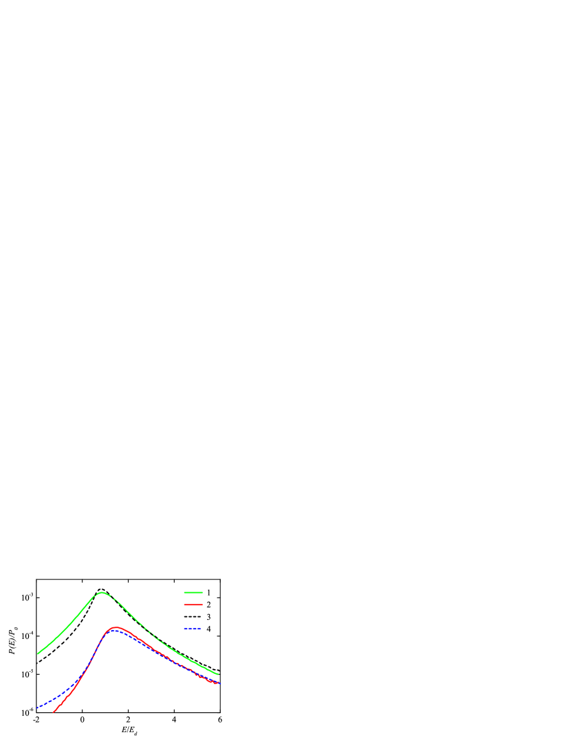
Figure 5: (color online) Luminescence spectra of equilibrium (curves 1 and 3) and photo-excited (curves 2 and 4) electrons. Dashed lines show spectra calculated analytically using equations (III.0.1) and (III.0.2). Solid lines are obtained by numerical simulations. Concentration of donors $N_{d}a_{b}^{3}=0.01$, compensation $K=0.5$, pumping $I=6.25\%$, $P_{0}=32\pi p_{0}N_{d}a_{b}^{3}/E_{d}$.

III.0.2 Random dipoles model

At high pumping, the main contribution to the luminescence spectrum is made by the recombination of photo-exited acceptors and donors from one 1-complex. The donor and acceptor within one pair are close to each other, so the transition probability is much higher than for the centers from different pairs. The main line broadening for closely located states is due to random electric fields in the material. The transition energy in an electric field $F$ can be written as

$$E=\frac{e^{2}}{\varepsilon r}+eFr\cos\theta$$

Here $\theta$ is the angle between the direction of the electric field and the line connecting the donor and the acceptor. This formula is valid if the electric field is constant on the scale of the recombination length, which is well satisfied only for low compensation. In the opposite case of the high compensation the recombination length is comparable with the mean distance between ionized impurities, therefore our approach is not applicable.

An electrically neutral system of randomly distributed point charges can be represented as a set of randomly oriented dipoles. Such an approach for dipoles with equal dipole moment modulus was first used by Holtsmark Holtsmark (1919) to describe electric fields in plasma. Shklovskii and co-authors considered a more general case when the magnitude of the dipole moment modulus is also random for the photoconductivity of compensated semiconductors Kogan et al. (1980). In this case the distribution function of a random electric field modulus $F$ is given by

$$f(F)=\frac{4}{\pi F_{md}}\frac{(F/F_{md})^{2}}{\left[1+(F/F_{md})^{2}\right]^{2}}$$

Here $F_{md}$ is the most probable electric field.

$$F_{md}=2.515\frac{KeN_{d}^{2/3}}{\varepsilon}$$

Then the probability of emission of a photon with an energy $E$ can be calculated as

$$P(E)=p_{0}I\int\limits_{0}^{+\infty}N_{d}2\pi r^{2}dr\exp\left(-\frac{2r}{a_{B}}-\frac{4\pi}{3}r^{3}N_{d}\right)$$

$$\times\int\limits_{0}^{\pi}\sin\theta d\theta\int\limits_{0}^{+\infty}dF\delta\left(E-\left(\frac{e^{2}}{\varepsilon r}+eFr\cos\theta\right)\right)f(F)$$

For further calculations we will make a change of the variable in the integral over the electric field to $T=F\cos\theta$. We will separately consider the integral over $\theta$ in which we will change the variable to $x=\cos\theta$ and denote $T/F_{md}=\alpha$

$$2\int\limits_{0}^{\pi/2}\sin\theta d\theta\frac{1}{\cos\theta}\frac{\left(\cfrac{T}{F_{md}\cos\theta}\right)^{2}}{\left[1+\left(\cfrac{T}{F_{md}\cos\theta}\right)^{2}\right]^{2}}=$$

$$=2\int\limits_{0}^{1}\frac{\left(\alpha/x\right)^{2}}{\left[1+\left(\alpha/x\right)^{2}\right]^{2}}\frac{dx}{x}=\frac{1}{1+\alpha^{2}}$$

Then the equation for the probability of transition can be rewritten as

$$P(E)=4p_{0}IN_{d}\int\limits_{0}^{+\infty}r^{2}dr\exp\left(-\frac{2r}{a_{B}}-\frac{4\pi}{3}r^{3}N_{d}\right)$$

$$\times\int\limits_{-\infty}^{+\infty}dT\delta\left(E-\left(\frac{e^{2}}{\varepsilon r}-eTr\right)\right)\cfrac{F_{md}}{F_{md}^{2}+T^{2}}$$

after integration over $T$, we obtain the final equation which was calculated numerically

$$P(E)={4p_{0}IN_{d}}\int\limits_{0}^{+\infty}rdr\exp\left(-\frac{2r}{a_{B}}-\frac{4\pi}{3}r^{3}N_{d}\right)$$

$$\times\cfrac{eF_{md}r^{2}}{e^{2}F_{md}^{2}r^{2}+\left(E-\cfrac{e^{2}}{\varepsilon r}\right)^{2}}$$ (5)

Let us note that in the limiting case of 100% pumping, all the impurity centers are neutral and do not produce random Coulomb fields. In this case $F_{md}\rightarrow~{}0$ and the fraction $\cfrac{1}{\pi}\cfrac{eF_{md}r}{e^{2}F_{md}^{2}r^{2}+\left(E-\cfrac{e^{2}}{\varepsilon r}\right)^{2}}$ converges to $\delta\left(E-\cfrac{e^{2}}{\varepsilon r}\right)$. In this case the resulting formula III.0.2 goes over into equation (3) which was obtained without taking into account random fields.

In figures 4 and 5 the numerically simulated spectra of transitions between photo-excited donors and acceptors are compared with the results of analytical calculation in the random dipoles model (curves 2 and 4, correspondingly). In the case of low compensation, a good agreement of the results is observed. There is a discrepancy between the analytical calculation and the simulation results at the low-energy tail at high compensation. Transitions with low energies correspond to recombination of very distant DA pairs. For such DA pairs a magnitude of the electric field is not constant over the size of the pair. As a result the random dipoles model for such low transition energies is not applicable because it overestimates the line broadening.

IV Discussion

Figures 4 and 5 show the DA recombination spectra for an n-type semiconductor with a donor concentration $N_{d}a_{b}^{3}=0.01$ and a pump intensity $I=6.25\%$ at different compensation levels, calculated both by numerical simulation and analytically. The relaxation of photo-excited carriers was not taken into account here.

In the numerical simulation of the photoluminescence spectrum, we separately calculated the luminescence of equilibrium and photo-excited donors. As was said in the theoretical part, the first case is well described by the three-center model, and the second one corresponds to random dipoles.

Such a two-component description allows us to explain a complicated behavior of DA recombination at different experimental conditions. Monomolecular and bimolecular components have different energy positions and its interplay leads to a high energy shift of DA line with increasing pump intensity. This energy shift is one of the known features of DA recombination and was observed experimentally Zacks and Halperin (1972). In the limit of high pump intensity the energy of the DA transition coincides with the energy of a free electron to acceptor recombination. In this case these two lines overlap and could be resolved only by different behavior in a magnetic field.

Monomolecular component dominates at low pump intensities and its electrostatic broadening does not depend on pump intensity. The broadening of a bimolecular component decreases with the pump intensity which is observed experimentally at high pump intensities Gershon et al. (2013).

In the case of a fast recombination rate when relaxation processes could be neglected two components of DA recombination are strongly overlapped and can not be spectrally resolved. However this situation can change if the energy relaxation rate is comparable with the recombination rate. We obtain the most demonstrative results of our numerical simulation in the case when minority photo-excited carriers relax before recombination while photo-excited majority carriers recombine without relaxation. This case is close to the experimental condition of p-type semiconductor because trapped electrons relax faster than holes. In figure 6 we present results of such simulation: two components of DA recombination are clearly resolved.

Two separate DA lines are often present in low temperature luminescence spectra of semiconductors Lahlou and Massé (1981); Rossi et al. (1970). A usual interpretation of this result involves a presence of two different kinds of impurity in a sample. However, our analysis shows that such two components, especially close ones, can originate from one kind of impurity.

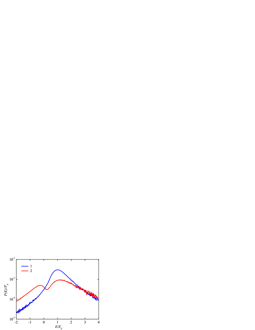
Figure 6: (color online) Luminescence spectra of DA recombination before (curve 1) and after (curve 2) full relaxation of photo-excited minority carriers Concentration of donors $N_{d}a_{b}^{3}=0.01$, compensation $K=0.1$, pumping $I=1\%$, $P_{0}=32\pi p_{0}N_{d}a_{b}^{3}/E_{d}$.

V Conclusion

The donor-acceptor luminescence spectra in compensated semiconductors were calculated numerically and analytically. The spectral and kinetic properties of luminescence at various pump intensities, concentrations, and compensations were studied. It was shown that the donor-acceptor recombination line consists of two components, the recombination of photo-excited holes with photo-excited electrons and the recombination of photo-excited holes with equilibrium electrons. These two components have different broadening mechanisms due to Coulomb correlations and random electric fields. The spectral form of both components in the low compensation limit have been obtained analytically. Numerical simulation results show that these simple analytical models not only agree with the numerical simulation at low compensation, but also qualitatively describe the spectra up to moderate compensations. Taking into account the possibility of photo-excited carriers relaxation we show that the two components can be resolved in the DA recombination spectra.