Textual Analogy Parsing: What’s Shared and
What’s Compared among Analogous Facts

Abstract

To understand a sentence like “whereas only 10% of White Americans live at or below the poverty line, 28% of African Americans do” it is important not only to identify individual facts, e.g., poverty rates of distinct demographic groups, but also the higher-order relations between them, e.g., the disparity between them. In this paper, we propose the task of Textual Analogy Parsing (TAP) to model this higher-order meaning. The output of TAP is a frame-style meaning representation which explicitly specifies what is shared (e.g., poverty rates) and what is compared (e.g., White Americans vs. African Americans, 10% vs. 28%) between its component facts. Such a meaning representation can enable new applications that rely on discourse understanding such as automated chart generation from quantitative text. We present a new dataset for TAP, baselines, and a model that successfully uses an ILP to enforce the structural constraints of the problem.

1 Introduction

The task of information extraction by and large seeks to populate a knowledge base with individuated facts extracted from text (Sarawagi, 2008). For example, given the sentence:

(E1) [According to the U.S. Census, whereas only 10% of White Americans live at or below the poverty line today]${}_{\textrm{C1}}$, [28% of African Americans do.]${}_{\textrm{C2}}$

one would extract two independent facts about voter registration, about the two distinct demographic groups. On the other hand, the theory of discourse maintains that part of the above sentence’s meaning inheres in the fact that clauses C1 and C2 are juxtaposed (Kehler, 2002). Thus the author intends that we consider them in relation to each other, inviting us to note, for example, a disparity of wealth distribution between demographic groups. To fail to capture this is to miss out on an important aspect of text understanding.

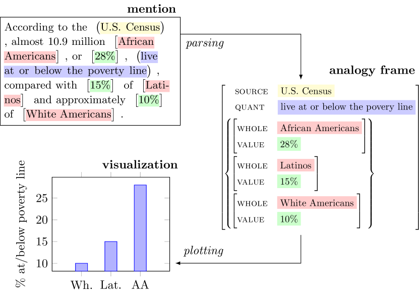
Figure 1: In textual analogy parsing (TAP), one maps analogous facts to semantic role representations and identifies analogical relations between them. Automated chart generation from text is a motivating application of TAP.

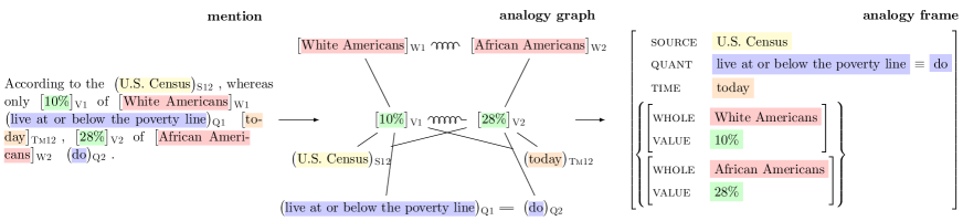
Figure 2: The mapping from utterance to TAP frame. Vertices in the graph are labeled with abbreviated semantic roles. Single lines represent edges between a value and other roles in its associated fact. Double lines represent coreference and synonymy. Springs represent analogy. Note that vertices connected by equivalence arcs, or any span which connects to both V1 and V2 via fact relations (i.e., scope), map to the shared content of the TAP frame. Analogous spans map to the compared content.

We propose the task of Textual Analogy Parsing (TAP) to explicitly capture such relational meaning between analogous facts in text. Concretely, TAP first maps a set of analogous facts to semantic role (SRL) representations, and then identifies the roles along which they are similar (the shared content) and along which they are distinct (the compared content)—see Figure 1. The resulting representation, the TAP frame, is a deeper representation than the one output by shallow discourse parsers (Taboada and Mann, 2006; Prasad et al., 2007; Pitler et al., 2009; Prasad et al., 2010; Surdeanu et al., 2015). Given (E1) above, a shallow discourse parser would classify the relation of contrast between C1 and C2—indicating that some salient differences exist in the meanings of the juxtaposed phrases—but without identifying the nature of those differences.

We focus on applying TAP to quantitative facts, because TAP frames can be used to create graphical plots from sentences with numbers, as in Figure 1. This new application could help to simplify complex quantitative text on the web Barrio et al. (2016); Leonhardt et al. (2017). We thus created an expert-annotated dataset of TAP frames over quantitative facts in the Wall Street Journal corpus (Marcus et al., 1999).

We model TAP by jointly predicting SRL representations of facts in a sentence, and higher-order semantic relations between them. Our main findings are that a neural architecture outperforms a log-linear baseline, well-chosen linguistic features help performance, and so does the use of an integer-linear programming (ILP) decoder that enforces the structural constraints of the task. Nevertheless, both quantitative and qualitative evaluation reveal room for improvement on TAP.

In sum, our main contributions are (1) a new task, Textual Analogy Parsing (TAP), that combines shallow semantic parsing with discourse meaning, (2) a dataset of TAP frames from quantitative newswire, and (3) a preliminary study of a new application, automated chart generation from text. All data and code, including standardized evaluation scripts, are made freely available.

2 A Semantic Representation of Analogy

Let us revisit the example sentence from the previous section (E1), where a pair of analogous quantitative facts about poverty rates of different demographic groups are presented in contrast. Individually, these can be represented using the semantic role structures in Figure 3, but representing them separately in this way fails to capture the fact that they are analogous, i.e., structurally and semantically similar but distinct.

Instead, we can explicitly show points of similarity and difference between them in the two-tiered frame structure in Figure 2, which we call a TAP frame. The outer tier of the TAP frame contains shared content, or information pertinent to all of the facts in question, and the inner tier contains compared content, the information that varies across the set of facts.

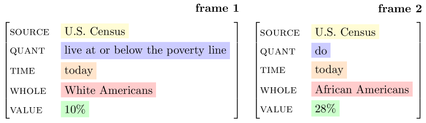
Figure 3: Two analogous quantitative facts represented independently, using the QSRL schema (Lamm et al., 2018).

Mapping from an utterance to a TAP frame requires three types of relational reasoning. Firstly, one must decompose the utterance into a set of facts, where a fact is represented as a set of semantic roles. Then, one must identify the shared content across facts by aligning roles that are semantically equivalent, in the sense that they are either the same span, are coreferent, or are synonymous. For example, in Figure 2 the phrase ‘U.S. Census’ occurs as the source of both facts because it scopes over the entire sentence in which they appear. Additionally, one must identify the compared content by aligning roles that are analogous, in the sense that they are semantically similar but nevertheless distinct. For example, the phrases ‘White Americans’ and ‘African Americans’ are analogous in our running sentence, playing the same role in their respective facts, while signifying distinct demographic groups.

(a)

$\big{[}$New England Electric$\big{]}$${}_{\textbf{\sc A1}}$ had $\big{[}$offered$\big{]}$${}_{\textbf{\sc Q1}}$ $\big{[}$$2 billion$\big{]}$${}_{\textbf{\sc V1}}$ to acquire $\big{(}$PS of New Hampshire$\big{)}$${}_{\textbf{\sc Th123}}$ , well below the $\big{[}$$2.29 billion$\big{]}$${}_{\textbf{\sc V2}}$ value $\big{[}$United Illuminating$\big{]}$${}_{\textbf{\sc A2}}$ places on its $\big{(}$bid$\big{)}$${}_{\textbf{\sc Q2}}$ and the $\big{[}$$2.25 billion$\big{]}$${}_{\textbf{\sc V3}}$ $\big{[}$Northeast$\big{]}$${}_{\textbf{\sc A3}}$ says its $\big{(}$bid$\big{)}$${}_{\textbf{\sc Q3}}$ is worth.

(b)

$\big{(}$First Boston$\big{)}$${}_{\textbf{\sc S12}}$ estimated that $\big{(}$UAL$\big{)}$${}_{\textbf{\sc Th12}}$ was $\big{(}$worth$\big{)}$${}_{\textbf{\sc Q12}}$ $\big{[}$$ 250 to $ 344 a share$\big{]}$${}_{\textbf{\sc V1}}$ based on $\big{[}$UAL’s results for the 12 months ending last June 30$\big{]}$${}_{\textbf{\sc C1}}$ , but only $\big{[}$$ 235 to $ 266$\big{]}$${}_{\textbf{\sc V2}}$ based on $\big{[}$a management estimate of results for 1989$\big{]}$${}_{\textbf{\sc C2}}$

Table 1: Representative sentences from the Quantitative TAP dataset. Co-indexing (e.g., A1/Q1) indicates when spans are part of the same QSRL fact. Parentheses indicate shared content spans and brackets indicate compared content spans. To parse (a), one must recognize that ‘to acquire PS of New Hampshire’ is elided but nevertheless an implied th(eme) in two of the clauses, and that ‘offered’ and ‘bid’ are contextually synonymous q(uantities). Moreover, one must note that the A(gents) are analogous, and hence part of the compared content. In (b), ‘First Boston’, ‘UAL’ and ‘worth’, contribute a s(ource), th(eme), and q(uantity) to the shared content respectively. Here, c(ause) roles are compared content.

3 The Quantitative TAP Dataset

Motivated by the application of automated graphical plot generation from text, we annotated a dataset of quantitative TAP frames from the Penn Treebank WSJ corpus (Marcus et al., 1999).

As our SRL representation of quantitative facts, we employ the Quantitative Semantic Role Labeling (QSRL) framework we previously defined in Lamm et al. (2018). Having identified a numerical value in text (e.g., 10%), QSRL asks, “what does this number measure?” to determine its associated quantity (e.g., a poverty rate). It might also identify, for example, the whole out of which this percentage is measured (e.g., the set of African Americans), and the time at which the quantity took on the value (e.g., today), etc. We employ all fifteen QSRL roles in our annotations.

	Train ($n=1000$)			Test ($n=100$)
	av.	max	tot.	av.	max	tot.
Count	1.4	3	1383	1.4	3	133
Length	2.6	16	–	2.6	7	–

Table 2: Dataset statistics (average per sentence, max per sentence, and total over the dataset) for the number of analogy frames (Count) and the number of values compared within each frame (Length).

Our annotations not only capture the relation between a quantitative predicate and its arguments, but also the higher-order analogy relations between them. The distinction is reflected in the sentences in Table 1 from the dataset: Colored spans are co-indexed when they participate in the same quantitative fact; spans with like roles surrounded by parentheses are shared content, meaning that they are either synonymous or co-referent; spans with like roles surrounded by brackets are compared content, meaning that they are analogous but semantically distinct.

To identify instances of quantitative analogy in the WSJ corpus, we first prune out any sentence having fewer than three numerical mentions, where a numerical mention is defined as a contiguous sequence of CD POS tags. Of those left, we manually identify those containing one or more quantitative analogies, i.e., ones in which numerical values are compared content. We estimate the incidence of these to be around 20%. A linguist then annotated 1,100 of these for analogy relationships. See Table 2 for a summary.

Using an independent set of expert annotations on 100 of these sentences, we measured a significant per-token label agreement of $0.882$ and edge label agreement of $0.991$ using Krippendorf’s $\alpha$.

Table 1 highlights some of the challenging linguistic phenomena in the data. With respect to identifying the shared content of a TAP frame, these can be coarsely divided into two sets. Firstly, in scope, ellipsis, and gapping, a single syntactic element serves as a role in multiple QSRL frames. This is exemplified by the phrase ‘PS of New Hampshire’ in Table 1(a): It is mentioned explicitly as a theme of the first fact, and only implied in the second two. Based on a random sample of 100 train sentences, we estimate that 86% of frames in the data exhibit these phenomena. Secondly, in synonymy and coreference, multiple elements appear in a sentence but contribute the same role to the shared content, e.g., ‘offered’ and ‘bid’ in Table 1(a). We estimate that 31% of frames in the data exhibit these phenomena.

One must learn to identify analogy relationships over a diverse set of compared content roles, with distinct semantic properties: in Table 1(a), agent is a compared content role, whereas in Table 1(b), cause is.

4 Modeling TAP in the Quantitative Setting

We model TAP by generating a typed analogy graph over spans of an input text that is isomorphic to the set of TAP frames in that text, e.g., Figure 2. Each vertex in the graph corresponds to a role-labeled span, and edges represent semantic relations between them.

In this graph, each fact is uniquely identified by a value vertex, which is connected via a fact edge to all of its associated roles. Any two shared content vertices across facts are connected by an equivalence edge, indicating that they are coreferent or synonymous. A single vertex can also be shared across facts by linking via a fact edge to more than one value vertex, suggesting a scopal relationship. Finally, any two vertices which are compared content in the graph are linked via an analogy edge.

More formally, given an utterance $\mathbf{x}$ with tokens $x_{1},\ldots,x_{n}$, let $G$ be a graph with vertices $V$ and edges $E$. For a vertex $v=(i,j,l)\in V$, $1\leq i<j\leq n$ are the start and end token indices of a span in $\mathbf{x}$ with role $l\in\mathcal{L_{Q}}\stackrel{{\scriptstyle\rm def}}{{=}}\{\textsc{value},\dots,\textsc{quant}\}$, the set of QSRL roles. For an edge $e=(v,v^{\prime},l)\in E$, $v,v^{\prime}\in V$ and $l\in\mathcal{L_{R}}\stackrel{{\scriptstyle\rm def}}{{=}}\{\textsc{fact},\textsc{equivalence},\textsc{analogy}\}$.

For $G$ so defined to encode a set of valid TAP frames, it must satisfy certain constraints:

1. Well-formedness constraints. For any two vertices $v,v^{\prime}\in V$, their associated spans must not overlap. Furthermore, every vertex must participate in at least one fact edge, i.e., no disconnected vertices.

2. Typing constraints. fact relations are always drawn from a value vertex to a non-value vertex. analogy and equivalence are only ever drawn between two vertices of the same role.

3. Unique facts. If a value vertex $v$ is connected to two distinct vertices $v^{\prime}$ and $v^{\prime\prime}$ of the same role via a fact edge, then $\textsc{equivalence}(v^{\prime},v^{\prime\prime})$ exists.

4. Transitivity constraints. analogy and equivalence edges are transitive: if $\textsc{equivalence}{}(v,v^{\prime})\in E$ and $\textsc{equivalence}(v^{\prime},v^{\prime\prime})\in E$ then $\textsc{equivalence}(v,v^{\prime\prime})\in E$ also. This also holds for analogy edges, but only when $v,v^{\prime}\mbox{ and }v^{\prime\prime}$ are value vertices.

1. Analogy. There must be at least one pair of analogous value vertices, and for each such pair, there must be a pair of analogous facts connected to them: if $v,v^{\prime}$ are two value vertices with $\textsc{analogy}(v,v^{\prime})\in E$, then there must also exist $w,w^{\prime}$ as two non-value vertices with $\textsc{fact}(v,w)\in E$, $\textsc{fact}(v^{\prime},w^{\prime})\in E$, $\textsc{analogy}(w,w^{\prime})\in E$.

Note that while these constraints rely on the choice of value as the role that grounds quantitative facts, they reflect the general idea that analogy is a structured mapping between meaning representations.

5 A Neural and ILP Model for TAP

We now present a neural and ILP model that predicts analogy graphs as defined in Section 4. Given a sentence, the neural model predicts a distribution over role-labeled spans with edges denoting semantic relations between them. Then, we use an ILP to decode while enforcing the TAP constraints defined in Section 4. Figure 4 presents an overview of the architecture.

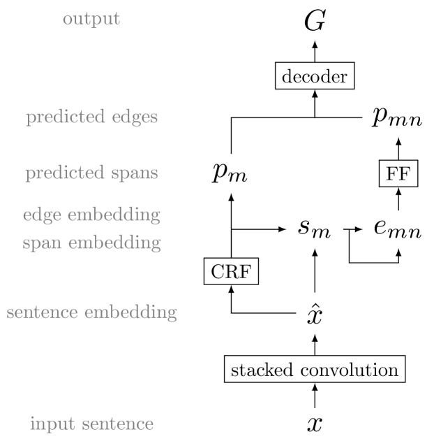
Figure 4: An overview of the proposed neural model: The sentence embedding represents features across the entire sentence using multiple convolutional layers. We then use a conditional random field (CRF) layer to predict labeled spans $p_{m}$ and to generate span and edge embeddings. We use a feedforward (FF) layer on the edge embeddings to predict edge labels $p_{mn}$. Together, $p_{m}$ and $p_{mn}$ form a distribution over edges and labels that we decode into TAP frames.

Context-sensitive word embeddings.

We first encode the words in a sentence by embedding each token using fixed word embeddings. We also concatenate a few linguistic features to the word embeddings, such as named entity tags and dependency relations. These features are generated using CoreNLP (Manning et al., 2014) and represented by randomly-initialized, learned embeddings for symbols together with the fixed word embedding of each token’s dependency head and the dependency path length between adjacent tokens. The token embeddings are then passed through several stacked convolutional layers Kim (2014). While the first convolutional layer can only capture local information, subsequent layers allow for longer-distance reasoning.

Span prediction.

Next, we feed the outputs of a single fully-connected hidden layer to a conditional random field (CRF) (Lafferty et al., 2001), which defines a joint distribution over per-token role labels. We thus obtain spans from this distribution corresponding to vertices of the graph described in Section 4 by merging contiguous role-labels in the maximum likelihood label sequence predicted by the CRF.

Edge prediction with PathMax features.

For edge prediction, we use the spans identified above to construct span and edge embeddings: for every span $(i,j)$ that was predicted, we construct a span vector $s_{m}=\sum_{k=i}^{j}\hat{x}_{k}$. We also construct a role-label score vector for the span, $p_{m}$ by summing the role-label probability vectors of its constituent tokens. Then, for every vertex pair $(m,n)$, we construct an edge representation $e_{mn}$. The basis of this representation is simply the concatenation of the span representations, the sum of the span representations, their respective role-label score vectors $p_{m}$ and $p_{n}$, and relative token distances.

To capture long-distance phenomena like scope, we also incorporate features into $e_{mn}$ from the dependency paths between the two spans by max-pooling the (learned) dependency relation embeddings along the path between the tokens. When computing the representation between two spans, we take the average of the path embedding between each pair of tokens within them. We call this extension PathMax.

The resulting edge representation $e_{mn}$ is passed through a single fully-connected hidden layer and an output layer to predict a distribution over edge labels $p_{mn}$, for each pair of spans.

Training.

The supervised data described in Section 3 provides gold spans and edges between them. Thus we define a loss function with two terms: one for the log-likelihood of the span labels output by the CRF model, and one for the cross-entropy loss on the edge labels. We train the span and edge components of the model jointly.

Decoding.

We consider two methods for decoding the span-level and edge-level label distributions $p_{m}$ and $p_{m,n}$ into a labeled graph respecting the constraints described in Section 4.

As a simple greedy method to enforce these constraints, we begin by picking the most likely role for each span and edge and then discarding any edges and spans that violate the well-formedness (1) and typing constraints (2). We then enforce transitivity constraints (4) by incrementally building a cluster of analogous and equivalent spans. We then resolve the unique facts constraint (3) by keeping only the span with highest fact edge score. Finally, for every cluster of analogous value spans, we check that the analogy constraint (5) holds and if not, discard the cluster.

We also implement an optimal decoder that encodes the TAP constraints as an ILP (Roth and Yih, 2004; Do et al., 2012). The ILP tries to find an optimal decoding according to the model, subject to hard constraints imposed on the solution space. For example, we require that solutions satisfy the ‘connected spans’ constraint:

$$\forall s\exists s^{\prime}:e(s,s^{\prime},\textsc{fact}{})$$

In plain English, this says that every span $s$ in a solution must be connected via a fact edge to some other span $s^{\prime}$. See the supplementary material for the full list of constraints we employ. We solve the ILPs with Gurobi Gurobi Optimization, Inc. (2018).

6 Experiments

We now describe the experimental setup of our neural model (Section 5) on the dataset of TAP frames we created (Section 3). Results and discussion are reported in Section 7.

Evaluation metrics.

The primary metric we use to measure the accuracy of a system on frame prediction is the precision, recall and $F_{1}$ between the labeled vertex-edge-vertex triples predicted by the model and those in the gold parse. If there are multiple predicted spans that overlap with a single gold span or vice versa, we find a matching of predicted and gold spans that maximizes overlap.

In addition to the primary metric, we also report precision, recall and $F_{1}$ when predicting labeled (non-value) spans and predicting labeled edges before performing any decoding. We also use the matching process described above for both these sets of metrics. Standardized evaluation code is provided with the dataset.

Experimental setup.

We compare the neural models presented in Section 5 in addition to a log-linear baseline. The log-linear baseline uses the same fixed word embeddings as the neural model in addition to the named entity and dependency parse features described in Section 5. The key difference is that instead of learning a sentence embedding or hidden layers, the log-linear model simply uses a CRF to predict span labels directly from fixed input features, and then uses a single sigmoid layer to predict edge labels from deterministic edge embeddings, $e_{mn}$.

For the neural models, we used three convolutional layers for sentence embedding with a filter size of 3. Every layer other than the input layer used a hidden dimension of 50 with ReLU nonlinearities. We introduced a single dropout layer ($p=0.5$) between every two layers in the network (including at the input). We used 50-dimensional GloVe embeddings (Pennington et al., 2014) learned from Wikipedia 2014 and Gigaword 5 as pre-trained word embeddings, and initialized the embeddings for the features randomly. We chose relatively low input- and hidden-vector dimension because of the size of our data. The network was trained for 15 epochs using ADADELTA (Zeiler, 2012) with a learning rate of $1.0$. All models were implemented in PyTorch (Paszke et al., 2017).

			Frame prediction
Model	Feats.	Dec.	P	R	$F_{1}$
Log-linear	$\checkmark$	gr.	46.3	21.8	29.7
Log-linear	$\checkmark$	opt.	37.1	27.5	31.6
Neural	$\times$	gr.	50.7	38.4	43.7
Neural	$\times$	opt.	52.8	48.6	50.6
Neural	$\checkmark$	gr.	54.9	57.4	56.1
Neural	$\checkmark$	opt.	56.4	68.8	62.0

Table 3: Performance of models on the test data. Combining the neural model with linguistic features and using an optimal decoder to enforce semantic constraints led to the best performance.

7 Results and Discussion

Frame prediction results on the test set are summarized in Table 3. Our three main findings are that (i) the neural network model far outperforms the log-linear model on our frame metric, (ii) including linguistic features further increases performance, and (iii) so does using an optimal decoder over a greedy method.

	Span prediction
Model	P	R	$F_{1}$
Log-linear (all feats.)	42.8	82.3	56.3
Neural (no feats.)	41.7	79.1	54.6
Neural (all feats.)	41.5	79.2	54.4
w/o NER	41.6	79.1	54.5
w/o dep.	41.2	77.5	53.8
w/o CRF	36.1	73.1	48.3

Table 4: Performance of models on labeled (non-value) span prediction during cross-validation prior to decoding. We found using a CRF to be the most important aspect: simply using fixed word vectors with a CRF (i.e., the log-linear model) was sufficient to predict spans.

	Edge prediction
Model	P	R	$F_{1}$
Log-linear (all feats.)	33.6	15.7	18.9
Neural (no feats.)	73.7	65.8	68.7
Neural (all feats.)	74.4	75.6	74.7
w/o NER	74.8	72.2	73.1
w/o dep.	73.4	65.0	68.2
w/o PathMax.	72.8	64.0	67.2

Table 5: Performance of models on labeled edge prediction during cross-validation prior to decoding. We found that both dependency label (dep.) and path features (PathMax) help significantly.

Quantitative error analysis.

To better understand which aspects of our model contribute to the task, we perform an ablation study on the span and edge predictions of our model prior to decoding.

With respect to span prediction (Table 4), we found that the fixed word vectors, along with a CRF, were able to capture the information needed to identify QSRL role-spans. Indeed, the log-linear baseline, which directly uses these word vectors as features for a CRF, did the best at span prediction. We believe that the drop in performance from introducing hidden layers with the neural models is a result of the model updating its span representations to do better edge prediction.

While the log-linear model did well at predicting spans, it did a poor job predicting edges, indicating that learning to extract higher-order features from learned span embeddings is necessary for identifying semantic relations between them (Table 5). We also found that linguistic features were important: in particular, we found that syntactic features – the dependency path features (PathMax) and dependency labels – played a big role in edge prediction, followed by type information from NER tags.

Qualitative error analysis.

Our model is tasked with jointly identifying QSRL parses of analogous facts in a sentence, and analogy and equivalence relations among them. As described in Section 4, these pieces interact in mutually constraining ways, and thus it is possible for local errors to have global effects on predicted frames.

In Figure 5, for example, the model correctly identifies the gold time spans as part of a TAP frame, but mistakenly predicts that they are linked by equivalence, and thus modify the same value span. In the gold parse, they are linked by analogy, and modify distinct value spans. As a result of this misclassification, the model leaves out an entire QSRL fact from the resulting parse.

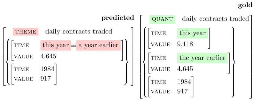
Figure 5: TAP frames for the sentence, ‘This year …daily contracts traded totaled 9,118, up from 4,645 a year earlier and from 917 in 1984.’ The model not only misclassifies the QSRL role of ‘daily contracts traded’, but also mistakenly identifies an equivalence between ‘this year’ and ‘the year earlier’. As a result, the value 9,118 is left without a compared content role, and is dropped.

In many cases, the model successfully identifies compared content roles between QSRL facts. In Figure 6, we show an example where it does not manage to do so. Here, unable to identify the analogy relation between the phrases ‘Those with a bullish view’ and ‘the dollar bears’, the model instead chooses two identical sequences ‘the dollar’ as the non-value compared content. Inspecting edge probability scores from the model before decoding reveals that the neural model thinks that the first instance of ‘the dollar’ in the sentence is semantically analogous to the second; it can be confused by surface similarity into classifying analogy relations.

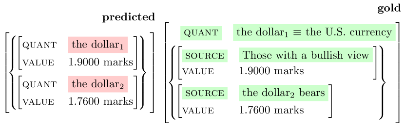
Figure 6: TAP frames for the sentence ‘Those with a bullish view see [the dollar]₁ trading up near 1.900 marks…while [the dollar]₂ bears see the U.S. currency trading around 1.7600 marks’. Among other errors, the model failed to identify analogous source spans and instead predicts that the two instances of the phrase ‘the dollar’ (indicated with indexing) in the sentence contribute non-value compared content.

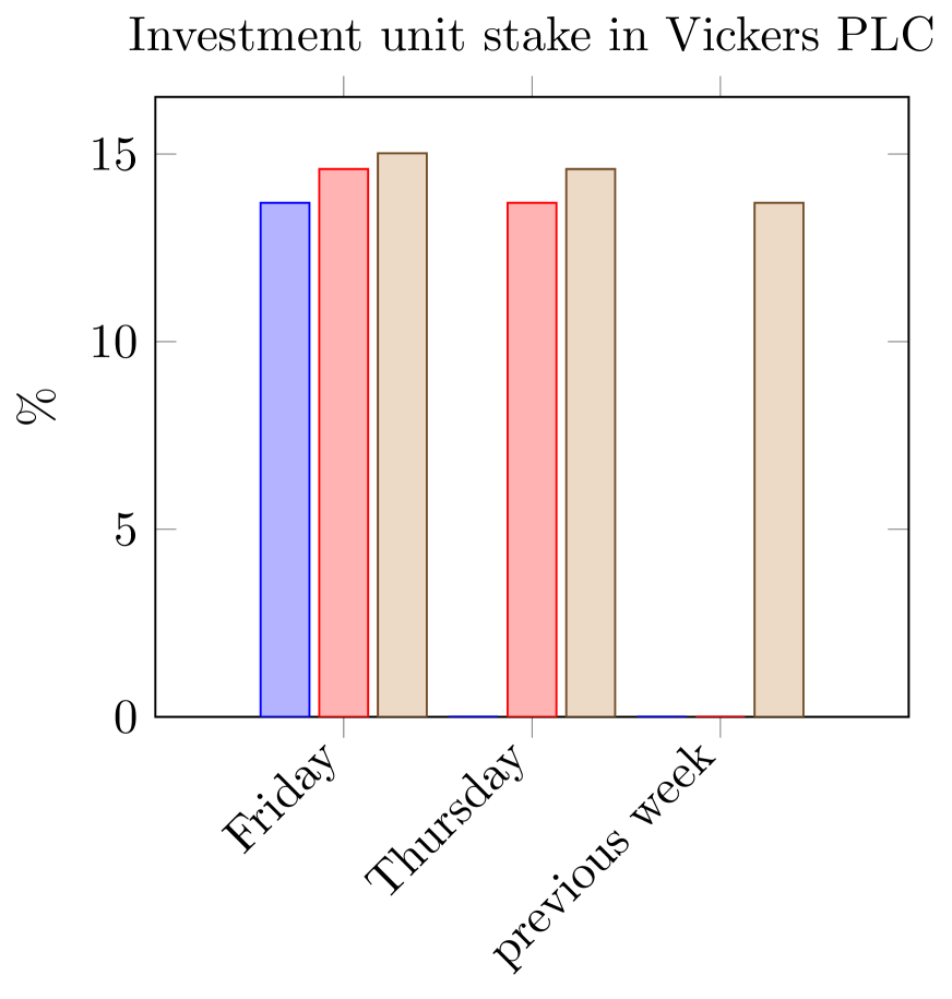
(a) Before constraints

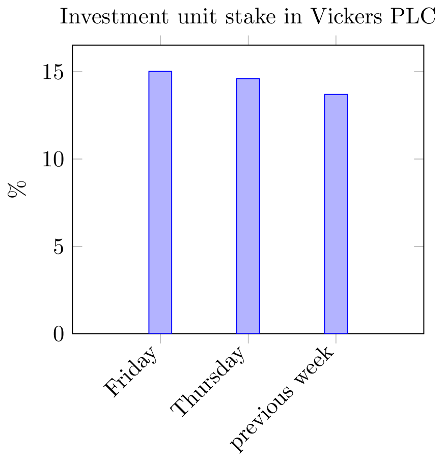
(b) After constraints

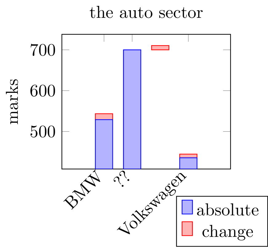
(c) Before constraints

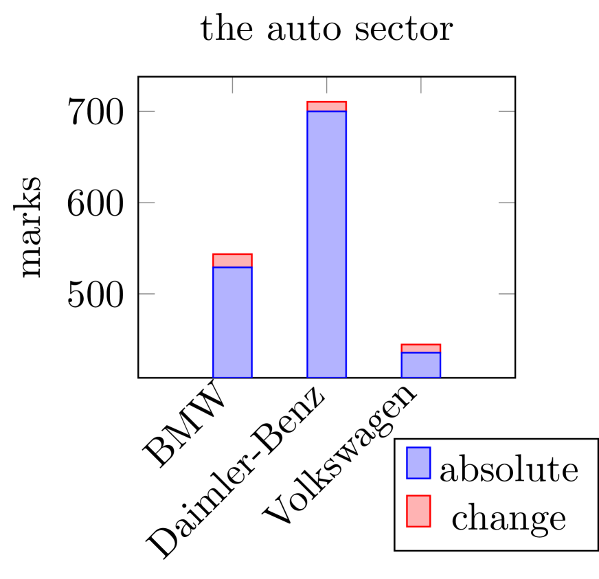
(d) After constraints

Figure 7: Charts generated from TAP frames. Charts (a) and (b) are generated from the sentence ‘Vicker’s PLC …raised its stake in the company Friday to 15.02% from about 14.6% Thursday and from 13.6% the previous week.’ Before imposing constraints, the neural model assigns multiple values to the time arguments ‘Thursday’ and ‘Friday’, over-extending their scope. Imposing structural constraints ensures the correct assignment of times to values. Charts (c) and (d) are generated from the sentence ‘In the auto sector, Bayerische Motoren Werke plunged 14.5 marks to 529 marks, Daimler-Benz dropped 10.5 to 700, and Volkswagen slumped 9 to 435.5.’ Here, the model fails to associate an absolute (blue) and relative (red) value pair with a theme role. The imposition of global constraints corrects this, linking them to the theme ‘Diamler-Benz’.

Application to plot generation.

As we have seen, textual analogy is frequently used to compare quantities along some axis of differentiation. For example, one might compare the stock prices of different companies, or describe the change in some quantity’s value over time. Such analogy relationships can alternately be expressed in the form of a plot.

Indeed, there is a natural correspondence between charts and TAP frames over quantitative facts: values of a quantitative TAP frame are plotted against other compared content roles, and elements of the shared content correspond with scopal chart elements, such as titles. This mapping is well-defined provided analogous values share units. We present some initial results exploring this direction.

In Figure 7, we deterministically plot TAP frames generated by our system both before and after the imposition of global analogy constraints, for two sentences in the data. In the first sentence, value spans are plotted against the time spans the model associates with their respective facts. In the second sentence, two analogy frames are plotted together, one reflecting the absolute values of the stock prices mentioned (blue) and the other reflecting the changes in prices mentioned (red). Units are extracted from value spans using simple pattern matching. Chart titles are only illustrative and were generated by stitching together shared content identified by our system.

Note that with the imposition of global constraints reflecting the structure of analogy, the system yields well-formed charts. Without these constraints, generated charts either have multiple y-axis values assigned to the same x-axis value, or have floating y-axis values with no grounding on the x-axis.

8 Related Work

Analogy.

In the cognitive science literature, analogy is a general form of relational reasoning unique to human cognition (Tversky and Gati, 1978; Holyoak and Thagard, 1996; Goldstone and Son, 2005; Penn et al., 2008; Holyoak, 2012). Our model of textual analogy is particularly influenced by Structure Mapping Theory (Falkenhainer et al., 1989; Gentner and Markman, 1997), an influential cognitive model of analogy as a structure-preserving map between concepts.

Within the NLP community, there has been much work focused on inferring lexical analogies between generic concepts, e.g., tennis:racket::baseball:bat (Mikolov et al., 2013; Turney, 2013), from global distributional statistics. Such analogies are generic, type-level patterns whose structure exists in the nature of the language; here, we are interested in specific analogies whose structure is conveyed by a particular sentence.

Discourse and Information Extraction.

TAP is an information extraction task that synthesizes ideas from semantic role labeling on the one hand and discourse parsing on the other. The former produces predicate-argument representations of individual facts in a text (Baker et al., 1998; Gildea and Jurafsky, 2002; Palmer et al., 2005); the latter identifies discourse relations between syntactic clauses (Taboada and Mann, 2006; Prasad et al., 2007; Pitler et al., 2009; Prasad et al., 2010; Surdeanu et al., 2015).

TAP first maps from syntax to a set of SRL-style representations, and then identifies structurally-constrained, higher-order relations among them. It is in this sense reminiscent of, but distinct from, work on causal processes by Berant et al. (2014).

Numbers in NLP.

There has been some work on understanding numbers in text. This includes quantitative reasoning (Kushman et al., 2014; Roy et al., 2015), numerical information extraction (Madaan et al., 2016), and techniques for making numbers more easily interpretable in text (Chaganty and Liang, 2016; Kim et al., 2016).

If pursued further, the application of plotting quantitative text that we discuss in this paper could help to clarify quantitative text on the web (Larkin and Simon, 1987; Barrio et al., 2016).

Neural modeling.

Recent work has shown the promise of sophisticated neural models on semantic role labeling (He et al., 2017). Similar to other such sequence prediction models, e.g., those for named entity recognition (Lample et al., 2016) or semantic role labeling (Zhou and Xu, 2015), our span prediction utilizes a neural CRF. Our model also has an edge-prediction component, which benefits from a simplified version of the PathLSTM model of Roth and Lapata (2016). Our edge-prediction model also uses an embedding concatenation component, which was inspired by recent work on neural coreference resolution Lee et al. (2017). He et al. (2017) also impose semantic constraints during prediction, but use A^∗ search instead of an ILP.

9 Conclusion

In this paper we have presented a new task, textual analogy parsing, or TAP. Given a sentence about a set of analogous facts, TAP outputs a frame representation that expresses the points of similarity and difference in their meanings.

We note that in the particular case of quantitative text, TAP frames correspond with charts. We develop a new dataset of TAP frames from quantitative newswire, and compare a variety models for TAP. Our best model employs a globally optimal decoder to enforce the structural constraints of analogy; its outputs can be mapped to well-formed charts of quantitative information extracted from text.

We view this work to be an exciting step in the direction of deeper discourse modeling. Future work might further extend the recovery of analogy as part of information extraction. This might include TAP outside of the quantitative domain, or TAP at the paragraph level.

Appendix A ILP constraints

The optimal decoder described in Section 5 implements the TAP constraints in Section 4 as an ILP. Here we present a representative set of our ILP constraints in the form of boolean expressions. In the following, variables $s$ refer to spans in an input text. $\mathcal{L_{Q}}=\{\textsc{quant}\dots\textsc{value}\}$ is the set of QSRL roles, and $\mathcal{L_{R}}=\{\textsc{equivalence}{},\textsc{analogy}{},\textsc{fact}{}\}$ is the set of semantic relations between them.

We let $r(s,l)=1$ if the decoder assigns to $s$ the role-label $l\in\mathcal{L_{Q}}$, and 0 otherwise, and let $\bar{r}(s)=1$ if for any role-label $l\in\mathcal{L_{Q}}$ $r(s,l)=1$, and zero otherwise. Similarly, we let $e(s,s^{\prime},l)=1$ if an edge is identified between spans $s,s^{\prime}$ with label $l\in\mathcal{L_{R}}$, and let $\bar{e}(s,s^{\prime})=1$ if for any edge label $l\in\mathcal{L_{R}}$, and 0 otherwise.

1. (Unique Roles) $\forall s:\sum_{l\in\mathcal{L_{Q}}}r(s,l)=\bar{r}(s)$

2. (Unique Edges) $\forall s,s^{\prime}:\sum_{l\in\mathcal{L_{R}}}e(s,s^{\prime},l)=\bar{e}(s,s^{\prime})$

3. (Connected Spans) $\forall s\exists s^{\prime}:e(s,s^{\prime},\textsc{fact}{})$

4. (Active Edges) $\forall s,s^{\prime}:\bar{e}(s,s^{\prime})\implies\bar{r}(s)\wedge\bar{r}(s^{\prime})$

5. (Equivalence and Analogy Typing) $\forall l,s,s^{\prime}$:

   • $e(s,s^{\prime},\textsc{equivalence}{})\implies\exists l:r(s,l)\wedge r(s^{\prime},l)$

   • $e(s,s^{\prime},\textsc{analogy}{})\implies\exists l:r(s,l)\wedge r(s^{\prime},l)$

6. (Fact Typing) $\forall s,s^{\prime}:e(s,s^{\prime},\textsc{fact}{})\implies(r(s,\textsc{value})\wedge\neg r(s^{\prime},\textsc{value}))\vee(r(s^{\prime},\textsc{value})\wedge\neg r(s,\textsc{value}))$

7. (Equality and Analogy Triangles) $\forall s,s^{\prime},s^{\prime\prime}:$

   • $e(s,s^{\prime},\textsc{equivalence}{})\wedge e(s^{\prime},s^{\prime\prime},\textsc{equivalence}{})\implies e(s,s^{\prime\prime},\textsc{equivalence}{})$

   • $e(s,s^{\prime},\textsc{analogy}{})\wedge e(s^{\prime},s^{\prime\prime},\textsc{analogy}{})\implies e(s,s^{\prime\prime},\textsc{analogy}{})$ but only when $r(s,\textsc{value})\wedge r(s^{\prime},\textsc{value})\wedge r(s^{\prime\prime},\textsc{value})$.

8. (Fact-Equality) $\forall l,s,s^{\prime},s^{\prime\prime}:$

   • $e(s,s^{\prime},\textsc{fact}{})\wedge e(s^{\prime},s^{\prime\prime},\textsc{equivalence}{})\implies e(s,s^{\prime\prime},\textsc{fact}{})$

   • $e(s,s^{\prime},\textsc{fact}{})\wedge e(s,s^{\prime\prime},\textsc{fact}{})\wedge r(s,l)\wedge r(s^{\prime},l)\implies e(s^{\prime},s^{\prime\prime})$

9. (Analogy Quadrangle) $\forall s,s^{\prime}:r(s,\textsc{value})\wedge r(s^{\prime},\textsc{value})\wedge e(s,s^{\prime},\textsc{analogy}{})\implies\exists s^{\prime\prime},s^{\prime\prime\prime}:e(s,s^{\prime\prime},\textsc{fact}{})\wedge e(s^{\prime},s^{\prime\prime\prime},\textsc{fact}{})\wedge e(s^{\prime\prime},s^{\prime\prime\prime},\textsc{analogy}{})$

References

- Baker et al. (1998) Collin F Baker, Charles J Fillmore, and John B Lowe. 1998. The Berkeley FrameNet Project. In Proceedings of the 17th International Conference on Computational Linguistics-Volume 1, pages 86–90.
- Barrio et al. (2016) Pablo J Barrio, Daniel G Goldstein, and Jake M Hofman. 2016. Improving Comprehension of Numbers in the News. In Proceedings of the 2016 CHI Conference on Human Factors in Computing Systems, pages 2729–2739.
- Berant et al. (2014) Jonathan Berant, Vivek Srikumar, Pei-Chun Chen, Abby Vander Linden, Brittany Harding, Brad Huang, Peter Clark, and Christopher D Manning. 2014. Modeling Biological Processes for Reading Comprehension. In Proceedings of the 2014 Conference on Empirical Methods in Natural Language Processing (EMNLP), pages 1499–1510.
- Chaganty and Liang (2016) Arun Chaganty and Percy Liang. 2016. How Much is 131 Million Dollars? Putting Numbers in Perspective with Compositional Descriptions. In ACL, pages 578–587.
- Do et al. (2012) Quang Xuan Do, Wei Lu, and Dan Roth. 2012. Joint Inference for Event Timeline Construction. In Proceedings of the 2012 Joint Conference on Empirical Methods in Natural Language Processing and Computational Natural Language Learning, pages 677–687.
- Falkenhainer et al. (1989) Brian Falkenhainer, Kenneth D Forbus, and Dedre Gentner. 1989. The Structure-Mapping Engine: Algorithm and Examples. Artificial Intelligence, 41(1):1–63.
- Gentner and Markman (1997) Dedre Gentner and Arthur B Markman. 1997. Structure Mapping in Analogy and Similarity. American Psychologist, 52(1):45.
- Gildea and Jurafsky (2002) Daniel Gildea and Daniel Jurafsky. 2002. Automatic Labeling of Semantic Roles. Computational linguistics, 28(3):245–288.
- Goldstone and Son (2005) Robert L Goldstone and Ji Y Son. 2005. The Transfer of Scientific Principles Using Concrete and Idealized Simulations. The Journal of the Learning Sciences, 14(1):69–110.
- Gurobi Optimization, Inc. (2018) Gurobi Optimization, Inc. 2018. Gurobi Optimizer Reference Manual. http://www.gurobi.com.
- He et al. (2017) Luheng He, Kenton Lee, Mike Lewis, and Luke Zettlemoyer. 2017. Deep Semantic Role Labeling: What Works and What’s Next. In Proceedings of the 55th Annual Meeting of the Association for Computational Linguistics (Volume 1: Long Papers), volume 1, pages 473–483.
- Holyoak and Thagard (1996) Keith Holyoak and Paul Thagard. 1996. Mental Leaps: Analogy in Creative Thought. MIT Press, Cambridge, Mass.
- Holyoak (2012) Keith J Holyoak. 2012. Analogy and Relational Reasoning. The Oxford Handbook of Thinking and Reasoning, pages 234–259.
- Kehler (2002) Andrew Kehler. 2002. Coherence, Reference, and the Theory of Grammar. CSLI Publications, Stanford, CA.
- Kim et al. (2016) Yea-Seul Kim, Jessica Hullman, and Maneesh Agrawala. 2016. Generating Personalized Spatial Analogies for Distances and Areas. In Proceedings of the 2016 CHI Conference on Human Factors in Computing Systems, pages 38–48.
- Kim (2014) Yoon Kim. 2014. Convolutional Neural Networks for Sentence Classification. In EMNLP.
- Kushman et al. (2014) Nate Kushman, Yoav Artzi, Luke Zettlemoyer, and Regina Barzilay. 2014. Learning to Automatically Solve Algebra Word Problems. In Proceedings of the 52nd Annual Meeting of the Association for Computational Linguistics (Volume 1: Long Papers), volume 1, pages 271–281.
- Lafferty et al. (2001) John D. Lafferty, Andrew McCallum, and Fernando C. N. Pereira. 2001. Conditional random fields: Probabilistic models for segmenting and labeling sequence data. In Proceedings of the Eighteenth International Conference on Machine Learning, ICML 2001, pages 282–289.
- Lamm et al. (2018) Matthew Lamm, Arun Chaganty, Dan Jurafsky, Christopher D. Manning, and Percy Liang. 2018. QSRL: A Semantic Role-Labeling Schema for Quantitative Text. In First Financial Narrative Processing Workshop at LREC 2018, Miyazaki, Japan.
- Lample et al. (2016) Guillaume Lample, Miguel Ballesteros, Sandeep Subramanian, Kazuya Kawakami, and Chris Dyer. 2016. Neural architectures for named entity recognition. In Proceedings of NAACL-HLT, pages 260–270.
- Larkin and Simon (1987) Jill H Larkin and Herbert A Simon. 1987. Why a Diagram is (Sometimes) Worth Ten Thousand Words. Cognitive science, 11(1):65–100.
- Lee et al. (2017) Kenton Lee, Luheng He, Mike Lewis, and Luke Zettlemoyer. 2017. End-to-end Neural Coreference Resolution. In Proceedings of the 2017 Conference on Empirical Methods in Natural Language Processing, pages 188–197.
- Leonhardt et al. (2017) David Leonhardt, Jodi Rudoren, Jon Galinsky, Karron Skog, Marc Lacey, Tom Giratikanon, and Tyson Evans. 2017. Journalism That Stands Apart: The Report of the 2020 Group. Technical report, The New York Times.
- Madaan et al. (2016) Aman Madaan, Ashish Mittal, G Ramakrishnan Mausam, Ganesh Ramakrishnan, and Sunita Sarawagi. 2016. Numerical Relation Extraction with Minimal Supervision. In AAAI, pages 2764–2771.
- Manning et al. (2014) Christopher D. Manning, Mihai Surdeanu, John Bauer, Jenny Finkel, Steven J. Bethard, and David McClosky. 2014. The Stanford CoreNLP Natural Language Processing Toolkit. In Association for Computational Linguistics (ACL) System Demonstrations, pages 55–60.
- Marcus et al. (1999) Michell P. Marcus, Beatrice Santorini, Mary Ann Marcinkiewicz, and Ann Taylor. 1999. Treebank-3 ldc99t42.
- Mikolov et al. (2013) Tomas Mikolov, Wen-tau Yih, and Geoffrey Zweig. 2013. Linguistic Regularities in Continuous Space Word Representations. In Proceedings of the 2013 Conference of the North American Chapter of the Association for Computational Linguistics: Human Language Technologies, pages 746–751.
- Morris (2014) Monique W. Morris. 2014. Black Stats. The New Press, New York, NY.
- Palmer et al. (2005) Martha Palmer, Daniel Gildea, and Paul Kingsbury. 2005. The Proposition Bank: An Annotated Corpus of Semantic Roles. Computational linguistics, 31(1):71–106.
- Paszke et al. (2017) Adam Paszke, Sam Gross, Soumith Chintala, Gregory Chanan, Edward Yang, Zachary DeVito, Zeming Lin, Alban Desmaison, Luca Antiga, and Adam Lerer. 2017. Automatic differentiation in PyTorch. In NIPS Workshop on Autodifferentiation.
- Penn et al. (2008) Derek C Penn, Keith J Holyoak, and Daniel J Povinelli. 2008. Darwin’s mistake: Explaining the discontinuity between human and nonhuman minds. Behavioral and Brain Sciences, 31(2):109–130.
- Pennington et al. (2014) Jeffrey Pennington, Richard Socher, and Christopher D. Manning. 2014. GloVe: Global Vectors for Word Representation. In Empirical Methods in Natural Language Processing (EMNLP), pages 1532–1543.
- Pitler et al. (2009) Emily Pitler, Annie Louis, and Ani Nenkova. 2009. Automatic sense prediction for implicit discourse relations in text. In Proceedings of the Joint Conference of the 47th Annual Meeting of the ACL and the 4th International Joint Conference on Natural Language Processing of the AFNLP, volume 2, pages 683–691.
- Prasad et al. (2010) Rashmi Prasad, Aravind K Joshi, and Bonnie L Webber. 2010. Exploiting Scope for Shallow Discourse Parsing. In LREC.
- Prasad et al. (2007) Rashmi Prasad, Eleni Miltsakaki, Nikhil Dinesh, Alan Lee, Aravind Joshi, Livio Robaldo, and Bonnie L Webber. 2007. The Penn Discourse Treebank 2.0 Annotation Manual. Technical report, Institute for Research in Cognitive Sciences.
- Roth and Yih (2004) Dan Roth and Wen-tau Yih. 2004. A Linear Programming Formulation for Global Inference in Natural Language Tasks. Technical report, Illinois University at Urbana-Champaign, Dept of Computer Science.
- Roth and Lapata (2016) Michael Roth and Mirella Lapata. 2016. Neural Semantic Role Labeling with Dependency Path Embeddings. In Proceedings of the 54th Annual Meeting of the Association for Computational Linguistics (Volume 1: Long Papers), volume 1, pages 1192–1202.
- Roy et al. (2015) Subhro Roy, Tim Vieira, and Dan Roth. 2015. Reasoning about quantities in natural language. Transactions of the Association for Computational Linguistics, 3:1–13.
- Sarawagi (2008) Sunita Sarawagi. 2008. Information Extraction. Foundations and Trends in Databases, 1(3):261–377.
- Surdeanu et al. (2015) Mihai Surdeanu, Tom Hicks, and Marco Antonio Valenzuela-Escarcega. 2015. Two Rractical Rhetorical Structure Theory Parsers. In HLT-NAACL, pages 1–5.
- Taboada and Mann (2006) Maite Taboada and William C Mann. 2006. Rhetorical Structure Theory: Looking back and moving ahead. Discourse Studies, 8(3):423–459.
- Turney (2013) Peter D Turney. 2013. Distributional semantics beyond words: Supervised learning of analogy and paraphrase. arXiv preprint arXiv:1310.5042.
- Tversky and Gati (1978) Amos Tversky and Itamar Gati. 1978. Studies of Similarity. Cognition and Categorization, 1(1978):79–98.
- Zeiler (2012) Matthew D Zeiler. 2012. ADADELTA: an adaptive learning rate method. arXiv preprint arXiv:1212.5701.
- Zhou and Xu (2015) Jie Zhou and Wei Xu. 2015. End-to-end Learning of Semantic Role Labeling Using Recurrent Neural Networks. In Proceedings of the 53rd Annual Meeting of the Association for Computational Linguistics and the 7th International Joint Conference on Natural Language Processing, volume 1, pages 1127–1137.