Contractible open manifolds which embed in no compact, locally connected and locally 1-connected metric space

Abstract.

This paper pays a visit to a famous contractible open 3-manifold $W^{3}$ proposed by R. H. Bing in 1950’s. By the finiteness theorem [Hak68], Haken proved that $W^{3}$ can embed in no compact 3-manifold. However, until now, the question about whether $W^{3}$ can embed in a more general compact space such as a compact, locally connected and locally 1-connected metric 3-space was unknown. Using the techniques developed in Sternfeld’s 1977 PhD thesis [Ste77], we answer the above question in negative. Furthermore, it is shown that $W^{3}$ can be utilized to produce counterexamples for every contractible open $n$-manifold ($n\geq 4$) embeds in a compact, locally connected and locally 1-connected metric $n$-space.

1. Introduction

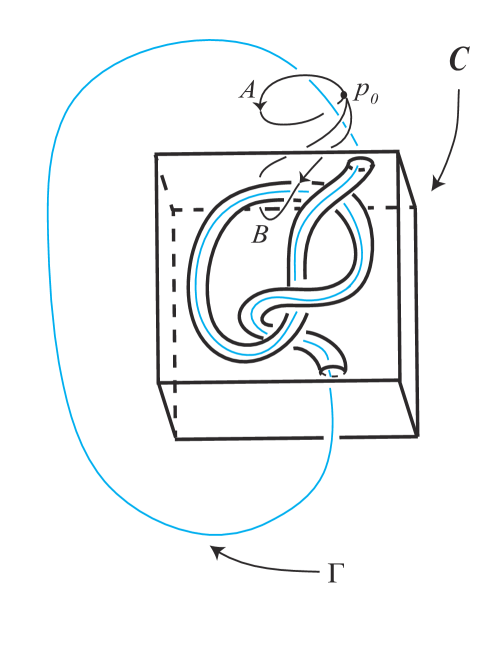
Counterexamples for every open 3-manifold embeds in a compact 3-manifold have been discovered for over 60 years. Indeed, there are plenty of such examples even for open manifolds which are algebraically very simple (e.g., contractible). A rudimentary version of such examples can be traced back to [Whi35] (the first stage of the construction is depicted in Figure 9) where Whitehead surprisingly found the first example of a contractible open 3-manifold different from $\mathbb{R}^{3}$. However, the Whitehead manifold does embed in $S^{3}$. In 1962, Kister and McMillan noticed the first counterexample in [KM62] where they proved that an example proposed by Bing (see Figure 1) doesn’t embed in $S^{3}$ although every compact subset of it does. In the meantime, they conjectured that Bing’s example is a desired counterexample, i.e., such example embeds in no compact 3-manifold. This conjecture was confirmed later by Haken using his famous finiteness theorem [Hak68] stating that there is an upper bound on the number of incompressible nonparallel surfaces in a compact 3-manifold. Similar examples can readily derive from Haken’s finiteness theorem (or see [MW79, Thm. 2.3]). In 1977, an interesting example (see Figure 10) was given in Sternfeld’s PhD dissertation [Ste77]. Instead of using Haken’s finiteness theorem, Sternfeld applied covering space theory to produce a contractible open $n$-manifold ($n\geq 3$) that embeds in no compact $n$-manifold. His constructions can be viewed as a modification of Bing’s, but he claimed that his examples cannot embed as an open subset in any compact, locally connected and locally 1-connected metric space, which is much more general than a compact manifold. More importantly, at the time of writing, Sternfeld’s constructions are the only known examples of such phenomenon in high dimensions.

Remark 1.

There is an error in Sternfeld’s dissertation which directly affects his whole argument. In the process of proving our main theorem, we correct this error, thereby, confirming the validity of his example (see Remark 2 in §4 for details).

It is natural to ask if Bing’s example can embed in a more general compact space, say, a compact absolute neighborhood retract or compact, locally connected and locally 1-connected 3-dimensional metric space. Here we answer the above question in negative.

Theorem 1.1.

$W^{3}$ embeds as an open subset in no compact, locally connected, locally 1-connected metric space. In particular, $W^{3}$ embeds in no compact $3$-manifold.

Making use of the high-dimensional construction developed in [Ste77], we extend Theorem 1.1 to all finite dimensions.

Theorem 1.2.

There exists a contractible open $n$-manifold $W^{n}$ ($n\geq 4$) which embeds as an open subset in no compact, locally connected, locally 1-connected metric $n$-space. Hence, $W^{n}$ embeds in no compact $n$-manifold.

The strategy of our proof heavily relies on the techniques and results from Sternfeld’s dissertation [Ste77]. Succinctly speaking, the key is to show that the union of $W^{3}$ and a 3-ball (advertised as a knot complement $K_{j}$) has a finite cover which contains infinitely many pairwise disjoint incompressible surfaces. Many results from [Ste77] will not be re-proved here, but we will take shortcuts afforded by knot theory and software GAP [GAP18] in this work.

The outline of this paper is: §2 gives a detailed review of the construction of Bing’s example and discusses its cruical connection with a knot space $K_{j}$. That is, showing Bing’s example can embed in no compact, locally connected and locally 1-connected metric space is equivalent to showing $\pi_{1}(K_{j})$ is not finitely generated. Towards that goal, in §3 we find the Wirtinger presentation of $\pi_{1}(K_{j})$ and in §4, we define an important surjection of $\pi_{1}(K_{j})$ onto $\mathbb{A}_{5}$. Meanwhile, we fix an error in Sternfeld’s dissertation. §5 paves the road for §6 by showing that the key ingredient is to focus on an object called a cube with a trefoil-knotted hole. §6 proves Theorem 1.1 by using results obtained from §2-§5. The proof of Theorem 1.2 is presented at the end of this section. In §7, we discuss some related questions of this work.

2. The construction of a 3-dimensional example

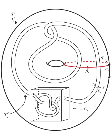
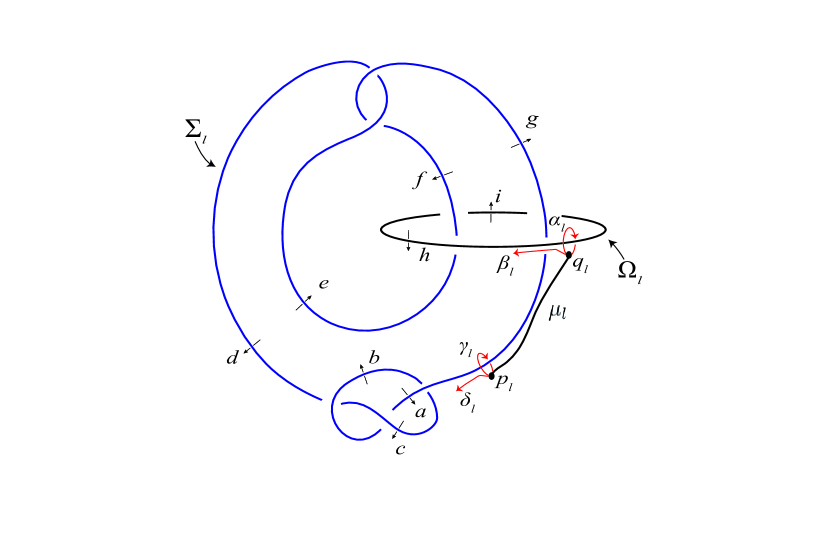
First, we reproduce the example originially proposed by Bing, i.e., a 3-dimensonal contractible open manifold $W^{3}$. Let $\{T_{l}|l=0,1,2,\dots\}$ be a collection of disjoint solid tori standardly embedded in $S^{3}$. Let the solid torus $T_{l}^{\prime}$ be embedded in $\operatorname{Int}T_{l}$ as in Figure 1. Let the oriented simple closed curve $\alpha_{l}$, $\beta_{l}$, $\gamma_{l}$ and $\delta_{l}$ be as shown in Figure 1. The curves $\alpha_{l}$ and $\beta_{l}$ are transverse in $\partial T_{l}$, and meet at the point $q_{l}\in\partial T_{l}$. In a similar fashion, the curves $\gamma_{l}$ and $\delta_{l}$ are transverse in $\partial T_{l}^{\prime}$, and meet at the point $p_{l}\in\partial T_{l}^{\prime}$. For $l\geq 1$, let $L_{l}=T_{l}\backslash\operatorname{Int}T_{l}^{\prime}$. Define an embedding $h_{l+1}^{l}:T_{l}\to T_{l+1}$ so that $T_{l}$ is carried onto $T_{l+1}^{\prime}$ with $h_{l+1}^{l}(\alpha_{l})=\delta_{l+1}$ and $h_{l+1}^{l}(\beta_{l})=\gamma_{l+1}$. $W^{3}$ is the direct limit of the $T_{l}$’s and denoted as $W^{3}=\lim\limits_{l\to\infty}(T_{l},h_{l+1}^{l})$. That is equivalent to view $W^{3}$ as the quotient space: $\sqcup_{l}T_{l}\xrightarrow{q}W^{3}$, where $\sqcup_{l}T_{l}$ is the disjoint union of the $T_{l}$’s and $q$ is the quotient map induced by the relation $\sim$ on $\sqcup_{l}T_{l}$. If $x\in T_{i}$ and $y\in T_{j}$, then $x\sim y$ iff there exists a $k$ larger than $i$ and $j$ such that $h_{k}^{i}(x)=h_{k}^{j}(y)$, where $h_{t}^{s}=h_{t}^{t-1}\circ h_{t-1}^{t-2}\circ\cdots\circ h_{s+2}^{s+1}\circ h_{s+1}^{s}$ for $t>s$. Let $\iota_{l}:T_{l}\hookrightarrow\sqcup_{l}T_{l}$ be the obvious inclusion map. The composition $q\circ\iota_{l}$ embeds $T_{l}$ in $W^{3}$ as a closed subset. The injectivity follows from the injectivity of $h_{k+1}^{k}$. It is closed since for $j>l$ the set $h_{j}^{l}(T_{l})$ is closed in $T_{j}$. Let $T_{l}^{*}$ denote $q\circ\iota_{l}(T_{l})$. $T_{l}^{*}$ is embedded in $T_{l+1}^{*}$ just as the way $h_{l+1}^{l}(T_{l})$ ($=T_{l+1}^{\prime}$) is embedded in $T_{l+1}$. Hence, Figure 1 can be viewed as a picture of the embedding of $T_{l}^{*}$ in $T_{l+1}^{*}$. In general, for $k>l$, $T_{l}^{*}$ is embedded in $T_{k}^{*}$ just as $h_{k}^{l}(T_{l})$ is embedded in $T_{k}$.

Figure 1. $L_{l}=T_{l}\backslash T_{l}^{\prime}$. The “inner” boundary component of $L_{l}$ is $\partial T_{l}^{\prime}$. The “outer” boundary component of $L_{l}$ is $\partial T_{l}$

Proposition 2.1.

$W^{3}$ is an contractible open connected $3$-manifold.

Proof.

By the construction described above, $W^{3}$ is an expanding union of $T_{l}^{*}$’s, hence, connected. The interior of each $h_{j}^{l}(T_{l})$ is open in $T_{j}$, so $\operatorname{Int}T_{l}^{*}$ is open in $W^{3}$. Since $T_{l}^{*}$ is contained in $\operatorname{Int}T_{l+1}^{*}$, $W^{3}$ is an open 3-manifold.

To show the contractibility of $W^{3}$, we first triangulate $W^{3}$ by choosing for each $T_{l}$ ($l\geq 0$), a simplicial subdivision such that each embedding $h_{k+1}^{k}$ ($k\geq 0$) is simplicial with respect to the chosen subdivision of its domain and range. Let $H:W^{3}\times[0,1]\to W^{3}$ be the contraction to be constructed. Define $H$ inductively on the skeleton of $W^{3}\times[0,1]$. Pick $p\in W^{3}$ to be the point to which we want to contract. Map each vertex cross $[0,1]$ to a path beginning at the vertex and ending at $p$. Let $\Delta^{(1)}$ be a 1-simplex of $W^{3}$. Define the restrictions $H|_{\Delta^{(1)}\times\{0\}}$ to be the identity and $H|_{\Delta^{(1)}\times\{1\}}$ to be the constant map taking all points to $p$. Note that $\partial\Delta^{(1)}$ lies in the 0-skeleta of $W^{3}$. $H$ has already been defined on $\partial\Delta^{(1)}\times[0,1]=\partial(\Delta^{(1)}\times[0,1])$. Note that $T_{l}^{*}$ contracts in $T_{l+1}^{*}$ (see Figure 1). $H$ can be extended to the rest of $\Delta^{(1)}\times[0,1]$ by the fact that $H|_{\partial(\Delta^{(1)}\times[0,1])}$ contracts in $W$. Doing this for all 1-simplexes so $H$ is well-defined on the 1-skeleta cross $[0,1]$. One can do this for 2- and 3-skeleta cross $[0,1]$ inductively. ∎

Definition 2.1.

A topological space $X$ is locally 1-connected at the point $x\in X$ if for each neighborhood $U$ of $x$ there is a neighborhood $V$ of $x$, $V\subset U$, such that every loop in $V$ contracts in $U$. We say that $X$ is locally 1-connected if $X$ is locally 1-connected at each of its points.

The approach of proving Theorem 1.1 does not rely on Haken’s finiteness theorem [Hak68]. Instead, we take advantage of the covering space argument in [Ste77].

Suppose there is a compact, locally connected, locally 1-connected metric space $U$ such that $U$ contains $W^{3}$ as an open subset. By taking the component of $U$ containing $W^{3}$ we may assume that $U$ is connected. Then the following result assures that $\pi_{1}(U\backslash\operatorname{Int}T^{*}_{0})$ must be finitely generated.

Lemma 2.2.

[Ste77, Lemma 1.1, P.7] If $X$ is a compact, connected, locally connected, locally $1$-connected metric space, then $\pi_{1}(X)$ is finitely generated.

Instead of working on $\pi_{1}(U\backslash\operatorname{Int}T^{*}_{0})$ directly, it is easier to focus on a knot space $K_{j}=S^{3}\backslash\operatorname{Int}h_{j}^{0}(T_{0})$ ($j\geq 1$). Combining with Claim 2, we have an observation as follows.

Claim 1.

$\pi_{1}(K_{j})$ is a homomorphic image of $\pi_{1}(U\backslash\operatorname{Int}T^{*}_{0})$.

Proof.

Let $p_{j}$ and $p_{j}^{\prime}$ be quotient maps in the commutative diagram (see Figure 2).

Figure 2. Commutative diagram

The inclusion, $\iota_{j}$, followed by $p_{j}$ induces the map $g_{j}$ since the restriction of $p_{j}$ on $T_{j}^{*}\backslash\operatorname{Int}T_{0}^{*}$ is to collapse $\partial T_{j}^{*}$ to a point. It’s not hard to see that $g_{j}$ is actually a homeomorphism. Since $\partial T_{j}^{*}$ is collared in $T_{j}^{*}\backslash\operatorname{Int}T_{0}^{*}$, Lemma 5.4 implies that $p_{j}^{\prime}$ induces a surjection on fundamental groups. By the commutativity of the diagram 2, $p_{j^{*}}^{\prime}=g_{j^{*}}^{-1}p_{j^{*}}\iota_{j^{*}}$, where $p_{j^{*}}^{\prime}$, $g_{j^{*}}$, $p_{j^{*}}$ and $\iota_{j^{*}}$ are the homomorphisms induced by maps $p_{j}^{\prime}$, $g_{j}$, $p_{j}$ and $\iota_{j}$ respectively. Since $p_{j^{*}}^{\prime}$ is a surjection, $g_{j^{*}}^{-1}p_{j^{*}}$ is also a surjection. Hence, $\pi_{1}((T_{j}\backslash\operatorname{Int}T_{0}^{*})/\partial T_{j}^{*})$ is a homomorphic image of $\pi_{1}(U\backslash\operatorname{Int}T_{0}^{*})$. According to the construction of $W^{3}$, the pair $(T_{j}^{*},T_{0}^{*})$ is homeomorphic to the pair $(T_{j},h_{j}^{0}(T_{0}))$. Then the claim follows from Claim 2. ∎

Since the rank of a group must be a least as large as that of any homomorphic image, it suffices to show that the rank of $\pi_{1}(K_{j})$ is unbounded.

The space $K_{j}$ is advertised as “knot space” is because it can be viewed as a knot complement. To see that, we need the construction based on two important tools in producing knots. The first one is

Definition 2.2.

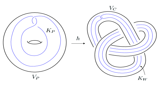
Let $K_{P}$ be a non-trivial knot in $S^{3}$ and $V_{P}$ an unknotted solid torus in $S^{3}$ with $K_{P}\subset V_{P}\subset S^{3}$. Let $K_{C}\subset S^{3}$ be another knot and let $V_{C}$ be a tubular neighborhood of $K_{C}$ in $S^{3}$. Let $h:V_{P}\to V_{C}$ be a homeomorphism and let $K_{W}$ be $h(K_{P})$. We say $K_{C}$ is a companion of any knot $K_{W}$ constructed (up to knot type) in this manner. If $h$ is faithful, meaning that $h$ takes the preferred longitude and meridian of $V_{P}$ respectively to the preferred longitude and meridian of $V_{C}$, We say $K_{W}$ is an untwisted Whitehead double of $K_{C}$. Otherwise, $K_{W}$ is a twisted Whitehead double. For instance, Figure 3 is a 3-twisted Whitehead double of a trefoil knot. The pair $(V_{P},K_{P})$ is the pattern of $K_{W}$.

Figure 3. A 3-twisted Whitehead double of a trefoil knot

The second tool is based on a type of connected sum of a pair of manifolds $(M_{1}^{m},N_{1}^{n})\#(M_{2}^{m},N_{2}^{n})$, where $N_{i}^{n}$ is a locally flat submanifold of $M_{i}^{m}$. Treat the above pair as $(S^{3},k_{1})\#(S^{3},k_{2})$ where $k_{i}$ are tame knots. Removing a standard ball pair $(B_{i}^{3},B_{i}^{1})$ from $(S^{3},k_{1})$ and gluing the resulting pairs by a homeomorphism $h:(\partial B_{2}^{3},\partial B_{2}^{1})\to(\partial B_{1}^{3},\partial B_{1}^{1})$ to form the pair connected sum. For convenience, we use $k_{1}\#k_{2}$ other than pairs of manfolds. See [Rol76] for details.

To help readers get a better feeling about group $\pi_{1}(K_{j})$, we show that $\pi_{1}(K_{j})$ is isomorphic to $\pi_{1}\left((T_{j}\backslash\operatorname{Int}h_{j}^{0}(T_{0}))/\partial T_{j}\right)$. Geometrically, $K_{j}$ is the space obtained by sewing the solid torus $S^{3}\backslash\operatorname{Int}T_{j}$ to $T_{j}\backslash\operatorname{Int}h_{j}^{0}(T_{0})$ along $\partial T_{j}$. We decompose $S^{3}\backslash\operatorname{Int}T_{j}$ into two 3-cells $B_{1}$ and $B_{2}$, i.e., $S^{3}\backslash\operatorname{Int}T_{j}=B_{1}\cup B_{2}$, where $B_{1}$ is the thickened meridional disk $D$ in $S^{3}\backslash\operatorname{Int}T_{j}$ with $\partial D=\alpha_{j}$ (see Figure 4) and $B_{2}$ is the closure of the complement of $B_{1}$ in $S^{3}\backslash\operatorname{Int}T_{j}$. Sewing $B_{1}$ to $T_{j}\backslash\operatorname{Int}h_{j}^{0}(T_{0})$ along an annular neighborhood of $\alpha_{j}$ in $\partial T_{j}$. By Seifert-van Kampen, the inclusion $T_{j}\backslash\operatorname{Int}h_{j}^{0}(T_{0})\hookrightarrow(T_{j}\backslash\operatorname{Int}h_{j}^{0}(T_{0}))\cup B_{1}$ induces a surjection on fundamental groups whose kernel is the normal closure of the curve $\alpha_{j}$ in $\pi_{1}(T_{j}\backslash\operatorname{Int}h_{j}^{0}(T_{0}))$.

Figure 4. $\beta_{j}$ contracts in $S_{j-1}^{3}\backslash\operatorname{Int}h_{j}^{0}(T_{0})$, where $h_{j}^{0}(T_{0})$ is not pictured.

Adding $B_{2}$ to $(T_{j}\backslash\operatorname{Int}h_{j}^{0}(T_{0}))\cup B_{1}$ to form the knot complement $K_{j}$ does not affect the fundamental group. This follows readily from Seifert-van Kampen. Hence, the inclusion $T_{j}\backslash\operatorname{Int}h_{j}^{0}(T_{0})\hookrightarrow K_{j}$ induces a surjection on fundamental groups whose kernel is the normal closure of the curve $\alpha_{j}$ in $\pi_{1}(T_{j}\backslash\operatorname{Int}h_{j}^{0}(T_{0}))$.

Claim 2.

$\pi_{1}(K_{j})$ is isomorphic to $\pi_{1}\left((T_{j}\backslash\operatorname{Int}h_{j}^{0}(T_{0}))/\partial T_{j}\right)$.

Proof.

It’s sufficient to show that the meridian $\beta_{j}$ of $T_{j}$ is trivial in $\pi_{1}(K_{j})$. In other words, we will show that $\beta_{j}$ contracts in the complement of $h_{j}^{0}(T_{0})$. Consider Figure 4. $h_{j}^{0}(T_{0})$ (not pictured) is contained in $h_{j}^{j-1}(T_{j-1})$, which is also contained in the solid torus $A$. Since $A$ is an unknotted solid torus, $\beta_{j}$ bounds a 2-chain in $S^{3}\backslash A$. ∎

It’s clear that $\pi(K_{1})$ is isomorphic to a trefoil knot group.

Claim 3.

$\pi_{1}(K_{2})$ is isomorphic to the knot group of the connected sum of a trefoil knot and a $3$-twisted Whitehead double of a trefoil knot.

Proof.

By the construction of $W^{3}$, $T_{1}^{*}$ embeds in $T_{2}^{*}$ just as the way $T_{0}^{*}$ embeds in $T_{1}^{*}$ (as shown in Figure 1). Note that the space $K_{2}=S^{3}\backslash\operatorname{Int}h_{2}^{0}(T_{0})$ can be decomposed into

$$(S^{3}\backslash\operatorname{Int}T_{2}^{*})\cup(T_{2}^{*}\backslash\operatorname{Int}T_{1}^{*})\cup(T_{1}^{*}\backslash\operatorname{Int}T_{0}^{*}).$$

Since a solid torus $S^{3}\backslash\operatorname{Int}T_{2}^{*}$ is glued to $T_{2}^{*}\backslash\operatorname{Int}T_{1}^{*}$ along $\partial T_{2}^{*}$, one can unlink the clasped portion of $T_{1}^{*}$ while keeping the way $T_{0}^{*}$ embeds in $T_{1}^{*}$ via an ambient isotopy $\Psi_{t}$ of $S^{3}$ starting at $\Psi_{0}=\operatorname{Id}_{S^{3}}$. The restriction $\Psi_{1}(T_{1}^{*})$ is a tubular neighborhood of a trefoil knot, denoted $\mathcal{K}_{*}$. Name a twisted Whitehead double of $\mathcal{K}_{*}$ (as shown in Figure 3) $\mathcal{K}_{*}^{Wh}$. Restrict $\Psi_{1}$ to $T_{0}^{*}$ and deformation retract $\Psi_{1}(T_{0}^{*})$ onto its core. The core of $\Psi_{1}(T_{0}^{*})$ is $\mathcal{K}_{*}^{Wh}$ connected sum with a small trefoil knot, denoted $\mathcal{K}_{**}$. Consider the knot of Figure 5. In this case, $\mathcal{K}_{1}^{Wh}$ is $\mathcal{K}_{*}^{Wh}$ and $\mathcal{K}_{1}$ is $\mathcal{K}_{**}$. It follows easily that $K_{2}$ is homotopy equivalent to $S^{3}\backslash(\mathcal{K}_{*}^{Wh}\#\mathcal{K}_{**})$. ∎

Figure 5. The connected sum of a twisted Whitehead double of $\mathcal{K}_{1}$ and $\mathcal{K}_{1}(\approx$ trefoil knot). Here “$\approx$” stands for homeomorphic.

Let $\mathcal{K}_{1}$ be a trefoil knot corresponding to the knot space $K_{1}$. Denote a knot $\mathcal{K}_{2}$ by $\mathcal{K}_{1}^{Wh}\#\mathcal{K}_{1}$ such that $\pi_{1}(S^{3}\backslash\mathcal{K}_{2})\cong\pi_{1}(K_{2})$. Similarly, one can further find a knot $\mathcal{K}_{3}$ on the 3rd stage which is a connected sum of a twisted Whitehead double of $\mathcal{K}_{2}$ and $\mathcal{K}_{1}$. By iteration, a knot $\mathcal{K}_{j}$ can be viewed as $\mathcal{K}_{j-1}^{Wh}\#\mathcal{K}_{1}$.

Let $G_{3_{1}}$ and $G^{Wh}_{j-1}$ be the knot group of $\mathcal{K}_{1}$ and $K^{Wh}_{j-1}$ respectively. By the definition of connected sum, there is a tame 2-sphere $S^{2}$ dividing $S^{3}$ into two balls $B_{Wh}$ and $B_{1}$ containing $K^{Wh}_{j-1}$ and $\mathcal{K}_{1}$ respectively. The intersection of $K^{Wh}_{j-1}$ and $\mathcal{K}_{1}$ is an arc $\zeta$ lying in $S^{2}$. View $\mathcal{K}_{j}=K^{Wh}_{j-1}\#\mathcal{K}_{1}$ as the union of $K^{Wh}_{j-1}$ and $\mathcal{K}_{1}$ minus $\operatorname{Int}\zeta$ (see Figure 5). Then we have the following diagram “pushout” commutative diagram 6.

Figure 6. “Pushout” commutative diagram

Clearly, the two upper homomorphisms in Figure 6 are injective. By the Seifert-van Kampen theorem, the other two homomorphisms $\iota_{1},\iota_{2}$ are also injective. That means

$$G_{j}=\pi_{1}(S^{3}\backslash\mathcal{K}_{j})=G^{Wh}_{j-1}\ast_{\langle\lambda\rangle}G_{3_{1}}$$

is a free product with amalgamation along an infinite cyclic group, where $[\lambda]$ corresponds to the loop class in $\pi_{1}(S^{2}\backslash\mathcal{K}_{j})$. According to this set-up, $G^{Wh}_{j-1}$ and $G_{3_{1}}$ are two subgroups of $G_{j}$ and $\langle\lambda\rangle$ is a subgroup of both $G^{Wh}_{j-1}$ and $G_{3_{1}}$. Since both $G^{Wh}_{j-1}$ and $G_{3_{1}}$ are abelianized to $\langle\lambda\rangle\cong\mathbb{Z}$, $G_{j}$ is a split amalgamated free product. Although the work in [Wei99] guarantees a lower bound for $\operatorname{Rank}G_{j}\ast_{\langle\lambda\rangle}G_{3_{1}}$, i.e., $\operatorname{Rank}G_{j}\ast_{\langle\lambda\rangle}G_{3_{1}}\geq 2$, the ultimate goal is to show that $\operatorname{Rank}G_{j}\ast_{\langle\lambda\rangle}G_{3_{1}}$ has no upper bound as $j\to\infty$. At the time of writing, we don’t know whether there is a direct knot theoretical approach to this. So, we use the covering space theory as developed by Sternfeld in [Ste77].

We start by constructing a surjective homomorphism $\Phi_{j}:G^{Wh}_{j-1}\ast_{\langle\lambda\rangle}G_{3_{1}}\twoheadrightarrow\mathbb{A}_{5}$, where $\mathbb{A}_{5}$ is an alternating group on 5 letters. To that end, by the definition of $W^{3}$, we decompose $K_{j}$ into an amalgamation of $L_{j}$’s. That is, for $j\geq 1$,

(2.1) $$K_{j}\approx(S^{3}\backslash\operatorname{Int}T_{j})\cup_{\operatorname{Id}}L_{j}\cup_{h_{j}^{j-1}}L_{j-1}\cup_{h_{j-1}^{j-2}}\cdots\cup_{h_{2}^{1}}L_{1},$$

where the sewing homeomorphism $h_{l+1}^{l}$ identifies the boundary component $\partial T_{l}$ of $L_{l}$ to the boundary component $\partial T^{\prime}_{l+1}$ of $L_{l+1}$. It’s clear that $\pi_{1}(K_{j})\cong G_{j}$. So, we convert the problem to finding a surjection from $\pi_{1}(K_{j})\to\mathbb{A}_{5}$ which will be discussed in the following two sections.

3. A presentation of $\pi_{1}(K_{j})$

First we spell out a Wirtinger presentation similar to what Sternfeld did in [Ste77, P.20–26] for $\pi_{1}(L_{l})$, where $l\geq 1$. Let $\Sigma_{l}$ and $\Omega_{l}$ be polyhedral simple closed curves contained in $S^{3}$ such that $S^{3}\backslash(\Sigma_{l}\cup\Omega_{l})$ deformation retracts onto $L_{l}$. $\Sigma_{l}$ and $\Omega_{l}$ can be viewed as cores of the solid tori $T_{l}^{\prime}$ and $S^{3}\backslash\operatorname{Int}T_{l}$ respecitively (see Figures 1 and 7). Let the arc $\mu_{l}$ in Figure 7 run from one end point $p_{l}\in\partial T_{l}^{\prime}$ and to the other end point $q_{l}\in\partial T_{l}$. $\mu_{l}$ is properly embedded in $L_{l}$.

Figure 7. A Projection of $\Sigma_{l}\cup\Omega_{l}$ into the plane. Arrows $a,b,c,\dots,i$ have subscript $l$ corresponding to $L_{l}$ ($1<l\leq j$) is suppressed.

Hence, the presentation of $\pi_{1}(S^{3}\backslash(\Sigma_{l}\cup\Omega_{l}),p_{l})$ is

(3.1) $$\text{Generators: }a,b,c,\dots,i$$

$$\text{Relators:}\begin{cases}\begin{aligned} R_{l,1}:b&=c^{-1}ac\\ R_{l,2}:c&=a^{-1}ba\\ R_{l,3}:d&=b^{-1}cb\\ R_{l,4}:e&=gdg^{-1}\\ R_{l,5}:f&=heh^{-1}\\ R_{l,6}:g&=efe^{-1}\\ R_{l,7}:a&=h^{-1}gh\\ R_{l,8}:h&=g^{-1}ig\\ R_{l,9}:i&=fhf^{-1},\end{aligned}\end{cases}$$

where the subscripts $l$’s are surpressed.

Write loop classes $[\alpha_{l}],[\beta_{l}],[\gamma_{l}]$ and $[\delta_{l}]$ as words in the generators $a_{l},b_{l},\dots,i_{l}$ of (3.1):

(3.2) $$\begin{cases}\begin{aligned} &[\alpha_{l}]=h_{l}\\ &[\beta_{l}]=f_{l}^{-1}g_{l}\\ &[\gamma_{l}]=a_{l}\\ &[\delta_{l}]=c_{l}a_{l}b_{l}g_{l}^{-1}h_{l}^{-1}e_{l}^{-1}h_{l}\\ \end{aligned}\end{cases}$$

where $[\alpha_{l}]$ is determined by the oriented simple closed curve $\alpha_{l}$ lying in $\partial L_{l}$ (see Figures 1 and 7) and the arc $\mu_{l}$ connecting $\alpha_{l}$ to the base point $p_{l}$. Likewise, $[\beta_{l}]$, $[\gamma_{l}]$ and $[\delta_{l}]$ are defined in the same manner. Deformation retract $S^{3}\backslash(\Sigma_{l}\cup\Omega_{l})$ onto $L_{l}$. It’s clear that Presentation (3.1) is a presentation of $\pi_{1}(L_{l},p_{l})$. Consider the loop classes $a_{l},b_{l},\dots,i_{l}$ in $\pi_{1}(L_{l},p_{l})$ (represented by the same loops as before) as loops in $L_{l}$. At the same time, $[\alpha_{l}],[\beta_{l}],[\gamma_{l}]$ and $[\delta_{l}]$ may be written as the same words (3.2) in the generators of $\pi_{1}(L_{l},p_{l})$.

Recall in the previous section, we have the following knot space

$$K_{j}\approx(S^{3}\backslash\operatorname{Int}T_{j})\cup_{\operatorname{Id}}L_{j}\cup_{h_{j}^{j-1}}L_{j-1}\cup_{h_{j-1}^{j-2}}\cdots\cup_{h_{2}^{1}}L_{1},$$

where the sewing homeomorphism $h_{l+1}^{l}$ identifies the boundary component $\partial T_{l}$ of $L_{l}$ to the boundary component $\partial T^{\prime}_{l+1}$ of $L_{l+1}$ such that the transverse oriented simple closed curves $\alpha_{l}$ and $\beta_{l}$ of $\partial T_{l}$ are mapped in an orientation preserving manner to the transverse oriented simple closed curves $\delta_{l+1}$ and $\gamma_{l+1}$ respectively in $\partial T^{\prime}_{l+1}$. Using the words (3.2), this can be described by the following relators

(3.3) $$\text{Relators}\begin{cases}\begin{aligned} &S_{l,1}:h_{l-1}=c_{l}a_{l}b_{l}g_{l}^{-1}h_{l}^{-1}e_{l}^{-1}h_{l}\text{ for }j\geq l\geq 2\\ &S_{l,2}:f_{l-1}^{-1}g_{l-1}=a_{l}\text{ for }j\geq l\geq 2.\\ \end{aligned}\end{cases}$$

Combine the words (3.1) and (3.3), we obtain

Proposition 3.1.

$\pi_{1}(K_{j},p_{1})$, $j\geq 1$, has the following presentation

(3.4) $$\text{Generators: }a_{l},b_{l},c_{l},\dots,i_{l}\text{ for }j\geq l\geq 1$$

$$\text{Relators:}\begin{cases}\begin{aligned} &R_{l,k}\text{ for }j\geq l\geq 1\text{ and }9\geq k\geq 1\\ &S_{l,1}\text{ for }j\geq l\geq 2\\ &S_{l,2}\text{ for }j\geq l\geq 2\\ &h_{j}=1,\end{aligned}\end{cases}$$

where the generators $a_{l},\dots,i_{l}$ of Presentation (3.4) correspond to those of Presentation (3.1) conjugated by the path $\mu_{l}$.

Proof.

The proof is an easy modification of the proof of Proposition 4.1 in [Ste77]. ∎

4. The surjection of $\pi_{1}(K_{j},p_{1})$ onto $\mathbb{A}_{5}$

Here we shall define a homomorphism $\Phi_{j}:\pi_{1}(K_{j},p_{1})\to\mathbb{A}_{5}$, where $j\geq 1$. It suffices to define $\Phi_{j}$ on the generators of Presentation (3.4) of $\pi_{1}(K_{j},p_{1})$ and check that the definition is compatible with the relators of the presentation. That is, if the following words

$$w(a_{1},b_{1},\dots,i_{1},\dots,a_{j},b_{j},\dots,i_{j})=w^{\prime}(a_{1},b_{1},\dots,i_{1},\dots,a_{j},b_{j},\dots,i_{j})$$

is a relator of the presentation, then

$$w(\Phi_{1}(a_{1}),\dots,\Phi_{1}(i_{1}),\dots,\Phi_{j}(a_{j}),\dots,\Phi_{j}(i_{j}))=w^{\prime}(\Phi_{1}(a_{1}),\dots,\Phi_{1}(i_{1}),\dots,\Phi_{j}(a_{j}),\dots,\Phi_{j}(i_{j}))$$

must hold for $\mathbb{A}_{5}$.

Consider an extreme case by “unknotting” every small trefoil knot in the link (corresponding to $L_{l}$) as shown in Figure 7. The link in Figure 7 can be viewed as a connected sum of a Whitehead link and a trefoil knot. Thus, we can abelianize the trefoil knot group to $\langle a_{l}\rangle$ while keeping the remaining structure of the group of the link complement fixed. Inherit the definitions of $T_{l}$, $T^{\prime}_{l}$ and $h_{l+1}^{l}$ in constructing the knot space $K_{j}$. Unknot the trefoil-knotted hole in $C_{l}$ when we embed $T^{\prime}_{l}$ into $T_{l}$. For convenience, we still call such reembedded torus $T^{\prime}_{l}$. Similar to the construction of the knot space $K_{j}$, the sewing homeomorphism $h_{l+1}^{l}$ identifies the boundary component $\partial T_{l}$ of $L_{l}$ to the boundary component $\partial T^{\prime}_{l+1}$ of $L_{l+1}$ such that the transverse oriented simple closed curves $\alpha_{l}$ and $\beta_{l}$ of $\partial T_{l}$ are mapped in an orientation preserving manner to the transverse oriented simple closed curves $\delta_{l+1}$ and $\gamma_{l+1}$ respectively in $\partial T^{\prime}_{l+1}$. Furthermore, when $\alpha_{l}$ of $\partial T_{l}$ is mapped to $\delta_{l+1}$ in $\partial T^{\prime}_{l+1}$, $h_{l+1}^{l}$ first gives 3 compensating half-twists to $T_{l}$ due to the writhe of trefoil knot (before abelianization) in $T^{\prime}_{l+1}$ is 3. In other words, the new knot space is a concatenation of Whitehead links with 3 half-twists. Denote the corresponding knot space by $K_{j}^{**}$. By the above procedure, $\pi_{1}(K_{j}^{**})$ can be obtained by adding relators $a_{l}=b_{l}$, $b_{l}=c_{l}$ and $c_{l}=d_{l}$ to the presentation of $\pi_{1}(K_{j})$ in Proposition 3.1

(4.1) $$\text{Generators: }a_{l},b_{l},c_{l},\dots,i_{l}\text{ for }j\geq l\geq 1$$

$$\text{Relators:}\begin{cases}\begin{aligned} &a_{l}=b_{l},b_{l}=c_{l},c_{l}=d_{l}\\ &R_{l,k}\text{ for }j\geq l\geq 1\text{ and }9\geq k\geq 1\\ &S_{l,1}\text{ for }j\geq l\geq 2\\ &S_{l,2}\text{ for }j\geq l\geq 2\\ &h_{j}=1.\end{aligned}\end{cases}$$

Clearly, there is a surjection of $\psi_{j}:\pi_{1}(K_{j})\twoheadrightarrow\pi_{1}(K_{j}^{**})$ by sending $a_{l},\dots,d_{l}$ in Presentation (3.4) to $a_{l}$ in Presentation (4.1). So, it suffices to find a surjection $\phi_{j}$ of $\pi_{1}(K_{j}^{**})$ onto $\mathbb{A}_{5}$.

We shall define $\phi_{j}$ inductively on the generators of Presentation (4.1). If $j=1$, we use GAP [GAP18] to define a surjection $\phi_{1}$ on $a_{1},\dots,i_{1}$ by Table 1a. This definition is compatible with the relators $R_{1,k}$ and $h_{1}=1$, where $1\leq k\leq 9$. If $j=2$, both Tables 1a and 1b are used. Besides relators $R_{1,k},R_{2,k}$ and $h_{2}=1$, relators $S_{2,1}$ and $S_{2,2}$ are also compatible. Similarly, if $j=3$ (resp. $j=4$), Tables 1a-1c (resp. 1a-2a) are applied. When $j\geq 5$, Tables 1a-2b will be applied periodically. That is, extend $\phi_{j}$ to the generators $a_{l},\dots,i_{l}$ according to Table 1a if $l=j$, according to Table 1b if $l=j-1-4T$, according to Table 1c if $l=j-2-4T$, according to Table 2a if $l=j-3-4T$ and according to Table 2b if $l=j-4-4T$, where $T\in\mathbb{N}$ and $0\leq T\leq(j-1)/4$. One can either use GAP [GAP18] or simply by hand to check such extension is compatible with relators in Presentation (3.4). Hence, the composition $\Phi_{j}=\phi_{j}\circ\psi_{j}$ is the desired surjection.

Table 1.

Generators	Image
$a_{l}$	(1,2)(3,4)
$b_{l}$	(1,2)(3,4)
$c_{l}$	(1,2)(3,4)
$d_{l}$	(1,2)(3,4)
$e_{l}$	(1,2)(3,4)
$f_{l}$	(1,2)(3,4)
$g_{l}$	(1,2)(3,4)
$h_{l}$	()
$i_{l}$	()

(a) $l=j$

Generators	Image
$a_{l}$	(1,2,3)
$b_{l}$	(1,2,3)
$c_{l}$	(1,2,3)
$d_{l}$	(1,2,3)
$e_{l}$	(2,4,3)
$f_{l}$	(1,3,4)
$g_{l}$	(1,4,2)
$h_{l}$	(1,2)(3,4)
$i_{l}$	(1,3)(2,4)

(b) $l=j-1-4T$

Generators	Image
$a_{l}$	(1,3)(4,5)
$b_{l}$	(1,3)(4,5)
$c_{l}$	(1,3)(4,5)
$d_{l}$	(1,3)(4,5)
$e_{l}$	(1,2)(4,5)
$f_{l}$	(1,3)(4,5)
$g_{l}$	(2,3)(4,5)
$h_{l}$	(1,2,3)
$i_{l}$	(1,3,2)

(c) $l=j-2-4T$

Table 2.

Generators	Image
$a_{l}$	(3,4,5)
$b_{l}$	(3,4,5)
$c_{l}$	(3,4,5)
$d_{l}$	(3,4,5)
$e_{l}$	(1,3,5)
$f_{l}$	(1,4,3)
$g_{l}$	(1,5,4)
$h_{l}$	(1,3)(4,5)
$i_{l}$	(1,5)(3,4)

(a) $l=j-3-4T$

Generators	Image
$a_{l}$	(1,2)(3,4)
$b_{l}$	(1,2)(3,4)
$c_{l}$	(1,2)(3,4)
$d_{l}$	(1,2)(3,4)
$e_{l}$	(1,2)(4,5)
$f_{l}$	(1,2)(3,4)
$g_{l}$	(1,2)(3,5)
$h_{l}$	(3,4,5)
$i_{l}$	(3,5,4)

(b) $l=j-4-4T$

Remark 2.

In line 16 [Ste77, P.28], the author claims that the definition of $\Phi_{i}:\pi_{1}(A_{i})\to A$ given in Table 1 [Ste77, P.29] is compatible with the relators $S_{j,1},S_{j,2}$ for $l\geq j\geq 2$, where $A$ is an alternating group on 5 letters $v$, $w$, $x$, $y$ and $z$. However, for $l<i$, $\Phi(o_{l-1}^{-1}h_{l-1}f_{l-1}^{-1}q_{l-1})$ is not equal to $\Phi(a_{l})$. That is, using Table 1 [Ste77, P.29], $\Phi(o_{l-1})=(vy)(wz)$, $\Phi(h_{l-1})=(vy)(xz)$, $\Phi(f_{l-1})=(wx)(yz)$ and $\Phi(q_{l-1})=(vw)(yz)$. Hence, $\Phi(o_{l-1}^{-1}h_{l-1}f_{l-1}^{-1}q_{l-1})=(vw)(xz)=\Phi(r_{l})\neq\Phi(a_{l})=(vw)(xy)$. That means the definition of the so claimed $\Phi_{i}$ is not compatible with the relators $S_{j,1},S_{j,2}$ for $l\geq j\geq 2$. This error directly affects the following statement [Ste77, P.52]: “The composition $\pi_{1}(C_{j},x_{j})\xrightarrow{k_{\ast}}\pi_{1}(A_{i},x_{j})\xrightarrow{M_{j}}\pi_{1}(A_{i},x_{i})\xrightarrow{\Phi_{i}}A$ has image isomorphic to $\mathbb{Z}_{2}$ in $A$ since $\Phi_{i}$ maps $a_{j}$ and $b_{j}$ to the same element of order 2 in $A$. Thus, the kernel of $\Phi_{i}\circ M_{j}\circ k_{\ast}$ has index 2 in $\pi_{1}(C_{j},x_{j})$.” To fix this error, we provide a series of correct tables here.

We have to use at least 3 tables (instead of 2 tables) such that the definition of $\Phi_{i}$ is compatible with all the relators. Similar to how we define a surjection of $\pi_{1}(K_{j},p_{1})\to\mathbb{A}_{5}$ in the beginning of this section, with the assistance of GAP [GAP18], the following tables provide a surjection of $\Phi_{i}:\pi_{1}(A_{i},x_{1})\twoheadrightarrow\mathbb{A}_{5}$. If $i=1$, we defined $\Phi_{i}$ on $a_{1},\dots,u_{1}$ by Table 3a. If $i=2$, then Tables 3a and 3b are used. Otherwise, when $i\geq 3$, Tables 3a, 3b and 3c are applied. That is, extend $\Phi_{i}$ to the generators $a_{l},\dots,u_{l}$ according to Table 3a if $l=i$, according to Table 3b at $l=i-1-2T$ and according to Table 3c at $l=i-2-2T$, where $T\in\mathbb{N}$ and $0\leq T\leq(i-1)/2$.

Table 3.

Generators	Image
$a_{l}$	(1,2)(3,5)
$b_{l}$	(1,2)(3,5)
$c_{l}$	(1,2)(3,5)
$d_{l}$	(1,2)(3,5)
$e_{l}$	(1,2)(4,5)
$f_{l}$	(1,2)(4,5)
$g_{l}$	(1,2)(4,5)
$h_{l}$	(1,2)(3,5)
$i_{l}$	(1,2)(3,5)
$j_{l}$	(1,2)(4,5)
$k_{l}$	(1,2)(3,4)
$l_{l}$	(1,2)(4,5)
$m_{l}$	(1,2)(3,4)
$n_{l}$	(1,2)(3,4)
$o_{l}$	(1,2)(3,4)
$p_{l}$	(1,2)(3,4)
$q_{l}$	(1,2)(3,5)
$r_{l}$	()
$s_{l}$	()
$t_{l}$	()
$u_{l}$	()

(a) $l=i$

Generators	Image
$a_{l}$	(1,2)(4,5)
$b_{l}$	(1,2)(4,5)
$c_{l}$	(1,2)(4,5)
$d_{l}$	(1,2)(4,5)
$e_{l}$	(1,3)(4,5)
$f_{l}$	(2,5)(3,4)
$g_{l}$	(1,5)(2,4)
$h_{l}$	(1,4)(3,5)
$i_{l}$	(2,4)(3,5)
$j_{l}$	(1,3)(2,5)
$k_{l}$	(2,3)(4,5)
$l_{l}$	(1,3)(4,5)
$m_{l}$	(1,3)(4,5)
$n_{l}$	(1,5)(2,4)
$o_{l}$	(1,4)(2,3)
$p_{l}$	(1,5)(2,3)
$q_{l}$	(1,2)(3,4)
$r_{l}$	(1,2)(3,5)
$s_{l}$	(1,2)(4,5)
$t_{l}$	(1,5)(2,3)
$u_{l}$	(2,5)(3,4)

(b) $l=i-1-2T$

Generators	Image
$a_{l}$	(1,2)(3,5)
$b_{l}$	(1,2)(3,5)
$c_{l}$	(1,2)(3,5)
$d_{l}$	(1,2)(3,5)
$e_{l}$	(1,4)(3,5)
$f_{l}$	(2,5)(3,4)
$g_{l}$	(1,5)(2,3)
$h_{l}$	(1,3)(4,5)
$i_{l}$	(2,3)(4,5)
$j_{l}$	(1,4)(2,5)
$k_{l}$	(2,4)(3,5)
$l_{l}$	(1,4)(3,5)
$m_{l}$	(1,4)(3,5)
$n_{l}$	(1,5)(2,3)
$o_{l}$	(1,3)(2,4)
$p_{l}$	(1,5)(2,4)
$q_{l}$	(1,2)(3,4)
$r_{l}$	(1,2)(4,5)
$s_{l}$	(1,2)(3,5)
$t_{l}$	(1,5)(2,4)
$u_{l}$	(2,5)(3,4)

(c) $l=i-2-2T$

5. Properties of a cube with a trefoil-knotted hole

One of the key ingredients in proving Theorem 1.1 is to understand the covering space of a cube with a trefoil-knotted hole as shown in Figure 1. In this section, we collect a number of important properties about cubes with a trefoil-knotted hole. Let $C$ be the cube with a trefoil-knotted hole as shown in Figure 8. Here $C$ is the complement in $S^{3}$ of the interior of a regular neighborhood of the polyhedral simple closed curve $\Gamma$. There is a deformation retract of $S^{3}\backslash\Gamma$ onto $C$. The presentation of $\pi_{1}(S^{3}\backslash\Gamma)$ (i.e., trefoil knot group) is a presentation of $\pi_{1}(C,p_{0})$, where $p_{0}$ is a base point. Hence, one can use the Wirtinger presentation of $\pi_{1}(S^{3}\backslash\Gamma)$ to obtain the following proposition.

Figure 8. The Cube-With-trefoil-Knotted Hole. $C$ is the complement in $S^{3}$ of the interior of a regular neighborhood of the trefoil-knotted simple closed curve $\Gamma$

Proposition 5.1.

$\pi_{1}(C,p_{0})$ has presentation

$$\langle a,b|b^{-1}a^{-1}b^{-1}aba=1\rangle,$$

where $a=[A]$ and $b=[B]$ as shown in Figure 8.

Corollary 5.2.

$\pi_{1}(C,p_{0})$ has $\operatorname{Rank}2$.

Proof.

Obviously, $\operatorname{Rank}\pi_{1}(C,p_{0})\leq 2$. By the classification of finite simple groups, $\operatorname{Rank}\mathbb{A}_{5}=2$. Using GAP [GAP18], one can find a surjection of $\pi_{1}(C,p_{0})$ onto $\mathbb{A}_{5}$ by $(a,b)\mapsto\big{(}(1,3,5,4,2),(1,2,3,4,5)\big{)}$. That means $\operatorname{Rank}\pi_{1}(C,p_{0})$ has to be greater or equal to 2. Hence, $\operatorname{Rank}\pi_{1}(C,p_{0})=2$. ∎

Proposition 5.3.

[Ste77, Prop.6.3] $C$ has a unique $2$-fold cover, $\tilde{C}^{2}$, the boundary $\partial\tilde{C}^{2}$ is connected and the quotient map

$$Q:\tilde{C}^{2}\to\tilde{C}^{2}/\partial\tilde{C}^{2}$$

induces a surjection on fundamental groups.

Lemma 5.4.

[Ste77, Lemma 1.3] Let $B$ be a subspace of $X$. Let $B$ and $X$ be path connected. If $B$ is collared in $X$, then the quotient map $q:X\to X/B$ induces a surjection of fundamental groups whose kernel is the normal closure in $\pi_{1}(X)$ of $i_{\ast}\pi_{1}(B)$, where $i_{*}$ denotes the inclusion induced homomorphism.

The following result generalizes Proposition 5.3 for the $k$-fold cyclic cover of $C$.

Proposition 5.5.

Let $\tilde{C}^{k}$ be the $k$-fold cyclic cover of $C$. Then $\partial\tilde{C}^{k}$ is connected and the quotient map

$$Q:\tilde{C}^{k}\to\tilde{C}^{k}/\partial\tilde{C}^{k}$$

induces a surjection on fundamental groups.

Proof.

First, we show $\partial\tilde{C}^{k}$ is connected. Let $P:\tilde{C}^{k}\to C$ be the $k$-fold cyclic cover. The restriction of $P$ to each component of $P^{-1}(\partial C)$ is a covering map of $\partial C$. Note that the $k$-fold cyclic cover is defined to be the one which corresponds to the kernel of the composite

$$\pi_{1}(C)\xrightarrow{abelianization}\mathbb{Z}\xrightarrow{projection}\mathbb{Z}_{k}.$$

The uniqueness of the abelianization and the projection assures that the simple closed curve $A$ (see Figure 8) in $\partial C$ based at a point $p_{0}$ has a lift $\tilde{A}$ which is not a loop since the loop $[A]$ corresponding to the generator $a$ in Proposition 5.1 is not in the kernel. Therefore, the component of $\partial\tilde{C}^{k}$ that contains $\tilde{A}$ must be a least a double cover of $\partial C$ since the two end points of $\tilde{A}$ cover $p_{0}$. Since each point of $C$ has precisely $k$ preimages in $\tilde{C}^{k}$, the component of $\partial\tilde{C}^{k}$ that contains $\tilde{A}$ must be all of $\partial\tilde{C}^{k}$. Thus $\partial\tilde{C}^{k}$ is (path) connected.

Applying Lemma 5.4 finishes the proof. ∎

Proposition 5.6.

$\pi_{1}(\tilde{C}_{2}/\partial\tilde{C}_{2})\cong\mathbb{Z}_{3}.$

Proof.

The proof is a standard covering space argument. See the proof of Prop.6.4 in [Ste77, P.39-46]. ∎

Proposition 5.7.

Let $\tilde{C}^{3}$ be the $3$-fold cyclic cover of $C$. Then $\operatorname{Rank}\pi_{1}(\tilde{C}^{3}/\partial\tilde{C}^{3})\geq 1.$

Proof.

Standard cyclic cover argument [Rol76, Ch.6] assures the first homology group $H_{1}(\tilde{C}^{3})\cong\mathbb{Z}_{2}\oplus\mathbb{Z}_{2}\oplus\mathbb{Z}$. “Modulo out” the generators corresponding the boundary $\tilde{C}^{3}$ can at most reduce the rank by 2, hence, $\operatorname{Rank}\pi_{1}(\tilde{C}^{3}/\partial\tilde{C}^{3})\geq 3-2=1$. ∎

6. Proof of Theorem 1.1

Recall in Section 2 we pointed out the key in proving Theorem 1.1 is to show that $\operatorname{Rank}\pi_{1}(K_{j},p_{1})$ is not bounded. Since $\mathbb{A}_{5}$ has order 60 and $\Phi_{j}:\pi_{1}(K_{j},p_{1})\to\mathbb{A}_{5}$ is onto, $\ker\Phi_{j}$ has index 60 in $\pi_{1}(K_{j},p_{1})$. Then the following formula guarantees that it suffices to show that $\operatorname{Rank}\ker\Phi_{j}$ is not bounded.

The formula can be viewed as a corollary of the Schreier index theorem. A detailed proof by utilizing covering space theory can be found in [Ste77, Lemma 1.4].

Lemma 6.1.

Let $G$ be a group and $H$ be a subgroup of index $i$. If $\operatorname{Rank}H\geq m$, then $\operatorname{Rank}G\geq\frac{m-1}{i}+1$.

Let $P_{j}:(\tilde{K}_{j},\tilde{p}_{1})\to(K_{j},p_{1})$ be the covering map such that the induced map $P_{j\ast}:\pi_{1}(\tilde{K}_{j},\tilde{p}_{1})\to\pi_{1}(K_{j},p_{1})$ is an isomorphism onto $\ker\Phi_{j}$. By Lemma 6.1, it remains to show that $\operatorname{Rank}\ker\Phi_{j}$ is not bounded above as $j\to\infty$, which is equivalent to showing that $\operatorname{Rank}\pi_{1}(\tilde{K}_{j},\tilde{p}_{1})\geq 25j$ (resp. $5(5j+1)$) when $j$ is even (resp. odd). The key is the fact that $K_{j}$ contains $j$ pairwise disjoint incompressible cubes with trefoil-knotted hole. Figure 1 shows that each $L_{l}$, $l\geq 1$ contains a cube with trefoil-knotted hole $C_{l}$. Recall

$$K_{j}\approx(S^{3}\backslash\operatorname{Int}T_{j})\cup_{\operatorname{Id}}L_{j}\cup_{h_{j}^{j-1}}L_{j-1}\cup_{h_{j-1}^{j-2}}\cdots\cup_{h_{2}^{1}}L_{1},$$

$K_{j}$ contains $C_{1},C_{2},\dots,C_{j}$, pairwise disjoint cubes with trefoil-knotted hole. The disjointness follows from that each $C_{l}$ lies in its own $L_{l}$ and touches only the “inner” boundary of its $L_{l}$. In $K_{j}$, when we sew two adjacent $L_{l}$’s together, only the “outer” boundary of one is glued to the “inner” boundary of the next.

Next, we shall show that $C_{l}$ in $K_{j}$ has preimage under the restriction of the covering map $P_{j}$ has 30 disjoint double covers and 20 disjoint triple covers. The proof heavily relies on the argument given in [Ste77, P.50-55]. For the convenience of readers, we spell out the proof in details.

Consider $p_{l}\in C_{l}$. See Figures 7 and 8. From the Wirtinger presentation (3.4), a loop class with subscript $l$ is the class of a loop formed by conjugation of a loop in $L_{l}$ based at $p_{l}$ by the path $\mu_{l}^{1}$ running from $p_{1}$ to $p_{l}$ in $K_{j}$. Define a change-basepoint isomorphism $M_{l}:\pi_{1}(K_{j},p_{l})\to\pi_{1}(K_{j},p_{1})$ generated by conjugation by $\mu_{l}^{1}$. By Figures 1 and 7, loop classes $M_{l}^{-1}(a_{l})$, $M_{l}^{-1}(b_{l})$ can be viewed as loop classes of $\pi_{1}(C_{l},p_{l})$, where $1\leq l\leq j$. Then Figures 7-8 and Proposition 5.1 assure that the set $\{M_{l}^{-1}(a_{l}),M_{l}^{-1}(b_{l})\}$ generates $\pi_{1}(C_{l},p_{l})$.

Let $\iota_{*}:\pi_{1}(C_{l},p_{l})\to\pi_{1}(K_{j},p_{l})$ be the inclusion induced homomorphism. Combine the results from §4 to obtain the following composition

$$\pi_{1}(C_{l},p_{l})\xrightarrow{\iota_{*}}\pi_{1}(K_{j},p_{l})\xrightarrow{M_{l}}\pi_{1}(K_{j},p_{1})\xrightarrow{\Phi_{j}}\mathbb{A}_{5},$$

which has image isomorphic to $\mathbb{Z}_{2}$ (resp. $\mathbb{Z}_{3}$) in $\mathbb{A}_{5}$ when $l=j,j-2-4T$ and $j-4-4T$ (resp. $l=j-1-4T$ and $j-3-4T$). See Tables 1a, 1c and 2b (resp. 1b and 2a). That is because $\Phi_{j}$ maps $a_{l}$ and $b_{l}$ of $\pi_{1}(C_{l},p_{l})$ to the same element of order 2 (resp. 3) in $\mathbb{A}_{5}$. It follows that the kernel of $\Phi_{j}\circ M_{l}\circ\iota_{2}$ has index either 2 or 3 in $\pi_{1}(C_{l},p_{l})$. Let $q:(\tilde{C}_{l}^{2},\hat{p}_{l})\to(C_{l},p_{l})$ be a 2-fold cover of $(C_{l},p_{l})$ corresponding to the kernel.

Claim 4.

Each $\tilde{C}_{l}^{2}$ embeds in $\tilde{K}_{j}$.

Proof.

Note that there exists a lift $\tilde{p}_{l}$ of $p_{l}$ in $\tilde{K}_{j}$ so that $P_{j*}(\pi_{1}(\tilde{K}_{j},\tilde{p}_{l}))=\ker(\Phi_{j}\circ M_{l})$. The lift is obtained by lifting $\mu_{l}^{1}$ to a path $\tilde{\mu}_{l}^{1}$ so $\mu_{l}^{1}(0)=\tilde{p}_{1}$ and the point $\tilde{p}_{l}$ is defined to be $\tilde{\mu}_{l}^{1}(1)$. Since $\iota_{*}q_{*}(\pi_{1}(\tilde{C}_{l}^{2},\hat{p}_{l}))\subseteq P_{j*}(\pi_{1}(\tilde{K}_{j},\tilde{p}_{l}))$, we have the following commutative diagram with $\iota$ lifted to $\tilde{\iota}$

$$\begin{array}[c]{ccc}(\tilde{C}_{l}^{2},\hat{p}_{l})&\xrightarrow{\tilde{\iota}}&(\tilde{K}_{j},\tilde{p}_{l})\\ \downarrow q&&\downarrow P_{j}\\ (C_{l},p_{l})&\xrightarrow{\iota}&(K_{j},p_{l})\par\end{array}$$

We shall apply standard covering space theory to show $\tilde{\iota}$ is an embedding. It suffices to prove that $\tilde{\iota}$ is 1-1. Suppose $x$ and $y$ are two elements of $\tilde{C}_{l}^{2}$ such that $\tilde{\iota}(x)=\tilde{\iota}(y)$. The commutativity of the diagram above implies that $q(x)=q(y)$. Connect $x$ to $y$ by a path $\alpha$ and $x$ to $\hat{p}_{l}$ by a path $\beta$ with $\beta(0)=\hat{p}_{l}$ and $\beta(1)=x$. Lift $q(\beta)$ to $\tilde{\beta}$ so that $\tilde{\beta}(1)=y$. Suppose $x\neq y$. Then $\tilde{\beta}$ and $\beta$ are distinct lifts of $q(\beta)$. That means $\beta(0)\neq\tilde{\beta}(0)$. So, $\beta\alpha\tilde{\beta}^{-1}$ is not a loop. However, $\tilde{\iota}(\beta\alpha\tilde{\beta}^{-1})$ is a loop in $\tilde{K}_{j}$. Since $\tilde{\iota}(x)=\tilde{\iota}(y)$, $\tilde{\iota}\beta$ and $\tilde{\iota}\tilde{\beta}$ have to be the same lift of $\iota q(\beta)$. By commutativity of the diagram, $\iota q(\beta\alpha\tilde{\beta}^{-1})=P_{j}\tilde{\iota}(\beta\alpha\tilde{\beta}^{-1})$. Hence, $q(\beta\alpha\tilde{\beta}^{-1})$ is a loop in $\iota_{*}^{-1}P_{j*}(\pi_{1}(\tilde{K}_{j},\tilde{p}_{l}))$. Thus, $q(\beta\alpha\tilde{\beta}^{-1})$ must lift to a loop at $\hat{p}_{l}$. Contradiction! ∎

Remark 3.

The above argument also works for the 3-fold cover $\tilde{C}_{l}^{3}$ which will soon be defined.

Since $\tilde{\iota}$ is an embedding, $l=j,j-2-4T$ and $j-4-4T$, the restriction map $P_{j}|:\tilde{\iota}(\tilde{C}_{l}^{2})\to C_{l}$ is a 2-fold cover of $C_{l}$. Since $\ker\Phi_{j}$ has index 60 in $\pi_{1}(K_{j})$, the covering space $P_{j}:\tilde{K}_{j}\to K_{j}$ has 60 covering translations. The components of $P_{j}^{-1}(C_{l})$ are the homeomorphic images of $\tilde{\iota}(\tilde{C}_{l}^{2})$ under the 60 covering translations of $P_{j}$. Thus, every component of $P_{j}^{-1}(C_{l})$ is a 2-fold cover of $C_{l}$ (i.e., a 2-fold cover of trefoil knot). By §2, each $K_{j}$ contains $j$ pairwise disjoint cubes with trefoil-knotted hole $C_{l}$, where $1\leq l\leq j$. Hence, $\tilde{K}_{j}$ must have $15j$ (resp. $15(j+1)$) when $j$ is even (resp. odd) pairwise disjoint 2-fold covers of trefoil knot.

Likewise, let $q^{\prime}:(\tilde{C}_{l}^{3},\hat{p}_{l})\to(C_{l},p_{l})$ be a 3-fold cover of $(C_{l},p_{l})$ corresponding to the kernel of $\Phi_{j}\circ M_{l}\circ\iota_{2}$. When $l=j-1-4T$ and $j-3-4T$, the restriction map $P_{j}|:\tilde{\iota}(\tilde{C}_{l}^{3})\to C_{l}$ is a 3-fold cover of $C_{l}$.

Claim 5.

$P_{j}|:\tilde{\iota}(\tilde{C}_{l}^{3})\to C_{l}$ yields a unique $3$-fold (cyclic) cover of $C_{l}$.

Proof.

Since the 60-fold covering space of $K_{j}$ is clearly regular, the restriction of the covering projection to each $C_{l}$ is also a regular covering. Thus, the induced map $P_{j\ast}|:\tilde{\iota_{\ast}}(\pi_{1}(\tilde{C}_{l}^{3}))\to\pi_{1}(C_{l})$ goes onto an index 3 normal subgroup ($\mathbb{Z}_{3}$). Note that $\pi_{1}(\tilde{C}_{l}^{3})$ corresponds to the kernel of the composite $\pi_{1}(C_{l})\xrightarrow{abelianization}\mathbb{Z}\xrightarrow{projection}\mathbb{Z}_{3}$. Then the claim follows immediately from the uniqueness of the abelianization and the projection. ∎

When $j$ is even (resp. odd), let $D$ be the complement of the interior of the $15j$ (resp. $15(j+1)$) double covers and $10j$ (resp. $10(j-1)$) triple cover of trefoil knot in $\tilde{K}_{j}$. Let $Q_{j}:\tilde{K}_{j}\to\tilde{K}_{j}/D$ be quotient map. The quotient space $\tilde{K}_{j}/D$ is $25j$ (resp. $5(5j+1)$) when $j$ is even (resp. odd) pairwise disjoint 2-fold and 3-fold covers of trefoil knot modulo their boundaries, wedged at the point to which their boundaries are identified. By Propositions 5.6 and 5.7, $\pi_{1}(\tilde{K}_{j}/D)$ has rank at least $25j$ (resp. $5(5j+1)$) when $j$ is even (resp. odd). Then Propositions 5.3 and 5.5 assure that $Q_{j}$ induces a surjection of $\pi_{1}(\tilde{K}_{j})$ onto $\pi_{1}(\tilde{K}_{j}/D)$, hence, $\operatorname{Rank}\pi_{1}(\tilde{K}_{j})\geq 25j$ (resp. $5(5j+1)$) when $j$ is even (resp. odd).

This completes the proof of Theorem 1.1.

Proof of Theorem 1.2.

Using our building block $W^{3}$, one can apply the standard “drilling tunnel” and “piping” to generate high-dimensional examples $W^{n}$. We only spell out an outline. A detailed proof described in [Ste77, P.56-62] can readily be applied.

Recall in §3 there is an arc $\mu_{l}^{1}$ connecting the base points $p_{l}\in\partial T_{l}^{\prime}$ and $q_{l}\in\partial T_{l}$ (see Figure 7). The sewing homeomorphism $h_{l+1}^{l}$ identifies $q_{l}$ with $p_{l+1}$. By the construction of $W^{3}$, those arcs fit together to form a (base) ray $R$ in $W^{3}$. Find a regular neighborhood $N$ of $R$ such that $W^{+}=W^{3}\backslash\operatorname{Int}N$ is a PL manifold with $\partial W^{+}$ homeomorphic to $\mathbb{R}^{2}$ and $\operatorname{Int}W^{+}$ homeomorphic to $W^{3}$. The $n$-dimensional example $W^{n}$ is defined to be $W^{n}=\partial(B^{n-2}\times W^{+})=(B^{n-2}\times\partial W^{+})\cup(\partial B^{n-2}\times W^{+})$, where $B^{n-2}$ is a codimension 2 ball. The openness and contractibility follow from the standard PL topology arguments.

Define solid torus $T_{l}^{+}$ a subset of $W^{+}$ by $T_{l}^{+}=T_{l}^{*}\backslash\operatorname{Int}N$. Then $W^{+}$ can be expressed by $\cup T_{l}^{+}$. Let $p_{2}:B^{n-2}\times W^{+}\to W^{+}$ be a projection sending $B^{n-2}\times W^{+}$ onto its second factor. Let $p:W^{n}\to W^{+}$ be the restriction of $p_{2}$. Suppose there is a compact, locally connected, locally 1-connected metric space $U$ that contains $W^{n}$ as an open set. Then it suffices to show $\pi_{1}(U\backslash p^{-1}(\operatorname{Int}T_{0}^{+}))$ is not finitely generated just as how we prove Theorem 1.1. By definition of $N$, $T_{0}^{+}=T_{0}^{*}$. Let $q$ be the quotient map

$$q:T_{j}^{+}\backslash\operatorname{Int}T_{0}^{+}\to(T_{j}^{+}\backslash\operatorname{Int}T_{0}^{+})/\partial T_{j}^{+}.$$

Extend $q$ to map $Q:U\backslash p^{-1}(\operatorname{Int}T_{0}^{+})\to(T_{j}^{+}\backslash\operatorname{Int}T_{0}^{+})/\partial T_{j}^{+}$. There should be no difficult in doing so because $U\backslash p^{-1}(\operatorname{Int}T_{0}^{+})$ can be decomposed into the union of $U\backslash p^{-1}(\operatorname{Int}T_{j}^{+})$ and $p^{-1}(T_{j}^{+}\backslash\operatorname{Int}T_{0}^{+})$. Then $Q$ can be defined as the union of the constant map $l:U\backslash p^{-1}(\operatorname{Int}T_{j}^{+})\to(T_{j}^{+}\backslash\operatorname{Int}T_{0}^{+})/\partial T_{j}^{+}$ and the restriction map $q\circ p|_{p^{-1}(T_{j}^{+}\backslash\operatorname{Int}T_{0}^{+})}$. By Lemma 5.4, $q\circ p|_{p^{-1}(T_{j}^{+}\backslash\operatorname{Int}T_{0}^{+})}$ induces a surjection on fundamental groups, so does $Q$. Note that $(T_{j}^{+}\backslash\operatorname{Int}T_{0}^{+})/\partial T_{j}^{+}$ and $(T_{j}^{*}\backslash\operatorname{Int}T_{0}^{*})/\partial T_{j}^{*}$ are homeomorphic. Thus, showing that $\operatorname{Rank}\pi_{1}(U\backslash p^{-1}(\operatorname{Int}T_{0}^{+}))$ has no lower bound is equivalent to proving $\operatorname{Rank}\pi_{1}\big{(}(T_{j}^{*}\backslash\operatorname{Int}T_{0}^{*})/\partial T_{j}^{*}\big{)}=\operatorname{Rank}\pi_{1}(K_{j})$, which is just an application of Theorem 1.1. ∎

7. Questions

Recall the construction of $W^{3}$ in §2

(7.1) $$W^{3}=\lim_{j\to\infty}L_{j}\cup_{h_{j}^{j-1}}L_{j-1}\cup_{h_{j-1}^{j-2}}\cdots\cup_{h_{2}^{1}}L_{1},$$

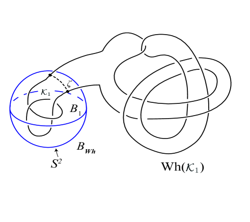
where the sewing homeomorphism $h_{l+1}^{l}$ identifies the boundary component $\partial T_{l}$ of $L_{l}$ to the boundary component $\partial T^{\prime}_{l+1}$ of $L_{l+1}$. Unknotting the cube with trefoil-knotted hole as shown in Figure 1 results in a cobordism $L^{\ast}$, which is widely known as the first stage of constructing a Whitehead manifold. See Figure 9.

Figure 9. $L^{\ast}=T\backslash T^{\prime}$. The “inner” boundary component of $L^{\ast}$ is $\partial T^{\prime}$. The “outer” boundary component of $L^{\ast}$ is $\partial T$.

Consider a variation of $W^{3}$ by placing $L^{*}$ ahead of $L_{j}$ or inserting $L^{*}$ between adjacent $L_{l}$ and $L_{l+1}$ in (7.1)

(7.2) $$W^{\ast}=\lim_{j\to\infty}L_{j}\cup_{H_{j}^{\ast}}L^{\ast}\cup_{H_{\ast}^{j-1}}L_{j-1}\cdots\cup_{h_{2}^{1}}L_{1},$$

where the sewing homeomorphism $H_{*}^{l}$ identifies the boundary component $\partial T_{l}$ of $L_{l}$ to the boundary component $\partial T^{\prime}$ of $L^{\ast}$ and the sewing homemorphism $H_{l+1}^{*}$ identifies the boundary component $\partial T$ of $L^{\ast}$ to the boundary component $\partial T^{\prime}_{l+1}$ of $L_{l+1}$. Then we obtain an infinite collection $\mathcal{C}$ by inserting $L^{*}$’s in (7.1).

The following result is an example of $\mathcal{C}$.

Proposition 7.1.

The $3$-dimensional example $W$ constructed by Sternfeld belongs to the collection $\mathcal{C}$.

Proof.

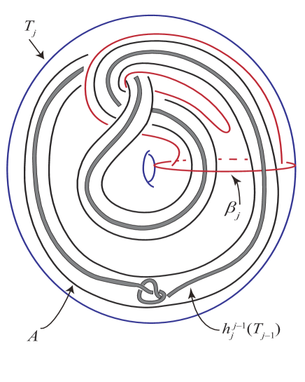
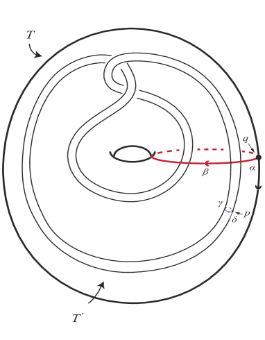
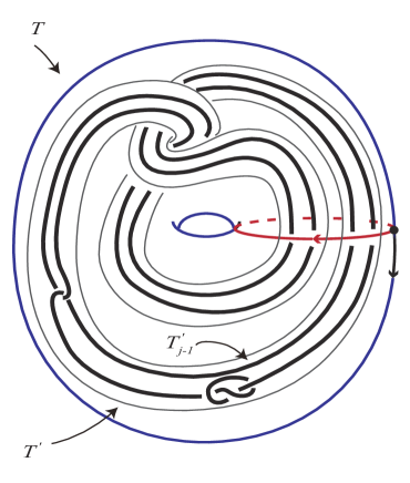
The manifold $W$ constructed by Sterneld is homeomorphic to $L^{\ast}\cup_{H_{*}^{j}}L_{j}\cup_{H_{j}^{*}}L^{\ast}\cdots$, i.e., inserting $L^{*}$ in (7.1) every other slot. See Figure 10. If one ignores the grey curves as shown in Figure 10, then the picture will be exactly the same picture given in [Ste77, P.4]. In other words, solid tori $T$ and $T_{j-1}^{\prime}$ are the first stage of Sternfeld’s construction. ∎

Remark 4.

Let $K_{j}$ and $K_{i}$ be the corresponding knot spaces of $W^{3}$ and $W$ respectively. Although both $W^{3}$ and $W$ contain a cube with a trefoil-knotted hole at each stage of the construction, the corresponding 60-fold covers of $K_{j}$ and $K_{i}$ are different. That is, the 60-fold cover of $K_{j}$ has both embedded 2-fold covers and embedded 3-fold covers of incompressible cube with a trefoil-knotted hole in $K_{j}$. However, the 60-fold cover of $K_{i}$ has only embedded 2-fold covers of incompressible cube with trefoil-knotted hole in $K_{i}$.

Figure 10. The difference between solid torus $T$ (blue) and $T^{\prime}$ (grey) is $L^{\ast}$. This $L_{j-1}$ is the area between $\partial T_{j-1}$ (which has been identified with $\partial T^{\prime}$) and $\partial T_{j-1}^{\prime}$.

Question 1.

Does $\mathcal{C}$ contain an infinite subcollection of contractible open 3-manifolds $\mathcal{C}^{\prime}$ such that each manifold in $\mathcal{C}^{\prime}$ embeds in no compact, locally connected and locally 1-connected metric $3$-space?

Question 2.

The cube with trefoil-knotted hole $C_{l}$ plays the key role in this paper. Let $K$ be an arbitrary (nontrivial) knot. Can $C_{l}$ be replaced by a cube with a $K$-knotted hole? More specifically, if we replace $C_{l}$ at each stage in the construction of $W^{3}$ by cube with a $K$-knotted hole, can the resulting contractible open manifold $W^{\prime}$ embed in some compact, locally connected and locally 1-connected metric 3-space?

References

- [GAP18] The GAP Group, GAP – Groups, Algorithms, and Programming, Version 4.8.10; 2018. (https://www.gap-system.org)
- [Hak68] W. Haken, Some results on surfaces in -manifolds, Studies in modern topology (M.A.A., Prentice-Hall, 1968), 39–98.
- [KM62] J. M. Kister and D. R. McMillan, Jr., Locally Euclidean factors of which cannot be embedded in , Ann. of Math. 76 (1962), 541–546.
- [MW79] R. Messer and A. Wright, Embedding open -manifolds in compact -manifolds, Pacific J. Math., 82 (1979), 163–177.
- [Rol76] D. Rolfsen, Knots and Links, Publish or Perish Press, Berkeley, CA, 1976.
- [Ste77] Robert William Sternfeld, A contractible open -manifold that embeds in no compact - manifold, ProQuest LLC, Ann Arbor, MI, 1977, Thesis (Ph.D.)-The University of Wisconsin - Madison. MR 2627427
- [Wei99] R.Weidmann, On the rank of amalgamated products and product knot groups, Math. Ann. 312, 1999, 761–771.
- [Whi35] J. H. C. Whitehead, A certain open manifold whose group is unity, Quarterly journal of Mathematics, 6 (1) (1935) 268–279.