Measuring the Weizsäcker-Williams distribution of linearly polarized gluons at an EIC through dijet azimuthal asymmetries

Abstract

The production of a hard dijet with small transverse momentum imbalance in semi-inclusive DIS probes the conventional and linearly polarized Weizsäcker-Williams (WW) Transverse Momentum Dependent (TMD) gluon distributions. The latter, in particular, gives rise to an azimuthal dependence of the dijet cross-section. In this paper we analyze the feasibility of a measurement of these TMDs through dijet production in DIS on a nucleus at an Electron-Ion Collider. We introduce the MCDijet Monte-Carlo generator to sample quark – antiquark dijet configurations based on leading order parton level cross-sections with WW gluon distributions that solve the non-linear small-$x$ QCD evolution equations. These configurations are fragmented to hadrons using PYTHIA, and final state jets are reconstructed. We report on background studies and on the effect of kinematic cuts introduced to remove beam jet remnants. We estimate that with an integrated luminosity of 20 fb${}^{-1}/A$ one can determine the distribution of linearly polarized gluons with a statistical accuracy of approximately 5%.

I Introduction

Building an Electron-Ion Collider (EIC) is one of the key projects of the nuclear physics community in the U.S. The main purpose of an EIC is to study the gluon fields of QCD and provide insight into the regime of non-linear color field dynamics Accardi et al. (2016); Boer et al. (2011a). The energy dependence of various key measurements has been assessed recently in Ref. Aschenauer et al. (2017).

In this paper we focus on the small-$x$ regime of strong color fields in hadrons and nuclei Mueller (1999). An EIC, in principle, is capable of providing clean measurements of a variety of correlators of the gluon field in this regime. Here, we are interested, in particular, in the conventional and linearly polarized Weizsäcker-Williams (WW) gluon distributions at small $x$ Dominguez et al. (2011, 2012). These distributions arise also in Transverse Momentum Dependent (TMD) factorization Mulders and Rodrigues (2001); Bomhof et al. (2006); Meissner et al. (2007). (For a recent review of TMD gluon distributions at small $x$ see Ref. Petreska (2018).) Our main goal is to conduct a first assessment of the feasibility of a measurement of these gluon distributions at an EIC through the dijet production process.

The WW TMD gluon distributions, and in particular the distribution of linearly polarized gluons, appears in a variety of processes. This includes production of a dijet or heavy quark pair in hadronic collisions Boer et al. (2009); Akcakaya et al. (2013); Marquet et al. (2018) or DIS at moderate Boer et al. (2011b); Pisano et al. (2013); Boer et al. (2016); Efremov et al. (2018a, b) or high energies Dominguez et al. (2011, 2012); Dumitru et al. (2015) where the dependence on the dijet imbalance is explicitly present. Dijet studies are the main focus of this paper. The WW gluon distributions could also be measured in photon pair Qiu et al. (2011), muon pair Pisano et al. (2013), quarkonium Boer (2017), quarkonium pair Lansberg et al. (2017a), or quarkonium plus dilepton Lansberg et al. (2017b) production in hadronic collisions. The distributions also determine fluctuations of the divergence of the Chern-Simons current at the initial time of a relativistic heavy-ion collision Lappi and Schlichting (2018). Finally, we illustrate that the conventional WW gluon distribution at small $x$ could, in principle, be determined also from dijet production in ultraperipheral p+p, p+A, and A+A collisions. However, as explained in the next section, the distribution of linearly polarized gluons cannot be accessed with quasi real photons. This underscores the importance of conducting the dijet measurements at an EIC.

II Dijets in DIS at high energies

At leading order in $\alpha_{s}$ the cross-section for inclusive production of a $q+\bar{q}$ dijet in high energy deep inelastic scattering of a virtual photon $\gamma^{*}$ off a proton or nucleus is given by Metz and Zhou (2011); Dominguez et al. (2011)

$$E_{1}E_{2}\frac{d\sigma^{\gamma_{T}^{\ast}A\rightarrow q\bar{q}X}}{d^{3}k_{1}d^{3}k_{2}d^{2}b} = \alpha_{em}e_{q}^{2}\alpha_{s}\delta\left(x_{\gamma^{\ast}}-z-\bar{z}\right)z\bar{z}\left(z^{2}+\bar{z}^{2}\right)\frac{\epsilon_{f}^{4}+{P}_{\perp}^{4}}{({P}_{\perp}^{2}+\epsilon_{f}^{2})^{4}}$$ (1)

$$\quad\quad\quad\quad\quad\quad\times\left[xG^{(1)}(x,q_{\perp})-\frac{2\epsilon_{f}^{2}{P}_{\perp}^{2}}{\epsilon_{f}^{4}+{P}_{\perp}^{4}}\cos\left(2\phi\right)xh_{\perp}^{(1)}(x,q_{\perp})\right]~{},$$

$$E_{1}E_{2}\frac{d\sigma^{\gamma_{L}^{\ast}A\rightarrow q\bar{q}X}}{d^{3}k_{1}d^{3}k_{2}d^{2}b} = \alpha_{em}e_{q}^{2}\alpha_{s}\delta\left(x_{\gamma^{\ast}}-z-\bar{z}\right)z^{2}\bar{z}^{2}\frac{8\epsilon_{f}^{2}{P}_{\perp}^{2}}{({P}_{\perp}^{2}+\epsilon_{f}^{2})^{4}}$$ (2)

$$\quad\quad\quad\quad\quad\quad\times\left[xG^{(1)}(x,q_{\perp})+\cos\left(2\phi\right)xh_{\perp}^{(1)}(x,q_{\perp})\right]~{}.$$

Here, $x_{\gamma^{\ast}}=1$, and

$$\vec{P}_{\perp}=\bar{z}\vec{k}_{1\perp}-z\vec{k}_{2\perp}~{}~{},~{}~{}\vec{q}_{\perp}=\vec{k}_{1\perp}+\vec{k}_{2\perp}$$ (3)

are the dijet transverse momentum (hard) scale $\vec{P}_{\perp}$ and the momentum imbalance $\vec{q}_{\perp}$, respectively . Note that the momentum imbalance is explicitly preserved, enabling us to probe a regime of high gluon densities at small $q_{\perp}$ even if $Q$ and $P_{\perp}$ exceed the so-called gluon saturation scale $Q_{s}(x)$ at the given $x$ Kovchegov and Levin (2012).

The transverse momenta of the produced quark and anti-quark are given by $\vec{k}_{1\perp}$ and $\vec{k}_{2\perp}$ and their respective light-cone momentum fractions are $z$ and $\bar{z}$. The invariant mass of the dijet is $M_{\rm inv}=P_{\perp}/\sqrt{z\bar{z}}$; for massless quarks we have $\epsilon_{f}^{2}=z\bar{z}Q^{2}$. We restrict our consideration to the case when $\vec{P}_{\perp}$ is greater than $\vec{q}_{\perp}$, also known as the “correlation limit” Dominguez et al. (2011, 2012). The above equations are valid to leading power in $1/P_{\perp}^{2}$. Power corrections were derived in Ref. Dumitru and Skokov (2016). They generate corrections $\sim(Q_{s}^{2}/P_{\perp}^{2})\log P_{\perp}$ to the isotropic and $\sim\cos 2\phi$ terms detailed above. Moreover, a $\sim\cos 4\phi$ angular dependence arises from power corrections of order $q_{\perp}^{2}/P_{\perp}^{2}$.

In Eqs. (1,2), $\phi$ denotes the azimuthal angle between $\vec{P}_{\perp}$ and $\vec{q}_{\perp}$. Note that we work in a frame where neither the virtual photon nor the hadronic target carries non-zero transverse momentum before their interaction. For our jet reconstruction analysis we transform every event to such a frame.

The average $\cos 2\phi$ measures the azimuthal anisotropy,

$$v_{2}\equiv\left<\cos 2\phi\right>~{}.$$ (4)

The brackets denote an average over $\phi$ of $\cos 2\phi$ at fixed $q_{\perp}$ and $P_{\perp}$, with normalized weights proportional to the cross-sections in Eqs. (1) or (2), respectively.

Since

$$x=\frac{1}{W^{2}+Q^{2}-M^{2}}\left(Q^{2}+q_{\perp}^{2}+\frac{1}{z\bar{z}}P_{\perp}^{2}\right)$$ (5)

is independent of $\phi$, for definite polarization of the virtual photon we have Dumitru et al. (2015)

$$v_{2}^{L}=\frac{1}{2}\frac{xh_{\perp}^{(1)}(x,q_{\perp})}{xG^{(1)}(x,q_{\perp})}~{}~{}~{},~{}~{}~{}v_{2}^{T}=-\frac{\epsilon_{f}^{2}{P}_{\perp}^{2}}{\epsilon_{f}^{4}+{P}_{\perp}^{4}}\frac{xh_{\perp}^{(1)}(x,q_{\perp})}{xG^{(1)}(x,q_{\perp})}~{}.$$ (6)

The polarization determines the sign of $v_{2}$. In experiments it is not possible to tell the polarization of the photon in dijet production directly. Instead, one measures the polarization blind sum, see Eq. (26). In Sec. IV, we show how one could disentangle $v_{2}^{L}$ and $v_{2}^{T}$.

A measurement of the $\phi$-averaged dijet cross-section provides the conventional (unpolarized) Weizsäcker-Williams gluon distribution $xG^{(1)}(x,q^{2}_{\perp})$ via Eqs. (1,2). A measurement of the average of $\cos 2\phi$ then provides the distribution of linearly polarized gluons via Eqs. (6). We note that the conventional distribution can, in principle, be measured in $\gamma A\to q\bar{q}X$ also in the $Q^{2}\to 0$ limit. However, for a real photon $\epsilon_{f}^{2}\propto Q^{2}\to 0$ so that the cross-section for the process becomes isotropic and one no longer has access to $xh_{\perp}^{(1)}(x,q^{2}_{\perp})$.

Eqs. (1,2) are restricted to high energies not only because the large component of the light cone momenta of the quark and anti-quark are conserved (high-energy kinematics), but also because we neglect photon - quark scattering with gluon emission ($\gamma^{*}q\to g+q$). For an unpolarized target, and massless quarks, the distribution $f_{1}^{q}(x,q^{2})$ of unpolarized quarks enters Pisano et al. (2013); Kovchegov and Sievert (2016) and gives an additional contribution to the isotropic part of the dijet cross-section. For more realistic computations at EIC energies these contributions should be included in the future.

The linearly polarized and conventional gluon distributions are given by the traceless part and by the trace of the Weizsäcker-Williams unintegrated gluon distribution, respectively:

$$xG^{ij}_{\rm WW}(x,q_{\perp})=\frac{1}{2}\delta^{ij}xG^{(1)}(x,q_{\perp})-\frac{1}{2}\left(\delta^{ij}-2\frac{q^{i}_{\perp}q^{j}_{\perp}}{q^{2}_{\perp}}\right)xh^{(1)}_{\perp}(x,q_{\perp})~{}.$$ (7)

Their general operator definitions in QCD were provided in Refs. Mulders and Rodrigues (2001); Bomhof et al. (2006); Meissner et al. (2007). At small $x$, $xG^{ij}_{\rm WW}(x,q^{2}_{\perp})$ is expressed as a two-point correlator of the field in $A^{+}=0$ light cone gauge Kharzeev et al. (2003); Dominguez et al. (2011, 2012):

$$\alpha_{s}\,xG^{ij}_{\rm WW}(x,q_{\perp})=\frac{2}{S_{\perp}}\int\frac{d^{2}x_{\perp}}{(2\pi)^{2}}\frac{d^{2}y_{\perp}}{(2\pi)^{2}}\,e^{-i\vec{q}_{\perp}\cdot(\vec{x}_{\perp}-\vec{y}_{\perp})}\,\left\langle gA^{i,a}(\vec{x}_{\perp})\,\,gA^{j,a}(\vec{y}_{\perp})\right\rangle\,.$$ (8)

Here $S_{\perp}$ denotes the transverse area of the target and $gA^{i}(\vec{x}_{\perp})=-iU^{\dagger}(\vec{x}_{\perp})\partial^{i}U(\vec{x}_{\perp})$, with the conventional definition of the Wilson line in the fundamental representation, $U(\vec{x}_{\perp})$. $\langle\cdots\rangle$ in Eq. (8) refers to an average over all quasi-classical configurations of small-$x$ gluon fields. At small $x$ the function $\left(2q^{i}_{\perp}q^{j}_{\perp}/q^{2}_{\perp}-\delta^{ij}\right)A^{i}(\vec{q}_{\perp})A^{j}(-\vec{q}_{\perp})$ exhibits large fluctuations across configurations, in particular for $q_{\perp}$ not too far above the saturation scale $Q_{s}$ Dumitru and Skokov (2018). However, in the single dijet production process one can only determine the average $xh_{\perp}^{(1)}(x,q^{2}_{\perp})$.

Figure 1: $xG^{(1)}(x,q^{2}_{\perp})$ and $xh^{(1)}(x,q^{2}_{\perp})$ WW gluon distributions versus transverse momentum $q_{\perp}$ at different rapidities $Y=\log x_{0}/x$. $Q_{s}(Y)$ is the saturation momentum. The curves correspond to evolution at fixed $\alpha_{s}$ Dumitru et al. (2015).

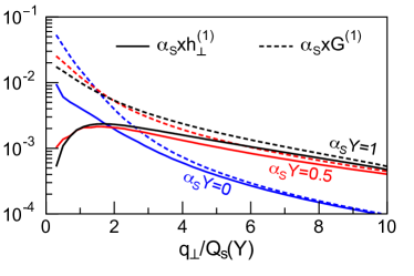
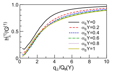
The functions $xG^{(1)}(x,q^{2}_{\perp})$ and $xh_{\perp}^{(1)}(x,q^{2}_{\perp})$ for the McLerran-Venugopalan (MV) model McLerran and Venugopalan (1994a, b) of a large nucleus were computed analytically in Refs. Metz and Zhou (2011); Dominguez et al. (2012). Explicit expressions for a more general theory of Gaussian fluctuations of the covariant gauge field $A^{+}$ were given in Ref. Dumitru and Skokov (2016); also see Refs. Marquet et al. (2016); Albacete et al. (2018). Numerical solutions of the JIMWLK evolution equations Balitsky (1996, 1998, 1999); Jalilian-Marian et al. (1997, 1999a, 1999b); Kovner and Milhano (2000); Kovner et al. (2000); Iancu et al. (2001a, b); Ferreiro et al. (2002); Weigert (2002) to small $x$ were presented in Refs. Dumitru et al. (2015); Marquet et al. (2016), shown in Fig. 1. At high transverse momentum one finds that $xh^{(1)}(x,q^{2}_{\perp})\to xG^{(1)}(x,q^{2}_{\perp})$ corresponding to maximal polarization. On the other hand, at low $q_{\perp}$ one has $xh^{(1)}(x,q^{2}_{\perp})/xG^{(1)}(x,q^{2}_{\perp})\ll 1$, implying that there the angular dependence of the cross-section (1, 2) is weak. For $q_{\perp}\sim Q_{s}(Y)$ these numerical solutions predict a substantial angular modulation of the dijet cross-section since $xh^{(1)}(x,q^{2}_{\perp})/xG^{(1)}(x,q^{2}_{\perp})\simeq 10\%-20\%$.

Our event generator described in the following Sec. III employs tabulated solutions of the leading order, fixed coupling JIMWLK evolution equations Balitsky (1996, 1998, 1999); Jalilian-Marian et al. (1997, 1999a, 1999b); Kovner and Milhano (2000); Kovner et al. (2000); Iancu et al. (2001a, b); Ferreiro et al. (2002); Weigert (2002) for $xh^{(1)}(Y,q^{2}_{\perp})$ and $xG^{(1)}(Y,q^{2}_{\perp})$, where $Y=\log x_{0}/x$. The initial condition at $x_{0}=0.01$ is given by the MV model. In particular, the initial MV saturation scale is set to $Q_{s}(x_{0})=1.2$ GeV corresponding to a large nucleus with $A\sim 200$ nucleons, on average over impact parameters.

II.1 Moments of inter-jet azimuthal angle

In this subsection we discuss the relation of $\langle\cos 2\phi\rangle$ introduced in the previous section to $\langle\cos 2\Phi\rangle$, where $\Phi$ is the azimuthal angle between the two jets (i.e. between $\vec{k}_{1\perp}$ and $\vec{k}_{2\perp}$). They are related through

$$\cos^{2}\Phi=\frac{(\vec{k}_{1\perp}\cdot\vec{k}_{2\perp})^{2}}{k_{1\perp}^{2}\,k_{2\perp}^{2}}~{}.$$ (9)

To obtain moments in the correlation limit at fixed $q_{\perp}$ and $P_{\perp}$ one inverts equations (3) to express $\vec{k}_{1\perp}=\vec{P}_{\perp}+z\vec{q}_{\perp}$ and $\vec{k}_{2\perp}=-\vec{P}_{\perp}+\bar{z}\vec{q}_{\perp}$, and performs an expansion of $\cos^{2}\Phi$ in powers of $q_{\perp}/P_{\perp}$. This leads to

$$\cos 2\Phi = 2\cos^{2}\Phi-1=1+\frac{q_{\perp}^{2}}{P_{\perp}^{2}}\left(\cos 2\phi-1\right)$$ (10)

$$+\frac{q_{\perp}^{4}}{P_{\perp}^{4}}\left[z\bar{z}-\left(1-2z\bar{z}\right)\cos 2\phi+\left(1-3z\bar{z}\right)\cos 4\phi\right]$$

$$+\cdots~{}.$$

We have dropped terms which vanish upon integration over $\phi$. The dots indicate contributions of higher order in $q_{\perp}/P_{\perp}$. Taking an average over $\phi$ at fixed $q_{\perp}$ and $P_{\perp}$ we obtain

$$\left<\cos 2\Phi\right>\bigr{|}_{q_{\perp},P_{\perp}} = 1+\frac{q_{\perp}^{2}}{P_{\perp}^{2}}\left<\cos 2\phi-1\right>$$ (11)

$$+\frac{q_{\perp}^{4}}{P_{\perp}^{4}}\left[z\bar{z}-\left(1-2z\bar{z}\right)\left<\cos 2\phi\right>+\left(1-3z\bar{z}\right)\left<\cos 4\phi\right>\right]$$

$$+\cdots~{}.$$

Since $d^{2}k_{1\perp}\,d^{2}k_{2\perp}\,\delta(q_{\perp}^{2}-(\vec{k}_{1\perp}+\vec{k}_{2\perp})^{2})\,\delta(P_{\perp}^{2}-(\bar{z}\vec{k}_{1\perp}-z\vec{k}_{2\perp})^{2})\sim d\phi$, the integral over $\phi$ is equivalent to an integral over $\vec{k}_{1\perp}$ and $\vec{k}_{2\perp}$ at fixed $q_{\perp}$ and $P_{\perp}$. On the r.h.s. of Eq. (11) one can now replace $\langle\cos 2\phi\rangle$ by $xh_{\perp}^{(1)}(x,q_{\perp})\,/\,xG^{(1)}(x,q_{\perp})$ times a prefactor, see Eq. (6). Note that this ratio of gluon distributions appears in $\left<\cos 2\Phi\right>$ with a suppression factor of $q_{\perp}^{2}/P_{\perp}^{2}$ whereas it contributes at ${\cal O}(1)$ to $\left<\cos 2\phi\right>$. Moreover, $xh_{\perp}^{(1)}(x,q_{\perp})\,/\,xG^{(1)}(x,q_{\perp})$ also contributes at order $q_{\perp}^{4}/P_{\perp}^{4}$ while power corrections to $\left<\cos 2\phi\right>$ only involve different correlators Dumitru and Skokov (2016).

II.2 Electron-proton/nucleus scattering

The cross-section for dijet production in electron-nucleus scattering is given by the product of the virtual photon fluxes of the electron with the $\gamma^{*}$-nucleus cross-sections discussed above Budnev et al. (1975); Drees and Zeppenfeld (1989); Nystrand (2005):

$$\frac{d\sigma^{e^{-}A\rightarrow q\bar{q}X}_{L,T}}{dQ^{2}dW^{2}d^{2}P_{\perp}d^{2}q_{\perp}dz}=f_{L,T}(Q^{2},W^{2})\,\frac{d\sigma^{\gamma_{L,T}^{\ast}A\rightarrow q\bar{q}X}}{d^{2}P_{\perp}d^{2}q_{\perp}dz}~{}.$$ (12)

Here,

$$\frac{d\sigma^{\gamma_{L,T}^{\ast}A\rightarrow q\bar{q}X}}{d^{2}P_{\perp}d^{2}q_{\perp}dz}=\int d^{2}b\int d\bar{z}\,E_{1}E_{2}\frac{d\sigma^{\gamma_{L,T}^{\ast}A\rightarrow q\bar{q}X}}{d^{3}k_{1}d^{3}k_{2}d^{2}b}~{}.$$ (13)

The of transversely and longitudinally polarized photon fluxes are given by

$$f_{T}(Q^{2},W^{2}) = \frac{\alpha_{\rm em}}{2\pi Q^{2}sy}\left(1+(1-y)^{2}\right)~{},$$ (14)

$$f_{L}(Q^{2},W^{2}) = \frac{\alpha_{\rm em}}{\pi Q^{2}sy}(1-y)~{},$$ (15)

with the inelasticity

$$y=\frac{W^{2}-M^{2}+Q^{2}}{s-M^{2}}~{}.$$ (16)

$M$ denotes the mass of the proton and $\sqrt{s}$ is the CM energy of the $e^{-}$ - proton collision. The $\gamma^{*}$-proton/nucleus cross-section on the r.h.s. of Eq. (12) depends on $W^{2}$ and $Q^{2}$ through Eq. (5). Note that Eqs. (14,15) do not apply in the limit $Q^{2}\to 0$ where the photon flux is effectively cut off at $Q^{2}_{\text{min}}\sim\xi^{2}m_{e}^{2}/(1-\xi)$ Budnev et al. (1975), with $m_{e}$ the mass of the electron and $\xi$ the momentum fraction of the photon relative to the electron. We are not concerned with $Q^{2}\,\,\vbox{\hbox{$\buildrel\displaystyle<\over{\sim}$}}\,\,1$ GeV² or $\xi\to 1$ here and hence ignore the modification of $f_{T,L}$ at low photon virtualities.

For given $W$ and $Q^{2}$, Bjorken-$x$ is defined as

$$x_{\text{Bj}}=\frac{Q^{2}}{W^{2}-M^{2}+Q^{2}}~{}.$$ (17)

III The event generator MCDijet

III.1 General description

The goal of the event generator MCDijet is to perform Monte-Carlo sampling of the dijet (quark and anti-quark) production cross-section described by Eq. (12). The code is open source and publicly available https://github.com/vskokov/McDijet (2018).

In what follows, we will often refer to the acceptance-rejection method (ACM) of generating random variables from a given probability distribution; although this method is fairly basic, it nevertheless proved sufficient for generating the required number of events on a single processor in a reasonable amount of time.

In order to make the MC generator computationally feasible we have adopted the following simplifying assumptions and approximations:

1. The dependence of the cross-section on the atomic number $A$ of the target enters via a single scale – the saturation momentum, $Q_{s0}\sim A^{1/6}$, at $x=x_{0}=0.01$. For a Au nucleus, averaged over impact parameters, we assume that $Q_{s0}=1.2$ GeV. This is compatible with $Q_{s0}\approx 0.44$ GeV for a proton target extracted in Refs. Albacete et al. (2009, 2011) from fits to HERA data. The current implementation is restricted to impact parameter averaged dijet production; realistic nuclear thickness functions and fluctuations of the nucleon configurations in the nucleus have not been implemented.

2. The Wilson lines in the field of the target at $x=x_{0}$ are sampled using the MV model. They are then evolved to $x<x_{0}$ using the fixed coupling Langevin form Blaizot et al. (2003); Rummukainen and Weigert (2004) of the JIMWLK renormalization group equation Balitsky (1996, 1998, 1999); Jalilian-Marian et al. (1997, 1999a, 1999b); Kovner and Milhano (2000); Kovner et al. (2000); Iancu et al. (2001a, b); Ferreiro et al. (2002); Weigert (2002), as described in Ref. Dumitru and Skokov (2015). Note that for many phenomenological applications running coupling corrections are known to be important; they are neglected in the current version of the event generator. Also, the JIMWLK evolution “time” $t=\alpha_{s}Y$ is converted to a momentum fraction $x/x_{0}=\exp(-t/\alpha_{s})$ using $\alpha_{s}=0.25$.

3. The Wilson lines are used to compute the dependence of $xG^{(1)}$ and $xh^{(1)}_{\perp}$ on the transverse momentum, $q_{\perp}$, and on $x$. The distributions are then averaged over the MV ensemble at the initial $x=x_{0}$, and over realizations of Langevin noise in small-$x$ evolution. The obtained averaged distributions are tabulated and stored in the file ”misc.dat” which will be used by the MCDijet generator. We therefore do not propagate configuration by configuration fluctuations into actual event-by-event fluctuations in quark anti-quark production.

MCDijet then performs the steps listed below:

• Using ACM based on the cross-section summed with respect to polarizations,

  $$\frac{d^{2}\sigma_{L,T}(Q^{2},W^{2})}{dQ^{2}dW^{2}}=f_{L,T}(Q^{2},W^{2})\int dP_{\perp}dq_{\perp}dzd\phi\frac{d\sigma_{L,T}}{dP_{\perp}dq_{\perp}dzd\phi}~{},$$ (18)

  where the integration is performed in a restricted range of $P_{\perp}$ and $q_{\perp}$ specified below, we sample $Q^{2}$ and $W^{2}$ in the ranges 4 GeV² $<Q^{2}<\frac{S-M^{2}}{1-x_{0}}x_{0}$ and $M^{2}+Q^{2}\left(\frac{1}{x_{0}}-1\right)<W^{2}<s$. The cross-sections $\frac{d\sigma_{L,T}}{dP_{\perp}dq_{\perp}dzd\phi}$ involve the WW distribution functions and thus implicitly depend on $x$, given in Eq. (5). Note that the calculation presented in this paper are based on the leading order expressions (1, 2). More realistic estimates of the absolute cross-section may require a multiplicative K-factor $K>1$. Here we provide a lower bound for the absolute cross-section and refrain from using a K-factor.

• The virtual photon may have either longitudinal or transverse polarization; it is assigned by sampling a random number $0<r<1$ uniformly. If

  $$r<\frac{\sigma_{L}(Q^{2},W^{2})}{\sigma_{L}(Q^{2},W^{2})+\sigma_{T}(Q^{2},W^{2})}$$

  the polarization is longitudinal; otherwise it is transverse.

• Using ACM and the differential cross-section for the photon polarization defined previously we generate a sample for $P_{\perp}$, $q_{\perp}$, $z$ and $\phi$.

• Using the obtained $P_{\perp}$, $q_{\perp}$, $\phi$ and $z$, we can compute the transverse components of the quark ($k_{1}$) and anti-quark ($k_{2}$) momenta

  $$\vec{k}_{1\perp} =P_{\perp}\vec{e}_{P}+zq_{\perp}\vec{e}_{q}\,,$$ (19)

  $$\vec{k}_{2\perp} =-P_{\perp}\vec{e}_{P}+\bar{z}q_{\perp}\vec{e}_{q}\,,$$ (20)

  where $\vec{e}_{P}=(\cos(\psi),\sin(\psi))$ and $\vec{e}_{q}=(\cos(\psi+\phi),\sin(\psi+\phi))$. Here, $\psi$ is sampled uniformly over $[0,2\pi[$.

• Finally, the longitudinal momenta are given by

  $$k_{1z} =\frac{1}{\sqrt{2}}zq^{+}-\frac{k_{1\perp}^{2}}{2\sqrt{2}zq^{+}},$$ (21)

  $$k_{2z} =\frac{1}{\sqrt{2}}\bar{z}q^{+}-\frac{k_{2\perp}^{2}}{2\sqrt{2}\bar{z}q^{+}},$$ (22)

  where

  $$q^{+} =\sqrt{2}\,y^{\prime}\,E_{e};\quad\quad y^{\prime}=\frac{1}{2}y\left(1+\sqrt{1+\left(\frac{2x_{\rm Bj}M}{Q}\right)^{2}}\right)~{},$$ (23)

  $$q^{-} =-\frac{Q^{2}}{2q^{+}}~{},$$ (24)

  and $x_{\rm Bj}$ and $y$ are defined in Eqs. (17) and (16) respectively. Here, $M$ denotes the mass of a proton, $E_{e}$ is the energy of the electron in the lab frame, and $q^{+}$ is the large light-cone component of the four-momentum $q^{\mu}$ of the virtual photon.

The sampled kinematic variables and the corresponding numerical value for the cross-section are then passed to Pythia. The interface between Pythia and MCDijet is described in Sec. IV.

The momentum assignments (19 - 24) define the specific frame in which we perform the analysis, see Fig. 2. That is, in this frame the transverse momenta of the virtual photon and of the target both vanish, the energy $E_{p}$ of the target nucleon(s) is equal to that in the lab frame, and the invariant $\gamma^{*}$ - nucleon collision energy squared is $W^{2}$. While, in principle, the analysis could be performed in any other longitudinally boosted frame, such as the Breit frame (see Appendix A) or the $\gamma^{*}$ - nucleon center of momentum frame, we have found that the reconstruction of the produced jets and of the target beam remnant is rather accurate in this “fixed $E_{p}$” frame; see Sec. IV for further details.

Figure 2: The reference frames:
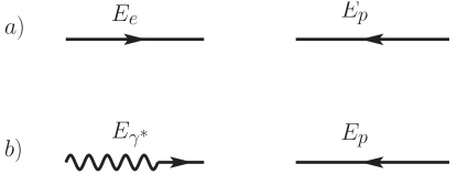
a) The laboratory frame. In the laboratory frame, the electron and the proton have zero transverse momenta; the energy of the electron (proton) is $E_{e}$ ($E_{p}$).
b) The analysis frame. Here, the virtual photon and the proton have zero transverse momenta; the energy of the proton is the same as in the laboratory frame, equal to $E_{p}$. The energy of the virtual photon is $E_{\gamma^{*}}=(q^{+}+q^{-})/\sqrt{2}$, see Eqs. (23) and (24).

III.2 Numerical results

Figure 3: Distributions of photon virtuality $Q$ and $\gamma^{*}$-nucleon c.m. collision energy $W$ for dijet events subject to the kinematic cuts described in the text.

In this subsection we show the distribution of dijet events over various kinematic variables. The target is assumed to be Au with $A=197$ nucleons, the $e^{-}-$Au collision energy is $\sqrt{s}=90$ GeV. The event selection cuts are $\surd Q^{2}>2$ GeV, $P_{\perp}>1.5\,q_{\perp}$, $q_{\perp}>1$ GeV, and $x$, $x_{\text{Bj}}<0.01$. The distributions of $Q$ and $W$ are shown in Fig. 3, those of photon polarizations and quark momentum fractions $z$ in Fig. 4.

Figure 4: Left: The contributions of transverse vs. longitudinal photon polarizations as functions of $Q$. Right: The distribution of the quark momentum fraction $z$.

IV Feasibility study for an Electron-Ion Collider

In this section, based on the theoretical foundation outlined above, we present a detailed study of the feasibility, requirements, and expected precision of measurements of the azimuthal anisotropy of dijets at a future Electron-Ion Collider (EIC). We find that, at an EIC Accardi et al. (2016), it is feasible to perform these measurement although high energies, $\sqrt{s}\sim 100$ GeV, large integrated luminosity of $\int L\mathrm{d}t\geq 20$ fb^-1, and excellent jet capabilities of the detector(s) will be required.

In order to verify the feasibility we have to show that (i) the anisotropy described by MCDijet (see Sec. III) is maintained in the reconstructed dijets measured in a realistic detector environment, that (ii) the DIS background processes can be suppressed sufficiently to not affect the level of anisotropy, and (iii) that $v_{2}^{L}$ and $v_{2}^{T}$ can be separated.

All studies presented here, were conducted with electron beams of 20 GeV and hadron beams with 100 GeV energy resulting in a center-of-mass energy of $\sqrt{s}=90$ GeV. As previously mentioned, our convention is that the electron (hadron) beam has positive (negative) longitudinal momentum. We use pseudo-data generated by the Monte Carlo generator MCDijet, PYTHIA 8.2 Sjöstrand et al. (2015) for showering of partons generated by MCDijet, and PYTHIA 6.4 Sjostrand et al. (2006) for background studies. Jets are reconstructed with the widely used FastJet package Cacciari et al. (2012).

IV.1 Azimuthal anisotropy of dijets

Figure 5: Kinematic range in $q_{\perp}$ vs. $P_{\perp}$ in the correlation limit, ${q_{\perp}}<{P_{\perp}}$, for two EIC energies, $\sqrt{s}$ = 40 and 90 GeV. On the left lines of constant $x$ for the respective energies are depicted while on the right we show lines of constant azimuthal anisotropy for longitudinally polarized virtual photons.

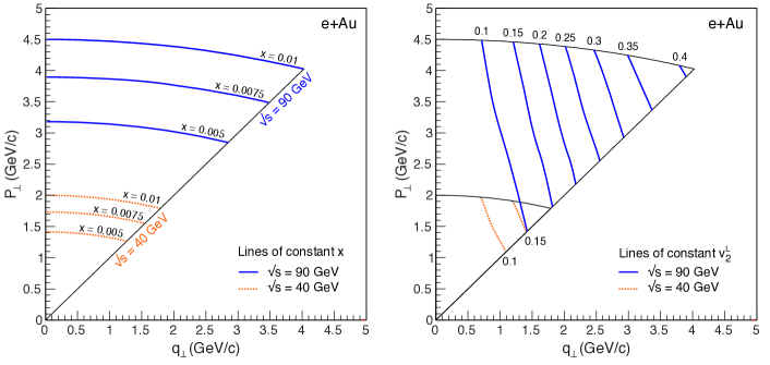
MCDijet generates a correlated pair of partons per event. It provides as output the 4-momenta of the two partons, the $z$ value, as well as general event characteristics such as $W$, $Q^{2}$, and $x$. Unless mentioned otherwise we restricted the generation of events to $4<Q^{2}<90$ GeV², $x,x_{\text{Bj}}<0.01$, $q_{\perp}>1$ GeV and $P_{\perp}>1.5q_{\perp}$. For the ion beam we use Au (A=197).

Figure 5 illustrates the kinematic range in $q_{\perp}$ versus $P_{\perp}$ on the parton level in the relevant region ${q_{\perp}}<{P_{\perp}}$, for two EIC energies, $\sqrt{s}$=40 and 90 GeV. In the left plot, we show lines of constant $x$ for both energies, and on the right, we depict lines of constant azimuthal anisotropy for longitudinally polarized virtual photons ($v_{2}^{L}$). It becomes immediately clear that substantial anisotropies, $v_{2}^{L}\geq 0.15$, can only be observed at the higher energy. Even more important, from an experimental point of view is the magnitude of the average transverse momentum $P_{\perp}$. Jet reconstruction requires sufficiently large jet energies to be viable. The lower the jet energy, the more particles in the jet cone fall below the typical particle tracking thresholds ($p_{T}\sim 250$ MeV/$c$ in our case), making jet reconstruction de facto impossible. For our studies, we therefore used the highest energy currently discussed for $e$+Au collisions at an EIC, $\sqrt{s}$ = 90 GeV.

The partons from MCDijet are subsequently passed to parton shower algorithms from the PYTHIA 8.2 event generator for jet generation. We assume the dipartons to be $u\bar{u}$ pairs. For jet finding we use the kt-algorithm from the FastJet package with a cone radius of $R=1$. In DIS events, jet finding is typically conducted in the Breit frame (see Sec. A) which is often seen as a natural choice to study the final state of a hard scattering. The Lorentz frame used in MCDijet is similar to the Breit frame in that the virtual photon and the proton have zero transverse momenta but distinguishes itself from the Breit frame by the incoming hadron (Au) beam having the same energy as in the laboratory frame. Jet finding studies in both frames showed no significant differences between the two. We therefore used the “analysis” frame described in Sec. III for all our studies.

Figure 6: $p_{T}$ and $\eta$ distributions of partons (filled circles) and reconstructed jets (filled squares) in the lab frame. The jet spectra are uncorrected.

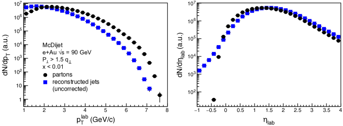
Fig. 6 shows the $p_{T}$ and $\eta$ distributions of partons (solid circles) from MCDijet and the corresponding reconstructed jets (solid squares) in the laboratory frame. The uncorrected jet spectra show the expected shift in $p_{T}$ due to the loss of particles below the chosen tracking threshold of 250 MeV/$c$. The pseudorapidity of the generated partons is well maintained by the jets with a typical r.m.s. of 0.4 units over the whole range. This is caused by unavoidable imperfections in the jet reconstruction. The smearing becomes more visible at $\eta<-0.5$ due to the steepness of the spectra.

Figure 7: Comparison of $q_{\perp}$ and $P_{\perp}$ distribution for partons (solid circles) and jets (solid squares).

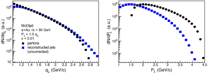
Fig. 7 shows the distribution of events over $q_{\perp}$ and $P_{\perp}$. One observes that at the level of reconstructed jets the distribution over $P_{\perp}$ is shifted by about $-0.5$ GeV, and slightly distorted. On the other hand, the distribution in $q_{\perp}$ of jets reproduces that of the underlying quarks rather accurately, except for the lowest ($q_{\perp}\sim 1$ GeV) and highest ($q_{\perp}\,\,\vbox{\hbox{$\buildrel\displaystyle>\over{\sim}$}}\,\,2.5$ GeV) transverse momentum imbalances. In a more in-depth analysis, which goes beyond the scope of this paper, the jet spectra would be corrected with sophisticated unfolding procedures (see for example Refs. Schmitt (2017); Biondi (2017)). Here, we simply correct the jet $P_{\perp}$ spectra by shifting it up so that $\langle P_{\perp}\rangle_{\mathrm{jet}}=\langle P_{\perp}\rangle_{\mathrm{parton}}$ for $P_{\perp}>1.5$ GeV/$c$. No corrections on $q_{\perp}$ were applied.

Figure 8: $\mathrm{d}\sigma/\mathrm{d}\phi$ distributions for parton pairs (blue points) generated with the MCDijet generator and corresponding reconstructed dijets (red points) in $\sqrt{s}$=90 GeV $e$+A collisions for $1.25<q_{\perp}<1.75$ GeV/$c$ and $3.00<P_{\perp}<3.50$ GeV/$c$. The error bars reflect an integrated luminosity of 10 fb^-1/A. The left plot shows the azimuthal anisotropy for all virtual photon polarizations while the middle and right plots correspond to transverse and longitudinal polarized photons, respectively. For details, see text.

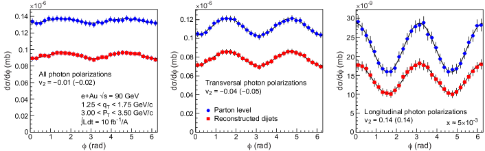
Figure 8 shows the resulting $\mathrm{d}\sigma/\mathrm{d}\phi$ distributions for the original parton pairs (blue solid points) and the reconstructed dijets (red solid squares) in $\sqrt{s}$=90 GeV $e$+Au collisions for $1.25<q_{\perp}<1.75$ GeV/$c$ and $3.00<P_{\perp}<3.50$ GeV/$c$. The results are based on 10M generated events but the error bars were scaled to reflect an integrated luminosity of 10 fb^-1/A. The left plot shows the azimuthal anisotropy for all virtual photon polarizations, and the middle and right plot for transversal and longitudinal polarized photons, respectively. The quantitative measure of the anisotropy, $v_{2}$, is listed in the figures. The values shown are those for parton pairs; the accompanying numbers in parenthesis denote the values derived from the reconstructed dijets. Note the characteristic phase shift of $\pi/2$ between the anisotropy for longitudinal versus transversally polarized photons. Despite this shift, the sum of both polarizations still adds up to nonzero net $v_{2}$ due to the dominance of transversely polarized photons, as depicted in the leftmost plot in Fig. 8.

The reconstructed dijets reflect the original anisotropy at the parton level remarkably well despite the dijet spectra not being fully corrected. The loss in dijet yield, mostly due to loss of low-$p_{T}$ particles, is on the order of $\sim 25$%. Since the key observable is the measured anisotropy, the loss in yield is of little relevance. However, when real data becomes available a careful study for possible biases will need to be carried out.

Figure 9: $\phi$, the angle between $\vec{P}_{\perp}$ and $\vec{q}_{\perp}$, as a function of the pseudorapidity, $\eta$, of each of the partons. The strong correlation indicates the sensitivity of the observed anisotropy in $\phi$ on the $\eta$ acceptance of potential experimental measurements.

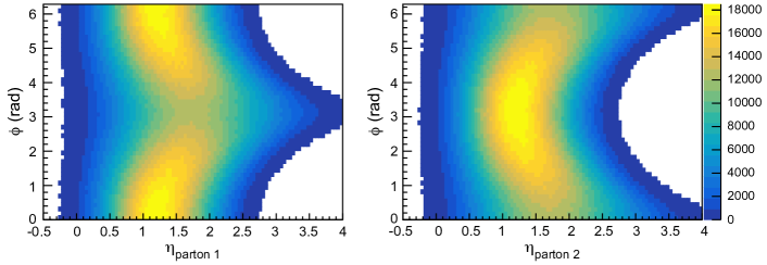
In our studies we noted the momentous correlation of the angle $\phi$ with the pseudorapidity, $\eta$, of the partons/jets illustrated in Fig. 9. This behavior is introduced through the $\eta$ dependence of $z$ and can be illustrated by expressing $z$ through the kinematics of the two partons as:

$$z=\frac{E_{1}+k_{1z}}{(E_{1}+k_{1z})+(E_{2}+k_{2z})}\,,$$ (25)

where $k_{iz}=E_{i}\tanh\eta_{i}=k_{i\perp}\sinh\eta_{i}$. Recall that $z$ is the momentum fraction of the first and $1-z$ that of the second parton/jet. Rewriting $P_{\perp}$ (see Eq. 3) as $\vec{P}_{\perp}=\vec{k}_{1\perp}-z\vec{q}_{\perp}$ shows that for $z\rightarrow 1$ large $P_{\perp}$ are biased towards $\vec{P}_{\perp}\uparrow\downarrow{\vec{q}_{\perp}}$ thus favoring $\phi\approx\pi$. On the other hand, writing $\vec{P}_{\perp}=-\vec{k}_{2\perp}+(1-z)\vec{q}_{\perp}$ we see that for $z\rightarrow 0$ large $|\vec{P}|$ prefers $\vec{P}_{\perp}\uparrow\uparrow\vec{q}_{\perp}$, i.e. $\phi\approx 0~{}\text{mod}~{}2\pi$. This has substantial impact on the experimental measurement since even in the absence of any anisotropy the finite $\eta$ acceptance of tracking detectors will generate a finite and positive $v_{2}$. On the other hand, a tight rapidity range also alters the actual anisotropy. For example the generated $v_{2}^{L}$ anisotropy in the right plot of Fig. 8 of 14% requires at a minimum a range of $0<\eta<3$; for $0<\eta<1.5$ the observed $v_{2}^{L}$ shrinks to $\sim 0.05$. This effect was verified with PYTHIA simulations where a limited acceptance showed a considerable effect despite PYTHIA having no mechanism to generate any intrinsic anisotropy. Only for wide acceptances with $\Delta\eta\geq 3$ does the $\phi$ distribution become flat. Measurements at an EIC will need to be corrected for these massive finite acceptance effects.

IV.2 Background studies

While MCDijet allows the study of the signal anisotropy in great detail it does neither generate complete events, nor does it allow us to derive the level of false identification of dijets in events unrelated to dijet production. The purity of the extracted signal sample ultimately determines if these measurements can be conducted. For studies of this kind we have to turn to PYTHIA6, an event generator that includes a relatively complete set of DIS processes.

Figure 10: Photon-gluon fusion processes that contributes to the 2+1 jet signal cross-section.

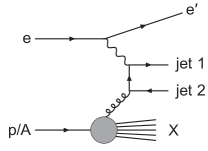
The presence of underlying event activity is key to answering the question if one can achieve a clear separation between the products of the hard partonic interaction and the beam remnants. For that reason, one usually labels an event as “2+1 jets” if it has 2 jets coming from the hard partonic interaction, with the “+1” indicating the beam remnants. The diagram in Fig. 10 thus depicts a 2+1-jet event.

While dijet studies have been successfully conducted in $e+p$ collisions at HERA (see for example Aktas et al. (2007); Gouzevitch (2008)) most such measurement have been carried out at high $Q^{2}$ and high jet energies ($E_{\mathrm{jet}}>10$ GeV). In our studies, however, we focus on moderately low virtualities and relatively small jet transverse momenta $P_{\perp}$ (see Fig. 6). Consequently, the dijet signal is easily contaminated by beam remnants. To minimize this background source we limit jet reconstruction to $1<\eta<2.5$, sufficiently far away from the beam fragmentation region.

Figure 11: $Q^{2}$ dependence of the signal-to-background ratio derived from PYTHIA6.

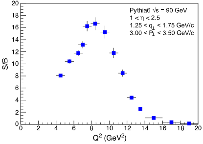
In our PYTHIA6 study we count $f_{i}+\gamma^{*}_{\mathrm{T,L}}\rightarrow f_{i}+g$ and $g+\gamma^{*}_{\mathrm{T,L}}\rightarrow f_{i}+\bar{f_{i}}$ (see Fig. 10) as signal and all other as background processes. By far the dominant background source is the standard LO DIS process $\gamma^{*}+q\rightarrow q$. Figure 11 illustrates the $Q^{2}$ dependence of the signal-to-background (S/B) ratio, i.e., the number of correctly reconstructed signal events over the number of events that were incorrectly flagged as containing a signal dijet process. The S/B ratio rises initially due to the improved dijet reconstruction efficiency towards larger $Q^{2}$ (or $P_{\perp}$) but then drops dramatically as particles from the beam remnant increasingly affect the jet finding. In what follows we therefore limit our study to $4\leq Q^{2}\leq 12$ GeV².

Figure 12: Azimuthal asymmetry in reconstructed dijet events from PYTHIA caused by the limited $\eta$ acceptance.

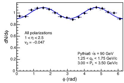
As discussed in Sec. IV.1, the necessity to limit dijet reconstruction to $\eta<2.5$ creates a substantial anisotropy illustrated in Fig. 12. The corresponding $v_{2}$ is always negative regardless of the polarization of the virtual photon and different from the true signal where $v_{2}^{L}$ and $v_{2}^{T}$ have opposite signs. This is a plain artifact of the limited pseudorapidity range. For a wider $\eta$ range the modulation vanishes but the S/B drops substantially since beam fragmentation remnants start to leak in. Since the anisotropy is of plain kinematic origin it can be easily derived from Monte-Carlo and corrected for. In the following we subtracted this $\eta$-range effect from our data sample.

Figure 13: $dN/d\phi$ distribution of signal and background jets after corrections.

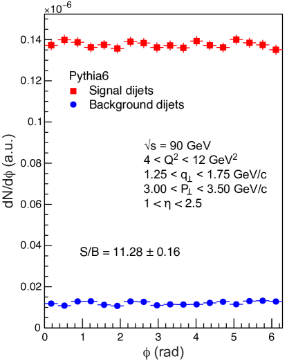
Figure 13 shows the resulting $dN/d\phi$ distributions for signal jets (solid squares) and background jets (solid circles). The signal-to-background ratio for the indicated cuts is S/B $\approx$ 11. After the finite $\eta$-range correction both, signal and background pairs show no modulation, as expected.

IV.3 Extracting $v_{2}^{L}$ and $v_{2}^{T}$

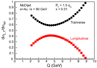
In order to derive the distribution of linearly polarized gluons via Eqs. (6), the contributions from transverse ($v_{2}^{T}$) and longitudinally polarized photons ($v_{2}^{L}$) need to be disentangled. With the exception of diffractive $J/\psi$ production, no processes in DIS exist where the polarization of the virtual photon can be measured directly. In our case there are 3 features that do make the separation possible: (i) $v_{2}^{L}$ and $v_{2}^{T}$ have opposite signs (see Fig. 8), (ii) the background contribution shows no anisotropy (see Fig. 13), and (iii) the relation

$$v_{2}^{\mathrm{unpol}}=\frac{Rv_{2}^{L}+v_{2}^{T}}{1+R}$$ (26)

ties together the unpolarized, i.e. measured, $v_{2}$ with the transverse and longitudinal components. $R$ is a kinematic factor depending entirely on known and measured quantities :

$$R=\frac{8\epsilon_{f}^{2}P_{\perp}^{2}\,z(1-z)}{(z^{2}+(1-z)^{2})\,(\epsilon_{f}^{4}+P_{\perp}^{4})}\,.$$ (27)

Figure 14: Result of a fit of combined signal and background to a data sample obtained in $\sqrt{s}=90$ GeV $e$+A collisions with an integrated luminosity of 10 fb^-1/A. For details see text.

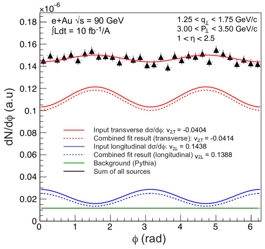
Our strategy is to perform a combined 5-parameter fit of all 3 components to the full data sample: The signal for longitudinal polarization ($\sigma_{L},v_{2}^{L}$), that for transverse polarization ($\sigma_{T},v_{2}^{T}$), and the flat background ($\sigma_{b}$). The fit uses the constraint provided by Eq. (27). We generated the data sample in a separate Monte-Carlo combining the signal from MCDijet with the background contribution from PYTHIA6 while smearing each data point randomly according to the statistics available at a given integrated luminosity. The fit provides the desired $v_{2}^{L}$ and $v_{2}^{T}$. In order to determine the corresponding errors we repeat the fit 10,000 times and derive the standard deviation from the obtained $dN/dv_{2}^{L,T}$ distributions. With reasonable accuracy the errors are distributed symmetrically about the true value.

Figure 14 shows the result of one typical fit on data generated for a integrated luminosity of 10 fb¹/A. The scatter and errors on the data points reflect the size of the potential data sample, the red and the blue curves illustrate the input (solid curve) and the fit result (dashed curve) for $v_{2}^{L}$ and $v_{2}^{T}$. The dashed curves were offset for better visibility.

Integrated Luminosity (fb-1/A)	$\delta v_{2}^{L}/v_{2}^{L}$ (%)	$\delta v_{2}^{T}/v_{2}^{T}(\%)$
1	23.7	16.7
10	7.5	5.3
20	5.5	3.9
50	3.4	2.4
100	2.4	1.6

Table 1: Relative error on the extracted $v_{2}^{L}$ and $v_{2}^{T}$ for various integrated luminosities.

Table 1 shows the derived relative errors on $v_{2}^{L}$ and $v_{2}^{T}$ for various integrated luminosities. These listed uncertainties refer only to the selected cuts of $1.25<q_{\perp}<1.75$ GeV/$c$, $3<P_{\perp}<3.5$ GeV/$c$, $4<Q^{2}<12$ GeV², and $1<\eta<2.5$. The errors show the expected $({\int{\cal{L}}\mathrm{d}t})^{-1/2}$ scaling. Systematic studies showed that the relative errors improve with increasing $P_{\perp}$, i.e., increasing $v_{2}$. Our results indicate that a proper measurement of the linearly polarized gluon distribution will require integrated luminosities of at least 20 fb^-1/A or more. Hence, this measurement would be a multi-year program assuming that an EIC initially starts off with luminosities around $10^{33}$ cm^-2 s^-1. The errors were derived assuming cross-section generated by MCDijet that are, as described earlier, somewhat lower than the ones from PYTHIA6.

V Outlook

Our current proof of principle analysis relied on a variety of simplifications and approximations as our main focus was on the reconstruction of relatively low $p_{T}$ jets and their angular distribution. In this section we address some improvements that would improve the accuracy of the model and of the analysis.

First off, a more realistic modelling of the impact parameter dependence of the thickness of the target nucleus would be useful. This is due to the fact that cuts on the minimal $P_{\perp}$ introduce a bias towards more central impact parameters as the dijet cross-section decreases with $P_{\perp}$ but increases with the saturation scale $Q_{s}$. In fact, this bias does also affect the shape of the small-$x$ gluon distributions as functions of $q_{\perp}/Q_{s}$ Dumitru and Skokov (2018, 2017); Dumitru et al. (2018). To account for this effect the event generator would have to employ individual JIMWLK field configurations rather than the unbiased average distributions.

Another improvement is to include running coupling corrections to the dijet cross-section and to small-$x$ JIMWLK evolution Lappi and Mäntysaari (2013). These would be important, in particular, if the analysis is performed over a broad range of transverse momenta.

The measurement of the distribution of linearly polarized gluons via the $\cos 2\phi$ azimuthal dependence requires significant jet momentum imbalance $q_{\perp}$ not much less than the saturation scale $Q_{s}$. On the other hand, the cross-section decreases steeply with $P_{\perp}$ and so, in practice, the ratio $q_{\perp}/P_{\perp}$ cannot be very small. Hence, power corrections to Eqs. (1, 2) may be significant and should be implemented. (Expressions for the leading power corrections in the large-$N_{c}$ limit can be found in Ref. Dumitru and Skokov (2016)).

One should also account for the Sudakov suppression which arises due to the presence of the two scales $q_{\perp}$ and $P_{\perp}$ Mueller et al. (2013); Zheng et al. (2014); Boer et al. (2017). In view of the relatively large ratio of $q_{\perp}/P_{\perp}$ employed in our analysis we do not expect a very large suppression of the amplitude of the $\cos 2\phi$ azimuthal dependence.

Given that the light-cone momentum fraction of the target partons is not very small even at the highest energies envisaged for an EIC it would be important to also account for the $\gamma^{*}+q\to g+q$ process, unless one attempts to identify events producing a gluon jet.

As the Electron-Ion Collider projects progresses detector concepts will become more refined. Once the design of the envisioned multi-purpose detector(s) are finalized the feasibility study discussed in this paper should be repeated using detailed detector effects (acceptance, resolution) and include full unfolding procedures that would improve over the simple corrections used in this work. There is an increasing interest in jet studies at an EIC that could potentially lead to improved jet finding procedures tailored to the specific kinematics and energies relevant for this study.

VI Summary and conclusions

This paper presents a study of the feasibility of measuring the conventional and linearly polarized Weizsäcker-Williams (WW) transverse momentum dependent (TMD) gluon distributions at a future high-energy electron-ion collider via dijet production in Deeply Inelastic Scattering on protons and nuclei at small $x$. In particular, we have found that suitable cuts in rapidity allow for a reliable separation of the dijet produced in the hard process from beam jet remnants. A cut on the photon virtuality, $Q^{2}\,\,\vbox{\hbox{$\buildrel\displaystyle<\over{\sim}$}}\,\,12$ GeV² suppresses the LO $\gamma^{*}q\to q+X$ process and leads to a signal to background ratio of order 10.

The jet transverse momentum $\vec{P}_{\perp}$ as well as the momentum imbalance $\vec{q}_{\perp}$, and the azimuthal angle $\phi$ between these vectors can all be reconstructed with reasonable accuracy even when $P_{\perp}$ is on the order of a few GeV. The $\phi$-averaged dijet cross-section determines the conventional WW TMD $xG^{(1)}(x,q^{2}_{\perp})$ while $v_{2}=\langle\cos 2\phi\rangle\sim xh^{(1)}_{\perp}(x,q^{2}_{\perp})\,/\,xG^{(1)}(x,q^{2}_{\perp})$ is proportional to the ratio of the linearly polarized to conventional WW TMDs. Furthermore, with known $P_{\perp}$, $Q^{2}$ and jet light cone momentum fraction $z$ it is possible to separate $v_{2}$ into the contributions from longitudinally or transversely polarized photons, respectively, to test the predicted sign flip, $v_{2}^{L}\cdot v_{2}^{T}<0$. We estimate that with an integrated luminosity of $20$ fb${}^{-1}/A$ one can determine $v_{2}^{L}$ and $v_{2}^{T}$ with a statistical error of approximately 5%.

Appendix A Breit frame

In any frame the ratio of plus momenta of quark and virtual photon is given by

$$z=\frac{k_{1}^{+}}{q^{+}}=\frac{|\vec{k}_{1}|+k_{1z}}{q_{0}+q_{z}}~{},$$ (28)

and therefore in any frame

$$k_{1z}=\frac{[z(E_{0}+q_{z})]^{2}-k_{1\perp}^{2}}{2z(q_{0}+q_{z})}~{}.$$ (29)

Similarly, for the antiquark

$$k_{2z}=\frac{[\bar{z}(E_{0}+q_{z})]^{2}-k_{2\perp}^{2}}{2\bar{z}(q_{0}+q_{z})}$$ (30)

In particular, in the Breit frame ($q_{0}=0$ and $|q_{z}|=Q$) we get

$$k_{1z}=\frac{(zQ)^{2}-k_{1\perp}^{2}}{2zq_{z}}\,.$$ (31)

Taking the longitudinal momentum of the photon to be positive (following the convention in the MCDijet code),

$$k_{1z}=\frac{(zQ)^{2}-k_{1\perp}^{2}}{2zQ}\,.$$ (32)

Recalling that $\bar{z}=1-z$ we can finally write the longitudinal momenta of the quark and anti-quark in the Breit frame in the form

$$k_{1z} = \frac{(zQ)^{2}-k_{1\perp}^{2}}{2zQ}$$ (33)

$$k_{2z} = \frac{[(1-z)Q]^{2}-k_{2\perp}^{2}}{2(1-z)Q}~{}.$$ (34)

The longitudinal boost leading from Eqs. (21,22) to these expressions defines the transformation from our “analysis frame” to the Breit frame.