The first tidal disruption flare in ZTF:
from photometric selection to multi-wavelength characterization
Abstract
We present Zwicky Transient Facility (ZTF) observations of the tidal disruption flare AT2018zr/PS18kh reported by Holoien et al. and detected during ZTF commissioning. The ZTF light curve of the tidal disruption event (TDE) samples the rise-to-peak exceptionally well, with 50 days of - and -band detections before the time of maximum light. We also present our multi-wavelength follow-up observations, including the detection of a thermal ( eV) X-ray source that is two orders of magnitude fainter than the contemporaneous optical/UV blackbody luminosity, and a stringent upper limit to the radio emission. We use observations of 128 known active galactic nuclei (AGN) to assess the quality of the ZTF astrometry, finding a median host-flare distance of 02 for genuine nuclear flares. Using ZTF observations of variability from known AGN and supernovae we show how these sources can be separated from TDEs. A combination of light-curve shape, color, and location in the host galaxy can be used to select a clean TDE sample from multi-band optical surveys such as ZTF or LSST.
1 Introduction
Stars that pass within the tidal radius of a supermassive black hole are disrupted and a sizable fraction of the resulting stellar debris gets accreted onto the black hole. When this disruption occurs outside the black hole event horizon (Hills, 1975), the result is a luminous flare of thermal emission (Rees, 1988). These stellar tidal disruption flares provide a unique tool to study black hole accretion and jet formation (e.g., Giannios & Metzger, 2011; van Velzen et al., 2011; Tchekhovskoy et al., 2014; Coughlin & Begelman, 2014; Piran et al., 2015; Pasham & van Velzen, 2018).
Optical transient surveys currently dominate the discovery of tidal disruption events (TDEs); about a dozen candidates have been found to date (for a recent compilation see van Velzen, 2018). All-sky X-ray surveys provide a second avenue for discovery (e.g., Saxton et al., 2017). By late 2019, the eROSITA mission (Merloni et al., 2012) should significantly increase the number of TDEs discovered via their X-ray emission (Khabibullin et al., 2014).
The observed blackbody radii of known TDEs (Gezari et al., 2009) suggest the soft X-ray photons of these flares originate from the inner part of a newly formed accretion disk ( cm), while the optical photons are produced at much larger radii, cm. Only a handful of optically selected TDEs have received sensitive X-ray follow-up observations within the first few months of discovery. So far, every case has been different; optically selected TDEs can be X-ray faint (Gezari et al., 2012), or have (Holoien et al., 2016b), or even show a decreasing optical-to-X-ray ratio (Gezari et al., 2017b).
Unification of the optical and X-ray properties of TDEs is possible if the optical emission is powered by shocks from intersecting stellar debris streams (Piran et al., 2015) and the X-ray photons are produced when parts of the stream get deflected toward a few gravitational radii and accreted (Shiokawa et al., 2015; Krolik et al., 2016). In this scenario, TDEs with low X-ray luminosities can be explained as inefficiencies in this circularization process. If instead most of the stellar debris is able to rapidly form an accretion disk (Bonnerot et al., 2016; Hayasaki et al., 2016), the X-rays from the disk have to be reprocessed at larger radii (e.g., Loeb & Ulmer, 1997; Bogdanović et al., 2004; Strubbe & Quataert, 2009; Guillochon et al., 2014) to yield the observed optical emission. When the reprocessing layer is optically thick to X-rays, TDE unification is established via orientation (e.g., Metzger & Stone, 2016; Auchettl et al., 2017; Dai et al., 2018).
Insight into the emission mechanism of TDEs can be gained from detailed observations of individual events. A lag of the X-ray emission in a cross-correlation analysis (Pasham et al., 2017) and a decrease of with time (Gezari et al., 2017a) have both been interpreted as evidence against a reprocessing scenario. However, these conclusions are not definitive since the X-ray diversity of TDEs has not yet been mapped out.
Clearly more TDEs with multi-wavelength observations are needed to make progress. As discussed in Hung et al. (2018), ZTF has the potential to significantly increase the TDE detection rate. Like the Palomar Transient Factory (PTF; Law et al., 2009; Rau et al., 2009), ZTF uses the Samuel Oschin 48" Schmidt telescope at Palomar Observatory. The biggest improvement over PTF is the 47 deg2 field-of-view of the ZTF camera (Bellm et al., 2019). The public Northern Sky Survey of ZTF (Graham et al., 2019) began on 2018 March 17, and covers the entire visible sky from Palomar in both the and bands every three nights (the Galactic Plane, , is covered with a one night cadence) to a typical depth of 20.5 mag. Using ZTF images, a stream of alerts (Patterson et al., 2019) containing transients and variable sources is generated by IPAC (Masci et al., 2019). Besides the essential photometric information, this stream contains value-added products such as the quality of the subtraction (Mahabal et al., 2019) and the probability that the alert is associated with a star versus a galaxy (Tachibana & Miller, 2018).
This paper is organized as follows. In Section 2 we present our observations of AT2018zr/PS18kh (Holoien et al., 2018), the first TDE with ZTF observations. This source was discovered in Pan-STARRS (Chambers et al., 2016) imaging data; both ATLAS (Tonry et al., 2018) and ASAS-SN (Shappee et al., 2014) also obtained detections, see Holoien et al. (2018). Here we present several new observations of this latest TDE: the ZTF light curve, XMM-Newton X-ray spectra, and VLA/AMI radio observations. The results from our HST campaign of UV spectroscopy and ground-based optical spectroscopic monitoring will be presented separately (T. Hung et al., in prep.). In Section 3 we compare AT2018zr to previous TDEs, supernovae (SNe), and AGN. In Section 4 we show the astrometric quality of ZTF data for nuclear transients. In Section 5 we discuss the results.
We adopt a flat cosmology with and . All magnitudes are reported in the AB system (Oke, 1974).
2 Observations
2.1 Selection of nuclear flares in ZTF data
During the commissioning phase of the ZTF camera and IPAC alerts pipeline we assessed the quality of the alert stream, focusing on nuclear transients. A transient was considered nuclear when it had at least one detection with a distance between the location of the source in the reference frame and the location of the transient that was smaller than 06. We also required a match within 1" of a known Pan-STARRS (Chambers et al., 2016) galaxy, selected using a star-galaxy score (Tachibana & Miller, 2018) of gcore . To remove sources with a very small flux increase, we also required that the point spread function (PSF) magnitude in the difference image (agpsf , see \citealt{Masci19}) and the PSF agnitude of the source in the reference image (agnr ) obey the relation: \verb agpsf agnr $<$ 1.5 ag.
To apply these filters and to obtain visual confirmation of the alerts we used the GROWTH Marshal (Kasliwal et al., 2019).
The objective of our commissioning effort was to understand the quality of the astrometry of nuclear transients; these results are presented in Section 4. We also obtained spectroscopic follow-up for a subset of nuclear transients, which led to the identification of the transient AT2018zr as a TDE candidate.
2.2 Brief history of AT2018zr
On 2018 March 3, the Pan-STARRS survey discovered transient PS18kh with an -band magnitude of , and registered it on the Transient Name Server (TNS111https://wis-tns.weizmann.ac.il) as AT2018zr the following day. On March 24, Tucker et al. (2018, ATel 11473) reported a potential TDE classification for this source based on multiple spectroscopic observations that showed a very blue continuum and some evidence for broad Balmer emission lines. Photometry from Pan-STARRS, ASASSN, and ATLAS, as well as further spectroscopic observations identifying AT2018zr as a TDE, are presented in Holoien et al. (2018).
On 2018 March 6, the source ZTF18aabtxvd222We internally nicknamed this source ZTF-NedStark. was identified as a nuclear transient by our ZTF alert pipeline. We obtained a spectroscopic follow-up observation using SEDM (Blagorodnova et al., 2018) on 2018, March 7, which showed a nearly featureless blue continuum. We triggered HST UV spectroscopic observations on 2018, March 27. We report these observations, plus our spectroscopic monitoring with several ground-based telescopes in Hung et al. 2018, in prep, from which we determine a redshift of .
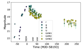
Upon further investigation we noticed the ZTF reference frame was contaminated with light from the transient, which prohibited an earlier detection; after rebuilding the reference images and applying an image subtraction algorithm (Zackay et al., 2016) that is similar to the one used in the IPAC pipeline, we found the first ZTF detection was on 2018 February 7 (Fig. 1).
2.3 Optical/UV observations of AT2018zr
Observations with the Neil Gehrels Swift Observatory (Swift; Gehrels et al., 2004) started on 2018 March 27 (PI: Holoien). We extracted the UVOT (Roming et al., 2005; Poole et al., 2008) flux with the help of the votsorce task, using an aperture radius of 5 arcsec.
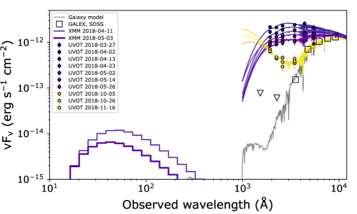
The flux of the host galaxy in the UVOT bands was estimated by fitting a synthetic galaxy spectrum (Conroy et al., 2009; Conroy & Gunn, 2010) to the SDSS model magnitudes (Stoughton et al., 2002; Ahn et al., 2014), see Table 1. To construct the synthetic galaxy spectrum we adopt the default assumptions for the stellar parameters: a Kroupa 2001 initial mass function with stellar masses ; Padova isochrones and MILES spectral library (Vazdekis et al., 2010). We assume an exponentially declining star formation rate (, with and as free parameters). We account for Galactic extinction by applying the Cardelli et al. (1989) extinction law with to the model spectrum. We also allow for extinction in the TDE host galaxy by modifying the model spectrum using a Calzetti et al. (2000) extinction law. The best-fit parameters for the formation history are Gyr and Gyr; the total stellar mass of the galaxy inferred for this model is .
Besides the Swift/UVOT and ZTF photometry, our light curve also includes P60/SEDM photometric data, host-subtracted using SDSS reference images (Fremling et al., 2016).
We correct the difference magnitude in each band for Galactic extinction, mag (Schlegel et al., 1998), again assuming a Cardelli et al. (1989) extinction law with . The resulting light curve is shown in Fig. 1 and the photometry is available in Table The first tidal disruption flare in ZTF: from photometric selection to multi-wavelength characterization.
By adding a blackbody spectrum to the synthetic host galaxy spectrum we find the best-fit temperature of the flare (Fig. 2). During the first 40 days of Swift monitoring the mean temperature was K, and appears constant with an rms of only K. Starting near May 11, 2018, until the last observation before the source moved out of the Swift visibility window (May 29, 2018), the temperature increased by a factor of (see also Holoien et al., 2018). The most recent observations, obtained when the source became visible again to Swift, show a large increase of the blackbody temperature; the UVOT observations are now on the Rayleigh Jeans tail of the SED and we obtain a lower limit to the temperature, K.
We searched for time lags between the optical and UV measurements taken with Swift using cross-correlations, following the procedure in Peterson et al. (1998). We first correct the light curves with a simple linear trend using a maximum-likelihood approach, and then use linear interpolation between data points in order to sample both UV and optical light curves on the same grid. We find no significant time lags between any combination of the the UV and optical bands at the 95% confidence level.
To search for outbursts in the years prior to the ZTF detection of AT2018zr, we applied a forced photometry method to the difference images from PTF and iPTF (Masci et al., 2017). We obtained 61 images, clustered at 6, 4, and 1 year before the current peak of the light curve. No prior variability was detected to a typical -band magnitude (5).
Using our ZTF observations of AT2018zr, we measure a mean angular distance between the host galaxy center and the flare of 012, or 162 pc. The rms of the offset, combining 46 offset measurements in Right Ascension and Declination and both - and -band detections, is 025. We thus conclude that the position of the flare is consistent with originating from the center of its host galaxy. Indeed, as we will see in Section 4, flares from AGN—which are expected to originate from the center of their galaxy—have a similar mean host-flare distance.
2.4 X-ray observations of AT2018zr
X-ray follow-up observations of AT2018zr were obtained using XMM-Newton (program 082204, PI: Gezari). Two epochs of XMM-Newton observations of the source were taken on 2018 April 11, and 2018 May 3 (see Table 2 for details). We reduced the XMM-Newton/pn data using the XMM-Newton Science Analysis System (SAS) and the newest calibration files. We started with the observation data files (ODFs) and followed standard procedures. Events were filtered with the conditions
ATTERN<= 4  and \verb FLAG==0 . We checked for high background flares (of which there were none). The source and background extraction regions are circular regions of radius 35". The response matrices were produced using {\sc rmfgen} and {\sc arfgen} in SAS. Spectral fitting was performed using
{\sc XS
EC v12.10 (Arnaud, 1996) with the c-statistic.
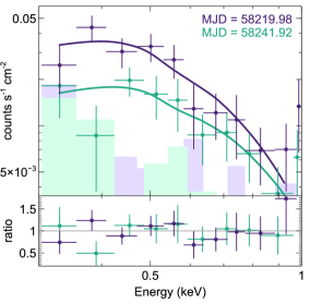
Both spectra are well described by a single blackbody component ( eV) and Galactic absorption ( cm-2; Kalberla et al. 2005). No additional absorption (at the redshift of the source) was required. The 0.3-1 keV luminosity of the first epoch is . The temperature of the thermal component remained constant between the two observations, though the flux decreased by a factor of 2. In Table 2 we list the full details of the spectral parameters.
The results from our XMM analysis are in mild conflict with the non-thermal spectrum (photon index ) reported by Holoien et al. (2018) using the Swift/XRT data. The XRT measurements overlap with our XMM-Newton epochs, but have a lower signal-to-noise ratio and less spectral coverage at low energies. Given these limitations, a thermal spectrum is easily mistaken for a steep power-law. Indeed, the XRT flux reported by Holoien et al. (2018) is consistent with the XMM-Newton flux. Given the superior quality of the XMM observations, we conclude that the thermal nature of the X-ray spectrum of AT2018zr is firmly established.
At late-time, days after peak, no XMM observations are available. To estimate the X-ray flux we binned the Swift/XRT observations of these epochs, yielding 14 photons in 77 ks of time on-source. The signal in this detection is not sufficient to measure the spectrum—although we note that the majority of the counts originate from the low-energy (0.3–1 keV) channels, indicating the spectrum has remained soft. To estimate the flux from the binned XRT observations we use a blackbody spectrum with a fixed temperature of 100 keV. We find that the late-time X-ray flux has not decreased significantly; the flux derived from the binned XRT observations is consistent with flux from the last XMM-Newton epoch; see Table 2.
2.5 Radio upper limits of AT2018zr
Radio observations of AT2018zr were obtained using the Arcminute Microkelvin Imager Large Array (AMI-LA; Zwart et al. 2008; Hickish et al. 2017) and the Karl G. Jansky Very Large Array (VLA; program 18A-373, PI: van Velzen). AMI observed on 2018 March 28, followed by the VLA on 2018 March 30 and April 28. The AMI data reduction was performed using the custom calibration pipeline reduce_dc (e.g. Perrott et al. 2013) with 3C 286 used as the primary calibrator, and J0745+3142 as the secondary calibrator. The same calibrators were used for both VLA observations. For the VLA data analysis, we made use of the NRAO pipeline products and flagged a few additional spectral channels after manual inspection for radio frequency interference. The calibrated visibilities were imaged using the Common Astronomy Software Application (CASA; McMullin et al., 2007) task clean, with natural weighting.
The source was not detected in any of our radio observations. The rms was determined from a source-free region adjacent to the target position. Our most sensitive observation was the first VLA epoch, which yields a 3 upper limit to the 10 GHz radio luminosity (defined as ) of erg s-1. Full details are listed in Table 3.
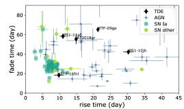
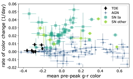
. Known TDEs have a longer rise and fade timescale compared to most SNe. Bottom: the mean - color versus its slope (Eq. 2) as measured during the first 100 days since the peak of the light curve. Unlike known SNe, all known TDEs have a near-constant color. Most AGN flares also have a constant color, but their mean colors (as measured in the difference image) show a much larger dispersion.
3 Comparison to known TDEs, SNe, and AGN flares
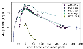
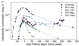
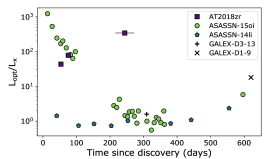
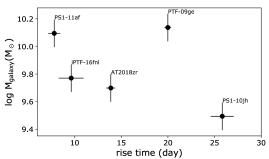
To date, only four333PTF-09djl and PTF-09axc (Arcavi et al., 2014) also have pre-peak detections, but no post-peak detections; ASASSN-18pg/AT2018dyb is reported (Brimacombe et al., 2018) to be detected on the rise, but its light curve has not been published yet. published optical TDEs have a resolved rise-to-peak: PS1-10jh (Gezari et al., 2012), PS1-11af (Chornock et al., 2014), PTF-09ge (Arcavi et al., 2014) and iPTF-16fnl (Blagorodnova et al., 2017). The earliest ZTF detection of AT2018zr is 50 days before the peak of the light curve. Measurements of the rise time to peak are important because this parameter is expected to scale with the mass of the black hole that disrupted the star (Rees, 1988; Lodato et al., 2009). In Fig. 4 we show the light curves of the five TDEs with pre-peak detections. We compare both the rest-frame -band luminosity and the blackbody luminosity. The -correction and bolometric correction were estimated using the mean blackbody temperature of the post-peak observations (van Velzen et al., 2018), except for AT2018zr, for which we used the temperature estimated from the nearest Swift/UVOT observation.
Our sample of nuclear flares from ZTF data is large enough to provide a meaningful comparison of the photometric properties of TDEs, SNe, and AGN flares. Selecting alerts that were discovered between May 1 and August 8, we obtain 840 sources. Of these, 331 can be classified as AGN using the Million quasar catalog (Flesch, 2015, v5.2.). Our sample contains 81 spectroscopically confirmed SNe (of which 62 are SNe Type Ia) and 3 cataclysmic variables (CVs). The spectroscopic observations for SN/CV classifications were obtained by the ZTF collaboration, with SEDM serving as the main instrument; SNe typing was established using SNID (Blondin & Tonry, 2007).
To be able to compare TDEs, SNe, CVs, and AGN flares, we use a single light-curve model to describe the observations of these transients. We compute the fading timescale of the light curve with respect to the rise time to the peak of the light curve using an exponential decay, while rise-to-peak is modeled using a Gaussian function:
| (1) |
This simplistic light-curve model is a compromise between using specific models for each type of object (e.g., SN Ia templates) and using a completely non-parametric approach (e.g., interpolating the light curve to measure the FWHM). Using all available ZTF data (i.e., including upper limits prior to the first detection of the alert), we fit both the -band and -band simultaneously. To model the SED, we use a constant color for the observation before the peak of the light curve, and a linear change of color with time for the post-peak observations:
| (2) |
The use of a constant color before the peak helps to get robust results from the fitting procedure (pre-peak light curves often contain too few points to constrain any color evolution), plus this light-curve model also matches the observed behavior of SN Ia, which only show significant cooling after maximum light (e.g., Hoeflich et al., 2017).
To summarize, our light-curve model has six free parameters: rise timescale (), fade timescale (), the time of peak (), flux at peak (), mean pre-peak color (), and rate of color change (, with units time-1).
For AT2018zr, we have no ZTF photometry post peak (because the flux of the transient is contained in the reference image of the public survey, which is not available for reprocessing until the first ZTF data release; Graham et al. 2019) and we instead use the Swift/UVOT photometry. For the other four TDEs with a resolved peak of the light curve, we include the published photometry444Obtained using the Open TDE Catalog, http://TDE.space. up to 100 days post-peak (when a longer temporal baseline is used, an exponential decay no longer provides a good description of the TDE light curve).
In Fig. 5 we show the result of applying our light-curve model to AT2018zr, other known TDEs, as well as the AGN, SNe and CVs in our sample of nuclear flares. We discuss these results in Section 5.4.
4 Host-flare astrometry in ZTF data
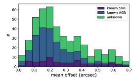
In the previous section we found that our sample of nuclear flares contains about 10% spectroscopically confirmed SNe. As explained in Section 2.1, the sample of nuclear flares was constructed from alerts with at least one detection with a host-flare distance smaller than 06. However we expect that the mean host-flare distance can be measured with a precision that is better than 06, thus facilitating a better separation of nuclear flares (AGN/TDEs) and SNe.
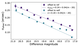
To understand how the measurement of the offset scales with the signal-to-noise ratio of the detection, we collected ZTF measurements for a sample of known AGN. To obtain a good measurement of the mean and rms of the offset, we required at least seven detections and a median host-flare distance , leaving 128 AGN. Under the assumption that the variability of these sources originates from the photometric center of their host galaxy, the observed rms of the offset yields the uncertainty, .
In Fig. 6 we show binned by the PSF magnitude of the flare in the difference image (). We find the following dependence between these two parameters
| (3) |
We can use this relation to compute the inverse-variance weighted mean of the offset. In Fig. 7 we show the weighted mean host-flare distance for the SNe, AGN, and unclassified flares in our nuclear flare sample (again using only sources with at least seven detections). Multiple observations of the same flare lead to an increased accuracy for the mean host-flare distance, yielding a typical uncertainty of 02 for nuclear flares with a few tens of detections (see the peak of the AGN distribution in Fig. 7).
The measurements of the host-flare offset are not independent because each measurement depends on the same reference frame to yield the position of the host. To show the astrometric accuracy without the contribution of the reference frame, we also report the rms of the offset with respect to the median position of the flare in the difference image (Fig. 6).
5 Discussion
5.1 Origin of the thermal emission mechanism
AT2018zr is the fifth optical/UV-selected TDE with an X-ray detection, and only the third source that was detected within a few months of its discovery. Close to peak, its optical-to-X-ray flux ratio is similar to that of ASASSN-15oi (Fig. 8). However, contrary to previous TDEs, AT2018zr shows an increase of ; its late-time X-ray luminosity remained approximately constant (Table 2), while the UV/optical blackbody luminosity increased.
The low X-ray luminosity of AT2018zr could be explained by a delay in the formation of the accretion disk, similar to the explanation proposed for the X-ray behavior of ASASSN-15oi (Gezari et al., 2017a). Yet, contrary to this TDE, the X-ray luminosity of AT2018zr remains weak compared to the optical/UV luminosity, suggesting no significant disk has formed yet. If instead disk formation is efficient and the optical emission is explained by reprocessing of emission from the inner disk, the low X-ray luminosity of AT2018zr must be explained by obscuration of this disk. However the increase of presents a challenge to this explanation. We generally expect that the optical depth for X-ray photons decreases with time because the processing layer expands/dilutes (e.g., Metzger & Stone, 2016) and this would yield a decrease of .
The blackbody radius corresponding to the single temperature model of the X-ray spectrum is cm for the first epoch of X-ray observations. This corresponds to the Schwarzschild radius () of a black hole with a mass of . Such a low-mass black hole is not expected given the properties of the host galaxy of AT2018zr. If half of the stellar mass of the galaxy is in the bulge, the predicted black hole mass (Gültekin et al., 2009) is (consistent with the black hole mass estimate of Holoien et al. 2018). If the observed X-ray photons originated from the inner part of an accretion disk, the intrinsic X-ray luminosity must be times higher to match the blackbody radius to the expected size of the inner disk. Part of this tension can be alleviated if the observed X-ray temperature is higher than the true temperature due to obscuration or a contribution of inverse Compton emission to the 0.3-1 keV spectrum. For example, if we adopt the upper limit to the intrinsic absorption from the X-ray spectral fit of , then the inferred blackbody temperature decreases by a factor of 2 and the unabsorbed X-ray luminosity increases by a factor of 1800, yielding a blackbody radius that is a factor of 170 larger and of the same of order as the expected size of the inner disk.
We thus conclude that if a modest amount of neutral gas has affected the intrinsic X-ray spectrum, we can explain the unexpectedly small radius of the X-ray photosphere inferred from the observed spectrum. Based on the increase of , we suggest this obscuring material would be outside the optical photosphere, i.e., the absorbed X-ray energy is not the source of the observed optical/UV emission of AT2018zr.
Even after accounting for the potential effect of absorption on the X-ray spectrum, the X-ray blackbody radius from our XMM-Newton observations is two orders of magnitude smaller than the inner radius of of the elliptical disk model proposed by Holoien et al. (2018). While this extended elliptical disk could explain the properties of the optical emission lines, our X-ray observations suggest a small, compact accretion disk is present as well.
Based on Swift/UVOT observations that covered the first three months after peak, Holoien et al. (2018) reported a modest (40%) increase in the optical/UV blackbody temperature. After a gap in the Swift coverage (due to Sun constraints), we find that the temperature has increased by at least a factor of 3; K in the latest Swift observations, obtained 250 days after peak. The result of this temperature evolution is an flattening of the UV light curve (Fig. 1) and an increase of the blackbody luminosity (Fig. 4). The UV/optical blackbody radius has decreased by an order of magnitude: from cm for the observations near peak to cm. We note that the Swift UV observations near peak show a hint of a blue excess (Fig. 2). This suggests the hot component detected at late-time was also present at early-time and became more prominent due to the fading of the lower-temperature component.
The observed flattening of the UV light curve of AT2018zr (Fig. 1) is a common feature of TDEs and can be interpreted as an increased contribution of an accretion disk to the SED (van Velzen et al., 2018). The current blackbody temperature of AT2018zr (about 250 days post-peak) is also similar to the temperature of most TDEs that have been detected at UV wavelengths 1–10 years after peak (van Velzen et al., 2018). However, the factor 4 increase of the blackbody temperature of AT2018zr is uncommon (cf. Hung et al., 2017, their Fig. 11). The light curve of the TDE ASASSN-15oi (Holoien et al., 2016a) showed a temperature increase of a factor (and a factor of decrease of the blackbody radius) during the first 100 days of observations. We note that the early-time optical/UV temperature of AT2018zr ( K) was relatively low, which could explain why the temperature increase is larger compared to most previous TDES. The TDE PTF-09ge also displayed a relatively low temperature near peak (as measured from the - color), followed by a factor of 4 increase to the blackbody temperature inferred from HST observations obtained 6 years after peak (van Velzen et al., 2018).
5.2 Interpretation of radio non-detection
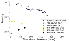
The upper limit to the radio luminosity of AT2018zr is one order of magnitude lower than the observed radio emission of the TDE ASASSN-14li (van Velzen et al., 2016a; Alexander et al., 2016; Bright et al., 2018). Currently, only the TDE iPTF-16fnl (Blagorodnova et al., 2017) has received radio follow-up observations close to the peak of the flare with a similar sensitivity. This source was also not detected at radio frequencies. However, this flare was exceptional, being the faintest and fastest fading TDE to date (see Fig. 4). The optical properties of AT2018zr, on the other hand, are similar to the mean properties of the current TDE sample (see Figs. 4 & 5 and Hung et al. 2017).
Our radio non-detection rules out the hypothesis that TDEs with a typical optical luminosity and fade timescale produce radio emission similar to that of ASASSN-14li (Fig. 9). However, the X-ray luminosity of AT2018zr is two orders of magnitude lower than ASASSN-14li (Holoien et al., 2016b). If the radio luminosity scales linearly with the power of the accretion disk, as observed for ensembles of radio-loud quasars (Rawlings & Saunders, 1991; Falcke et al., 1999; van Velzen et al., 2015) and for ASASSN-14li (Pasham & van Velzen, 2018), the expected radio flux of AT2018zr would be too faint to be detectable.
Free–free absorption is unlikely to affect the 10 GHz flux of AT2018zr because it would require an unrealistically high electron density. For an electron temperature of K, we require an emission measure (EM) of at least pc cm-6 to yield a significant optical depth () for free-free absorption at 10 GHz (e.g., Condon, 1992). This limit on the EM corresponds to a mean electron density of cm-3 within one parsec, which is at least two orders of magnitude larger than the particle density within the central parsec of our Galactic Center (Baganoff et al., 2003; Quataert, 2004) or the circumnuclear density inferred from the jetted TDEs (Berger et al., 2012; Generozov et al., 2017; Eftekhari et al., 2018). For higher electron temperatures, as expected for galaxy centers (Lazio et al., 1999), the lower limit on the EM would increase even further.
5.3 Rise timescale and Black Hole Mass
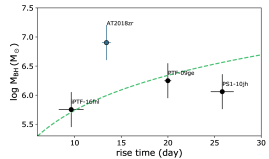
While our current sample of TDEs with a resolved rise-to-peak is still small, we can start to search for the anticipated correlation between black hole mass and rise timescale (Rees, 1988; Lodato et al., 2009). To estimate the black hole mass we use the velocity dispersion measurements from Wevers et al. (2017) and the Gültekin et al. (2009) - relation. For the host galaxy of AT2018zr, a velocity dispersion measurement is not yet available and we adopt the black hole mass from the bulge mass (, see Section 5.1). To provide a more uniform comparison we also consider the relation between rise time and total stellar mass. The results are shown in Fig. 10.
Our measurement of the rise time uses a Gaussian function (Eq.1), which has no defined start time. To be able to compare our measurement to the predicted fallback timescale () we assume the disruption happened at (i.e., when the flux in the model light curve is just 1% of the flux at peak). In Fig. 10 we show the predicted rise time from the theoretical fallback time of Stone et al. (2013), for the disruption of a star with a mass of 1 and an impact parameter of unity,
| (4) |
We find no correlation between the rise time and total galaxy mass. This could be considered surprising given that a correlation between the fade timescale and the black hole mass has been reported (Blagorodnova et al., 2017; Wevers et al., 2017). However, our results also show that the rise and fade timescales themselves appear to be uncorrelated (Fig. 5). It could be possible that the post-peak light curve provides a better tracer for the fallback rate—and thus a better mass estimate (Mockler et al., 2018)—compared to the rise-to-peak.
5.4 Photometric selection of TDEs in optical surveys
Using only 3 months of ZTF data, we confirm the conclusions from earlier TDE population studies (Gezari et al., 2009; van Velzen et al., 2011; Holoien et al., 2016a; Hung et al., 2017), showing that TDEs are a class of flares with a shared set of photometric properties.
Our work is the first to quantify the distribution of rise and fade timescales of TDEs. We find that most TDEs have both a longer rise time and fade time compared to SNe (Fig. 5, top panel). The TDE iPTF-16fnl is an interesting exception, displaying a rise timescale at the edge of the SN Ia distribution and a fade timescale that is faster compared to most SNe.
Using only pre-peak observations, effective removal of SNe Ia is possible by restricting to flares with a rise time (, Eq. 1) that is longer than days. While AGN flares can have a wide range of rise/fade timescales, very few rise and fade within a few months. Only 5% of AGN in our sample of nuclear flares have rise and fade timescales that fall within the range spanned by known TDEs.
The largest contrast between TDEs and SNe is found when we consider the mean color and color change (Fig. 5). We see that TDEs cluster in the region of blue and constant colors (van Velzen et al., 2011). Near their peak, some SNe can be as blue as TDEs, yet these SNe also cool very fast.
In this work we have demonstrated how several photometric properties can be used to separate TDEs from AGN flares and SNe: the rise/fade timescale (Fig. 5, top panel), the flare’s color and its evolution (Fig. 5, bottom panel), and the location of the flare in the host galaxy (Fig. 7). Additional selection on the host galaxy properties can be used to further reduce AGN contamination (e.g., prior variability, the amplitude of the flux increase). While each of these metrics has exceptions (e.g., TDE from faint galaxies have large astrometric uncertainties on the host-flare offset, and some TDE rise and fade rapidly), photometric selection will be unavoidable in the era of the Large Synoptic Survey Telescope (LSST). The TDEs detected by LSST will be too faint and too numerous ( per year; van Velzen et al., 2011) to use spectroscopic follow-up observations for classification.
References
- Ahn et al. (2014) Ahn, C. P., Alexandroff, R., Allende Prieto, C., et al. 2014, ApJS, 211, 17
- Alexander et al. (2016) Alexander, K. D., Berger, E., Guillochon, J., Zauderer, B. A., & Williams, P. K. G. 2016, ApJ, 819, L25
- Arcavi et al. (2014) Arcavi, I., Gal-Yam, A., Sullivan, M., et al. 2014, ApJ, 793, 38
- Arnaud (1996) Arnaud, K. A. 1996, in Astronomical Society of the Pacific Conference Series, Vol. 101, Astronomical Data Analysis Software and Systems V, ed. G. H. Jacoby & J. Barnes, 17
- Astropy Collaboration et al. (2018) Astropy Collaboration, Price-Whelan, A. M., Sipócz, B. M., et al. 2018, AJ, 156, 123
- Auchettl et al. (2017) Auchettl, K., Guillochon, J., & Ramirez-Ruiz, E. 2017, ApJ, 838, 149
- Baganoff et al. (2003) Baganoff, F. K., Maeda, Y., Morris, M., et al. 2003, ApJ, 591, 891
- Bellm et al. (2019) Bellm, E. C., Kulkarni, S. R., Graham, M. J., et al. 2019, PASP, 131, 018002
- Berger et al. (2012) Berger, E., Zauderer, A., Pooley, G. G., et al. 2012, ApJ, 748, 36
- Blagorodnova et al. (2017) Blagorodnova, N., Gezari, S., Hung, T., et al. 2017, ApJ, 844, 46
- Blagorodnova et al. (2018) Blagorodnova, N., Neill, J. D., Walters, R., et al. 2018, PASP, 130, 035003
- Blondin & Tonry (2007) Blondin, S., & Tonry, J. L. 2007, ApJ, 666, 1024
- Bogdanović et al. (2004) Bogdanović, T., Eracleous, M., Mahadevan, S., Sigurdsson, S., & Laguna, P. 2004, ApJ, 610, 707
- Bonnerot et al. (2016) Bonnerot, C., Rossi, E. M., Lodato, G., & Price, D. J. 2016, MNRAS, 455, 2253
- Bright et al. (2018) Bright, J. S., Fender, R. P., Motta, S. E., et al. 2018, MNRAS, 475, 4011
- Brimacombe et al. (2018) Brimacombe, J., Cornect, R., & Stanek, K. Z. 2018, Transient Name Server Discovery Report, 982
- Calzetti et al. (2000) Calzetti, D., Armus, L., Bohlin, R. C., et al. 2000, ApJ, 533, 682
- Cardelli et al. (1989) Cardelli, J. A., Clayton, G. C., & Mathis, J. S. 1989, ApJ, 345, 245
- Chambers et al. (2016) Chambers, K. C., Magnier, E. A., Metcalfe, N., et al. 2016, ArXiv e-prints, arXiv:1612.05560
- Chornock et al. (2014) Chornock, R., Berger, E., Gezari, S., et al. 2014, ApJ, 780, 44
- Condon (1992) Condon, J. J. 1992, ARA&A, 30, 575
- Conroy & Gunn (2010) Conroy, C., & Gunn, J. E. 2010, ApJ, 712, 833
- Conroy et al. (2009) Conroy, C., Gunn, J. E., & White, M. 2009, ApJ, 699, 486
- Coughlin & Begelman (2014) Coughlin, E. R., & Begelman, M. C. 2014, ApJ, 781, 82
- Dai et al. (2018) Dai, L., McKinney, J. C., Roth, N., Ramirez-Ruiz, E., & Miller, M. C. 2018, ApJ, 859, L20
- Eftekhari et al. (2018) Eftekhari, T., Berger, E., Zauderer, B. A., Margutti, R., & Alexander, K. D. 2018, ApJ, 854, 86
- Falcke et al. (1999) Falcke, H., Bower, G. C., Lobanov, A. P., et al. 1999, ApJ, 514, L17
- Flesch (2015) Flesch, E. W. 2015, PASA, 32, e010
- Fremling et al. (2016) Fremling, C., Sollerman, J., Taddia, F., et al. 2016, A&A, 593, A68
- Gabriel et al. (2004) Gabriel, C., Denby, M., Fyfe, D. J., et al. 2004, in Astronomical Society of the Pacific Conference Series, Vol. 314, Astronomical Data Analysis Software and Systems (ADASS) XIII, ed. F. Ochsenbein, M. G. Allen, & D. Egret, 759
- Gehrels et al. (2004) Gehrels, N., Chincarini, G., Giommi, P., et al. 2004, ApJ, 611, 1005
- Generozov et al. (2017) Generozov, A., Mimica, P., Metzger, B. D., et al. 2017, MNRAS, 464, 2481
- Gezari et al. (2017a) Gezari, S., Cenko, S. B., & Arcavi, I. 2017a, ApJ, 851, L47
- Gezari et al. (2009) Gezari, S., Heckman, T., Cenko, S. B., et al. 2009, ApJ, 698, 1367
- Gezari et al. (2012) Gezari, S., Chornock, R., Rest, A., et al. 2012, Nature, 485, 217
- Gezari et al. (2017b) Gezari, S., Hung, T., Cenko, S. B., et al. 2017b, ApJ, 835, 144
- Giannios & Metzger (2011) Giannios, D., & Metzger, B. D. 2011, MNRAS, 416, 2102
- Graham et al. (2019) Graham, M. J., Kulkarni, S. R., Bellm, E. C., et al. 2019, PASP in press, arXiv:1902.01945
- Guillochon et al. (2014) Guillochon, J., Manukian, H., & Ramirez-Ruiz, E. 2014, ApJ, 783, 23
- Gültekin et al. (2009) Gültekin, K., Richstone, D. O., Gebhardt, K., et al. 2009, ApJ, 698, 198
- Hayasaki et al. (2016) Hayasaki, K., Stone, N., & Loeb, A. 2016, MNRAS, 461, 3760
- Hickish et al. (2017) Hickish, J., Razavi-Ghods, N., Perrott, Y. C., et al. 2017, ArXiv e-prints, arXiv:1707.04237
- Hills (1975) Hills, J. G. 1975, Nature, 254, 295
- Hoeflich et al. (2017) Hoeflich, P., Hsiao, E. Y., Ashall, C., et al. 2017, ApJ, 846, 58
- Holoien et al. (2016a) Holoien, T. W.-S., Kochanek, C. S., Prieto, J. L., et al. 2016a, MNRAS, 463, 3813
- Holoien et al. (2016b) —. 2016b, MNRAS, 455, 2918
- Holoien et al. (2018) Holoien, T. W.-S., Huber, M. E., Shappee, B. J., et al. 2018, ArXiv e-prints, arXiv:1808.02890
- Hung et al. (2017) Hung, T., Gezari, S., Blagorodnova, N., et al. 2017, ApJ, 842, 29
- Hung et al. (2018) Hung, T., Gezari, S., Cenko, S. B., et al. 2018, The Astrophysical Journal Supplement Series, 238, 15
- Kalberla et al. (2005) Kalberla, P. M. W., Burton, W. B., Hartmann, D., et al. 2005, A&A, 440, 775
- Kasliwal et al. (2019) Kasliwal, M. M., Cannella, C., Bagdasaryan, A., et al. 2019, PASP in press, arXiv:1902.01934
- Khabibullin et al. (2014) Khabibullin, I., Sazonov, S., & Sunyaev, R. 2014, MNRAS, 437, 327
- Krolik et al. (2016) Krolik, J., Piran, T., Svirski, G., & Cheng, R. M. 2016, ApJ, 827, 127
- Kroupa (2001) Kroupa, P. 2001, MNRAS, 322, 231
- Law et al. (2009) Law, N. M., Kulkarni, S. R., Dekany, R. G., et al. 2009, PASP, 121, 1395
- Lazio et al. (1999) Lazio, T. J. W., Cordes, J. M., Anantharamaiah, K. R., Goss, W. M., & Kassim, N. E. 1999, in Astronomical Society of the Pacific Conference Series, Vol. 186, The Central Parsecs of the Galaxy, ed. H. Falcke, A. Cotera, W. J. Duschl, F. Melia, & M. J. Rieke, 441
- Lodato et al. (2009) Lodato, G., King, A. R., & Pringle, J. E. 2009, MNRAS, 392, 332
- Loeb & Ulmer (1997) Loeb, A., & Ulmer, A. 1997, ApJ, 489, 573
- Mahabal et al. (2019) Mahabal, A., Rebbapragada, U., Walters, R., et al. 2019, PASP, 131, 038002
- Masci et al. (2017) Masci, F. J., Laher, R. R., Rebbapragada, U. D., et al. 2017, PASP, 129, 014002
- Masci et al. (2019) Masci, F. J., Laher, R. R., Rusholme, B., et al. 2019, PASP, 131, 018003
- McMullin et al. (2007) McMullin, J. P., Waters, B., Schiebel, D., Young, W., & Golap, K. 2007, in Astronomical Society of the Pacific Conference Series, Vol. 376, Astronomical Data Analysis Software and Systems XVI, ed. R. A. Shaw, F. Hill, & D. J. Bell, 127
- Merloni et al. (2012) Merloni, A., Predehl, P., Becker, W., et al. 2012, ArXiv e-prints, arXiv:1209.3114
- Metzger & Stone (2016) Metzger, B. D., & Stone, N. C. 2016, MNRAS, 461, 948
- Mockler et al. (2018) Mockler, B., Guillochon, J., & Ramirez-Ruiz, E. 2018, ApJ in press, arXiv:1801.08221
- Oke (1974) Oke, J. B. 1974, ApJS, 27, 21
- Pasham et al. (2017) Pasham, D. R., Cenko, S. B., Sadowski, A., et al. 2017, ApJ, 837, L30
- Pasham & van Velzen (2018) Pasham, D. R., & van Velzen, S. 2018, ApJ, 856, 14
- Patterson et al. (2019) Patterson, M. T., Bellm, E. C., Rusholme, B., et al. 2019, PASP, 131, 018001
- Perrott et al. (2013) Perrott, Y. C., Scaife, A. M. M., Green, D. A., et al. 2013, MNRAS, 429, 3330
- Peterson et al. (1998) Peterson, B. M., Wanders, I., Horne, K., et al. 1998, PASP, 110, 660
- Piran et al. (2015) Piran, T., Svirski, G., Krolik, J., Cheng, R. M., & Shiokawa, H. 2015, ApJ, 806, 164
- Poole et al. (2008) Poole, T. S., Breeveld, A. A., Page, M. J., et al. 2008, MNRAS, 383, 627
- Quataert (2004) Quataert, E. 2004, ApJ, 613, 322
- Rau et al. (2009) Rau, A., Kulkarni, S. R., Law, N. M., et al. 2009, PASP, 121, 1334
- Rawlings & Saunders (1991) Rawlings, S., & Saunders, R. 1991, Nature, 349, 138
- Rees (1988) Rees, M. J. 1988, Nature, 333, 523
- Roming et al. (2005) Roming, P. W. A., Kennedy, T. E., Mason, K. O., et al. 2005, Space Sci. Rev., 120, 95
- Saxton et al. (2017) Saxton, R. D., Read, A. M., Komossa, S., et al. 2017, A&A, 598, A29
- Schlegel et al. (1998) Schlegel, D. J., Finkbeiner, D. P., & Davis, M. 1998, ApJ, 500, 525
- Shappee et al. (2014) Shappee, B. J., Prieto, J. L., Grupe, D., et al. 2014, ApJ, 788, 48
- Shiokawa et al. (2015) Shiokawa, H., Krolik, J. H., Cheng, R. M., Piran, T., & Noble, S. C. 2015, ApJ, 804, 85
- Stone et al. (2013) Stone, N., Sari, R., & Loeb, A. 2013, MNRAS, 435, 1809
- Stoughton et al. (2002) Stoughton, C., Lupton, R. H., Bernardi, M., et al. 2002, AJ, 123, 485
- Strubbe & Quataert (2009) Strubbe, L. E., & Quataert, E. 2009, MNRAS, 400, 2070
- Tachibana & Miller (2018) Tachibana, Y., & Miller, A. A. 2018, PASP, 130, 128001
- Tchekhovskoy et al. (2014) Tchekhovskoy, A., Metzger, B. D., Giannios, D., & Kelley, L. Z. 2014, MNRAS, 437, 2744
- Tonry et al. (2018) Tonry, J. L., Denneau, L., Heinze, A. N., et al. 2018, PASP, 130, 064505
- Tucker et al. (2018) Tucker, M. A., Huber, M., Shappee, B. J., et al. 2018, The Astronomer’s Telegram, 11473
- van Velzen (2018) van Velzen, S. 2018, ApJ, 852, 72
- van Velzen et al. (2015) van Velzen, S., Falcke, H., & Körding, E. 2015, MNRAS, 446, 2985
- van Velzen et al. (2013) van Velzen, S., Frail, D. A., Körding, E., & Falcke, H. 2013, A&A, 552, A5
- van Velzen et al. (2011) van Velzen, S., Körding, E., & Falcke, H. 2011, MNRAS, 417, L51
- van Velzen et al. (2016a) van Velzen, S., Mendez, A. J., Krolik, J. H., & Gorjian, V. 2016a, ApJ, 829, 19
- van Velzen et al. (2018) van Velzen, S., Stone, N. C., Metzger, B. D., et al. 2018, ArXiv e-prints, arXiv:1809.00003
- van Velzen et al. (2011) van Velzen, S., Farrar, G. R., Gezari, S., et al. 2011, ApJ, 741, 73
- van Velzen et al. (2016b) van Velzen, S., Anderson, G. E., Stone, N. C., et al. 2016b, Science, 351, 62
- Vazdekis et al. (2010) Vazdekis, A., Sánchez-Blázquez, P., Falcón-Barroso, J., et al. 2010, MNRAS, 404, 1639
- Wevers et al. (2017) Wevers, T., van Velzen, S., Jonker, P. G., et al. 2017, MNRAS, 471, 1694
- Zackay et al. (2016) Zackay, B., Ofek, E. O., & Gal-Yam, A. 2016, ApJ, 830, 27
- Zwart et al. (2008) Zwart, J. T. L., Barker, R. W., Biddulph, P., et al. 2008, MNRAS, 391, 1545
| Filter | Magnitude |
|---|---|
| V | 18.49 |
| B | 19.40 |
| U | 20.81 |
| UVW1 | 22.48 |
| UVM2 | 23.61 |
| UVW2 | 23.91 |
Note. — Obtained by convolving the best-fit galaxy model (Fig. 2) with the Swift/UVOT filter throughput. Not corrected for Galactic extinction.
| Start | Instrument | Int. timeaaThe time on-source. | Counts | FluxbbFlux at 0.3-1 keV. | ||
|---|---|---|---|---|---|---|
| (MJD) | (ks) | (cm-2) | (eV) | ( erg s-1 cm-2) | ||
| 58219.98 | XMM | 20 | 259 | |||
| 58241.92 | XMM | 25 | 190 | |||
| 58381.59–58438.77ccBinned XRT observations in this MJD range. | XRT | 77 | 14 | – | ddValue fixed. |
Note. — Errors correspond to a 90% confidence level.
| Instrument | Start | Int.aaThe time on source. | rms | Fluxb |
|---|---|---|---|---|
| (MJD) | (min) | (Jy/beam) | (Jy) | |
| AMI (16 GHz) | 58205.8 | 237.6 | 40.0 | |
| VLA X-band (10 GHz) | 58207.16 | 6.0 | 9.1 | |
| VLA X-band (10 GHz) | 58236.14 | 6.1 | 12.5 |
| MJD | Instrument | Filter | Mag |
|---|---|---|---|
| 58099.480 | ZTF/P48 | r | |
| 58100.470 | ZTF/P48 | r | |
| 58101.360 | ZTF/P48 | r | |
| 58102.440 | ZTF/P48 | r | |
| 58104.440 | ZTF/P48 | r | |
| 58105.310 | ZTF/P48 | r | |
| 58154.220 | ZTF/P48 | r | |
| 58155.230 | ZTF/P48 | r | |
| 58156.230 | ZTF/P48 | r | 21.06 0.16 |
| 58158.230 | ZTF/P48 | r | 20.85 0.12 |
| 58160.230 | ZTF/P48 | r | 20.47 0.16 |
| 58182.190 | ZTF/P48 | r | 18.16 0.07 |
| 58183.180 | ZTF/P48 | r | 17.98 0.02 |
| 58183.340 | SEDM/P60 | r | 17.87 0.13 |
| 58190.154 | ZTF/P48 | r | 17.59 0.01 |
| 58190.155 | ZTF/P48 | r | 17.59 0.02 |
| 58222.136 | SEDM/P60 | r | 18.23 0.02 |
| 58222.142 | SEDM/P60 | r | 18.26 0.02 |
| 58222.148 | SEDM/P60 | r | 18.25 0.01 |
| 58222.155 | SEDM/P60 | r | 18.26 0.01 |
| 58222.161 | SEDM/P60 | r | 18.24 0.01 |
| 58227.162 | SEDM/P60 | r | 18.37 0.03 |
| 58227.168 | SEDM/P60 | r | 18.40 0.03 |
| 58227.174 | SEDM/P60 | r | 18.32 0.03 |
| 58204.533 | Swift/UVOT | V | 17.86 0.30 |
| 58213.031 | Swift/UVOT | V | 17.86 0.42 |
| 58237.078 | Swift/UVOT | V | 17.97 0.36 |
| 58129.330 | ZTF/P48 | g | |
| 58131.340 | ZTF/P48 | g | |
| 58132.360 | ZTF/P48 | g | |
| 58166.260 | ZTF/P48 | g | 18.85 0.02 |
| 58167.180 | ZTF/P48 | g | 18.84 0.03 |
| 58168.164 | ZTF/P48 | g | 18.77 0.04 |
| 58168.176 | ZTF/P48 | g | 18.64 0.03 |
| 58170.392 | ZTF/P48 | g | 18.64 0.01 |
| 58222.138 | SEDM/P60 | g | 18.21 0.03 |
| 58222.144 | SEDM/P60 | g | 18.20 0.02 |
| 58222.150 | SEDM/P60 | g | 18.24 0.02 |
| 58222.157 | SEDM/P60 | g | 18.25 0.02 |
| 58222.163 | SEDM/P60 | g | 18.19 0.02 |
| 58227.164 | SEDM/P60 | g | 18.29 0.03 |
| 58227.170 | SEDM/P60 | g | 18.35 0.02 |
| 58204.527 | Swift/UVOT | B | 17.51 0.12 |
| 58208.840 | Swift/UVOT | B | 17.58 0.22 |
| 58210.375 | Swift/UVOT | B | 17.52 0.19 |
| 58212.637 | Swift/UVOT | B | 17.89 0.26 |
| 58213.029 | Swift/UVOT | B | 18.10 0.28 |
| 58215.023 | Swift/UVOT | B | 17.50 0.21 |
| 58221.212 | Swift/UVOT | B | 18.24 0.22 |
| 58223.266 | Swift/UVOT | B | 17.94 0.21 |
| 58228.507 | Swift/UVOT | B | 18.44 0.44 |
| 58231.961 | Swift/UVOT | B | 18.15 0.34 |
| 58204.526 | Swift/UVOT | U | 17.66 0.09 |
| 58208.839 | Swift/UVOT | U | 17.90 0.17 |
| 58210.375 | Swift/UVOT | U | 17.98 0.17 |
| 58212.637 | Swift/UVOT | U | 17.68 0.15 |
| 58213.028 | Swift/UVOT | U | 17.79 0.14 |
| 58215.023 | Swift/UVOT | U | 18.14 0.20 |
| 58221.212 | Swift/UVOT | U | 18.00 0.12 |
| 58223.266 | Swift/UVOT | U | 18.21 0.16 |
| 58228.507 | Swift/UVOT | U | 18.33 0.23 |
| 58231.961 | Swift/UVOT | U | 18.36 0.23 |
| 58234.018 | Swift/UVOT | U | 18.22 0.18 |
| 58237.072 | Swift/UVOT | U | 18.53 0.17 |
| 58240.131 | Swift/UVOT | U | 18.65 0.16 |
| 58242.317 | Swift/UVOT | U | 18.45 0.32 |
| 58249.364 | Swift/UVOT | U | 18.80 0.20 |
| 58252.145 | Swift/UVOT | U | 18.69 0.23 |
| 58255.732 | Swift/UVOT | U | 19.04 0.34 |
| 58261.116 | Swift/UVOT | U | 18.92 0.26 |
| 58264.034 | Swift/UVOT | U | 18.68 0.22 |
| 58381.594 | Swift/UVOT | U | 19.92 0.48 |
| 58410.805 | Swift/UVOT | U | 19.90 0.38 |
| 58417.716 | Swift/UVOT | U | 19.97 0.40 |
| 58438.768 | Swift/UVOT | U | 20.22 0.47 |
| 58204.525 | Swift/UVOT | UVW1 | 17.89 0.08 |
| 58208.838 | Swift/UVOT | UVW1 | 18.39 0.14 |
| 58210.374 | Swift/UVOT | UVW1 | 18.12 0.13 |
| 58212.636 | Swift/UVOT | UVW1 | 18.14 0.13 |
| 58213.027 | Swift/UVOT | UVW1 | 18.12 0.11 |
| 58215.022 | Swift/UVOT | UVW1 | 18.39 0.15 |
| 58221.210 | Swift/UVOT | UVW1 | 18.51 0.10 |
| 58223.265 | Swift/UVOT | UVW1 | 18.41 0.12 |
| 58228.506 | Swift/UVOT | UVW1 | 18.40 0.15 |
| 58231.960 | Swift/UVOT | UVW1 | 18.42 0.15 |
| 58234.017 | Swift/UVOT | UVW1 | 18.63 0.14 |
| 58237.071 | Swift/UVOT | UVW1 | 18.80 0.12 |
| 58240.129 | Swift/UVOT | UVW1 | 18.79 0.11 |
| 58242.316 | Swift/UVOT | UVW1 | 18.40 0.19 |
| 58249.362 | Swift/UVOT | UVW1 | 18.68 0.12 |
| 58252.144 | Swift/UVOT | UVW1 | 18.87 0.14 |
| 58255.731 | Swift/UVOT | UVW1 | 18.59 0.14 |
| 58261.114 | Swift/UVOT | UVW1 | 18.79 0.13 |
| 58264.032 | Swift/UVOT | UVW1 | 18.69 0.12 |
| 58381.592 | Swift/UVOT | UVW1 | 19.37 0.16 |
| 58396.660 | Swift/UVOT | UVW1 | 19.73 0.19 |
| 58403.566 | Swift/UVOT | UVW1 | 20.08 0.44 |
| 58410.803 | Swift/UVOT | UVW1 | 20.00 0.23 |
| 58417.714 | Swift/UVOT | UVW1 | 20.30 0.29 |
| 58431.138 | Swift/UVOT | UVW1 | 20.14 0.32 |
| 58438.766 | Swift/UVOT | UVW1 | 20.00 0.23 |
| 58204.537 | Swift/UVOT | UVM2 | 18.06 0.06 |
| 58208.845 | Swift/UVOT | UVM2 | 18.53 0.09 |
| 58210.379 | Swift/UVOT | UVM2 | 18.38 0.10 |
| 58212.895 | Swift/UVOT | UVM2 | 19.04 0.15 |
| 58213.034 | Swift/UVOT | UVM2 | 18.37 0.09 |
| 58215.027 | Swift/UVOT | UVM2 | 18.50 0.11 |
| 58221.218 | Swift/UVOT | UVM2 | 18.58 0.16 |
| 58223.272 | Swift/UVOT | UVM2 | 18.66 0.09 |
| 58228.511 | Swift/UVOT | UVM2 | 18.91 0.12 |
| 58231.965 | Swift/UVOT | UVM2 | 18.79 0.12 |
| 58234.024 | Swift/UVOT | UVM2 | 18.82 0.10 |
| 58237.083 | Swift/UVOT | UVM2 | 19.02 0.09 |
| 58240.142 | Swift/UVOT | UVM2 | 19.01 0.09 |
| 58242.320 | Swift/UVOT | UVM2 | 19.11 0.17 |
| 58249.371 | Swift/UVOT | UVM2 | 19.14 0.15 |
| 58252.154 | Swift/UVOT | UVM2 | 18.94 0.09 |
| 58255.739 | Swift/UVOT | UVM2 | 18.94 0.10 |
| 58261.124 | Swift/UVOT | UVM2 | 18.76 0.09 |
| 58264.045 | Swift/UVOT | UVM2 | 18.77 0.08 |
| 58381.606 | Swift/UVOT | UVM2 | 19.70 0.12 |
| 58396.674 | Swift/UVOT | UVM2 | 19.79 0.13 |
| 58403.571 | Swift/UVOT | UVM2 | 19.90 0.26 |
| 58410.817 | Swift/UVOT | UVM2 | 19.53 0.11 |
| 58417.727 | Swift/UVOT | UVM2 | 19.79 0.13 |
| 58424.426 | Swift/UVOT | UVM2 | 19.85 0.18 |
| 58431.147 | Swift/UVOT | UVM2 | 19.86 0.17 |
| 58438.780 | Swift/UVOT | UVM2 | 19.73 0.12 |
| 58204.530 | Swift/UVOT | UVW2 | 18.22 0.07 |
| 58208.841 | Swift/UVOT | UVW2 | 18.74 0.11 |
| 58210.376 | Swift/UVOT | UVW2 | 18.49 0.11 |
| 58212.638 | Swift/UVOT | UVW2 | 18.75 0.16 |
| 58213.030 | Swift/UVOT | UVW2 | 18.57 0.10 |
| 58215.024 | Swift/UVOT | UVW2 | 18.55 0.12 |
| 58221.215 | Swift/UVOT | UVW2 | 18.78 0.09 |
| 58223.268 | Swift/UVOT | UVW2 | 18.87 0.11 |
| 58228.508 | Swift/UVOT | UVW2 | 18.90 0.14 |
| 58231.962 | Swift/UVOT | UVW2 | 19.09 0.15 |
| 58234.020 | Swift/UVOT | UVW2 | 19.16 0.13 |
| 58237.076 | Swift/UVOT | UVW2 | 19.13 0.10 |
| 58240.135 | Swift/UVOT | UVW2 | 19.23 0.10 |
| 58242.318 | Swift/UVOT | UVW2 | 19.23 0.19 |
| 58249.367 | Swift/UVOT | UVW2 | 19.10 0.10 |
| 58252.148 | Swift/UVOT | UVW2 | 19.16 0.11 |
| 58255.734 | Swift/UVOT | UVW2 | 19.07 0.12 |
| 58261.119 | Swift/UVOT | UVW2 | 18.79 0.09 |
| 58264.038 | Swift/UVOT | UVW2 | 19.00 0.09 |
| 58381.598 | Swift/UVOT | UVW2 | 19.44 0.12 |
| 58396.666 | Swift/UVOT | UVW2 | 19.59 0.12 |
| 58403.568 | Swift/UVOT | UVW2 | 19.56 0.20 |
| 58410.809 | Swift/UVOT | UVW2 | 19.71 0.13 |
| 58417.720 | Swift/UVOT | UVW2 | 19.45 0.11 |
| 58424.422 | Swift/UVOT | UVW2 | 19.49 0.16 |
| 58431.142 | Swift/UVOT | UVW2 | 19.87 0.18 |
| 58438.772 | Swift/UVOT | UVW2 | 19.56 0.12 |
Note. — Reported magnitudes have the host flux subtracted (see Table 1) and are corrected for Galactic extinction. Upper limits are reported at the 5 level.