HyperGCN: A New Method of Training Graph Convolutional Networks on Hypergraphs

Abstract

In many real-world network datasets such as co-authorship, co-citation, email communication, etc., relationships are complex and go beyond pairwise associations. Hypergraphs provide a flexible and natural modeling tool to model such complex relationships. The obvious existence of such complex relationships in many real-world networks naturally motivates the problem of learning with hypergraphs. A popular learning paradigm is hypergraph-based semi-supervised learning (SSL) where the goal is to assign labels to initially unlabelled vertices in a hypergraph. Motivated by the fact that a graph convolutional network (GCN) has been effective for graph-based SSL, we propose HyperGCN, a novel way of training a GCN for SSL on hypergraphs. We demonstrate HyperGCN’s effectiveness through detailed experimentation on real-world hypergraphs and analyse when it is going to be more effective than state-of-the art baselines.

1 Introduction

In many real-world network datasets such as co-authorship, co-citation, email communication, etc., relationships are complex and go beyond pairwise associations. Hypergraphs provide a flexible and natural modeling tool to model such complex relationships. For example, in a co-authorship network an author (hyperedge) can be a co-author of more than two documents (vertices).

The obvious existence of such complex relationships in many real-world networks naturaly motivates the problem of learning with hypergraphs Zhou et al. (2007); Hein et al. (2013); Zhang et al. (2017); Feng et al. (2019). A popular learning paradigm is graph-based / hypergraph-based semi-supervised learning (SSL) where the goal is to assign labels to initially unlabelled vertices in a graph / hypergraph Chapelle et al. (2010); Zhu et al. (2009); Subramanya and Talukdar (2014). While many techniques have used explicit Laplacian regularisation in the objective Zhou et al. (2003); Zhu et al. (2003); Chapelle et al. (2003); Weston et al. (2008), the state-of-the-art neural methods encode the graph / hypergraph structure $G=(V,E)$ implicitly via a neural network $f(G,X)$Kipf and Welling (2017); Atwood and Towsley (2016); Feng et al. (2019) ($X$ contains the initial features on the vertices for example, text attributes for documents).

While explicit Laplacian regularisation assumes similarity among vertices in each edge / hyperedge, implicit regularisation of graph convolutional networks (GCNs) Kipf and Welling (2017) avoids this restriction and enables application to a broader range of problems in combinatorial optimisation Gong et al. (2019); Lemos et al. (2019); Prates et al. (2019); Li et al. (2018c), computer vision Chen et al. (2019); Norcliffe-Brown et al. (2018); Wang et al. (2018), natural language processing Vashishth et al. (2019a); Yao et al. (2019); Marcheggiani and Titov (2017), etc. In this work, we propose, HyperGCN, a novel training scheme for a GCN on hypergraph and show its effectiveness not only in SSL where hyperedges encode similarity but also in combinatorial optimisation where hyperedges do not encode similarity. Combinatorial optimisation on hypergraphs has recently been highlighted as crucial for real-world network analysis Amburg et al. (2019); Nguyen et al. (2019).

Methodologically, HyperGCN approximates each hyperedge of the hypergraph by a set of pairwise edges connecting the vertices of the hyperedge and treats the learning problem as a graph learning problem on the approximation. While the state-of-the-art hypergraph neural networks (HGNN) Feng et al. (2019) approximates each hyperedge by a clique and hence requires $\ {}^{s}C_{2}$ (quadratic number of) edges for each hyperedge of size $s$, our method, i.e. HyperGCN, requires a linear number of edges (i.e. $O(s)$) for each hyperedge. The advantage of this linear approximation is evident in Table 1 where a faster variant of our method has lower training time on synthetic data (with higher density as well) for densest $k$-subhypergraph and SSL on real-world hypergraphs (DBLP and Pubmed). In summary, we make the following contributions:

Model$\downarrow$ Metric $\rightarrow$	Training time	Density	DBLP	Pubmed
HGNN	$170$s	$337$	$0.115$s	$0.019$s
FastHyperGCN	$\mathbf{143}$s	$\mathbf{352}$	$\mathbf{0.035}$s	$\mathbf{0.016}$s

Table 1: average training time of an epoch (lower is better)

• We propose HyperGCN, a novel method of training a graph convolutional network (GCN) on hypergraphs using existing tools from spectral theory of hypergraphs (Section 4).

• We apply HyperGCN to the problems of SSL on attributed hypergraphs and combinatorial optimisation. Through detailed experimentation, we demonstrate its effectiveness compared to the state-of-the art HGNN Feng et al. (2019) and other baselines (Sections 5, and 7).

• We thoroughly discuss when we prefer HyperGCN to HGNN (Sections 6, and 8)

While the motivation of HyperGCN is based on similarity of vertices in a hyperedge, we show that it can be used effectively for combinatorial optimisation where hyperedges do not encode similarity.

2 Related work

In this section, we discuss related work and then the background in the next section.

Deep learning on graphs: Geometric deep learning Bronstein et al. (2017) is an umbrella phrase for emerging techniques attempting to generalise (structured) deep neural network models to non-Euclidean domains such as graphs and manifolds. Graph convolutional network (GCN) Kipf and Welling (2017) defines the convolution using a simple linear function of the graph Laplacian and is shown to be effective on semi-supervised classification on attributed graphs. The reader is referred to a comprehensive literature review Bronstein et al. (2017) and extensive surveys Hamilton et al. (2017); Battaglia et al. (2018); Zhang et al. (2018); Sun et al. (2018); Wu et al. (2019) on this topic of deep learning on graphs.

Learning on hypergraphs: The clique expansion of a hypergraph was introduced in a seminal work Zhou et al. (2007) and has become popular Agarwal et al. (2006); Satchidanand et al. (2015); Feng et al. (2018). Hypergraph neural networks Feng et al. (2019) use the clique expansion to extend GCNs for hypergraphs. Another line of work uses mathematically appealing tensor methods Shashua et al. (2006); Bulò and Pelillo (2009); Kolda and Bader (2009), but they are limited to uniform hypergraphs. Recent developments, however, work for arbitrary hypergraphs and fully exploit the hypergraph structure Hein et al. (2013); Zhang et al. (2017); Chan and Liang (2018); Li and Milenkovic (2018b); Chien et al. (2019).

Graph-based SSL: Researchers have shown that using unlabelled data in training can improve learning accuracy significantly. This topic is so popular that it has influential books Chapelle et al. (2010); Zhu et al. (2009); Subramanya and Talukdar (2014).

Graph neural networks for combinatorial optimisation: Graph-based deep models have recently been shown to be effective as learning-based approaches for NP-hard problems such as maximal independent set, minimum vertex cover, etc. Li et al. (2018c), the decision version of the traveling salesman problem Prates et al. (2019), graph colouring Lemos et al. (2019), and clique optimisation Gong et al. (2019).

3 Background: Graph convolutional network

Let $\mathcal{G}=(\mathcal{V},\mathcal{E})$, with $N=|\mathcal{V}|$, be a simple undirected graph with adjacency $A\in\mathbb{R}^{N\times N}$, and data matrix $X\in\mathbb{R}^{N\times p}$. which has $p$-dimensional real-valued vector representations for each node $v\in\mathcal{V}$.

The basic formulation of graph convolution Kipf and Welling (2017) stems from the convolution theorem Mallat (1999) and it can be shown that the convolution $C$ of a real-valued graph signal $S\in\mathbb{R}^{N}$ and a filter signal $F\in\mathbb{R}^{N}$ is approximately $C\approx(w_{0}+w_{1}\tilde{L})S$ where $w_{0}$ and $w_{1}$ are learned weights, and $\tilde{L}=\frac{2L}{\lambda_{N}}-I$ is the scaled graph Laplacian, $\lambda_{N}$ is the largest eigenvalue of the symmetrically-normalised graph Laplacian $L=I-D^{-\frac{1}{2}}AD^{-\frac{1}{2}}$ where $D=\text{diag}(d_{1},\cdots,d_{N})$ is the diagonal degree matrix with elements $d_{i}=\sum_{j=1,j\neq i}^{N}A_{ji}$. The filter $F$ depends on the structure of the graph (the graph Laplacian $L$). The detailed derivation from the convolution theorem uses existing tools from graph signal processing Shuman et al. (2013); Hammond et al. (2011); Bronstein et al. (2017) and is provided in the supplementary material. The key point here is that the convolution of two graph signals is a linear function of the graph Laplacian $L$.

Table 2: Summary of symbols used in the paper.

Symbol	Description	Symbol	Description
$\mathcal{G}=(\mathcal{V},\mathcal{E})$	an undirected simple graph	$\mathcal{H}=(V,E)$	an undirected hypergraph
$\mathcal{V}$	set of nodes	$V$	set of hypernodes
$\mathcal{E}$	set of edges	$E$	set of hyperedges
$N=|\mathcal{V}|$	number of nodes	$n=|V|$	number of hypernodes
$L$	graph Laplacian	$\mathbb{L}$	hypergraph Laplacian
$A$	graph adjacency matrix	$H$	hypergraph incidence matrix

The graph convolution for $p$ different graph signals contained in the data matrix $X\in\mathbb{R}^{N\times p}$ with learned weights $\Theta\in\mathbb{R}^{p\times r}$ with $r$ hidden units is $\bar{A}X\Theta$ $,\quad\bar{A}=\tilde{D}^{-\frac{1}{2}}\tilde{A}\tilde{D}^{-\frac{1}{2}},\ \tilde{A}=A+I,\ \text{and }\tilde{D}_{ii}=\sum_{j=1}^{N}\tilde{A}_{ij}$. The proof involves a renormalisation trick Kipf and Welling (2017) and is in the supplementary.

GCN Kipf and Welling (2017)

The forward model for a simple two-layer GCN takes the following simple form:

$$Z=f_{GCN}(X,A)=\text{softmax}\Bigg{(}\bar{A}\ \ \text{ReLU}\bigg{(}\bar{A}X\Theta^{(1)}\bigg{)}\Theta^{(2)}\Bigg{)},$$ (1)

where $\Theta^{(1)}\in\mathbb{R}^{p\times h}$ is an input-to-hidden weight matrix for a hidden layer with $h$ hidden units and $\Theta^{(2)}\in\mathbb{R}^{h\times r}$ is a hidden-to-output weight matrix. The softmax activation function is defined as $\text{softmax}(x_{i})=\frac{\text{exp}(x_{i})}{\sum_{j}\text{exp}(x_{j})}$ and applied row-wise.

GCN training for SSL: For multi-class, classification with $q$ classes, we minimise cross-entropy,

$$\mathcal{L}=-\sum_{i\in\mathcal{V}_{L}}\sum_{j=1}^{q}Y_{ij}\ln Z_{ij},$$ (2)

over the set of labelled examples $\mathcal{V}_{L}$. Weights $\Theta^{(1)}$ and $\Theta^{(2)}$ are trained using gradient descent.

A summary of the notations used throughout our work is shown in Table 2.

4 HyperGCN: Hypergraph Convolutional Network

We consider semi-supervised hypernode classification on an undirected hypergraph $\mathcal{H}=(V,E)$ with $|V|=n$, $|E|=m$ and a small set $V_{L}$ of labelled hypernodes. Each hypernode $v\in V=\{1,\cdots,n\}$ is also associated with a feature vector $x_{v}\in\mathbb{R}^{p}$ of dimension $p$ given by $X\in\mathbb{R}^{n\times p}$. The task is to predict the labels of all the unlabelled hypernodes, that is, all the hypernodes in the set $V\setminus V_{L}$.

Overview: The crucial working principle here is that the hypernodes in the same hyperedge are similar and hence are likely to share the same label Zhang et al. (2017). Suppose we use $\{h_{v}:v\in V\}$ to denote some representation of the hypernodes in $V$, then, for any $e\in E$, the function $\max_{i,j\in e}||h_{i}-h_{j}||^{2}$ will be “small” only if vectors corresponding to the hypernodes in $e$ are “close” to each other. Therefore, $\sum_{e\in E}\max_{i,j\in e}||h_{i}-h_{j}||^{2}$ as a regulariser is likely to achieve the objective of the hypernodes in the same hyperedge having similar representations. However, instead of using it as an explicit regulariser, we can achieve the same goal by using GCN over an appropriately defined Laplacian of the hypergraph. In other words, we use the notion of hypergraph Laplacian as an implicit regulariser which achieves this objective.

A hypergraph Laplacian with the same underlying motivation as stated above was proposed in prior works Chan et al. (2018); Louis (2015). We present this Laplacian first. Then we run GCN over the simple graph associated with this hypergraph Laplacian. We call the resulting method $1$-HyperGCN (as each hyperedge is approximated by exactly one pairwise edge). One epoch of $1$-HyperGCN is shown in figure 1

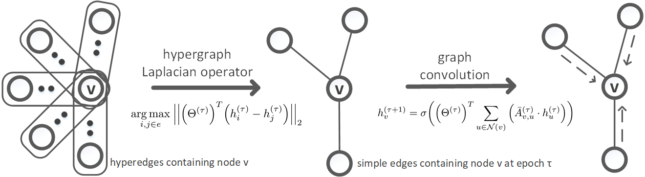
Figure 1: Graph convolution on a hypernode $v$ using HyperGCN.

4.1 Hypergraph Laplacian

As explained before, the key element for a GCN is the graph Laplacian of the given graph $\mathcal{G}$. Thus, in order to develop a GCN-based SSL method for hypergraphs, we first need to define a Laplacian for hypergraphs. One such way Chan et al. (2018) (see also Louis (2015)) is a non-linear function $\mathbb{L}:\mathbb{R}^{n}\rightarrow\mathbb{R}^{n}$ (the Laplacian matrix for graphs can be viewed as a linear function $L:\mathbb{R}^{n}\rightarrow\mathbb{R}^{n}$).

Definition 1 (Hypergraph Laplacian Chan et al. (2018); Louis (2015))

Given a real-valued signal $S\in\mathbb{R}^{n}$ defined on the hypernodes, $\mathbb{L}(S)$ is computed as follows.

1. For each hyperedge $e\in E$, let $(i_{e},j_{e})\coloneqq\text{argmax}_{i,j\in e}|S_{i}-S_{j}|$, breaking ties randomly.

2. A weighted graph $G_{S}$ on the vertex set $V$ is constructed by adding edges $\{\{i_{e},j_{e}\}:e\in E\}$ with weights $w(\{i_{e},j_{e}\})\coloneqq w(e)$ to $G_{S}$, where $w(e)$ is the weight of the hyperedge $e$. Next, to each vertex $v$, self-loops are added such that the degree of the vertex in $G_{S}$ is equal to $d_{v}$. Let $A_{S}$ denote the weighted adjacency matrix of the graph $G_{S}$.

3. The symmetrically normalised hypergraph Laplacian is ${\mathbb{L}}(S)\coloneqq(I-D^{-\frac{1}{2}}A_{S}D^{-\frac{1}{2}})S$

4.2 $1$-HyperGCN

By following the Laplacian construction steps outlined in Section 4.1, we end up with the simple graph $G_{S}$ with normalized adjacency matrix $\bar{A}_{S}$. We now perform GCN over this simple graph $G_{S}$. The graph convolution operation in Equation (1), when applied to a hypernode $v\in V$ in $G_{S}$, in the neural message-passing framework Gilmer et al. (2017) is $h_{v}^{(\tau+1)}=\sigma\bigg{(}(\Theta^{(\tau)})^{T}\sum_{u\in\mathcal{N}(v)}([\bar{A}^{(\tau)}_{S}]_{v,u}\cdot h^{(\tau)}_{u})\bigg{)}$. Here, $\tau$ is epoch number, $h^{(\tau+1)}_{v}$ is the new hidden layer representation of node $v$, $\sigma$ is a non-linear activation function, $\Theta$ is a matrix of learned weights, $\mathcal{N}(u)$ is the set of neighbours of $v$, $[\bar{A}^{(\tau)}_{S}]_{v,u}$ is the weight on the edge $\{v,u\}$ after normalisation, and $h^{(\tau)}_{u}$ is the previous hidden layer representation of the neighbour $u$. We note that along with the embeddings of the hypernodes, the adjacency matrix is also re-estimated in each epoch.

Figure 1 shows a hypernode $v$ with five hyperedges incident on it. We consider exactly one representative simple edge for each hyperedge $e\in E$ given by $(i_{e},j_{e})$ where $(i_{e},j_{e})=\operatorname*{arg\,max}_{i,j\in e}||(\Theta^{(\tau)})^{T}(h^{(\tau)}_{i}-h^{(\tau)}_{j})||_{2}$ for epoch $\tau$. Because of this consideration, the hypernode $v$ may not be a part of all representative simple edges (only three shown in figure). We then use traditional Graph Convolution Operation on $v$ considering only the simple edges incident on it. Note that we apply the operation on each hypernode $v\in V$ in each epoch $\tau$ of training until convergence.

Connection to total variation on hypergraphs: Our 1-HyperGCN model can be seen as performing implicit regularisation based on the total variation on hypergraphs Hein et al. (2013). In that prior work, explicit regularisation and only the hypergraph structure is used for hypernode classification in the SSL setting. HyperGCN, on the other hand, can use both the hypergraph structure and also exploit any available features on the hypernodes, e.g., text attributes for documents.

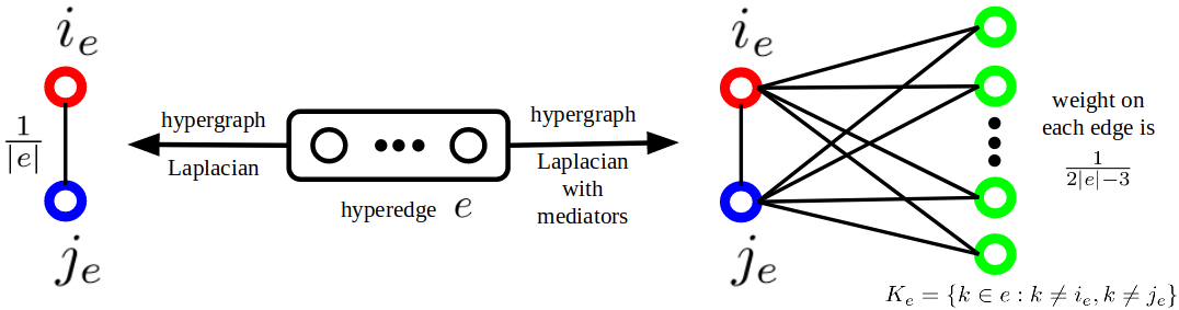
Figure 2: Hypergraph Laplacian Chan et al. (2018) vs. the generalised hypergraph Laplacian with mediators Chan and Liang (2018). Our approach requires at most a linear number of edges ($1$ and $2|e|-3$ respectively) while HGNN Feng et al. (2019) requires a quadratic number of edges for each hyperedge.

4.3 HyperGCN: Enhancing $1$-HyperGCN with mediators

One peculiar aspect of the hypergraph Laplacian discussed is that each hyperedge $e$ is represented by a single pairwise simple edge $\{i_{e},j_{e}\}$ (with this simple edge potentially changing from epoch to epoch). This hypergraph Laplacian ignores the hypernodes in $K_{e}:=\{k\in e:\ k\neq i_{e},k\neq j_{e}\}$ in the given epoch. Recently, it has been shown that a generalised hypergraph Laplacian in which the hypernodes in $K_{e}$ act as “mediators" Chan and Liang (2018) satisfies all the properties satisfied by the above Laplacian given by Chan et al. (2018). The two Laplacians are pictorially compared in Figure 2. Note that if the hyperedge is of size $2$, we connect $i_{e}$ and $j_{e}$ with an edge. We also run a GCN on the simple graph associated with the hypergraph Laplacian with mediators Chan and Liang (2018) (right in Figure 2). It has been suggested that the weights on the edges for each hyperedge in the hypergraph Laplacian (with mediators) sum to $1$ Chan and Liang (2018). We chose each weight to be $\frac{1}{2|e|-3}$ as there are $2|e|-3$ edges for a hyperedge $e$.

4.4 FastHyperGCN

We use just the initial features $X$ (without the weights) to construct the hypergraph Laplacian matrix (with mediators) and we call this method FastHyperGCN. Because the matrix is computed only once before training (and not in each epoch), the training time of FastHyperGCN is much less than that of other methods. We have provided the algorithms for the three methods in the supplementary.

5 Experiments for semi-supervised learning

We conducted experiments not only on real-world datasets but also on categorical data (results in supplementary) which are a standard practice in hypergraph-based learning Zhou et al. (2007); Hein et al. (2013); Zhang et al. (2017); Li and Milenkovic (2018b, a); Li et al. (2018a).

5.1 Baselines

We compared HyperGCN, $1$-HyperGCN and FastHyperGCN against the following baselines:

• Hypergraph neural networks (HGNN) Feng et al. (2019) uses the clique expansion Zhou et al. (2007); Agarwal et al. (2006) to approximate the hypergraph. Each hyperedge of size $s$ is approximated by an $s$-clique.

• Multi-layer perceptron (MLP) treats each instance (hypernode) as an independent and identically distributed (i.i.d) instance. In other words, $A=I$ in equation 1. We note that this baseline does not use the hypergraph structure to make predictions.

• Multi-layer perceptron + explicit hypergraph Laplacian regularisation (MLP + HLR): regularises the MLP by training it with the loss given by $\mathcal{L}=\mathcal{L}_{0}+\lambda\mathcal{L}_{reg}$ and uses the hypergraph Laplacian with mediators for explicit Laplacian regularisation $L_{reg}$. We used $10\%$ of the test set used for all the above models for this baseline to get an optimal $\lambda$.

• Confidence Interval-based method (CI) Zhang et al. (2017) uses a subgradient-based method Zhang et al. (2017). We note that this method has consistently been shown to be superior to the primal dual hybrid gradient (PDHG) of Hein et al. (2013) and also Zhou et al. (2007). Hence, we did not use these other previous methods as baselines, and directly compared HyperGCN against CI.

The task for each dataset is to predict the topic to which a document belongs (multi-class classification). Statistics are summarised in Table 3. For more details about datasets, please refer to the supplementary. We trained all methods for $200$ epochs and used the same hyperparameters of a prior work Kipf and Welling (2017). We report the mean test error and standard deviation over $100$ different train-test splits. We sampled sets of same sizes of labelled hypernodes from each class to have a balanced train split.

Table 3: Real-world hypergraph datasets used in our work. Distribution of hyperedge sizes is not symmetric either side of the mean and has a strong positive skewness.

	DBLP	Pubmed	Cora	Cora	Citeseer
	(co-authorship)	(co-citation)	(co-authorship)	(co-citation)	(co-citation)
# hypernodes, $|V|$	$43413$	$19717$	$2708$	$2708$	$3312$
# hyperedges, $|E|$	$22535$	$7963$	$1072$	$1579$	$1079$
avg.hyperedge size	$\mathbf{4.7\pm 6.1}$	$\mathbf{4.3\pm 5.7}$	$\mathbf{4.2\pm 4.1}$	$\mathbf{3.0\pm 1.1}$	$\mathbf{3.2\pm 2.0}$
# features, $d$	$1425$	$500$	$1433$	$1433$	$3703$
# classes, $q$	$6$	$3$	$7$	$7$	$6$
label rate, $|V_{L}|/|V|$	$0.040$	$0.008$	$0.052$	$0.052$	$0.042$

Table 4: Results of SSL experiments. We report mean test error $\pm$ standard deviation (lower is better) over $100$ train-test splits. Please refer to section 5 for details.

Data	Method	DBLP	Pubmed	Cora	Cora	Citeseer
		co-authorship	co-citation	co-authorship	co-citation	co-citation
$\mathbf{\mathcal{H}}$	CI	$54.81\pm 0.9$	$52.96\pm 0.8$	$55.45\pm 0.6$	$64.40\pm 0.8$	$70.37\pm 0.3$
$\mathbf{X}$	MLP	$37.77\pm 2.0$	$30.70\pm 1.6$	$41.25\pm 1.9$	$42.14\pm 1.8$	$41.12\pm 1.7$
$\mathbf{\mathcal{H},X}$	MLP + HLR	$30.42\pm 2.1$	$30.18\pm 1.5$	$34.87\pm 1.8$	$36.98\pm 1.8$	$37.75\pm 1.6$
$\mathbf{\mathcal{H},X}$	HGNN	$25.65\pm 2.1$	$29.41\pm 1.5$	$31.90\pm 1.9$	$\mathbf{32.41\pm 1.8}$	$\mathbf{37.40\pm 1.6}$
$\mathbf{\mathcal{H},X}$	1-HyperGCN	$33.87\pm 2.4$	$30.08\pm 1.5$	$36.22\pm 2.2$	$34.45\pm 2.1$	$38.87\pm 1.9$
$\mathbf{\mathcal{H},X}$	FastHyperGCN	$27.34\pm 2.1$	$29.48\pm 1.6$	$32.54\pm 1.8$	$\mathbf{32.43\pm 1.8}$	$\mathbf{37.42\pm 1.7}$
$\mathbf{\mathcal{H},X}$	HyperGCN	$\mathbf{24.09\pm 2.0}$	$\mathbf{25.56\pm 1.6}$	$\mathbf{30.08\pm 1.8}$	$\mathbf{32.37\pm 1.7}$	$\mathbf{37.35\pm 1.6}$

6 Analysis of results

The results on real-world datasets are shown in Table 4. We now attempt to explain them.

Proposition 1:

Given a hypergraph $\mathcal{H}=(V,E)$ with $E\subseteq 2^{V}-\cup_{v\in V}\{v\}$ and signals on the vertices $S:V\rightarrow{R}^{d}$, let, for each hyperedge $e\in E$, $(i_{e},j_{e}):=\operatorname*{arg\,max}_{i,j\in e}||S_{i}-S_{j}||_{2}$ and $K_{e}:=\{v\in e:v\neq i_{e},v\neq j_{e}\}$. Define

• $E_{c}:=\bigcup\limits_{e\in E}\Big{\{}\{u,v\}:u\in e,v\in e,u\neq v\Big{\}}$

• $w_{c}\Big{(}\{u,v\}\Big{)}:=\sum\limits_{e\in E}\mathbbm{1}_{\{u,v\}\in E_{c}}\cdot\mathbbm{1}_{u\in e}\cdot\mathbbm{1}_{v\in e}\Big{(}\frac{2}{|e|\cdot(|e|-1)}\Big{)},\quad$

• $E_{m}(S):=\bigcup\limits_{e\in E}\{i_{e},j_{e}\}\quad\bigcup\quad\bigcup\limits_{e\in E,|e|\geq 3}\Big{\{}\{u,v\}:u\in\{i_{e},j_{e}\},v\in K_{e}\big{\}}\Big{\}}$

• $w_{m}\Big{(}S,\{u,v\}\Big{)}:=\sum\limits_{e\in E}\mathbbm{1}_{\{u,v\}\in E_{m}(S)}\cdot\mathbbm{1}_{u\in e}\cdot\mathbbm{1}_{v\in e}\Big{(}\frac{1}{2|e|-3}\Big{)},\quad$

so that $G_{c}=(V,E_{c},w_{c})$ and $G_{m}(S)=(V,E_{m}(S),w_{m}(S))$ are the normalised clique exapnsion, i.e., graph of HGNN and mediator expansion, i.e., graph of HyperGCN/FastHyperGCN respectively. A sufficient condition for $G_{c}=G_{m}(S),\forall S$ is $\max\limits_{e\in E}|e|=3$.

Table 5: Results (lower is better) on sythetic data and a subset of DBLP showing that our methods are more effective for noisy hyperedges. $\eta$ is no. of hypernodes of one class divided by that of the other in noisy hyperedges. Best result is in bold and second best is underlined. Please see Section 6.

Method	$\eta=0.75$	$\eta=0.70$	$\eta=0.65$	$\eta=0.60$	$\eta=0.55$	$\eta=0.50$	sDBLP
HGNN	$\mathbf{15.92\pm 2.4}$	$\mathbf{24.89\pm 2.2}$	$\mathbf{31.32\pm 1.9}$	$39.13\pm 1.78$	$42.23\pm 1.9$	$44.25\pm 1.8$	$45.27\pm 2.4$
FastHyperGCN	$28.86\pm 2.6$	$31.56\pm 2.7$	$33.78\pm 2.1$	$\underline{33.89\pm 2.0}$	$\mathbf{34.56\pm 2.2}$	$\mathbf{35.65\pm 2.1}$	$\underline{41.79\pm 2.8}$
HyperGCN	$\underline{22.44\pm 2.0}$	$\underline{29.33\pm 2.2}$	$\underline{33.41\pm 1.9}$	$\mathbf{33.67\pm 1.9}$	$\underline{35.05\pm 2.0}$	$\underline{37.89\pm 1.9}$	$\mathbf{41.64\pm 2.6}$

Proof:

Observe that we consider hypergraphs in which the size of each hyperedge is at least $2$. It follows from definitions that $|E_{c}|=\sum_{e\in E}\ ^{|e|}C_{2}$ and $|E_{m}|=\sum_{e\in E}\Big{(}2|e|-3\Big{)}$. Clealy, a sufficient condition is when each hyperedge is approximated by the same subgraph in both the expansions. In other words the condition is $\frac{|e|\cdot(|e|-1)}{2}=2|e|-3$ for each $e\in E$. Solving the resulting quadratic eqution $x^{2}-5x+6=0$ gives us $(x-2)(x-3)=0$. Hence, $|e|=2$ or $|e|=3$ for each $e\in E$. $\square$

Comparable performance on Cora and Citeseer co-citation We note that HGNN is the most competitive baseline. Also $S=X$ for FastHyperGCN and $S=H\Theta$ for HyperGCN. The proposition states that the graphs of HGNN, FastHyperGCN, and HyperGCN are the same irrespective of the signal values whenever the maximum size of a hyperedge is $3$.

This explains why the three methods have comparable accuracies for Cora co-citaion and Citeseer co-citiation hypergraphs. The mean hyperedge sizes are close to $3$ (with comparitively lower deviations) as shown in Table 3. Hence the graphs of the three methods are more or less the same.

Superior performance on Pubmed, DBLP, and Cora co-authorship We see that HyperGCN performs statistically significantly (p-value of Welch t-test is less than 0.0001) compared to HGNN on the other three datasets. We believe this is due to large noisy hyperedges in real-world hypergraphs. An author can write papers from different topics in a co-authorship network or a paper typically cites papers of different topics in co-citation networks.

Average sizes in Table 3 show the presence of large hyperedges (note the large standard deviations). Clique expansion has edges on all pairs and hence potentially a larger number of hypernode pairs of different labels than the mediator graph of Figure 2, thus accumulating more noise.

Preference of HyperGCN and FastHyperGCN over HGNN To further illustrate superiority over HGNN on noisy hyperedges, we conducted experiments on synthetic hypergraphs each consisting of $1000$ hypernodes, randomly sampled $500$ hyperedges, and $2$ classes with $500$ hypernodes in each class. For each synthetic hypergraph, $100$ hyperedges (each of size $5$) were “pure", i.e., all hypernodes were from the same class while the other $400$ hyperedges (each of size $20$) contained hypernodes from both classes. The ratio, $\eta$, of hypernodes of one class to the other was varied from $0.75$ (less noisy) to $0.50$ (most noisy) in steps of $0.05$.

Table 5 shows the results on synthetic data. We initialise the hypernode features to random Gaussian of $256$ dimensions. We report mean error and deviation over $10$ different synthetically generated hypergraphs. As we can see in the table for hyperedges with $\eta=0.75,0.7$ (mostly pure), HGNN is the superior model. However, as $\eta$ (noise) increases our methods begin to outperform HGNN.

Subset of DBLP: We also trained all three models on a subset of DBLP (we call it sDBLP) by removing all hyperedges of size $2$ and $3$. The resulting hypergraph has around $8000$ hyperedges with an average size of $8.5\pm 8.8$. We report mean error over $10$ different train-test splits in Table 5.

Conclusion: From the above analysis, we conclude that our proposed methods (HyperGCN and FastHyperGCN) should be preferred to HGNN for hypergraphs with large noisy hyperedges. This is also the case on experiments in combinatorial optimisation (Table 6) which we discuss next.

7 HyperGCN for combinatorial optimisation

Inspired by the recent sucesses of deep graph models as learning-based approaches for NP-hard problems Li et al. (2018c); Prates et al. (2019); Lemos et al. (2019); Gong et al. (2019), we have used HyperGCN as a learning-based approach for the densest $k$-subhypergraph problem Chlamtác et al. (2018). NP-hard problems on hypergraphs have recently been highlighted as crucial for real-world network analysis Amburg et al. (2019); Nguyen et al. (2019). Our problem is, given a hypergraph $(V,E)$, to find a subset $W\subseteq V$ of $k$ hypernodes so as to maximise the number of hyperedges contained in $V$, i.e., we wish to maximise the density given by $|e\in E:e\subseteq W|$.

A greedy heuristic for the problem is to select the $k$ hypernodes of the maximum degree. We call this “MaxDegree". Another greedy heuristic is to iteratively remove all hyperedges from the current (residual) hypergraph consisting of a hypernode of the minimum degree. We repeat the procedure $n-k$ times and consider the density of the remaining $k$ hypernodes. We call this “RemoveMinDegree".

Table 6: Results on the densest $k$-subhypergraph problem. We report density (higher is better) of the set of vertices obtained by each of the proposed approaches for $k=\frac{3|V|}{4}$. See section 7 for details.

Dataset$\rightarrow$	Synthetic	DBLP	Pubmed	Cora	Cora	Citeseer
Approach$\downarrow$	test set	co-authorship	co-citation	co-authorship	co-citation	co-citation
MaxDegree	$174\pm 50$	$4840$	$1306$	$194$	$544$	$507$
RemoveMinDegree	$147\pm 48$	$\mathbf{7714}$	$\mathbf{7963}$	$450$	$1369$	$843$
MLP	$174\pm 56$	$5580$	$1206$	$238$	$550$	$534$
MLP + HLR	$231\pm 46$	$5821$	$3462$	$297$	$952$	$764$
HGNN	$337\pm 49$	$6274$	$7865$	$437$	$\mathbf{1408}$	$\mathbf{969}$
$1$-HyperGCN	$207\pm 52$	$5624$	$1761$	$251$	$563$	$509$
FastHyperGCN	$352\pm 45$	$7342$	$7893$	$452$	$\mathbf{1419}$	$\mathbf{969}$
HyperGCN	$\mathbf{359\pm 49}$	$\mathbf{7720}$	$\mathbf{7928}$	$\mathbf{504}$	$\mathbf{1431}$	$\mathbf{971}$
# hyperedges, $|E|$	$500$	$22535$	$7963$	$1072$	$1579$	$1079$

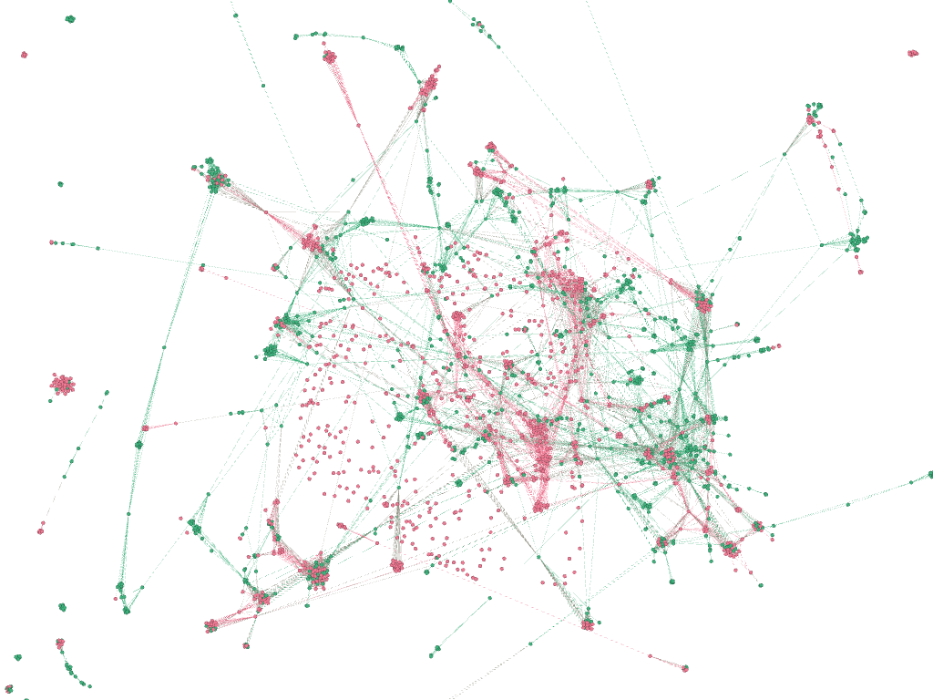
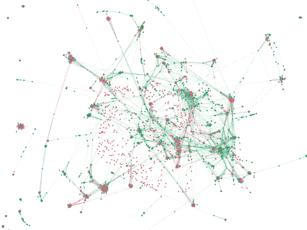
(a) RemoveMinDegree      (b) HyperGCN

Figure 3: Green / pink hypernodes denote those the algorithm labels as positive / negative respectively.

Experiments: Table 6 shows the results. We trained all the learning-based models with a synthetically generated dataset. More details on the approach and the synthetic data are in the supplementary. As seen in Table 6, our proposed HyperGCN outperforms all the other approaches except for the pubmed dataset which contains a small number of vertices with large degrees and a large number of vertices with small degrees. The RemoveMinDegree baseline is able to recover all the hyperedges here.

Qualitative analysis: Figure 3 shows the visualisations given by RemoveMinDegree and HyperGCN on the Cora co-authorship hypergraph. We used Gephi’s Force Atlas to space out the vertices. In general, a cluster of nearby vertices has multiple hyperedges connecting them. Clusters of only green vertices indicate the method has likely included all vertices within the hyperedges induced by the cluster. The figure of HyperGCN has more dense green clusters than that of RemoveMinDegree.

8 Comparison of training time

We compared the average training time of an epoch of FastHyperGCN and HGNN in Table 1. Both were run on a GeForce GTX 1080 Ti GPU machine. We observe that FastHyperGCN is faster than HGNN because it uses a linear number of edges for each hyperedge $e$ while HGNN uses quadratic. FastHyperGCN is also superior in terms of performance on hypergraphs with large noisy hyperedges.

9 Conclusion

We have proposed HyperGCN, a new method of training GCN on hypergraph using tools from spectral theory of hypergraphs. We have shown HyperGCN’s effectiveness in SSL and combinatorial optimisation. Approaches that assign importance to nodes Veličković et al. (2018); Monti et al. (2018); Vashishth et al. (2019b) have improved results on SSL. HyperGCN may be augmented with such approaches for even more improved performance. Supplementary: Hypergraph convolutional network

10 Algorithms of our proposed methods

The forward propagation of a $2$-layer graph convolutional network (GCN) Kipf and Welling (2017) is

$$Z=\text{softmax}\Bigg{(}\bar{A}\ \ \text{ReLU}\bigg{(}\bar{A}X\Theta^{(1)}\bigg{)}\Theta^{(2)}\Bigg{)}$$

$\text{ where }\ \ \bar{A}=\tilde{D}^{-\frac{1}{2}}\tilde{A}\tilde{D}^{-\frac{1}{2}},\quad\tilde{A}=A+I,\quad\text{and }\tilde{D}_{ii}=\sum_{j=1}^{N}\tilde{A}_{ij}$ and $D=\text{diag}(d_{1},\cdots,d_{N})$ is the diagonal degree matrix with elements $d_{i}=\sum_{j=1,j\neq i}^{N}A_{ji}$. We provide algorithms for our three proposed methods:

• HyperGCN - Algorithm 1

• FastHyperGCN - Algorithm 2

• 1-HyperGCN - Algorithm 3

Algorithm 1 Algorithm for HyperGCN

Input: An attributed hypergraph $\mathcal{H}=(V,E,X)$, with attributes $X$, a set of labelled vertices $\mathcal{V}_{L}$
      Output All hypernodes in $V-\mathcal{V}_{L}$ labelled

1:for each epoch $\tau$ of training do

2:     for layer $l=1,2$ of the network do

3:         set $A^{(l)}_{vv}=1$ For all hypernodes $v\in V$

4:         let $\Theta=\Theta^{\tau}$ be the parameters For the current epoch

5:         for $e\in E$ do

6:              $H\leftarrow$ hidden representation matrix of layer $l-1$

7:              $i_{e},j_{e}:=\text{argmax}_{i,j\in e}||H_{i}(\Theta^{(l)})-H_{j}(\Theta^{(l)})||_{2}$

8:              $A^{(l)}_{i_{e},j_{e}}=A^{(l)}_{j_{e},i_{e}}=\frac{1}{2|e|-3}$

9:              $K_{e}:=\{k\in e:\ k\neq i_{e},k\neq j_{e}\}$

10:              for $k\in K_{e}$ do

11:                  $A^{(l)}_{i_{e},k}=A^{(l)}_{k,i_{e}}=\frac{1}{2|e|-3}$

12:                  $A^{(l)}_{j_{e},k}=A^{(l)}_{k,j_{e}}=\frac{1}{2|e|-3}$

13:              end for

14:         end for

15:     end for

16:     $Z=\text{softmax}\Bigg{(}\bar{A}^{(2)}\ \ \text{ReLU}\bigg{(}\bar{A}^{(1)}X\Theta^{(1)}\bigg{)}\Theta^{(2)}\Bigg{)}$

17:     update parameters $\Theta^{\tau}$ to minimise cross entropy loss on the set of labelled hypernodes $\mathcal{V}_{L}$

18:end for

19:label the hypernodes in $V-\mathcal{V}_{L}$ using $Z$

Algorithm 2 Algorithm for FastHyperGCN

Input: An attributed hypergraph $\mathcal{H}=(V,E,X)$, with attributes $X$, a set of labelled vertices $\mathcal{V}_{L}$
      Output All hypernodes in $V-\mathcal{V}_{L}$ labelled

set $A_{vv}=1$ for all hypernodes $v\in V$

$i_{e},j_{e}:=\text{argmax}_{i,j\in e}||X_{i}-X_{j}||_{2}$

for $e\in E$ do

     $A_{i_{e},j_{e}}=A_{j_{e},i_{e}}=\frac{1}{2|e|-3}$

     $K_{e}:=\{k\in e:\ k\neq i_{e},k\neq j_{e}\}$

     for $k\in K_{e}$ do

         $A_{i_{e},k}=A_{k,i_{e}}=\frac{1}{2|e|-3}$

         $A_{j_{e},k}=A_{k,j_{e}}=\frac{1}{2|e|-3}$

     end for

end for

for each epoch $\tau$ of training do

     let $\Theta=\Theta^{\tau}$ be the parameters for the current epoch

     $Z=\text{softmax}\Bigg{(}\bar{A}\ \ \text{ReLU}\bigg{(}\bar{A}X\Theta^{(1)}\bigg{)}\Theta^{(2)}\Bigg{)}$

     update parameters $\Theta^{\tau}$ to minimise cross entropy loss on the set of labelled hypernodes $\mathcal{V}_{L}$

end for

label the hypernodes in $V-\mathcal{V}_{L}$ using $Z$

Algorithm 3 Algorithm for $1$-HyperGCN

Input: An attributed hypergraph $\mathcal{H}=(V,E,X)$, with attributes $X$, a set of labelled vertices $\mathcal{V}_{L}$
      Output All hypernodes in $V-\mathcal{V}_{L}$ labelled

for each epoch $\tau$ of training do

     for layer $l=1,2$ of the network do

         set $A^{(l)}_{vv}=1$ for all hypernodes $v\in V$

         let $\Theta=\Theta^{\tau}$ be the parameters for the current epoch

         for $e\in E$ do

              $H\leftarrow$ hidden representation matrix of layer $l-1$

              $i_{e},j_{e}:=\text{argmax}_{i,j\in e}||H_{i}(\Theta^{(l)})-H_{j}(\Theta^{(l)})||_{2}$

              $A^{(l)}_{i_{e},j_{e}}=A^{(l)}_{j_{e},i_{e}}=\frac{1}{|e|}$

         end for

     end for

     $Z=\text{softmax}\Bigg{(}\bar{A}^{(2)}\ \ \text{ReLU}\bigg{(}\bar{A}^{(1)}X\Theta^{(1)}\bigg{)}\Theta^{(2)}\Bigg{)}$

     update parameters $\Theta^{\tau}$ to minimise cross entropy loss on the set of labelled hypernodes $\mathcal{V}_{L}$

end for

label the hypernodes in $V-\mathcal{V}_{L}$ using $Z$

10.1 Time complexity

Given an attributed hypergraph $(V,E,X)$, let $d$ be the number of initial features, $h$ be the number of hidden units, and $l$ be the number of labels. Further, let $T$ be the total number of epochs of training. Define

$$N:=\sum_{e\in E}|e|,\quad\quad\quad N_{m}:=\sum_{e\in E}\Big{(}2|e|-3\Big{)},\quad\quad\quad N_{c}:=\sum_{e\in E}\ ^{|e|}C_{2}$$

• HyperGCN takes $O\bigg{(}T\Big{(}N+N_{m}h(d+c)\Big{)}\bigg{)}$ time

• 1-HyperGCN takes $O\bigg{(}TN\Big{(}1+h(d+c)\Big{)}\bigg{)}$ time

• FastHyperGCN takes $O\bigg{(}TN_{m}h\big{(}d+c\big{)}\bigg{)}$ time

• HGNN takes $O\bigg{(}TN_{c}h\big{(}d+c\big{)}\bigg{)}$ time

11 HyperGCN for combinatorial optimisation

Inspired by the recent sucesses of deep graph models as learning-based approaches for NP-hard problems Li et al. (2018c); Prates et al. (2019); Lemos et al. (2019); Gong et al. (2019), we have used HyperGCN as a learning-based approach for the densest $k$-subhypergraph problem Chlamtác et al. (2018), an NP-hard hypergraph problem. The problem is given a hypergraph $(V,E)$, find a subset $W\subseteq V$ of $k$ hypernodes so as to maximise the number of hyperedges contained in (induced by) $V$ i.e. we intend to maximise the density given by

$$|e\in E:e\subseteq W|$$

One natural greedy heuristic approach for the problem is to select the $k$ hypernodes of the maximum degree. We call this approach “MaxDegree". Another greedy heuristic approach is to iteratively remove all the hyperedges from the current (residual) hypergraph containing a hypernode of the minimum degree. We repeat the procedure $n-k$ times and consider the density of the remaining $k$ hypernodes. We call this approach “RemoveMinDegree".

11.1 Our approach

A natural approach to the problem is to train HyperGCN to perform the labelling. In other words, HyperGCN would take an input hypergraph $(V,E)$ as input and output a binary labelling of the hypernodes $v\in V$. A natural output representation is a probability map in $[0,1]^{|V|}$ that indicates how likely each hypernode is to belong to $W$.

Let $\mathcal{D}=\{(V_{i},E_{i}),l_{i}\}$ be a training set, where $(V_{i},E_{i})$ is an input hypergraph and $l_{i}\in\{0,1\}^{|V|\times 1}$ is one of the optimal solutions for the NP-hard hypergraph problem. The HyperGCN model learns its parameters $\Theta$ and is trained to predict $l_{i}$ given $(V_{i},E_{i})$. During training we minimise the binary cross-entropy loss $L$ for each training sample $\{(V_{i},E_{i}),l_{i}\}$ Additionally we generate $M$ different probability maps to minimise the hindsight loss i.e. $\sum_{i}\min_{m}L^{(m)}$ where $L^{(m)}$ is the cross-entropy loss corresponding to the $m$-th probability map. Generating multiple probability maps has the advantage of generating diverse solutions Li et al. (2018c).

11.2 Experiments: Training data

To generate a sample $\{(V,E),l\}$ in the training set $\mathcal{D}$, we fix a vertex set $W$ of $k$ vertices chosen uniformly randomly. We generate each hyperedge $e\in E$ such that $e\subseteq W$ with high probability $p$. Note that $e\subseteq V-W$ with probability $1-p$. We give the algorithm to generate a sample $\{(V,E),l\}$.

Algorithm 4 Algorithm for generating a training sample

Input: A hypergraph $(V,E)$ and a dense set of vertices $W$ $\mathcal{V}_{L}$
      Output A hypergraph $(V,E)$ and a dense set of vertices $W$

$|E|\leftarrow\frac{|V|}{2}$

$W\leftarrow$ subset of $V$ of size $k$ chosen uniformly randomly

for $i=1,2,\cdots,|E|$ do

     $|e|\sim\{2,3,\cdots 10\}$ chosen uniformly randomly

     sample $e$ from $W$ with probability $p$

     sample $e$ from $V-W$ with probability $1-p$

end for

11.3 Experiments: Results

We generated $5000$ training samples with the number of hypernodes $|V|$ uniformly randomly chosen from $\{1000,2000,\cdots,5000\}$. We fix $|E|=\frac{|V|}{2}$ as this is mostly the case for real-world hypergraphs. Further we chose $e\in E$ such that $|e|$ is uniformly randomly chosen from $\{2,\cdots,10\}$ as this is also mostly the case for real-world hypergraphs. We compared all our proposed approaches viz. $1$-HyperGCN, HyperGCN, and FastHyperGCN against the baselines MLP, MLP+HLR and the state-of-the art HGNN. We also compared against the greedy heuristics MaxDegree and RemoveMinDegree. We train all the deep models using the same hyperparameters of Li et al. (2018c) and report the results for $p=0.75$ and $k=\frac{3|V|}{4}$ in Table 7. We test all the models on a synthetically generated test set of hypergraphs with $1000$ vertices for each. We also test the models on the five real-world hypergraphs used for SSL experiments. As we can see in the table our proposed HyperGCN outperforms all the other approaches except for the pubmed dataset which contains a small number of vertices with large degrees and a large number of vertices with small degrees. The RemoveMinDegree baseline is able to recover all the hyperedges in the pubmed dataset. Moreover FastHyperGCN is competitive with HyperGCN as the number of hypergraphs in the training data is large.

11.4 Qualitative analysis

Figure 4 shows the visualisations given by RemoveMinDegree and HyperGCN on the Cora co-authorship hypergraph. We used Gephi’s Force Atlas to space out the vertices. In general, a cluster of nearby vertices has multiple hyperedges connecting them. Clusters of only green vertices indicate the method has likely included all vertices within the hyperedges induced by the cluster. The figure of HyperGCN has more dense green clusters than that of RemoveMinDegree. Figure 5 shows the results of HGNN vs. HyperGCN.

Table 7: Results on the densest $k$-subhypergraph problem. We report density (higher is better) of the set of vertices obtained by each of the proposed approaches for $k=\frac{3|V|}{4}$. See Section 11 for details.

Dataset$\rightarrow$	Synthetic	DBLP	Pubmed	Cora	Cora	Citeseer
Approach$\downarrow$	test set	co-authorship	co-citation	co-authorship	co-citation	co-citation
MaxDegree	$174\pm 50$	$4840$	$1306$	$194$	$544$	$507$
RemoveMinDegree	$147\pm 48$	$\mathbf{7714}$	$\mathbf{7963}$	$450$	$1369$	$843$
MLP	$174\pm 56$	$5580$	$1206$	$238$	$550$	$534$
MLP + HLR	$231\pm 46$	$5821$	$3462$	$297$	$952$	$764$
HGNN	$337\pm 49$	$6274$	$7865$	$437$	$\mathbf{1408}$	$\mathbf{969}$
$1$-HyperGCN	$207\pm 52$	$5624$	$1761$	$251$	$563$	$509$
FastHyperGCN	$352\pm 45$	$7342$	$7893$	$452$	$\mathbf{1419}$	$\mathbf{969}$
HyperGCN	$\mathbf{359\pm 49}$	$\mathbf{7720}$	$\mathbf{7928}$	$\mathbf{504}$	$\mathbf{1431}$	$\mathbf{971}$
# hyperedges, $|E|$	$500$	$22535$	$7963$	$1072$	$1579$	$1079$

(a) RemoveMinDegree      (b) HyperGCN

Figure 4: Green / pink hypernodes denote those the algorithm labels as positive / negative respectively.

(a) HGNN      (b) HyperGCN

Figure 5: Green / pink hypernodes denote those the algorithm labels as positive / negative respectively.

12 Sources of the real-world datasets

Co-authorship data: All documents co-authored by an author are in one hyperedge. We used the author datato get the co-authorship hypergraph for cora. We manually constructed the DBLP dataset from Arnetminer.

Co-citation data: All documents cited by a document are connected by a hyperedge. We used cora, citeseer, pubmed from for co-citation relationships. We removed hyperedges which had exactly one hypernode as our focus in this work is on hyperedges with two or more hypernodes. Each hypernode (document) is represented by bag-of-words features (feature matrix $X$).

12.1 Construction of the DBLP dataset

We downloaded the entire dblp data from https://aminer.org/lab-datasets/citation/DBLP-citation-Jan8.tar.bz. The steps for constructing the dblp dataset used in the paper are as follows:

• We defined a set of $6$ conference categories (classes for the SSL task) as “algorithms", “database", “programming", “datamining", “intelligence", and “vision"

• For a total of $4304$ venues in the entire dblp dataset we took papers from only a subset of venues from https://en.wikipedia.org/wiki/List_of_computer_science_conferences corresponding to the above $5$ conferences

• From the venues of the above $5$ conference categories, we got $22535$ authors publishing at least two documents for a total of $43413$

• We took the abstracts of all these $43413$ documents, constructed a dictionary of the most frequent words (words with frequency more than $100$) and this gave us a dictionary size of $1425$

13 Experiments on datasets with categorical attributes

Table 8: Summary of the three UCI datasets used in the experiments in Section 13

property/dataset	mushroom	covertype45	covertype67
number of hypernodes, $|V|$	$8124$	$12240$	$37877$
number of hyperedges, $|E|$	$112$	$104$	$125$
number of edges in clique expansion	$65,999,376$	$143,008,092$	$1,348,219,153$
number of classes, $q$	$2$	$2$	$2$

Figure 6: Test errors (lower is better) comparing HyperGCN_with_mediators with the non-neural baseline Zhang et al. (2017) on the UCI datasets. HyperGCN_with_mediators offers superior performance. Comparing against GCN on Clique Expansion is unfair. Please see below for details.

We closely followed the experimental setup of the baseline model Zhang et al. (2017). We experimented on three different datasets viz., mushroom, covertype45, and covertype67 from the UCI machine learning repository Dheeru and Karra Taniskidou (2017). Properties of the datasets are summarised in Table 8. The task for each of the three datasets is to predict one of two labels (binary classification) for each unlabelled instance (hypernode). The datasets contain instances with categorical attributes. To construct the hypergraph, we treat each attribute value as a hyperedge, i.e., all instances (hypernodes) with the same attribute value are contained in a hyperedge. Because of this particular definition of a hyperedge clique expansion is destined to produce an almost fully connected graph and hence GCN on clique expansion will be unfair to compare against. Having shown that HyperGCN is superior to $1$-HyperGCN in the relational experiments, we compare only the former and the non-neural baseline Zhang et al. (2017). We have calledHyperGCN as HyperGCN_with_mediators. We used the incidence matrix (that encodes the hypergraph structure) as the data matrix $X$. We trained HyperGCN_with_mediators for the full $200$ epochs and we used the same hyperparameters as in Kipf and Welling (2017).

As in Zhang et al. (2017), we performed $100$ trials for each $|V_{L}|$ and report the mean accuracy (averaged over the $100$ trials). The results are shown in Figure 6. We find that HyperGCN_with_mediators model generally does better than the baselines. We believe that this is because of the powerful feature extraction capability of HyperGCN_with_mediators.

13.1 GCN on clique expansion

We reiterate that clique expansion, i.e., HGNN Feng et al. (2019) for all the three datasets produce almost fuly connected graphs and hence clique expansion does not have any useful information. So, GCN on clique expansion is unfair to compare against (HGNN does not learn any useful weights for classification because of the fully connected nature of the graph).

13.2 Relevance of SSL

The main reason for performing these experiments, as pointed out in the publicly accessible NIPS reviews of the total variation on hypergraphs Hein et al. (2013), is to show that the proposed method (the primal-dual hybrid gradient method in their case and the HyperGCN_with_mediators method in our case) has improved results on SSL, even if SSL is not very relevant in the first place.

We do not claim that SSL with HyperGCN_with_mediators is the best way to go about handling these categorical data but we do claim that, given this built hypergraph albeit from non-relational data, it has superior results compared to the previous best non-neural hypergraph-based SSL method Zhang et al. (2017) in the literature and that is why we have followed their experimental setup.

14 Derivations

We show how the graph convolutional network (GCN) Kipf and Welling (2017) has its roots from the convolution theorem Mallat (1999).

Table 9: Results on Pubmed co-citation hypergraph. Mean test error $\pm$ standard deviation (lower is better) over $100$ trials for different values of $|V_{L}|$. We randomly sampled the same number of labelled hypernodes from each class and hence we chose each $|V_{L}|$ to be divisible by $q$ with $\frac{|V_{L}|}{|V|}$ $0.2$ to $1\%$.

Available data	Method	$\mathbf{39}$	$\mathbf{78}$	$\mathbf{120}$	$\mathbf{159}$	$\mathbf{198}$
		$\mathbf{0.2\%}$	$\mathbf{0.4\%}$	$\mathbf{0.6\%}$	$\mathbf{0.8\%}$	$\mathbf{1\%}$
$\mathbf{\mathcal{H}}$	CI	$62.61\pm 1.69$	$58.53\pm 1.25$	$55.71\pm 1.03$	$52.96\pm 0.79$	$50.21\pm 0.56$
$\mathbf{X}$	MLP	$43.85\pm 7.80$	$35.17\pm 4.92$	$32.04\pm 2.31$	$30.70\pm 1.61$	$28.87\pm 1.16$
$\mathbf{\mathcal{H},X}$	MLP + HLR	$42.31\pm 6.99$	$33.69\pm 4.49$	$31.79\pm 2.38$	$30.18\pm 1.54$	$28.09\pm 1.29$
$\mathbf{\mathcal{H},X}$	HGNN	$37.99\pm 6.45$	$33.01\pm 4.25$	$31.14\pm 2.23$	$29.41\pm 1.47$	$26.96\pm 1.35$
$\mathbf{\mathcal{H},X}$	1-HyperGCN	$43.62\pm 7.18$	$34.58\pm 4.24$	$31.88\pm 2.78$	$30.08\pm 1.53$	$28.90\pm 1.29$
$\mathbf{\mathcal{H},X}$	FastHyperGCN	$39.72\pm 6.45$	$32.67\pm 3.91$	$30.66\pm 2.45$	$29.48\pm 1.60$	$26.55\pm 1.31$
$\mathbf{\mathcal{H},X}$	HyperGCN	$\mathbf{33.33\pm 7.01}$	$\mathbf{31.71\pm 4.37}$	$\mathbf{28.84\pm 2.60}$	$\mathbf{25.56\pm 1.55}$	$\mathbf{23.97\pm 1.24}$

14.1 Graph signal processing

We now briefly review essential concepts of graph signal processing that are important in the construction of ChebNet and graph convolutional networks. We need convolutions on graphs defined in the spectral domain. Similar to regular $1$-D or $2$-D signals, real-valued graph signals can be efficiently analysed via harmonic analysis and processed in the spectral domain Shuman et al. (2013). To define spectral convolution, we note that the convolution theorem Mallat (1999) generalises from classical discrete signal processing to take into account arbitrary graphs Sandryhaila and Moura (2013).

Informally, the convolution theorem says the convolution of two signals in one domain (say time domain) equals point-wise multiplication of the signals in the other domain (frequency domain). More formally, given a graph signal, $S:\mathcal{V}\rightarrow\mathbb{R}$, $S\in\mathbb{R}^{N}$, and a filter signal, $F:\mathcal{V}\rightarrow\mathbb{R}$, $F\in\mathbb{R}^{N}$, both of which are defined in the vertex domain (time domain), the convolution of the two signals, $C=S\star F$, satisfies

$$\hat{C}=\hat{S}\odot\hat{F}$$ (3)

where $\hat{S}$, $\hat{F}$, $\hat{C}$ are the graph signals in the spectral domain (frequency domain) corresponding, respectively, to $S$, $F$ and $S\star F$.

An essential operator for computing graph signals in the spectral domain is the symmetrically normalised graph Laplacian operator of $\mathcal{G}$, defined as

$$L=I-D^{-\frac{1}{2}}AD^{-\frac{1}{2}}$$ (4)

where $D=\text{diag}(d_{1},\cdots,d_{N})$ is the diagonal degree matrix with elements $d_{i}=\sum_{j=1,j\neq i}^{N}A_{ji}$. As the above graph Laplacian operator, $L$, is a real symmetric and positive semidefinite matrix, it admits spectral eigen decomposition of the form $L=U\Lambda U^{T}$, where, $U=[u_{1},\cdots,u_{N}]$ forms an orthonormal basis of eigenvectors and $\Lambda=\text{diag}(\lambda_{1},\cdots,\lambda_{N})$ is the diagonal matrix of the corresponding eigenvalues with $0=\lambda_{1}\leq\cdots\leq\lambda_{N}\leq 2$.

The eigenvectors form a Fourier basis and the eigenvalues carry a notion of frequencies as in classical Fourier analysis. The graph Fourier transform of a graph signal $S=(S_{1},\cdots,S_{N})\in\mathbb{R}^{N}$, is thus defined as $\hat{S}=U^{T}S$ and the inverse graph Fourier transform turns out to be $S=U\hat{S}$ , which is the same as,

$$S_{i}=\sum_{j=1}^{N}\hat{S}(\lambda_{j})u_{j}(i)\quad\text{ for }\ i\in\mathcal{V}=\{1,\cdots,N\}$$ (5)

The convolution theorem generalised to graph signals  3 can thus be rewritten as $U^{T}C=\hat{S}\odot\hat{F}$. It follows that $C=U(\hat{S}\odot\hat{F})$, which is the same as

$$C_{i}=\sum_{j=1}^{N}\hat{S}(\lambda_{j})\hat{F}(\lambda_{j})u_{j}(i)\quad\text{ for }\ i\in\mathcal{V}=\{1,\cdots,N\}$$ (6)

Table 10: Results on DBLP co-authorship hypergraph. Mean test error $\pm$ standard deviation (lower is better) over $100$ trials for different values of $|V_{L}|$. We randomly sampled the same number of labelled hypernodes from each class and hence we chose each $|V_{L}|$ to be divisible by $q$ with $\frac{|V_{L}|}{|V|}$ $1$ to $5\%$.

Available data	Method	$\mathbf{438}$	$\mathbf{870}$	$\mathbf{1302}$	$\mathbf{1740}$	$\mathbf{2172}$
		$\mathbf{1\%}$	$\mathbf{2\%}$	$\mathbf{3\%}$	$\mathbf{4\%}$	$\mathbf{5\%}$
$\mathbf{\mathcal{H}}$	CI	$61.32\pm 1.58$	$59.39\pm 1.37$	$56.95\pm 1.12$	$54.81\pm 0.94$	$51.33\pm 0.66$
$\mathbf{X}$	MLP	$44.57\pm 7.19$	$42.23\pm 4.88$	$38.89\pm 3.62$	$37.77\pm 2.02$	$35.12\pm 1.57$
$\mathbf{\mathcal{H},X}$	MLP + HLR	$34.54\pm 7.49$	$33.50\pm 4.17$	$32.77\pm 3.16$	$30.42\pm 2.07$	$29.21\pm 1.94$
$\mathbf{\mathcal{H},X}$	HGNN	$30.62\pm 8.02$	$27.09\pm 4.48$	$26.18\pm 3.29$	$25.65\pm 2.08$	$\mathbf{24.02\pm 1.91}$
$\mathbf{\mathcal{H},X}$	1-HyperGCN	$40.17\pm 6.99$	$36.99\pm 4.78$	$34.44\pm 3.43$	$33.87\pm 2.39$	$32.11\pm 1.96$
$\mathbf{\mathcal{H},X}$	FastHyperGCN	$34.03\pm 7.59$	$29.93\pm 4.35$	$28.57\pm 3.13$	$27.34\pm 2.06$	$25.23\pm 1.84$
$\mathbf{\mathcal{H},X}$	HyperGCN	$\mathbf{28.51\pm 7.73}$	$\mathbf{25.45\pm 4.32}$	$\mathbf{24.69\pm 3.08}$	$\mathbf{24.09\pm 2.02}$	$\mathbf{23.96\pm 1.98}$

14.2 ChebNet convolution

We could use a non-parametric filter $\hat{F}(\lambda_{j})=\theta_{j}$  $\text{ for }\ j\in\{1,\cdots,N\}$ but there are two limitations: (i) they are not localised in space (ii) their learning complexity is $O(N)$. The two limitations above contrast with with traditional CNNs where the filters are localised in space and the learning complexity is independent of the input size. It is proposed by Defferrard et al. (2016) to use a polynomial filter to overcome the limitations. A polynomial filter is defined as:

$$\hat{F}(\lambda_{j})=\sum_{k=0}^{K}w_{k}\lambda_{j}^{k}\quad\text{ for }\ j\in\{1,\cdots,N\}$$ (7)

Using  7 in  6, we get $C_{i}=\sum_{j=1}^{N}\hat{S}(\lambda_{j})\bigg{(}\sum_{k=0}^{K}w_{k}\lambda_{j}^{k}\bigg{)}u_{j}(i)\quad\text{ for }\ i\in\mathcal{V}=\{1,\cdots,N\}$. From the definition of an eigenvalue, we have $Lu_{j}=\lambda_{j}u_{j}$ and hence $L^{k}u_{j}=\lambda_{j}^{k}u_{j}$ for a positive integer $k$ and $\text{ for }\ j\in\{1,\cdots,N\}$. Therefore,

$$\begin{split}C_{i}&=\sum_{j=1}^{N}\hat{S}(\lambda_{j})\bigg{(}\sum_{k=0}^{K}w_{k}L_{i}^{k}\bigg{)}u_{j}(i)\\ &=\bigg{(}\sum_{k=0}^{K}w_{k}L_{i}^{k}\bigg{)}\sum_{j=1}^{N}\hat{S}(\lambda_{j})u_{j}(i)\\ &=\bigg{(}\sum_{k=0}^{K}w_{k}L_{i}^{k}\bigg{)}S_{i}\end{split}$$ (8)

Hence,

$$\ \ C=\bigg{(}\sum_{k=0}^{K}w_{k}L^{k}\bigg{)}S$$ (9)

The graph convolution provided by Eq.  9 uses the monomial basis $1,x,\cdots,x^{K}$ to learn filter weights. Monomial bases are not optimal for training and not stable under perturbations because they do not form an orthogonal basis. It is proposed by Defferrard et al. (2016) to use the orthogonal Chebyshev polynomials Hammond et al. (2011) (and hence the name ChebNet) to recursively compute the powers of the graph Laplacian.

A Chebyshev polynomial $T_{k}(x)$ of order $k$ can be computed recursively by the stable recurrence relation $T_{k}(x)=2xT_{k-1}(x)-T_{k-2}(x)$ with $T_{0}=1$ and $T_{1}=x$. These polynomials form an orthogonal basis in $[-1,1]$. Note that the eigenvalues of the symmetrically normalised graph Laplacian  4 lie in the range $[0,2]$. Through appropriate scaling of eigenvalues from $[0,2]$ to $[-1,1]$ i.e. $\tilde{\lambda}_{j}=\frac{2\lambda_{j}}{\lambda_{N}}-1$ for $j=\{1,\cdots,N\}$, where $\lambda_{N}$ is the largest eigenvalue, the filter in  7 can be parametrised as the truncated expansion

$$\hat{F}(\lambda_{j})=\sum_{k=0}^{K}w_{k}T_{k}(\tilde{\lambda}_{j})\quad\text{ for }\ j\in\{1,\cdots,N\}$$ (10)

From Eq.  8, it follows that

$$C=\bigg{(}\sum_{k=0}^{K}w_{k}T_{k}(\tilde{L})\bigg{)}S\quad\text{where }\tilde{L}=\frac{2L}{\lambda_{N}}-I$$ (11)

Table 11: Results on Cora co-authorship hypergraph. Mean test error $\pm$ standard deviation (lower is better) over $100$ trials for different values of $|V_{L}|$. We randomly sampled the same number of labelled hypernodes from each class and hence we chose each $|V_{L}|$ to be divisible by $q$.

Available data	Method	$\mathbf{42}$	$\mathbf{98}$	$\mathbf{140}$	$\mathbf{203}$
$\mathbf{\mathcal{H}}$	CI	$67.72\pm 0.60$	$58.55\pm 0.53$	$55.45\pm 0.55$	$51.44\pm 0.32$
$\mathbf{X}$	MLP	$61.32\pm 4.86$	$47.69\pm 2.36$	$41.25\pm 1.85$	$37.76\pm 1.32$
$\mathbf{\mathcal{H},X}$	MLP + HLR	$54.31\pm 5.12$	$41.06\pm 2.53$	$34.87\pm 1.78$	$32.21\pm 1.43$
$\mathbf{\mathcal{H},X}$	HGNN	$45.23\pm 5.03$	$34.08\pm 2.40$	$31.90\pm 1.87$	$\mathbf{28.92\pm 1.49}$
$\mathbf{\mathcal{H},X}$	1-HyperGCN	$50.26\pm 4.78$	$39.01\pm 1.76$	$36.22\pm 2.21$	$32.78\pm 1.63$
$\mathbf{\mathcal{H},X}$	HyperGCN	$\mathbf{43.86\pm 4.78}$	$\mathbf{33.83\pm 1.81}$	$\mathbf{30.08\pm 1.80}$	$\mathbf{29.08\pm 1.44}$

14.3 Graph convolutional network (GCN): first-order approximation of ChebNet

The spectral convolution of  11 is $K$-localised since it is a $K^{th}$-order polynomial in the Laplacian i.e. it depends only on nodes that are at most $K$ hops away. Kipf and Welling (2017) simplify  11 to $K=1$ i.e. they use simple filters operating on $1$-hop neighbourhoods of the graph. More formally,

$$C=\bigg{(}w_{0}+w_{1}\tilde{L}\bigg{)}S$$ (12)

and also,

$$\hat{F}(\lambda_{j})=w_{0}+w_{1}\tilde{\lambda_{j}}\quad\text{ for }\ j\in\{1,\cdots,N\}$$ (13)

The main motivation here is that  12 is not limited to the explicit parameterisation given by the Chebyshev polynomials. Intuitively such a model cannot overfit on local neighbourhood structures for graphs with very wide node degree distributions, common in real-world graph datasets such as citation networks, social networks, and knowledge graphs.

In this formulation, Kipf and Welling (2017) further approximate $\lambda_{N}\approx 2$, as the neural network parameters can adapt to the change in scale during training. To address overfitting issues and to minimise the number of matrix multiplications, they set $w_{0}=-w_{1}=\theta$.  12 now reduces to

$$C=\theta(I-\tilde{L})S=\theta(2I-L)S=\theta(I+D^{-\frac{1}{2}}AD^{-\frac{1}{2}})S$$ (14)

The filter parameter $\theta$ is shared over the whole graph and successive application of a filter of this form $K$ times then effectively convolves the $K^{th}$-order neighbourhood of a node, where $K$ is the number of convolutional layers (depth) of the neural network model. We note that the eigenvalues of $L$ are in $[0,2]$ and hence the eigenvalues of $2I-L=I+D^{-\frac{1}{2}}AD^{-\frac{1}{2}}$ are also in the range $[0,2]$. Repeated application of this operator can therefore lead to numerical instabilities and exploding/vanishing gradients. To alleviate this problem, a renormalisation trick can be used Kipf and Welling (2017):

$$I+D^{-\frac{1}{2}}AD^{-\frac{1}{2}}\rightarrow\tilde{D}^{-\frac{1}{2}}\tilde{A}\tilde{D}^{-\frac{1}{2}}$$ (15)

$\text{with }\tilde{A}=A+I\quad\text{and }\tilde{D}_{ii}=\sum_{j=1}^{N}\tilde{A}_{ij}$. Generalising the above to $p$ signals contained in the matrix $X\in\mathbb{R}^{N\times p}$ (also called the data matrix), and $r$ filter maps contained in the matrix $\Theta\in\mathbb{R}^{p\times r}$, the output convolved signal matrix will be:

$$\bar{A}X\Theta\quad\text{ where }\bar{A}=\tilde{D}^{-\frac{1}{2}}\tilde{A}\tilde{D}^{-\frac{1}{2}}$$ (16)

Table 12: Results on Cora co-citation hypergraph. Mean test error $\pm$ standard deviation (lower is better) over $100$ trials for different values of $|V_{L}|$. We randomly sampled the same number of labelled hypernodes from each class and hence we chose each $|V_{L}|$ to be divisible by $q$.

Available data	Method	$\mathbf{42}$	$\mathbf{98}$	$\mathbf{140}$	$\mathbf{203}$
$\mathbf{\mathcal{H}}$	CI	$79.25\pm 1.34$	$70.89\pm 1.94$	$64.40\pm 0.81$	$62.22\pm 0.72$
$\mathbf{X}$	MLP	$63.31\pm 5.23$	$47.97\pm 3.15$	$42.14\pm 1.78$	$40.05\pm 1.58$
$\mathbf{\mathcal{H},X}$	MLP + HLR	$56.21\pm 5.65$	$43.32\pm 3.27$	$36.98\pm 1.83$	$33.88\pm 1.46$
$\mathbf{\mathcal{H},X}$	HGNN	$50.39\pm 5.42$	$\mathbf{35.62\pm 3.11}$	$\mathbf{32.41\pm 1.82}$	$\mathbf{29.78\pm 1.55}$
$\mathbf{\mathcal{H},X}$	1-HyperGCN	$50.39\pm 5.41$	$38.01\pm 3.12$	$34.45\pm 2.05$	$31.67\pm 1.57$
$\mathbf{\mathcal{H},X}$	HyperGCN	$\mathbf{47.00\pm 5.32}$	$\mathbf{35.76\pm 2.60}$	$\mathbf{32.37\pm 1.71}$	$\mathbf{29.98\pm 1.45}$

14.4 GCNs for graph-based semi-supervised node classification

The GCN is conditioned on both the adjacency matrix $A$ (underlying graph structure) and the data matrix $X$ (input features). This allows us to relax certain assumptions typically made in graph-based SSL, for example, the cluster assumption Chapelle et al. (2003) made by the explicit Laplacian-based regularisation methods. This setting is especially powerful in scenarios where the adjacency matrix contains information not present in the data (such as citation links between documents in a citation network or relations in a knowledge graph). The forward model for a simple two-layer GCN takes the following simple form:

$$Z=f_{GCN}(X,A)=\text{softmax}\Bigg{(}\bar{A}\ \ \text{ReLU}\bigg{(}\bar{A}X\Theta^{(0)}\bigg{)}\Theta^{(1)}\Bigg{)}$$ (17)

where $\Theta^{(0)}\in\mathbb{R}^{p\times h}$ is an input-to-hidden weight matrix for a hidden layer with $h$ hidden units and $\Theta^{(1)}\in\mathbb{R}^{h\times r}$ is a hidden-to-output weight matrix. The softmax activation function defined as $\text{softmax}(x_{i})=\frac{\text{exp}(x_{i})}{\sum_{i}\text{exp}(x_{i})}$ is applied row-wise.

Training

For semi-supervised multi-class classification with $q$ classes, we then evaluate the cross-entropy error over all the set of labelled examples, $\mathcal{V}_{L}$:

$$\mathcal{L}=-\sum_{i\in\mathcal{V}_{L}}\sum_{j=1}^{q}Y_{ij}\ln Z_{ij}$$ (18)

The weights of the graph convolutional network, viz. $\Theta^{(0)}$ and $\Theta^{(1)}$, are trained using gradient descent. Using efficient sparse-dense matrix multiplications for computing, the computational complexity of evaluating Eq.  17 is $O(|\mathcal{E}|phr)$ which is linear in the number of graph edges.

14.5 GCN as a special form of Laplacian smoothing

GCNs can be interpreted as a special form of symmetric Laplacian smoothing Li et al. (2018b). The Laplacian smoothing Taubin (1995) on each of the $p$ input channels in the input feature matrix $X\in\mathbb{R}^{N\times p}$ is defined as:

$$\chi_{i}=(1-\gamma)x_{i}+\gamma\sum_{j}\frac{\tilde{A}_{ij}}{d_{i}}x_{j}\quad i=1,\cdots,N$$ (19)

here $\tilde{A}=A+I$ and $d_{i}$ is the degree of node $i$. Equivalently the Laplacian smoothing can be written as $\chi=X-\gamma\tilde{D}^{-1}\tilde{L}X=(I-\gamma\tilde{D}^{-1}\tilde{L})X$ where $\tilde{L}=\tilde{D}-\tilde{A}$. Here $0\leq\gamma\leq 1$ is a parameter which controls the weighting between the feature of the current vertex and those of its neighbours. If we let $\gamma=1$, and replace the normalised Laplacian $\tilde{D}^{-1}\tilde{L}$ by the symmetrically normalised Laplacian $\tilde{D}^{-\frac{1}{2}}\tilde{L}\tilde{D}^{-\frac{1}{2}}$, then $\chi=(I-\tilde{D}^{-\frac{1}{2}}\tilde{L}\tilde{D}^{-\frac{1}{2}})X=\bar{A}X$, the same as in the expression  16.

Hence the graph convolution in the GCN is a special form of (symmetric) Laplacian smoothing. The Laplacian smoothing of Eq.  19 computes the new features of a node as the weighted average of itself and its neighbours. Since nodes in the same cluster tend to be densely connected, the smoothing makes their features similar, which makes the subsequent classification task much easier. Repeated application of Laplacian smoothing many times over leads to over-smoothing - the node features within each connected component of the graph will converge to the same values Li et al. (2018b).

15 Hyperparameters and more experiments on SSL

Please see tables 9, 10, 11, 12, and 13 for the results on all the real-world hypergraph datasets.

Following a prior work Kipf and Welling (2017), we used the following hyperparameters for all the models:

• hidden layer size: $32$

• dropout rate: $0.5$

• learning rate: $0.01$

• weight decay: $0.0005$

• number of training epochs: $200$

• $\lambda$ for explicit Laplacian regularisation: $0.001$

Table 13: Results on Citeseer co-citation hypergraph. Mean test error $\pm$ standard deviation (lower is better) over $100$ trials for different values of $|V_{L}|$. We randomly sampled the same number of labelled hypernodes from each class and hence we chose each $|V_{L}|$ to be divisible by $q$.

Available data	Method	$\mathbf{42}$	$\mathbf{102}$	$\mathbf{138}$	$\mathbf{198}$
$\mathbf{\mathcal{H}}$	CI	$74.68\pm 1.02$	$71.90\pm 0.82$	$70.37\pm 0.29$	$68.84\pm 0.24$
$\mathbf{X}$	MLP	$57.14\pm 4.87$	$45.80\pm 2.43$	$41.12\pm 1.65$	$39.09\pm 1.32$
$\mathbf{\mathcal{H},X}$	MLP + HLR	$53.21\pm 4.65$	$43.21\pm 2.35$	$37.75\pm 1.59$	$36.01\pm 1.29$
$\mathbf{\mathcal{H},X}$	HGNN	$\mathbf{50.75\pm 4.73}$	$\mathbf{39.67\pm 2.21}$	$\mathbf{37.40\pm 1.61}$	$\mathbf{35.20\pm 1.35}$
$\mathbf{\mathcal{H},X}$	1-HyperGCN	$52.48\pm 5.43$	$41.26\pm 2.54$	$38.87\pm 1.93$	$36.46\pm 1.46$
$\mathbf{\mathcal{H},X}$	HyperGCN	$\mathbf{50.39\pm 5.13}$	$\mathbf{39.68\pm 2.27}$	$\mathbf{37.35\pm 1.62}$	$\mathbf{35.40\pm 1.22}$

References

- Agarwal et al. (2006) Sameer Agarwal, Kristin Branson, and Serge Belongie. Higher order learning with graphs. In International Conference on Machine Learning (ICML), pages 17–24, 2006.
- Amburg et al. (2019) Ilya Amburg, Jon Kleinberg, and Austin R. Benson. Planted hitting set recovery in hypergraphs. CoRR, arXiv:1905.05839, 2019.
- Atwood and Towsley (2016) James Atwood and Don Towsley. Diffusion-convolutional neural networks. In Neural Information Processing Systems (NIPS), pages 1993–2001. Curran Associates, Inc., 2016.
- Battaglia et al. (2018) Peter W. Battaglia, Jessica Hamrick, Victor Bapst, Alvaro Sanchez-Gonzalez, Vinícius Flores Zambaldi, Mateusz Malinowski, Andrea Tacchetti, David Raposo, Adam Santoro, Ryan Faulkner, Çaglar Gülçehre, Francis Song, Andrew Ballard, Justin Gilmer, George Dahl, Ashish Vaswani, Kelsey Allen, Charles Nash, Victoria Langston, Chris Dyer, Nicolas Heess, Daan Wierstra, Pushmeet Kohli, Matthew Botvinick, Oriol Vinyals, Yujia Li, and Razvan Pascanu. Relational inductive biases, deep learning, and graph networks. arXiv:1806.01261, 2018.
- Bronstein et al. (2017) Michael Bronstein, Joan Bruna, Yann LeCun, Arthur Szlam, and Pierre Vandergheynst. Geometric deep learning: Beyond euclidean data. IEEE Signal Process., 34:18–42, 2017.
- Bulò and Pelillo (2009) Samuel R. Bulò and Marcello Pelillo. A game-theoretic approach to hypergraph clustering. In Advances in Neural Information Processing Systems (NIPS) 22, pages 1571–1579. Curran Associates, Inc., 2009.
- Chan and Liang (2018) T.-H. Hubert Chan and Zhibin Liang. Generalizing the hypergraph laplacian via a diffusion process with mediators. In Computing and Combinatorics - 24th International Conference, (COCOON), pages 441–453, 2018.
- Chan et al. (2018) T.-H. Hubert Chan, Anand Louis, Zhihao Gavin Tang, and Chenzi Zhang. Spectral properties of hypergraph laplacian and approximation algorithms. J. ACM, 65(3):15:1–15:48, 2018.
- Chapelle et al. (2003) Olivier Chapelle, Jason Weston, and Bernhard Schölkopf. Cluster kernels for semi-supervised learning. In Neural Information Processing Systems (NIPS), pages 601–608. MIT, 2003.
- Chapelle et al. (2010) Olivier Chapelle, Bernhard Scholkopf, and Alexander Zien. Semi-Supervised Learning. The MIT Press, 2010.
- Chen et al. (2019) Zhao-Min Chen, Xiu-Shen Wei, Peng Wang, and Yanwen Guo. Multi-label image recognition with graph convolutional networks. In The IEEE Conference on Computer Vision and Pattern Recognition (CVPR), 2019.
- Chien et al. (2019) I (Eli) Chien, Huozhi Zhou, and Pan Li. : Active learning over hypergraphs with pointwise and pairwise queries. In International Conference on Artificial Intelligence and Statistics (AISTATS), pages 2466–2475, 2019.
- Chlamtác et al. (2018) Eden Chlamtác, Michael Dinitz, Christian Konrad, Guy Kortsarz, and George Rabanca. The densest k-subhypergraph problem. SIAM J. Discrete Math., pages 1458–1477, 2018.
- Defferrard et al. (2016) Michaël Defferrard, Xavier Bresson, and Pierre Vandergheynst. Convolutional neural networks on graphs with fast localized spectral filtering. In Advances in Neural Information Processing Systems (NIPS), pages 3844–3852. Curran Associates, Inc., 2016.
- Dheeru and Karra Taniskidou (2017) Dua Dheeru and Efi Karra Taniskidou. UCI machine learning repository, 2017. URL http://archive.ics.uci.edu/ml.
- Feng et al. (2018) Fuli Feng, Xiangnan He, Yiqun Liu, Liqiang Nie, and Tat-Seng Chua. Learning on partial-order hypergraphs. In Proceedings of the 2018 World Wide Web Conference (WWW), pages 1523–1532, 2018.
- Feng et al. (2019) Yifan Feng, Haoxuan You, Zizhao Zhang, Rongrong Ji, and Yue Gao. Hypergraph neural networks. In Proceedings of the Thirty-Third Conference on Association for the Advancement of Artificial Intelligence (AAAI), 2019.
- Gilmer et al. (2017) Justin Gilmer, Samuel S. Schoenholz, Patrick F. Riley, Oriol Vinyals, and George E. Dahl. Neural message passing for quantum chemistry. In Proceedings of the 34th International Conference on Machine Learning (ICML), pages 1263–1272, 2017.
- Gong et al. (2019) Yu Gong, Yu Zhu, Lu Duan, Qingwen Liu, Ziyu Guan, Fei Sun, Wenwu Ou, and Kenny Q. Zhu. Exact-k recommendation via maximal clique optimization. In Proceedings of the 25th ACM SIGKDD International Conference on Knowledge Discovery & Data Mining (KDD), 2019.
- Hamilton et al. (2017) William L. Hamilton, Rex Ying, and Jure Leskovec. Representation learning on graphs: Methods and applications. IEEE Data Eng. Bull., 40(3):52–74, 2017.
- Hammond et al. (2011) David K. Hammond, Pierre Vandergheynst, and Rémi Gribonval. Wavelets on graphs via spectral graph theory. Applied and Computational Harmonic Analysis, 2011.
- Hein et al. (2013) Matthias Hein, Simon Setzer, Leonardo Jost, and Syama Sundar Rangapuram. The total variation on hypergraphs - learning on hypergraphs revisited. In Advances in Neural Information Processing Systems (NIPS) 26, pages 2427–2435. Curran Associates, Inc., 2013.
- Kipf and Welling (2017) Thomas N Kipf and Max Welling. Semi-supervised classification with graph convolutional networks. In International Conference on Learning Representations (ICLR), 2017.
- Kolda and Bader (2009) Tamara G. Kolda and Brett W. Bader. Tensor decompositions and applications. SIAM Rev., 51(3):455–500, 2009.
- Lemos et al. (2019) Henrique Lemos, Marcelo Prates, Pedro Avelar, and Luis Lamb. Graph colouring meets deep learning: Effective graph neural network models for combinatorial problems. In Proceedings of the 28th International Joint Conference on Artificial Intelligence, (IJCAI), 2019.
- Li and Milenkovic (2018a) Pan Li and Olgica Milenkovic. Revisiting decomposable submodular function minimization with incidence relations. In Advances in Neural Information Processing Systems (NeurIPS) 31, pages 2237–2247. Curran Associates, Inc., 2018a.
- Li and Milenkovic (2018b) Pan Li and Olgica Milenkovic. Submodular hypergraphs: p-laplacians, Cheeger inequalities and spectral clustering. In Proceedings of the 35th International Conference on Machine Learning (ICML), pages 3014–3023, 2018b.
- Li et al. (2018a) Pan Li, Niao He, and Olgica Milenkovic. Quadratic decomposable submodular function minimization. In Advances in Neural Information Processing Systems (NeurIPS) 31, pages 1054–1064. Curran Associates, Inc., 2018a.
- Li et al. (2018b) Qimai Li, Zhichao Han, and Xiao-Ming Wu. Deeper insights into graph convolutional networks for semi-supervised learning. In Proceedings of the Thirty-Second Conference on Association for the Advancement of Artificial Intelligence (AAAI), pages 3538–3545, 2018b.
- Li et al. (2018c) Zhuwen Li, Qifeng Chen, and Vladlen Koltun. Combinatorial optimization with graph convolutional networks and guided tree search. In Advances in Neural Information Processing Systems (NIPS) 31, pages 537–546. Curran Associates, Inc., 2018c.
- Louis (2015) Anand Louis. Hypergraph markov operators, eigenvalues and approximation algorithms. In Proceedings of the Forty-Seventh Annual ACM on Symposium on Theory of Computing, (STOC), pages 713–722, 2015.
- Mallat (1999) Stphane Mallat. A Wavelet Tour of Signal Processing. Academic Press, 1999.
- Marcheggiani and Titov (2017) Diego Marcheggiani and Ivan Titov. Encoding sentences with graph convolutional networks for semantic role labeling. In Proceedings of the 2017 Conference on Empirical Methods in Natural Language Processing (EMNLP), pages 1506–1515, 2017.
- Monti et al. (2018) Federico Monti, Oleksandr Shchur, Aleksandar Bojchevski, Or Litany, Stephan Günnemann, and Michael Bronstein. Dual-primal graph convolutional networks. abs/1806.00770, 2018.
- Nguyen et al. (2019) Hung Nguyen, Phuc Thai, My Thai, Tam Vu, and Thang Dinh. Approximate k-cover in hypergraphs: Efficient algorithms, and applications. CoRR, arXiv:1901.07928, 2019.
- Norcliffe-Brown et al. (2018) Will Norcliffe-Brown, Efstathios Vafeias, and Sarah Parisot. Learning conditioned graph structures for interpretable visual question answering. In Advances in Neural Information Processing Systems (NeurIPS) 31, pages 8344–8353. Curran Associates, Inc., 2018.
- Prates et al. (2019) Marcelo O. R. Prates, Pedro H. C. Avelar, Henrique Lemos, Luis Lamb, and Moshe Vardi. Learning to solve np-complete problems - a graph neural network for the decision tsp. In Proceedings of the Thirty-Third Conference on Association for the Advancement of Artificial Intelligence (AAAI), 2019.
- Sandryhaila and Moura (2013) Aliaksei Sandryhaila and José M. F. Moura. Discrete signal processing on graphs. IEEE Trans. Signal Processing, 2013.
- Satchidanand et al. (2015) Sai Nageswar Satchidanand, Harini Ananthapadmanaban, and Balaraman Ravindran. Extended discriminative random walk: A hypergraph approach to multi-view multi-relational transductive learning. In Proceedings of the Twenty-Fourth International Joint Conference on Artificial Intelligence, (IJCAI), pages 3791–3797, 2015.
- Shashua et al. (2006) Amnon Shashua, Ron Zass, and Tamir Hazan. Multi-way clustering using super-symmetric non-negative tensor factorization. In Proceedings of the 9th European Conference on Computer Vision (ECCV), pages 595–608, 2006.
- Shuman et al. (2013) David I. Shuman, Sunil K. Narang, Pascal Frossard, Antonio Ortega, and Pierre Vandergheynst. The emerging field of signal processing on graphs: Extending high-dimensional data analysis to networks and other irregular domains. IEEE Signal Process. Mag., 30(3), 2013.
- Subramanya and Talukdar (2014) Amarnag Subramanya and Partha Pratim Talukdar. Graph-Based Semi-Supervised Learning. Morgan & Claypool Publishers, 2014.
- Sun et al. (2018) Lichao Sun, Ji Wang, Philip S. Yu, and Bo Li. Adversarial attack and defense on graph data: A survey. CoRR, arXiv:1812.10528, 2018.
- Taubin (1995) Gabriel Taubin. A signal processing approach to fair surface design. In Proceedings of the 22Nd Annual Conference on Computer Graphics and Interactive Techniques, 1995.
- Vashishth et al. (2019a) Shikhar Vashishth, Manik Bhandari, Prateek Yadav, Piyush Rai, Chiranjib Bhattacharyya, and Partha Talukdar. Incorporating syntactic and semantic information in word embeddings using graph convolutional networks. In Proceedings of the 57th Annual Meeting of the Association for Computational Linguistics (ACL), 2019a.
- Vashishth et al. (2019b) Shikhar Vashishth, Prateek Yadav, Manik Bhandari, and Partha Talukdar. Confidence-based graph convolutional networks for semi-supervised learning. In International Conference on Artificial Intelligence and Statistics (AISTATS), 2019b.
- Veličković et al. (2018) Petar Veličković, Guillem Cucurull, Arantxa Casanova, Adriana Romero, Pietro Liò, and Yoshua Bengio. Graph attention networks. In International Conference on Learning Representations (ICLR), 2018.
- Wang et al. (2018) Xiaolong Wang, Yufei Ye, and Abhinav Gupta. Zero-shot recognition via semantic embeddings and knowledge graphs. In The IEEE Conference on Computer Vision and Pattern Recognition (CVPR), pages 6857–6866, 2018.
- Weston et al. (2008) Jason Weston, Frédéric Ratle, and Ronan Collobert. Deep learning via semi-supervised embedding. In Proceedings of the 25th International Conference on Machine Learning (ICML), pages 1168–1175, 2008.
- Wu et al. (2019) Zonghan Wu, Shirui Pan, Fengwen Chen, Guodong Long, Chengqi Zhang, and Philip S. Yu. A comprehensive survey on graph neural networks. CoRR, arXiv:1901.00596, 2019.
- Yao et al. (2019) Liang Yao, Chengsheng Mao, and Yuan Luo. Graph convolutional networks for text classification. In Proceedings of the Thirty-Third Conference on Association for the Advancement of Artificial Intelligence (AAAI), 2019.
- Zhang et al. (2017) Chenzi Zhang, Shuguang Hu, Zhihao Gavin Tang, and T-H. Hubert Chan. Re-revisiting learning on hypergraphs: Confidence interval and subgradient method. In Proceedings of 34th International Conference on Machine Learning (ICML), pages 4026–4034, 2017.
- Zhang et al. (2018) Ziwei Zhang, Peng Cui, and Wenwu Zhu. Deep learning on graphs: A survey. CoRR, arXiv:1812.04202, 2018.
- Zhou et al. (2003) Dengyong Zhou, Olivier Bousquet, Thomas Navin Lal, Jason Weston, and Bernhard Schölkopf. Learning with local and global consistency. In NIPS, 2003.
- Zhou et al. (2007) Denny Zhou, Jiayuan Huang, and Bernhard Schölkopf. Learning with hypergraphs: Clustering, classification, and embedding. In Advances in Neural Information Processing Systems (NIPS) 19, pages 1601–1608. MIT Press, 2007.
- Zhu et al. (2003) Xiaojin Zhu, Zoubin Ghahramani, and John Lafferty. Semi-supervised learning using gaussian fields and harmonic functions. In ICML, 2003.
- Zhu et al. (2009) Xiaojin Zhu, Andrew B. Goldberg, Ronald Brachman, and Thomas Dietterich. Introduction to Semi-Supervised Learning. Morgan and Claypool Publishers, 2009.