The dynamics of twisted disc formed after the tidal disruption of a star by a rotating black hole

Abstract

We consider misaligned accretion discs formed after tidal disruption events occurring when a star encounters a supermassive rotating black hole. We use the linear theory of warped accretion discs to find the disc shape when the stream produced by the disrupted star provides a source of mass and angular momentum that is misaligned with the black hole. The evolution of the surface density and aspect ratio is found from a one dimensional vertically averaged model.

We extend previous work which assumed a quasi-stationary disc to allow unrestricted dynamical propagation of disc tilt and twist through time dependent backgrounds. We consider a smaller value of the viscosity parameter, $\alpha=0.01,$ finding the dynamics varies significantly.

At early times the disc inclination is found to be nearly uniform at small radii where the aspect ratio is large. However, since torques arise from the Lense-Thirring effect and the stream there is non uniform precession. We propose a simple model for this requiring only the background surface density and aspect ratio.

At these times the $\alpha\sim 0.01$ disc exhibits a new feature. An inclined hot inner region joins an outer low inclination cool region via a thin transition front propagating outwards with a speed exceeding that of bending waves in the cool region. These waves accumulate where the propagation speeds match producing an inclination spike separating inner and outer discs. At late times a sequence of quasi-stationary configurations approximates disc shapes at small radii. We discuss observational implications of our results.

1 Introduction

The tidal disruption of stars by supermassive black holes (tidal disruption events, TDEs) is expected to result in accretion of stellar gas onto them and, accordingly, in an increase in their activity as suggested by Hills (1975). Over the last two decades or so TDEs have been proposed to explain non-stationary radiation flares observed in several dozen of galactic centres in different wavebands (from radio to X-rays), typically lasting for several years, (see e.g. Komossa, 2015)

1.1 Background

Recent understanding of a single TDE is based on the following simple picture proposed in Lacy et al. (1982) and Rees (1988). It is assumed that all stars with periastron distances, $R_{p}$, smaller that so-called tidal disruption radius, $R_{T}$, are disrupted by the tidal field the of black hole. Physically $R_{T}$ is defined by the condition that within a uniform density sphere of radius, $R_{T},$ and mass, $M,$ equal to that of the black hole, the density is the same as the mean density of the unperturbed star. It is given by equation (1) below. When the star is located at $R_{T},$ tidal forces and self-gravitational forces are expected to balance on rhe stellar surface with tidal forces being larger when the star is at smaller radii. Accordingly a star moving on a nearly parabolic orbit with $R_{p}<R_{T}$ is expected to become gravitationally unbound near periastron, (see e.g. Carter & Luminet, 1983, 1985; Khokhlov et al., 1993b; Ivanov & Novikov, 2001; Ivanov et al., 2003; Lodato et al., 2009; Guillochon & Ramirez-Ruiz, 2013, 2015) for different numerical models of this process.

Since the stellar centre of mass has zero binding energy on a parabolic orbit, stellar material that becomes closer to the black hole at periastron has positive binding energy and will accordingly be gravitationally bound to it. On the other hane, material which is further from the black hole at periastron will not be bound to it and thus expelled from the black hole. Accordingly, approximately one half of the stellar material will begin to move around the black hole on highly elliptical orbits with periods determined by the distribution of its mass with binding energy, which is often assumed to be uniform, (e.g Rees, 1988). Since different stellar fluid elements return to periastron at different times, there will be a stream of gas coming to periastron with associated mass flux, $\dot{M}_{S}$ equal to ${(m/3P_{min})}({t/P_{min}})^{-5/3}$, where $m$ is mass of the star and $P_{min}$ is the minimal return time to periastron for a gas element, which is nearest to the black hole at the time of periastron passage, which is given by equation (2) below.

Since the gas stream tends to intersect itself near $R_{p}$, on account of differential Einstein precession, gas circularises there and eventually forms an accretion disc or torus. Recent numerical simulations suggest that it takes a time $1-10P_{min}$ for an accretion disc structure to be formed near $R_{P}$, (see e.g. Hayasaki et al., 2013; Bonnerot et al., 2016). Initially such a disc, being in an advective state, accretes at a superEddington rate. But, after some time (typically, order of a year) has passed, it evolves into a ’standard’ optically thick, geometrically thin, radiative accretion disc, (see e.g. Shen & Matzner, 2014) and references therein. Such a disc differs, however, from the standard stationary accretion disc described in Shakura & Sunyaev (1973) by having a free outer boundary, its non-stationary nature and mass and energy input being provided by the stream.

An important aspect of the problem arises when the black hole rotates. Apart from modification of the disc spectrum, issues related to possible jet formation through the Blandford $\&$Znajek process and modification of the process of tidal disruption itself (e.g. Ivanov & Chernyakova, 2006, and references therein), black hole rotation could induce a non-trivial geometrical structure of the disc. Indeed, there is no any reason for suggesting that the black hole equatorial plane should coincide with orbital plane of the star. In general, they should be inclined with respect to each other by angle order of unity. Therefore, at least initially, the disc can be inclined with respect to the equatorial plane and undergo precession due to the action of the Lense-Thirring torque, (see e.g. Stone & Loeb, 2012; Franchini et al., 2016).

In previous work on this problem Xiang-Gruess et al. (2016) pointed out that, rather than assuming a free precession, the geometrical form of the disc should be determined, at least, at late times incorporating the dynamical action of the stream, which transfers components of angular momentum parallel to the equatorial plane of the black hole, and, therefore, tends to ’push’ the disc out of this plane. Although the mass flux in the stream, and, accordingly, the flux of angular momentum sharply decay with time, so does mass of the disc due to accretion onto the black hole. On account of this it turns out that the action of the stream may be important for long times, at least order of a hundred of $P_{min}.$

In Xiang-Gruess et al. (2016) the geometrical form of the disc was estimated using two complementary approaches. The first one was through performing SPH simulations of a disc inclined with respected to the equatorial plane that was impacted by a source stream of incoming gas with appropriate specific angular momentum. The second approach was based on the linear theory of twisted tilted accretion discs (e.g. Papaloizou & Pringle, 1983; Papaloizou & Lin, 1995). A modified form of an equation derived in Ivanov & Illarionov (1997) for stationary configurations of twisted tilted discs in the gravitational field of a rotating black hole which incorporates a source term due to the presence of the stream was solved numerically.

Note that although this equation does not explicitly contain time derivatives of variables describing the disc’ tilt and twist, time dependence is present in the solutions arising from the time dependent source term and the variables characterising the background state of the disc fed by the stream. This background state refers to the disc obtained when the orbital plane of the stream and the equatorial plane of the black hole are aligned. The background state is characterised by the ’opening angle’ $\delta$ defined as the ratio of disc semi-thickness $H$ to the local radius, $R$, and the surface density $\Sigma.$ The background state variables were determined using a modification of the publicly available code NIRVANA to take into account mass and energy input due to the stream. One dimensional time dependent calculations to find the evolution of such discs were undertaken for two characteristic values of the Shakura & Sunyaev (1973) viscosity parameter $\alpha=0.3$ and $\alpha=0.1$

In Xiang-Gruess et al. (2016) it was found that disc’s inclination could be substantial, especially at the time of transition from an advective to radiative state $t_{tr}\sim 50-100P_{min}$, when the model of the disc employing an $\alpha$ viscosity is thermally unstable (e.g. Shakura & Sunyaev, 1976; Abramowicz et al., 1988). During this transition the disc inclination angle to the black hole equatorial plane, $\beta,$ at the stream impact radius can be as large as $(0.1-0.3)\beta_{*}$, where $\beta_{*}$ is the inclination of the orbital plane of the stream, for the maximal black hole rotation. When black hole rotation is smaller the inclination angle becomes even larger.

The quasi-stationary approach of Xiang-Gruess et al. (2016) in which the background quantities are held constant in time while the inclination and twist are allowed to attain a steady state. does not allow us to consider effects associated with the dynamics of a twisted disc for which this approximation fails, which is likely to be the case at early times, when characteristic tilt and twist propagation and relaxation times are larger than the time elapsed from the beginning of the tidal disruption.

1.2 Fully time dependent calculations, inclination evolution and precession for a low viscosity disc

It is the purpose of this Paper to consider the fully time dependent problem, using a set of dynamical equations describing propagation and relaxation of disc’s tilt and twist derived elsewhere (see Zhuravlev & Ivanov, 2011; Morales Teixeira et al., 2014; Zhuravlev et al., 2014) with the modification that an isothermal density distribution in the vertical direction is incorporated instead of the polytropic models used in these papers. Note that this set of equations has been derived in a fully relativistic approach, but using a formal assumption that the absolute value of black hole rotational parameter, $a$, is small. Nonetheless, they can be also used to consider cases with $|a|\sim 1$ when scales much larger than the size of marginally stable orbit are considered as in this Paper. Also, contrary to Xiang-Gruess et al. (2016) we consider a background state with small $\alpha=0.01$ together with the larger $\alpha=0.1$ and perform calculations of background quantities with an increased resolution. We consider a set of different initial computation times and values of $a$. For the initial disc model we mainly consider a flat disc initially aligned with the equatorial plane at some time $t_{in}$ chosen to be equal to $10P_{min}$ for most of the computations. We also perform several runs for which the disc is initially aligned with the orbital plane containing the initial stream.

We find that disc’s evolution depends significantly on the time elapsed from the beginning of the process. When $t/P_{min}~{}\leq 30$ inclination angles are found to be nearly uniform over a large range of radii as was suggested in e.g. Stone & Loeb (2012). However, for the adopted values of the black hole mass and the stream disc impact radius, the precession of a disc annulus in this phase is accompanied by a strong evolution of its inclination angle. Also the duration of this stage is less than or is comparable to one precessional period at the stream impact location. At moments of time $t/P_{min}~{}\geq 50-70$ corresponding to onset of the thermal instability the disc dynamics is well described by the quasi-stationary model of Xiang-Gruess et al. (2016).

1.3 Accumulation of bending waves in an outward propagating transition front

In addition, for case with $\alpha=0.01$ we have found a qualitatively new effect in the form of the formation of a spike in the inclination angle distribution at the outer edge of the region inside which the inclination angle is nearly uniform. The origin of this spike is related to the behaviour of the disc semi-thickness at early evolution times, which is very small far away from black hole, and relatively large at short distances. The interface between the ’cold’ and ’hot’ phases corresponding respectively, to relatively small and large values of the half-thickness moves outwards with a speed, which exceeds the propagation speed of bending waves at and beyond some radius. At this radius bending waves are accumulated leading to the formation of a spike and eventual numerical instability. This instability is regularised by adding some artificial dissipation term acting only in the vicinity of this radius. This is found not to influence our solutions in other regions of the computational domain. Physically, this singular behaviour of our system might also be regularised by allowing for non-linear terms in the equations governing inclination, or adding terms of higher order in the expansion in powers of $\delta.$ Although this is technically complex it is not expected to affect the global disc evolution and so is beyond the scope of this paper.

The Paper is organised as follows. In Section 2 we introduce basic notations and definitions. Section 3 is devoted to our dynamical equations describing disc tilt and twist (referred hereafter as the twist equations) in the context of the background models. The background models are described in section 3.1 and the twist equations in section 3.2. In Section 4 we develop a simple dynamical model of disc behaviour during the stage when the inclination angle is nearly uniform and discuss the behaviour of the inclination in the spike region located in the outward propagating transition front between an inner hot region and an outer cool region, providing a simple model for it in Section 4.2. Results of numerical simulations of the twist equations are discussed in Section 5. Finally, we summarise our results and conclude in Section 6.

2 Basic Definitions and Notation

Although we use the same problem setup as in Paper 1, in this Section we briefly review main definitions and parameters used below in order to make this Paper self-contained. For an extensive discussion see Paper 1.

We introduce a Cartesian coordinate system $(XYZ)$ with origin at the black hole location. The $(XY)$ plane coincides with the equatorial plane of the black hole. The angle between the $X$ axis and the line of intersection of the plane containing the stream with the equatorial plane of the black hole is $\gamma_{*}$, its relative inclination angle is $\beta_{*}$. The inclination of the disc mid plane to the $(X,Y)$ plane at radius, $R,$ is $\beta(t,R)$ and the angle between the line of intersection of this plane with the $(XY)$ plane and the $X$ axis is $\gamma(t,R)$. Following our previous work we introduce the complex variables ${\cal{W}}(t,R)=\beta(t,R)e^{{\rm i}\gamma(t,R)}$ and ${\cal{W}}_{*}=\beta_{*}e^{{\rm i}\gamma_{*}}$, using calligraphic letters for complex quantities hereafter.

2.1 Basic spatial and temporal units associated with the stellar orbit and gas stream

In what follows for unit of distance we use the distance from the black hole to the location where the stream impacts the disc, $R_{S}$. In general, we have $R_{S}>R_{p}$, where $R_{p}$ is periastron distance of the initial stellar orbit. . We express $R_{S}$ and $R_{P}$ in units of the tidal radius

$$R_{T}=\left({{M/m}}\right)^{1/3}R_{*}=7\cdot 10^{12}M_{6}^{1/3}cm=46M_{6}^{-2/3}R_{g},$$ (1)

through $R_{S}=R_{T}/B_{S}$ and $R_{p}=R_{T}/B_{p}.$ Here $M$ and $m$ are the masses of black hole and star, respectively, $R_{*}$ is the stellar radius, $M_{6}=M/10^{6}M_{\odot}$, and we define the gravitational radius as $R_{g}=GM/c^{2}$, where $c$ and $G$ are the speed of light and the gravitational constant.

We shall assume below that $m$ and $R_{*}$ have Solar values, $M_{6}=1$ and $B_{p}=7/4.5\approx 1.55$ and $B_{S}=0.5B_{p}=7/9$.

An important characteristic time corresponds to the minimum return time of gas in the stream to periastron after the disruption of the star. This is given by

$$P_{min}={\pi\over\sqrt{2}}(R_{p}/R_{*})^{3}\left(m/M\right)^{1/2}t_{*}=3.5\cdot 10^{6}M_{6}^{1/2}B_{p}^{-3}s\approx 9.44\cdot 10^{5}s,$$ (2)

where $t_{*}=R^{3/2}_{*}/(Gm)^{1/2}$ and the last equality expresses $P_{min}$ in terms of dimensionless parameters of interest.

For times after the tidal disruption that exceed $P_{min},$ the disc gains matter from the stream at a rate

$$\dot{M}_{S}={m\over 3P_{min}}\left({t\over P_{min}}\right)^{-5/3}={1.9\cdot 10^{26}}B_{p}^{3}\left({t\over P_{min}}\right)^{-5/3}g/s\approx 10^{26}B_{p}^{3}\left({t\over P_{min}}\right)^{-5/3}g/s,$$ (3)

As has been discussed by a number of authors (see e.g. Hayasaki et al., 2013; Bonnerot et al., 2016) an accretion disc can be formed from the material returning to periastron after a time order of a few $P_{min}$. A precise duration for this, so called circularisation stage is difficult to calculate, therefore, we start numerical calculations of the evolution of the disc tilt and twist at a time $t_{in}=10P_{min}$ after tidal disruption for the main part of our numerical work,. We assume that the disc at this time is very thin and either lies at the equatorial plane with ${\cal{W}}_{*}=0$ or it coincides with the plane containing the stream with ${\cal{W}}_{*}=\beta_{*}$. In order to investigate the dependence of our results on $t_{in},$ we performed several calculations with $t_{in}=5P_{min}$ and $15P_{min}$.

We showed in Paper 1 that in the linear approximation the dynamical action of the stream on the disc can be approximately described as providing a source of angular momentum with components corresponding to those of the stream, thus being perpendicular to the plane inclined at an angle $\beta_{*}$ to the the equatorial plane of the black hole. The corresponding complex torque acting on the disc has the form

$${\cal{T}}=\sqrt{GMR_{S}}\dot{M}_{S}({\cal{W}}_{*}-{\cal{W}}),$$ (4)

where ${\cal{T}}=i\dot{L}_{X}-\dot{L}_{Y},$ with $\dot{L}_{X}$ and $\dot{L}_{Y}$ being the components of the torque in the $X$ and $Y$ directions. As in Paper 1 we assume that the action of this torque is concentrated in a small region of size $\Delta$ around $R_{S}$ with radial dependence being proportional to a Gaussian such that ${\cal{T}}\propto\delta_{\Delta}=(R_{s}/\Delta)(2\pi)^{-1/2}e^{-(R-R_{s})^{2}/(2\Delta^{2})}$. In our numerical and analytic work we use $\Delta/R_{S}=0.01$ and check that other values of $\Delta<R_{S}$ leave our results practically unchanged. Using these assumptions and definitions we write

$${\cal{T}}=2\pi\int dR\Sigma R\sqrt{GMR}\dot{\cal{W}}_{S}$$ (5)

where the disc surface density is $\Sigma,$ the integral is taken over the disc and $\dot{\cal{W}}_{S}$ has the form

$$\dot{\cal{W}}_{S}={\dot{M}_{S}\over 2\pi\Sigma(R_{S})R_{S}^{2}}({\cal{W}}_{*}-{\cal{W}})\delta_{\Delta},$$ (6)

where ${\cal{W}}$ is evaluated at $R=R_{S}$.

Apart from the torque provided by the stream there is a torque arising from the rotating black hole due to the frame dragging effect. Sufficiently far from the event horizon it can be approximately realized through the action of the gravitomagnetic force This results in the precession of a ring that is inclined with respect to the equatorial plane of the black hole around the rotation axis with the Lense-Thirring frequency

$$\Omega_{LT}=2a{G^{2}M^{2}\over c^{3}R^{3}},$$ (7)

where $a$ is black hole rotation parameter. This parameter lies in the range $-1\geq a\geq 1$, with negative values corresponding to the situation when black hole rotates in the direction opposite to that of the disc orbital motion and $a=0$ corresponding to a non-rotating black hole.

3 Dynamical equations

We study the evolution of ${\cal{W}}$ in the linear approximation in which the angle $\beta$ is assumed to be small in magnitude. Thus, we solve numerically a set of linear equations describing the joint dynamical evolution of ${\cal{W}}$ and an additional variable ${\cal{B}}$ (see equations (12), (15) below) with coefficients, which are themselves are functions of time. Their time dependence is determined by the evolution of disc aspect ratio $\delta=H/R$, with $H$ being the local semi-thickness and the surface density $\Sigma$ described hereafter as background quantities.

3.1 Model of the evolution of the background quantities

In order to determine the time dependence of $\delta$ and $\Sigma$ we adopt a one dimensional model for which the disc state variables depend only on $R$ and time $,t.$ We take account of the influence of the stream by assuming that there is an input of mass and energy to the disc at $R=R_{S}$ at the rates $\dot{M}_{S}$ and $0.5f_{st}(GM/R_{S})\dot{M}_{S}$, respectively. Here $f_{st}=1$ corresponds to the maximum available rate of kinetic energy dissipation. For most calculations we adopted $f_{st}=1/2.$ Checks made with this reduced by an order of magnitude indicate little qualitative change to the results. The gravitational potential is taken to have the Paczynski-Wiita form, see Paczyński & Wiita (1980): $\Phi=-{GM/(R-2GM/c^{2})}$ and we neglect the self-gravity of the disc. The state variables of interest are either taken in the disc mid-plane or are integrated over the vertical direction and averaged over azimuthal angle. Their dynamical evolution is described by equations (29)  -  (38) of Xiang-Gruess et al. (2016).

We integrate these equations numerically for sufficiently long times (typically, $\sim 100-20P_{min}$) to reveal the transition in the form of the evolution of the disc from the initial advection dominated slim disc regime with $\delta\sim 1$ to later stages of evolution, when the accretion rate becomes smaller than the Eddington limit and energy transport by advection becomes negligible with $\delta$ is expected to become quite small, $\delta\sim 10^{-3}$.

We adopt the usual assumption that the evolution of the disc is governed by a turbulent viscosity modelled through the $\alpha$ prescription, where kinematic viscosity $\nu$ takes the form

$$\nu=\alpha P/(R\rho|d\Omega/dR|),$$ (8)

where the viscosity parameter $\alpha<1$ is a constant, the pressure $P$ and density $\rho$ are evaluated in the disc mid-plane and $\Omega=\sqrt{GM/(R(R-2GM/c^{2})^{2})}$ is angular frequency of a particle on circular orbit under the Paczynski-Wiita potential. In order to ensure that the calculated value of $\delta$ did not exceed unity, viscous mid-plane heating was quenched under the ad hoc assumption that energy would drive an outflow under extreme circumstances, (see Xiang-Gruess et al., 2016). The equation of state is assumed to be that of a mixture of ideal gas and radiation, the radiative fluxes in the radial and vertical direction are given by equations (32) and (37) of Xiang-Gruess et al. (2016). As discussed in Xiang-Gruess et al. (2016), the disc semi-thickness, $H,$ can be found with adequate accuracy from

$$H=\sqrt{2P/(\rho\Omega^{2})},$$ (9)

In general, we solve equations determining $\Sigma(t,R)$ and $\delta(t,R)$ numerically, using a one-dimensional version of the publicly available hydrodynamical code NIRVANA, see Section 5 of
 Xiang-Gruess et al. (2016) for details, and use the values obtained as input for our analytic model for the evolution of the disc tilt and twist. We choose the unit of surface density, $\Sigma_{0}$, to be determined by the stellar mass and the stream impact distance according to $\Sigma_{0}=m/(2\pi R_{S}^{2}).$ We then define the dimensionless surface density $\tilde{\Sigma}=\Sigma/\Sigma_{0}.$

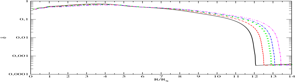
Figure 1: The dependence of disc aspect ratio $\delta$ on radius calculated for the low viscosity run with $\alpha=0.01$. Solid, dashed, dotted, dot-dashed and dot-dot-dashed curves correspond to $t/P_{min}\approx 11,12,13,14,15$, respectively.

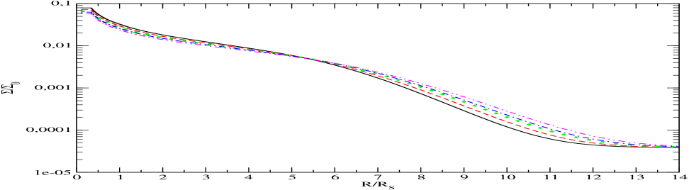
Figure 2: Same as Fig. 1, but for the disc’s surface density expressed in units of its characteristic value $\Sigma_{0}={m/(2\pi R_{S}^{2})}$.

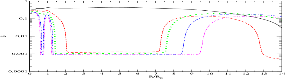
Figure 3: Same as Fig. 1, but at later times. Solid, dashed, dotted, dot-dashed and dot-dot-dashed curves correspond to $t/P_{min}\approx 20,40,60,80,100$, respectively.

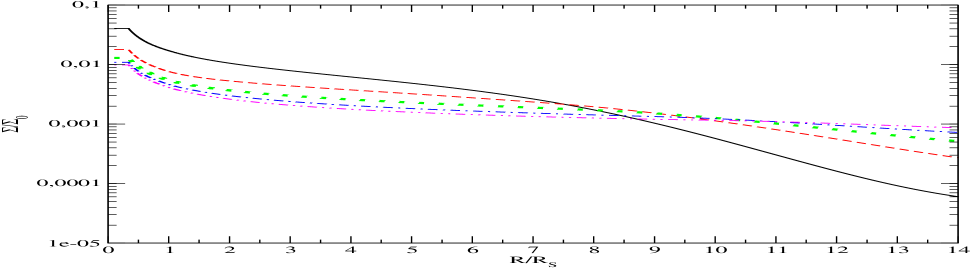
Figure 4: Same as Fig. 3, but for the surface density expressed in units of its characteristic value $\Sigma_{0}={m/(2\pi R_{S}^{2})}$.

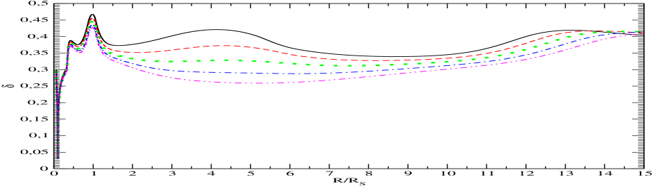
Figure 5: Same as Fig. 1, but for the run with larger $\alpha=0.1$.

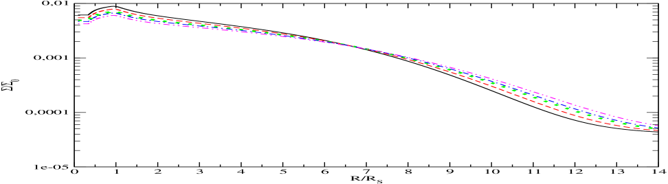
Figure 6: Same as Fig. 5, but for the surface density expressed in units of its characteristic value $\Sigma_{0}={m/(2\pi R_{S}^{2})}$.

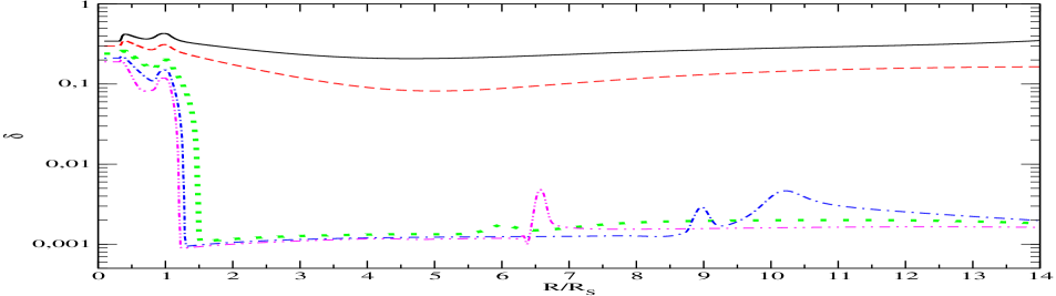
Figure 7: Same as Fig. 3, but for the run with $\alpha=0.1$.

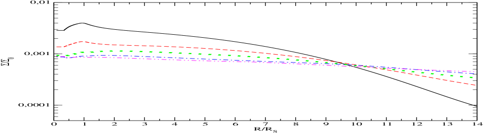
Figure 8: Same as Fig. 7, but for the surface density expressed in units of its characteristic value $\Sigma_{0}={m/(2\pi R_{S}^{2})}$.

For reference we provide some results of our calculations of the background quantities in Figs. 1-8 for cases $\alpha=0.1,$ and $\alpha=0.01.$ Values of $\alpha=0.1$ and $\alpha=0.3$ were considered in Xiang-Gruess et al. (2016). Figs 1-4 illustrate the case with small $\alpha=0.01,$ while Figs. 5-8 correspond to the case with $\alpha=0.1$.

In Figs. 1 and 2 the forms of the disc aspect ratio $\delta$ and surface density $\Sigma$ are shown as functions of $R$ at five, relatively small, values of time, $t/P_{min}\approx 11,12,13,14$ and $15$. We see that while the surface density distributions at these different moments of time are quite similar, and are monotonically decreasing with $R$ and smooth functions of time, the distributions of $\delta$ behave in a more complicated way. They all describe a geometrically thick disc for $R/R_{S}\sim<10$ joined by a transition region in which $\delta$ sharply decreases with $R.$ This joins to a very thin outer disc with $\delta<10^{-3}$. The boundary between the transition region and the thin disc is very sharp having the character of a shock front. It moves outwards with time. We find that the propagation speed of this boundary referred hereafter to as the speed of transition front, $v_{f}$, exceeds the sound speed in the outer disc. The propagation speed may be estimated from the following simple arguments. Namely, it is well known that a characteristic time scale of the development of thermal instability $t_{Th}\sim\alpha^{-1}\Omega^{-1}$. On the other hand, from Fig. 1 it follows that a typical radial extent of the transition front $\Delta R$ is of the order of a typical disc thickness behind the front $\sim 0.1R$. It is expected that $v_{f}\sim\Delta R/t_{th}=0.1\alpha v_{K}=10^{-2}v_{k}$, where $v_{K}=R\Omega$ is Keplerian velocity. This estimate can exceed the sound speed in the outer cold disc and is consistent with our numerical results, which give a value of $v_{f}$ twice as large. The very outermost part of the transition region may thus take on the character of a shock.

Figs. 3 and 4 show the functional forms of $\delta$ and $\Sigma$ at later times $t/P_{min}=20,40,60,80$ and $100.$ One can see in Fig. 3 that at times $>40P_{min}$ the aspect ratio drops to very small values for $2<R/R_{S}<6-7$. A region around $R/R_{S}=1$ always has a large value of $\delta$. This is due to heating of disc material by the stream. Note that there is also a region of large $\delta$ at larger radii, $R/R_{S}>6-9$. This is because outward transport of angular momentum and mass has caused the surface density to significantly increase at the later times relative to its initial value. This results in these regions increasing their optical thickness, heating up and undergoing thermal instability,

As seen from Fig. 4 the functional form of the surface density as a function of radius gets flatter with time.

Results for the case of relatively large $\alpha=0.1$ are illustrated in Figs. 5 and 6. These show the same quantities at the same times as in respectively Figs 1 and 2. However, the plots in Fig. 5 show that contrary to the case of small $\alpha,$ at the early times considered $\delta$ has relatively large values throughout the computational domain with a slight bump at $R/R_{S}\sim 1$ due to heating by the stream. In fact this simulation does exhibit an outward propagating front similar to that seen in Fig. 1. However, it reaches the outer boundary after a time $\sim 2.6$ which is before the earliest time illustrated here (see Xiang-Gruess et al., 2016). Fig. 6 shows that surface density profiles are also close to each other, they all have a maximum at at $R/R_{S}=1$ and smoothly decrease towards larger radii.

Fig. 7 shows that at for times exceeding on the order of $60P_{min}$ $\delta$ drops to small values at radii slightly larger than $R_{S}.$ Note that there are some indications of the propagation of thermal waves of a moderate amplitude at large radii and late times as can be seen from the curves corresponding to $t=80$ and $100$. Fig. 8 shows that as for the case of small $\alpha$ the surface density distribution gets flatter at late times.

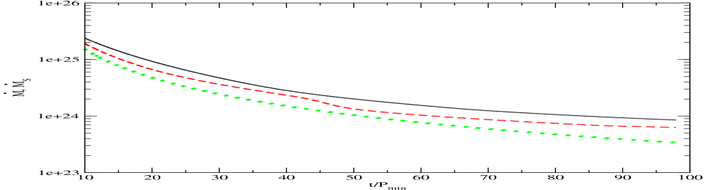
Figure 9: Accretion rates in g/s as functions of time are shown as solid and dashed curve for $\alpha=0.01$ and $\alpha=0.1$, respectively. The dotted curve shows the mass flow in the stream given by equation (3).

Finally, in Fig. 9 we show the dependence of accretion rate, ${\dot{M}},$ determined as the magnitude of the mass inflow rate at the innermost grid point of our computational domain on time in comparison with the stream mass flow rate $\dot{M}_{S}$ given by equation (3), for both $\alpha=0.01$ and $\alpha=0.1$. As seen from this Figure both accretion rates deviate from $\dot{M}_{S}$ at late times taking on larger values, with the curve corresponding to $\alpha=0.01$ showing a larger deviation.

3.2 The governing equations for a twisted tilted disc

The dynamical equations we adopt for the propagation of disc tilt and twist are the same as were used by Morales Teixeira et al. (2014) and Zhuravlev et al. (2014) apart from the fact that we here allow for an isothermal density structure in the vertical direction which takes the form

$$\varrho(R,z,t)=\rho(R,t)\exp{(-z^{2}/(2H^{2}))},$$ (10)

where the mid-plane density $\rho$ and disc semi-thickness $H$ are, in general, functions of radius $R$ and time. The dynamical equations we use can be easily obtained from expressions contained in Zhuravlev & Ivanov (2011), as outlined in appendix A. Here we only discuss their form and some basic properties.

As in previous our work, the $\alpha$ parameter entering our dynamical equations is defined through the relation

$$\nu=\alpha\delta^{2}\sqrt{GMR},$$ (11)

where $\nu$ is the kinematic viscosity defined above. But note that this definition differs from that made through (9) (see below for a reconciliation).

There are, in general, two independent variables that specify the orientation of the disc, the variable ${\cal{W}}$ introduced above and an additional variable ${\cal{B}}$, which describes the deviation of the trajectories of disc particles from circular form due to the presence of the disc tilt and twist (see equation (30). Note that some authors (e.g. Demianski & Ivanov (1997)) use ${\cal{A}}=-{i\over 2}{\cal{B}}$ instead of ${\cal{B}}$.

The dynamical equation for ${\cal{B}}$ has the form

$$\frac{\partial{\cal{B}}}{\partial\tau}=\frac{1}{2}\left\{\left[1+\frac{\kappa^{2}}{(i-\alpha)^{2}\Omega^{2}}\right](i-\alpha)\Omega{\cal{B}}-\left[(i+\alpha)U^{\varphi}\Omega-\frac{3i\alpha}{i-\alpha}K_{1}(U^{\tau})^{2}U^{\varphi}\tilde{\Omega}\right]K_{1}\frac{\partial{\cal{W}}}{\partial R}\right\},$$ (12)

where we use geometrical units, expressing spatial and temporal scales in terms of $GM/c^{2}$ and $GM/c^{3}$, respectively. We define the time expressed in these units as $\tau=tc^{3}/(GM).$ Expressed in these units, $\Omega=R^{-3/2}$ is the angular frequency of a free particle moving on a circular orbit around a non rotating black hole, $\kappa$ is the relativistic epicyclic frequency, and $\tilde{\Omega}$ is another characteristic frequency. Expressions for $\kappa$ and $\tilde{\Omega}$ are given by

$$\kappa=\sqrt{R^{-3}\left(1-\frac{6}{R}\right)},\quad\tilde{\Omega}=\frac{R-3}{R^{2}(R-2)^{1/2}}.$$ (13)

The quantities $U^{\tau}$ and $U^{\varphi}$ represent two components of the four velocity of a free particle moving on a circular orbit around a Schwarzschild black hole and are given by

$$U^{\varphi}=(R-3)^{-1/2},\hskip 5.69054pt{\rm and}\quad U^{\tau}=\left(\frac{R-2}{R-3}\right)^{1/2}.$$ (14)

The metric components of a Schwarzschild black hole in the usual coordinate system are defined by $K_{1}=\sqrt{R-2)/R}$.

The dynamical equation for ${\cal{W}}$ has the form

$$\frac{\partial{\cal{W}}}{\partial\tau}-i\Omega_{\mathrm{LT}}{\cal{W}}+K_{1}^{2}\left\{\frac{U^{r}}{U^{\tau}}+\frac{3}{2}\alpha K_{1}U^{\tau}U^{\varphi}\delta^{2}\right\}\frac{\partial{\cal{W}}}{\partial R}=\\ K_{1}\left(\,2R^{2}U^{\tau}U^{\varphi}\Sigma\,\right)^{-1}\frac{\partial}{\partial R}\left\{\Sigma R^{3}K_{1}\delta^{2}U^{\varphi}\left[\,\,\left(i+\alpha\right){\cal{B}}+\alpha_{1}K_{1}U^{\varphi}\frac{\partial{\cal{W}}}{\partial R}\,\right]\right\}+\dot{\cal{W}}_{S},$$ (15)

where $\dot{\cal{W}}_{S}$ is given by equation (6), in our dimensionless units the Lense-Thirring frequency takes the form

$$\Omega_{LT}=\frac{2a}{R^{3}},$$ (16)

and $U^{r}$ is a component of the four-velocity describing the drift of gas elements in the radial direction due to viscosity. It is given by the expression

$$U^{r}=-3\alpha{(1-{3/R})\over\sqrt{(1-2/R)}(1-6/R)}R^{-1/2}\Sigma^{-1}{\partial\over\partial R}\left\{{\left({(1-{2/R})\over(1-{3/R})}\right)}^{3/2}{\left({H\over R}\right)}^{2}R\Sigma\right\}.$$ (17)

Note that we use a different value of the viscosity parameter, $\alpha_{1}$, in the last term in the brackets on the right hand side of equation (15). As will be discussed below we take $\alpha_{1}$ to be larger than the formally expected value, $\alpha,$ in the vicinity of certain values of $R$ to deal with a specific numerical instability, which is present in the system when $\alpha$ is sufficiently small.

Equations (12) and (15) formally describe the dynamical evolution of the disc tilt and twist in a fully relativistic setting under the assumption that black hole rotation is small, and, accordingly, $|a|\ll 1$. However, these equations can also be used in a situation when $|a|\sim 1$ and scales much larger than the gravitational radius are considered as will be done below. In this context we note that relativistic effects are more significant for the description of the disc tilt and twist than for the background state on account of the importance of small deviations from non relativistic Keplerian motion being able to play an important role in the former case. Accordingly the background quantities $\Sigma$ and $\delta$ entering (12) and (15) are calculated using a non-relativistic numerical code and on a limited computational domain. Also the definitions of $H$ and as noted above, $\alpha,$ in the equations describing background quantities differ slightly. It is easy to see that in order to match definitions of $H$ and $\alpha$ through equations (9) and (8) and, respectively, through equations (10) and (11) we should assume that the values of $H$ and $\alpha$ to be adopted in equations (12) and (15) are slightly less than those used in the equations for the background quantities, through the mappings $H\rightarrow H/\sqrt{2}$ and $\alpha\rightarrow{2\over 3}\alpha$ as will be understood below.

After these adjustments are made we extrapolate numerically obtained values of $\delta$ and $\Sigma$ to smaller radii through a procedure described in Appendix B.1.

In addition we assume that near the marginally stable orbit, the disc is quasi-stationary and is close to the Novikov $\&$ Thorne (1973) solution. As discussed by Novikov $\&$ Thorne (1973) both $\delta$ and $\Sigma$ should be proportional to the function

$$D=1-{\sqrt{6}\over y}-{\sqrt{3}\over 2y}\ln{{(y-\sqrt{3})(3+2\sqrt{2})\over(y+\sqrt{3})}},$$ (18)

where $y=\sqrt{R}$ which vanishes at the marginally stable orbit. Accordingly in addition to the above mentioned extrapolation, we multiply $\delta$ by the factor $D^{3/20}$ and $\Sigma$ by the factor $D^{7/10}$, which are appropriate in the situation where the disc is gas pressure dominated with opacity determined by Thomson scattering. Note that the assumption of gas pressure domination fails at sufficiently early evolution times of our system. Nonetheless we continue to use these factors even in this case since a more appropriate renormalisation of $\delta$ and $\Sigma$ was found to not to influence our results significantly.

3.2.1 The governing equations in the large radius and low viscosity limit

Equation (12) and (15) can be brought into a much simpler form under the assumptions that $R\gg 1$ and $\alpha=O(1/R)\ll 1$. In this limit (12) becomes on expanding each term to leading order in $1/R$

$$\dot{\cal{B}}\equiv\frac{\partial{\cal{B}}}{\partial\tau}=-{i\over 2R^{2}}{\partial\over\partial R}{\cal{W}}-\left(\alpha-{3i\over R}\right)\Omega{\cal{B}}$$ (19)

and (15) gives

$$\dot{\cal{W}}\equiv\frac{\partial{\cal{W}}}{\partial\tau}={\delta^{2}\over 2\xi R}{\partial\over\partial R}\left[\xi R^{2}\left(i{\cal{B}}+\alpha_{1}R^{-1/2}{\partial\over\partial R}{\cal{W}}\right)\right]+i\Omega_{LT}{\cal{W}}+\dot{\cal{W}}_{S},$$ (20)

where $\xi=\Sigma\delta^{2}R^{1/2}.$ The stationary variant of these equations with $\dot{\cal{B}}=\dot{\cal{W}}=0$ was solved in Xiang-Gruess et al. (2016). When $\xi=1$ and $\alpha_{1}=\dot{\cal{W}}_{S}=0$ these equations coincide with those derived in Demianski & Ivanov (1997). As was indicated previously the first term on the right hand side of (19) results from the influence of pressure on the motion of gas particles on nearly circular trajectories in the disc, while the terms in the brackets describe the influence of viscosity and the post Newtonian correction leading to Einstein precession of free particles moving around a black hole.

3.2.2 Local dispersion relation

It is instructive to obtain a dispersion relation derived from equations (19-20). Setting $\dot{\cal{W}}_{S}=0$ and assuming that both dynamical variables $\propto e^{i(\omega\tau+kR)}$ with $kR\gg 1$ so that we may adopt a local perturbation analysis, we find that local perturbations are governed by the dispersion relation

$$\left(\omega-\Omega_{LT}-i\gamma_{1}\right)\left(\omega-{3\Omega/R}-i\alpha\Omega\right)={\delta^{2}\Omega^{2}(kR)^{2}\over 4},$$ (21)

where $\gamma_{1}=(1/2)\alpha_{1}\delta^{2}(kR)^{2}\Omega$.

Sufficiently far from the black hole the contributions of the Lense-Thirring frequency and the post-Newtonian correction, contributed by the second term in the second bracket on the left hand side of (21), can be neglected. In this case, in the low viscosity limit for which $\alpha<\delta,$ the tilt and twist propagate as waves with no dispersion and propagation speed equal to one half of the sound speed, $Re(\omega)\approx\pm(1/2)\delta\Omega kR,$ (see Papaloizou & Lin, 1995) and decay rate approximately equal to $(1/2)(\alpha\Omega+\gamma_{1}).$ From the condition $\gamma_{1}<\alpha\Omega$ we find a condition that the term proportional to $\alpha_{1}$ is unimportant to be

$$\alpha_{1}<{2\alpha\over\delta^{2}(kR)^{2}}.$$ (22)

4 The dynamics of tilt and twist when an outward propagating front separates an inner hot region from an outer cool region

In this Section we discuss the behaviour of the inclination angle $\beta$ as a function of radius $R$ when the background disc model has an outward propagating front that separates an inner hot region of the disc with moderately large aspect ratio from an outer low aspect ratio cool region as illustrated in Fig. 1. In doing this we first discuss a numerical instability that may be present in the calculation of $\beta,$ the physics that drives this and how it can be brought under control.

4.1 A numerical instability arising from the pile up of outward propagating short wavelength bending waves at the transition front with nearly uniform inclination angle at smaller radii

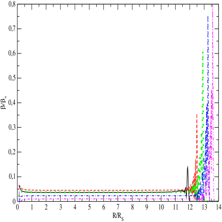
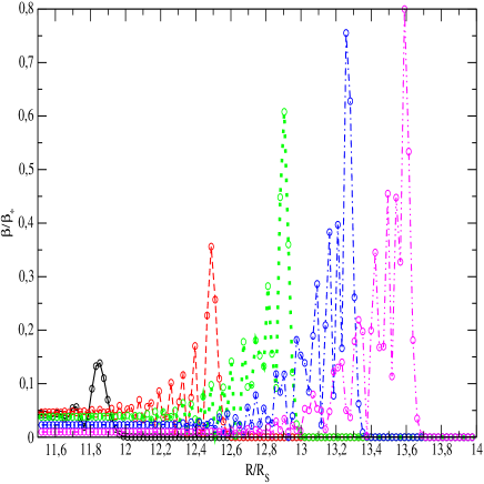
Figure 10: The dependence of the ratio of the disc inclination $\beta$ to the stream inclination $\beta_{*}$ calculated for the $\alpha=0.01$ run at the same moments of time as those corresponding to the curves plotted in Figs. 1 and 2 is shown in the left panel . As for those Figs. solid, dashed, dotted, dot-dashed and dot-dot-dashed curves correspond to $t/P_{min}\approx 11,12,13,14,$ and $15,$ respectively. The region in the neighbourhood of the propagation front is shown in greater detail in the right panel. Symbols indicate the locations of grid points.

In Fig 10 we show the dependence of the inclination angle $\beta$ on radius $R$ calculated in a run with a small value of $\alpha=0.01$, for the same moments of time as shown in Figs 1 and 2. Note that in this run we set $\alpha_{1}=\alpha$ in (15), begin the calculation at $t=10P_{min}$ assuming that the disc is flat and lies in the equatorial plane at that time. Note that because this is a linear response calculation, the calculated value of $\beta$ scales with $\beta_{*}.$ There are two distinctive features seem in the functional forms of the inclination angle. Firstly, at a radii ranging from $R\sim 11-14R_{S},$ with larger radii corresponding to later times, we see very sharp changes of $\beta$ with typical amplitude increasing with time. When $t=11P_{orb}$ $\beta$ has a resolved spike at $R\sim 11.85R_{S}.$, At later times short wavelength oscillations develop. Fig. 10 shows that the wavelength of the oscillations attains the order of grid size, and, therefore, at times larger than approximately $12P_{min}$ our grid is not adequate to resolve the length scales associated with the behaviour of our system. We have checked that when the grid size is reduced there is always a time when the wavelength of the oscillations gets comparable to that size. Also, one can check that, regardless of grid size and type of numerical scheme, residuals in a representation of the law of conservation of angular momentum (see equation C5 in Zhuravlev et al. (2014)) get progressively larger with time and eventually become too large for the computation to be reliable.

There is a simple physical explanation for this behaviour of the system. As we have mentioned above when $\alpha$ is sufficiently small, the twist and tilt propagate with a speed equal to a half that of sound. At any moment of time a maximum of $\beta$ is approximately located at the radius, $R_{f}$, where half of sound speed, $c_{s}$, is equal to the speed of outward moving material in the hot phase which is also close to the propagation speed of the front, $v_{f}.$ Noting that before $t/P_{min}\approx 15,$ $v_{f}$ is approximately constant we can assume that near and interior to $R_{f}$ the sound speed is approximately stationary in the frame moving with $v_{f}$ and such that $c_{s}/2-v_{f}$ is positive. On the other hand the sound speed decreases outwards. Therefore, the propagation speed of bending waves in the moving frame, $c_{s}/2-v_{f}$, becomes zero at $R_{f}$ and bending waves moving outwards from inner radii accumulate there as their wavelengths arbitrarily shorten, the pile up eventually leading to a singularity in the absence of a physical mechanism that allows disturbances induced by the outgoing bending waves to pass through the front. In that case numerical instability occurs. Physically, the manifestation of this singularity would be modified either by taking into account either non-linear terms in $\beta$ or including higher order terms in the expansion in powers of $\delta$ that has has been used in order to obtain equations (12) and (15). The latter approach make the propagation of bending waves dispersive, potentially allowing leakage through the critical point $R=R_{f}$. However, both approaches are technically complex and need to be studied in depth in three dimensions. Here, in order to resolve this difficulty, we artificially increase the coefficient $\alpha_{1}$ in (15) in a region close to $R=R_{f}$. This enables accumulating bending wave action to diffuse away from $R=R_{f}$ at a rate governed by the magnitude of $\alpha_{1}$ thus avoiding the production of singular behaviour. From equation (22) it follows that this term is in fact, of order $\delta^{2}$ with respect to the leading dissipative term $\propto\alpha$, and that making it artificially large doesn’t spoil the dynamics of our system as long as scales much larger than $H$ are considered and $\delta_{f}=\delta(R_{f})$ is not too large. Accordingly we expect our approach to give similar results to any procedure that resolves the issue through diffusive effects limiting the development of small scales near $R=R_{f}.$

Typically, $\delta_{f}\sim 5\cdot 10^{-3}$ (see Fig. 1) and, as seen from (22) when formally considering scales order of $R$ and, accordingly, $k\sim 1/R$ we can introduce very large values of $\alpha_{1}$: $\alpha_{1}\sim<10^{5}\alpha$ without disturbing the dynamics of our system on these scales even without localising its application as indicated below. In our numerical work below we are going to consider

$$\alpha_{1}=\alpha_{1}(R=R_{f})(1+\exp{-{(R-R_{f})^{2}/(4L^{2}_{\alpha_{1}})}}).$$

The spatial scale $L_{\alpha_{1}}$ is chosen to be the maximum of either $H(R_{f})$ or the distance between neighbouring grid points at $R=R_{f}$. This will be done only for the runs with $\alpha=0.01$, which exhibit this type of instability. As will be seen, introducing artificially large $\alpha_{1}$ can indeed regularise the behaviour of our system close to $R=R_{f}$ producing there a spike in $\beta$ with a finite amplitude We check below that making $\alpha_{1}$ ten times larger or smaller practically does not influence our results, apart from making the spike amplitude smaller or larger, respectively.

Another feature concerning functional forms of $\beta$ and $\gamma$ is that they are close to being constant for $R<R_{f}$ during the stage when the front separating the hot phase from the cold phase ahead of it propagates outwards. An explanation for this easily follows from equations (19) and (20). Indeed, let us assume that both ${\cal{B}}$ and ${\cal{W}}$ vary in time on some time scale expressed in dimensionless units, $T_{*},$ and, accordingly, $\dot{\cal{B}}\sim{\cal{B}}/T_{*}$ and $\dot{\cal{W}}\sim{\cal{W}}/T_{*}$. We also assume, as suggested by numerical calculations, that spatial scale of variation of ${\cal{B}}$ is $R$, while the corresponding spatial scale of variation of ${\cal{W}}$, $L$, should be found from (19) and (20). Retaining only the terms containing the highest order spatial derivatives on the right hand sides while neglecting the contribution of the term proportional to $\alpha_{1}$, we get from (19) that $|{\cal{B}}|\sim T_{*}|{\cal{W}}|/(R^{2}L)$, while from (20) we get $|{\cal{W}}|\sim\delta^{2}T_{*}|{\cal{B}}|$. From these two expression we get $L\sim(T_{*}/T_{s})^{2}R$, where $T_{s}=\delta^{-1}\Omega^{-1}$ is a characteristic time for a sound wave to propagate across the region of interest and we recall that $\Omega=R^{-3/2}$ in our dimensionless units. Thus, $L\gg R$ as long as $T_{*}\gg T_{s}$, being the condition that ${\cal{W}}$ should remain approximately constant over a scale $R$ which is satisfied in the inner region of the disc filled by a relatively hot gas. This situation is similar to the known case of sufficiently thick tilted accretion discs in close binary systems (see Larwood et al., 1996).

4.2 An ordinary differential equation giving an approximate description of the time evolution of ${\cal{W}}$ for $R<R_{f}$

That $\cal{W}$ is nearly constant inside $R_{f}$ during the stage of outward propagation of the hot phase allows us to reduce the evolution equations for ${\cal{W}}$ and ${\cal{B}}$ to a single first order equation using equation (20). To do this we multiply both parts of this equation $\xi R/\delta^{2}$ and integrate over a region from the marginally stable orbit to $R_{f}$. The surface terms may be shown to be unimportant and, therefore, we obtain

$$\dot{\cal{W}}_{0}={1\over I_{1}}\left[2ia{G^{2}M^{2}\over c^{3}}I_{2}{\cal{W}}_{0}+{\dot{M}_{S}R_{S}^{1/2}\over 2\pi}({\cal{W}}_{*}-{\cal{W}}_{0})\right],$$ (23)

Here ${\cal{W}}_{0}$ is the value of ${\cal{W}}$ in the inner hot region which is assumed to depend only on time,

$$I_{1}=\int dRR^{3/2}\Sigma,\quad{\rm and}\quad I_{2}=\int dRR^{-3/2}\Sigma,$$ (24)

Here we have used (7), (6) and have temporarily restored physical units. The integration in (24) is formally performed from the radius of the last stable orbit to $R=R_{f}$. The contribution of boundary terms associated with both limits may be shown to be unimportant since the surface density has its maximum near $R_{S}$ and the factor $D^{7/10}$ that scales the surface density vanishes at the last stable orbit ( see the discussion below equation (18)) .

The expression (23), which can be regarded as an ordinary differential equation for ${\cal{W}}_{0},$ reflects the law of conservation of angular momentum for the disc matter with $R<R_{f}.$ This is affected only by the source produced by the stream and the gravito-magnetic torque. We solve this equation for ${\cal{W}}_{0}$ numerically and compare the result with results of solution of the full set (12) and (15) below.

4.3 An approximate treatment of the transition region close to $R_{f}$

Now let us consider the region close to $R_{f}$. In this region we assume that the aspect ratio $\delta$ as well as variables ${\cal{W}}$ and ${\cal{B}}$ are stationary in the frame moving with front propagation speed $v_{f}$. Accordingly the time derivatives in (19) and (20) can be replaced by $-v_{f}\partial/\partial R$ with the consequence that these equations become ordinary differential equations. We introduce a dimensionless variable $y=1-R/R_{f}$ and consider only the region for which $y\ll 1.$ All coefficients in (19) and (20) apart from $\delta$ will be assumed to vary slowly compared to ${\cal{B}}$ and ${\cal{W}}$ so that they can be replaced constants equal to their value evaluated at $R=R_{f}.$ Note that this assumption, made for simplicity, is rather crude since $\Sigma$ has significant variation in this region. In this context we remark that the purpose of this Section is to construct an approximate theory that exhibits the main features of the transition region rather that a precise quantitative representation. In this spirit we also neglect terms proportional to $\Omega{\cal{B}}$ on the right hand side of (19) and last two terms on the right hand side of (20) due to Lense-Thirring precession and that the stream respectively.

Equations (19) and (20) can then be integrated once immediately. The resulting form of (19) can then be used to express ${\cal{B}}$ in terms of ${\cal{W}}$ and the result used in (20) after integration. In this way find that ${\cal{W}}$ satisfies

$$\delta^{2}\alpha_{1}\tilde{v}{d{\cal{W}}\over dy}+\left(\delta^{2}-{\tilde{v}}^{2}\right){\cal{W}}=C_{1}+C_{2}\delta^{2},$$ (25)

where $\tilde{v}=2v_{f}/v_{K}=2\sqrt{R_{f}}v_{f}$ with $v_{K}=R_{f}^{-1/2}$ being the Keplerian speed of circular motion expressed in our dimensionless units and $C_{1}$ and $C_{2}$ are constants of integration. Note that we assume that the front propagates with the sound speed at $R=R_{f}$ so that we have $\tilde{v}=\delta(R_{f})$.

When the term proportional to $\alpha_{1}$ is negligible, as expected significantly inward of the front, we get immediately from (25)

$${\cal{W}}={C_{1}+C_{2}\delta^{2}\over\delta^{2}-{\tilde{v}}^{2}}.$$ (26)

When $\delta\gg\tilde{v}$ the solution (26) must coincide with the solution, ${\cal{W}}_{0},$ given by (23) that is applicable to the interior region. This leads to the requirement that $C_{1}=0$ and $C_{2}={\cal{W}}_{0}$.

An analytic solution of (25) can be found very close to $R_{f}$, by expanding $\delta$ in a Taylor series in $y$ up to the first order and then setting $\delta^{2}-{\tilde{v}}^{2}=2\delta\delta^{\prime}y,$ where the $\prime$ denotes the derivative with respect to $y$ evaluated at $y=0,$ and $\delta^{2}={\tilde{v}}^{2}$ elsewhere in (25) which then gives

$$\alpha_{1}{\tilde{v}}^{2}{d{\cal{W}}\over dy}+2\delta^{\prime}y{\cal{W}}={\tilde{v}}{\cal{W}}_{0}.$$ (27)

A solution to (27) for $y>0,$ can be expressed in terms of the Dawson function
 $Daw(z)=\exp(-z^{2})\int_{0}^{z}dt\exp(t^{2})$. It takes the form

$${\cal{W}}=\frac{1}{\sqrt{{\alpha_{1}\delta^{\prime}}}}\left({\delta\over\tilde{v}}\right)^{2}{\cal{W}}_{0}Daw(z),\quad{\rm with}\quad z=\sqrt{\frac{\delta^{\prime}}{\alpha_{1}{\tilde{v}}^{2}}}y,$$ (28)

where we remark that $\delta^{\prime}>0.$ Note also the factor $(\delta/\tilde{v})^{2}$ inserted in (28). It is close to one near the critical point, but is needed to smoothly match the solution to ${\cal{W}}_{0}$ at smaller radii. In addition we assume that the disc has zero inclination upfront of the critical point which is satisfied by (28) as $D(z=0)=0.$

One can can see that (28) is approximately equal to (26) in the asymptotic limit $z\gg 1$, but with $y\ll 1$ It is possible to obtain an approximate form of ${\cal{W}}$, which is always close to (26) when $z\gg 1$ and always close to (28) when $y\ll 1$. It can be done through redefinition of the variable $z$ through

$$z={1\over 2}{\delta^{2}-{\tilde{v}}^{2}\over\sqrt{\alpha_{1}\delta^{\prime}\tilde{v}^{4}}}.$$ (29)

It is straightforward to see that when $y\ll 1$ $z$ is reduces to the previous definition. That ${\cal{W}}$ given by (28) and (29) reduces to the form (26) follows from the asymptotic form of $D(z)$: $D(z)\approx 1/(2z)$ when $z\gg 1$.

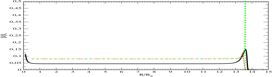
Figure 11: A comparison of the dependence of $\beta$ on $R$ in a numerical calculation (solid curve) and the semi-analytic model developed in this Section (dashed and dotted curves). Parameters and initial conditions of the run are the same as used to obtain the curves shown in Figs 10 except that we now set $\alpha_{1}(R=R_{f})=10^{3}\alpha$.

We compare our semi-analytic model with numerical data in Fig. 11, where we show dependencies of $\beta$ on $R$ at the time $t=15P_{min}.$ in a run with $\alpha=0.01$ The solid curve represents the fully numerical calculation. The dashed curve is obtained using the expressions (28) and (29), while to plot the dotted curve we use the expression (26). In both cases ${\cal{W}}_{0}$ is calculated by solving equation (23) numerically. We see that $\beta_{0}\equiv|{\cal{W}}_{0}|$ overestimates the actual value of $\beta$ by about 60 per cent. Also, although a typical width of the semi-analytic curves is similar to that of numerical one, the maximum value of $\beta$ is roughly 20 percent smaller with a much sharper variation of $\beta$ near the maximum while the total range of $\beta$ is a factor of three smaller. We believe that all of these defects arise through the crudeness of our semi-analytic model and the situation could be improved upon in a more accurate treatment.

5 Numerical results for the evolution of the disc inclination and twist

In this Section we discuss numerical solutions of equations (12) and (15) in detail as well as their comparison with the semi-analytic model developed in the previous Section and the quasi-stationary model developed in Xiang-Gruess et al. (2016). For details of the numerical scheme we used see Appendix B.2. Our numerical runs are distinguished by values of the viscosity parameter, $\alpha$, rotation parameter $a$, initial conditions, which correspond to either a flat disc lying in the equatorial plane or in the plane associated with the stream, and time of the commencement of the simulations. Let us recall that on account of differences in the procedure for reducing the problem to a one dimensional one, in equations (12) and (15) we use values of $\delta$ and $\alpha$ smaller than those used in the equations describing the evolution of background quantities by factors $1/\sqrt{2}$ and $2/3$, respectively. Nonetheless, we label cases corresponding to different $\alpha$ with its value used in the calculation of the background quantities, and only two such values, $\alpha=0.01$ and $\alpha=0.1$ are considered below, we recall that $\alpha=0.1$ and $\alpha=0.3$ were considered in Xiang-Gruess et al. (2016). We consider the cases corresponding to $a=1$, initial time of computation, $t_{in}=10P_{min},$ and initial disc plane coinciding with the black hole equatorial plane and, accordingly, $\beta(t=t_{in})=0$, in more detail than the others. These cases are referred hereafter to as standard.

5.1 The dependence of the inclination angle evaluated at the stream impact position on time

An important quantity, which allows us to make a comparison of our fully numerical results with those obtained using different semi-analytic schemes is the time dependence of the inclination angle $\beta$ evaluated at the stream impact radius $R_{S}$. This quantity also characterises the dependence of typical disc inclinations on time. Let us stress that it is not necessarily the largest value of $\beta$ at a particular time, the latter could be situated at larger or smaller radii depending on the parameters of a particular calculation and time.

5.1.1 The case $\alpha=0.01$

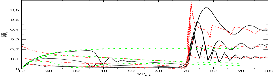
Figure 12: The dependence of inclination angle $\beta$ evaluated at the stream impact position on time. Cases with prograde black hole rotation, $a>0$, are shown for $a=0.25,0.5$ and $1.0.$ The solid curves correspond to the numerical solution of equations (12) and (15), the dashed curves are calculated according to the quasi-static approach described in Xiang-Gruess et al. (2016) and the dotted curves are obtained by numerical solution of equation (23). For curves of a given type, larger values of $\beta$ correspond to smaller values of $|a|.$

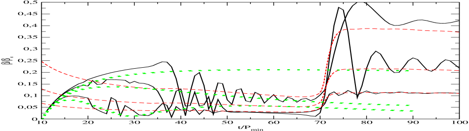
Figure 13: Same as Fig. 12, but for retrograde black hole rotations, $a<0$. When comparing with Fig. 12, corresponding curves are such that $a\rightarrow-a.$

In Figs. 12 and 13 we show the dependence of $\beta(R_{S})$ on time for prograde and retrograde black hole rotation, respectively with absolute values of the rotational parameter $|a|=0.25,0.5$ and $1.0$. Other parameters of the calculations have standard values. As seen from these Figs. values of the inclination get larger when the absolute value of $a$ decreases as expected. A sharp rise of $\beta$ at $t/P_{min}\approx 70$ is associated with the development of thermal instability as explained in Xiang-Gruess et al. (2016). It is also evident from these Figs. that our time dependent model described by equation (23) adequately describes the numerical solutions at relatively early times, $t/P_{min}<15-35$, being significantly better for small, $|a|,$ while the quasi-static solutions are close to the numerical ones at sufficiently late times.

5.1.2 The case $\alpha=0.1$

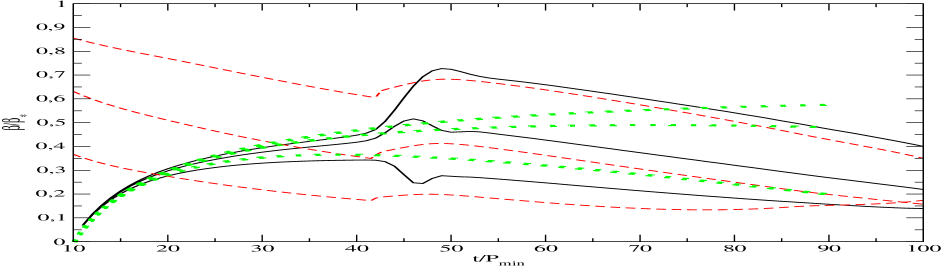
Figure 14: Same as Fig. 12, but for $\alpha=0.1$. Solid curves are obtained numerically, while the dashed ones are calculated in framework of the quasi-static approach. The dotted curve represents calculations based on the solution of equation (23) for the case $\alpha=0.01$. The case of $a>0$ is shown.

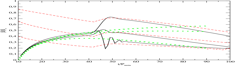
Figure 15: Same as Fig. 14, but for $a<0$.

Figs 14 and 15 are analogous to Fig. 12 and 13, but calculated for larger $\alpha=0.1.$ Since in this case there is no outward propagation of a hot front during the time span of the simulations so that the twist and tilt dynamics is for the most part determined by viscosity rather than effects due to pressure and advection, we do not show results based on equation (23). From these Figs. it follows that inclinations are, in general, larger than those corresponding to the case with $\alpha=0.01$ and that our quasi-static model describes the numerical results quite well at late times.

5.1.3 The effect of changing the initial conditions and varying $\alpha_{1}$

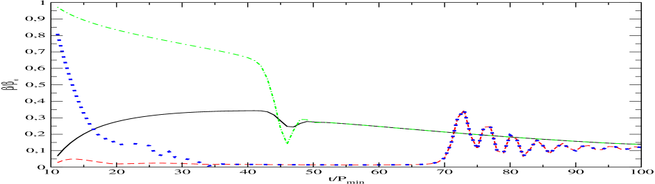
Figure 16: The evolution of $\beta$ at the stream impact position in our standard cases is compared with that obtained by changing the initial value of $\beta$. Solid and dashed curves are for our standard cases with $\alpha=0.1$ and $0.01$, respectively, while dotted and dot dashed curves correspond, respectively, to simulations with the same values of $\alpha$, but set the initial disc inclination to be equal to that of stream,( $\beta(t_{in})=\beta_{*}$). At late times curves corresponding to different values of $\beta_{in}$ but which have the same value of $\alpha$ overlap completely

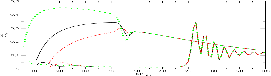
Figure 17: Same as Fig. 17, but now the comparison is between our standard cases and simulations that differ by the choice of commencement time, $t_{in}$. The curves of the same style with larger (smaller) values of $\beta$ at small times correspond to $\alpha=0.1$ ($\alpha=0.01$). Solid curves are for the standard cases, while dashed and dotted curves are calculated for $t_{in}=15P_{min}$ and $t_{in}=5P_{min}$, respectively.

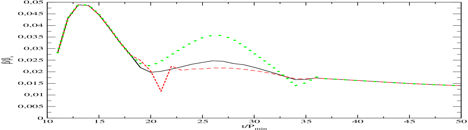
Figure 18: Same as Fig. 17, but now curves of different style correspond to different values of $\alpha_{1}$. Solid, dashed and dotted curves respectively represent cases with the standard $\alpha_{1}=1000\alpha$, $\alpha_{1}=100\alpha$ and $\alpha_{1}=10000\alpha$, respectively. Other parameters have standard values. Note that we show only $t/P_{min}<50$, since the curves completely overlap at later times.

Figs. 16-18 represent results obtained when varying different parameters that specify a simulation. In Fig. 16 we change the initial inclination of the disc to $\beta_{*}.$ In Fig. 17 dashed and dotted curves correspond to the time that the computation was commenced being changed to $t_{in}=15$ and $5P_{min},$ respectively. In 18 we illustrate results obtained by changing the value of $\alpha_{1}(R=R_{f})$ to $100\alpha$ and $10000\alpha$ with respectively dashed and dotted curves. The value of $\alpha$ is $0.01.$ Note that for each of the above cases only one parameter of the problem is varied while keeping the others equal to their standard values.

As seen from these Figs. apart from when the initial value of $\beta$ is changed, variations of different parameters lead to only modest changes of the results with, in particular, no noticeable deviations at later times. The change of initial $\beta$ to $\beta_{*}$ leads to larger values of inclinations at relatively early times, but the curves converge for $t/P_{min}>35$ when $\alpha=0.01$ and for $t/P_{min}>45$ when $\alpha=0.1$.

5.1.4 The dependence of inclination angle on radius at specified moments of time

We now illustrate the dependence of $\beta$ on $R$ at different moments of time. In the low viscosity case we show the curves calculated at ’early’ times, $t/P_{min}=11,12,13,14$ and $15$ corresponding to the situation when the hot phase propagates outwards and profiles of $\beta$ are expected to be nearly uniform at small radii. In addition the form of the inclination is illustrated at ’late’ times $t/P_{min}=40,60,80$ and $100$ when the disc is expected to relax to its quasi-stationary shape. In the high viscosity case only the curves corresponding to the same ’late’ times are shown.

5.1.5 The case $\alpha=0.01$

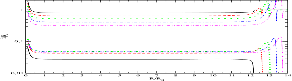
Figure 19: Dependence of $\beta$ on $R$ calculated at relatively early moments of time, when an inner hot region is present in the disc and $\beta$ is nearly constant in this region. Curves of the same type taking on smaller and larger values at a given time correspond to the standard case and the case differing from the standard one by setting $\beta(t_{in})=\beta_{*}$, respectively. Solid, dashed, dotted, dot dashed and dot dot dashed curves are calculated with $t/P_{min}=11,12,13,14$ and $15,$ respectively.

Fig. 19 shows profiles of $\beta$ at the the ’early’ times. Curves of a given type that take on larger values at a given time represent the calculation with $\beta(t_{in})=\beta_{*}$, all other parameters are standard. We see that the disc behaves in the expected manner, with inclinations almost independent of radius inside the front region and a spike in this region. Note that the amplitudes of the spikes are determined by the value of $\alpha_{1}(R=R_{f})$ and so may not be realistic. We recall that this value does not affect the flow elsewhere (see Section 4).

Also note that values of the inclination grow slightly with decreasing radius. This reflects the fact that a low viscosity twisted disc does not align with the black hole equatorial plane when $a>0$, see e.g. Ivanov & Illarionov (1997). We have checked that the prograde case with $a<0$ gives similar curves, but with inclinations tending to alignment at small radii as expected.

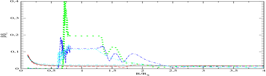
Figure 20: Same as Fig 19, but for the standard case and later moments of time. Solid, dashed, dotted and dot dashed curves correspond to $t/P_{min}=40,60,80$ and $100$, respectively. We also show the results of calculations based on the quasi-static approach by two dot dot dashed lines, with the curve for which $\beta$ is nearly constant for $R/R_{S}\sim>1$ corresponding to $t=40P_{min}$ and the one showing much larger variations of $\beta$ corresponding to $t=100P_{min}$.

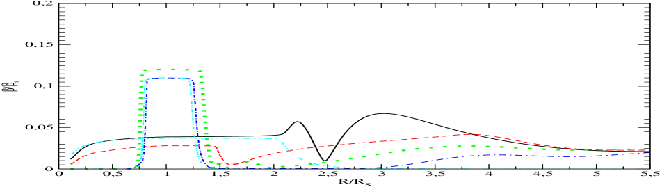
Figure 21: Same as Fig. 20, but for retrograde black hole rotation with $a=-1$. The dot dot dashed curve with larger values of $\beta$ at $R/R_{S}\sim$ is for $t=100P_{min}$ (note that it almost coincides with the corresponding numerical curve), while the other curve of the same type is for $t=40P_{min}$.

Figs 20 and 21 show inclination profiles at ’late’ times. In addition we present two profiles calculated in the framework of our quasi-stationary approach when $t/P_{min}=40$ and $100$ as dot dot dashed curves. At times $t/P_{min}\sim 100$ the the disc inclinations are large only in a region $R\sim R_{S}$ with the result based on the quasi-stationary approximation being very close to the fully numerical one. Note that, as seen in Fig. 20, in the prograde case we have very sharp oscillations of inclination angle at $R/R_{S}\sim 0.75$. This is due to the fact, that a low viscosity twisted disc does not align with the equatorial plane at small radii, instead producing a standing bending wave, (see Ivanov & Illarionov, 1997; Nealon et al., 2015). However, the disc behaviour at close to this radius is, most probably, unphysical, since very sharp changes of $\beta$ are likely to result in Kelvin - Helmholtz like instabilities and possibly an increase in effective viscosity due to non-linear effects associated with their development.

5.1.6 The case $\alpha=0.1$

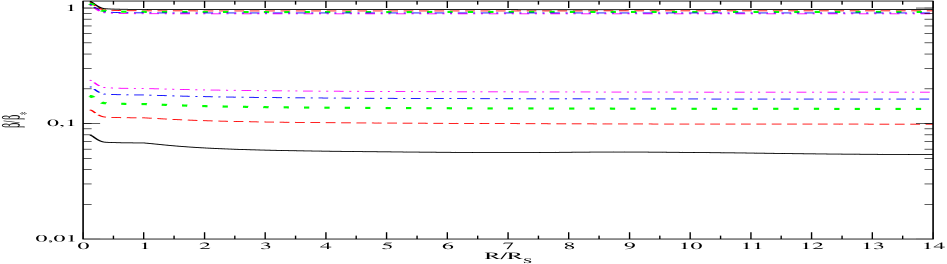
Figure 22: Same as Fig 19, but for $\alpha=0.1$.

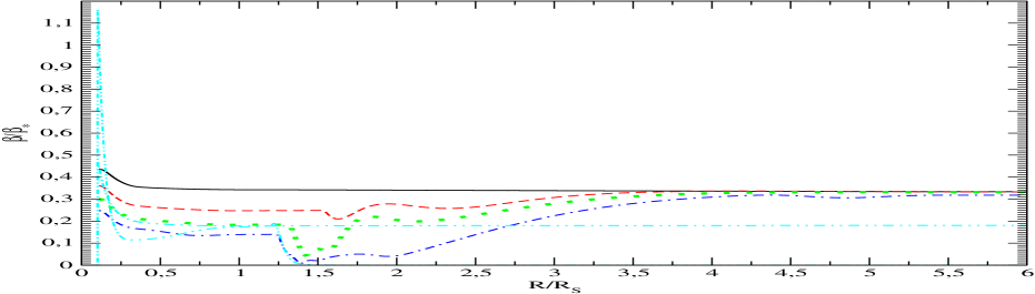
Figure 23: Same as Fig. 20, but for $\alpha=0.1$. Again, the dot dot dashed curve corresponding to $t=40P_{min}$ is nearly flat at sufficiently large radii.

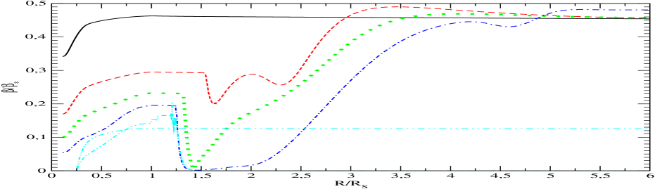
Figure 24: Same as Fig. 23, but for $a=-1$. Again, the nearly flat dot dot dashed curve is calculated in the framework of the quasi-static approach at time $t=40P_{min}$.

Fig. 22 shows profiles of $\beta$ calculated for the ’early’ moments of time $t/P_{min}=11,12,13,14,15$ for the case with $\alpha=0.1,$ $a=1,$ and $t_{in}=10P_{min}$. It shows that similar to the case with $\alpha=0.01$ shown in Fig. 19 the profiles are nearly flat, but, unlike that case there are no spikes in the distributions of $\beta$. Indeed, as seen from Fig. 5 the profiles of $\delta$ are rather uniform at these moments of time for $\alpha=0.1$, so the conditions leading to the formation of a spike are not satisfied.

Figs 23 and 24 show the profiles of $\beta$ calculated at the ’late’ times for the case with $\alpha=0.1$, for prograde and retrograde black hole rotations, respectively. As in the previous case we add two dot dot dashed curves to represent results based on the quasi-stationary approximation for $t/P_{min}=40$ and $100$. Unlike the previous case, even when $t/P_{min}=100$ the quasi-stationary curves are close to the fully numerical ones only at $R/R_{S}\sim 1$. At larger radii inclinations corresponding to the fully numerical calculations are significantly larger.

That difference can be explained by the fact that at larger radii a typical relaxation time to a quasi-stationary configuration, $t_{\nu}\sim(\alpha/\delta^{2})\Omega^{-1}$ (see Papaloizou & Pringle (1983)) is larger than the time elapsed from the beginning of calculations. Indeed, using equation (2) we can express $t_{\nu}$ as $5\cdot 10^{-3}(\alpha/\delta^{2})B_{p}^{3}B_{S}^{-3/2}P_{min}$. Substituting $\alpha=0.1$, $\delta\sim 10^{-3}$, $B_{p}\approx 1.55$ and $B_{S}\approx 0.78$ we get $t_{\nu}\sim 200(R/R_{S})^{3/2}P_{min}$, which indicates that when $t\sim 100P_{min}$ the disc is expected to be far from its stationary state. However, we have checked that when the computational domain s expanded outwards using values of $\delta$ and $\Sigma$ at the outer boundary of the computational grid used to calculate the background quantities, inclinations at large radii drop significantly. Therefore, this effect seems to be sensitive to the size of computational domain and how the outer boundary condition was applied.

5.2 Evolution with time of both inclination and rotation angle

In order to graphically represent time evolution of both Euler angles $\beta$ and $\gamma$ characterising the position of the disc ring with $R=R_{S}$ it is convenient to show time dependencies of $W_{1}=Re({\cal{W}})=\beta\cos\gamma$ and $W_{2}=Im({\cal{W}})=\beta\sin\gamma$ evaluated at $R_{S}$. One can see that $W_{1}$ and $W_{2}$ represent represent a vector perpendicular to the ring angular momentum vector such that its $x$ component is equal to $W_{2}$ and its $y$ component is equal to $-W_{1}$. In addition, they are proportional to the components of a vector lying along the line of intersection of the plane of a local disc ring and the equatorial plane (line of nodes). Thus the time dependence of these components provide information about both the change of inclination and precession of this ring. A uniform precession at constant inclination corresponds to a sinusoidal oscillation. We show $W_{1}$ and $W_{2}$ as functions of time in Figs. 25 and 26 respectively for $\alpha=0.01$ and $0.1.$ These were standard cases with $a=1$ and $t_{in}=10P_{min}$.

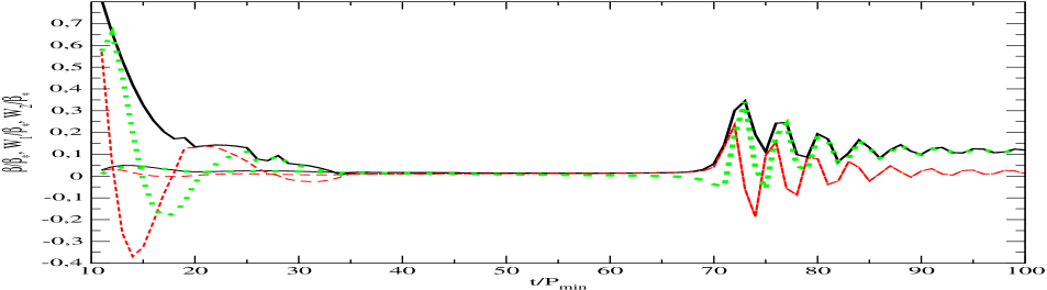
Figure 25: Solid, dashed and dotted line show the evolution of $\beta$, $Re({\cal{W}})$, $Im({\cal{W}})$ evaluated at the stream impact position for our standard case with $\alpha=0.01$, $a=1$ and $t_{in}=10P_{min}$. Curves having larger (smaller ) values of arguments at sufficiently small times correspond to the initial disc configuration being aligned with the stream orbital plane (black hole equatorial plane). These curves become overlapping at large times.

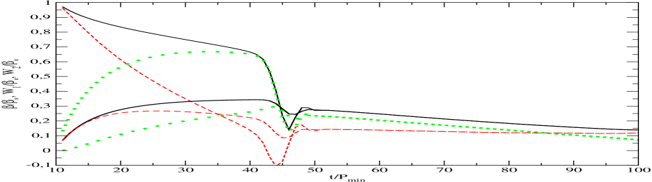
Figure 26: Same as Fig. 25, but for $\alpha=0.1$.

As seen from these Figures, during the early stage of evolution, when distributions of $\beta$ with $R$ are nearly flat the ring accomplishes only one precession period in the case of $\alpha=0.01$ and only a quarter of that in case of $\alpha=0.1$. Precession is also accompanied by a strong evolution of the ring’s inclination due to the influence of the stream. That means that for our parameters, the purely precessional model of disc evolution considered in Stone & Loeb (2012) and Franchini et al. (2016) is not applicable. Note, however, that this model could be more appropriate for smaller values of $R_{S}$ leading to a stronger Lense-Thirring precession.

6 Summary and conclusions

In this Paper we consider the evolution of geometrical form of a disc formed after a tidal disruption event due to impact of material of the stream of gas, which arises from tidally disrupted star. Angular momentum provided by the stream is not, in general, aligned with angular momentum of black hole, so the stream tends to ’push’ the disc away from equatorial way, naturally leading to its twisted geometrical configuration.

We solve time dependent twisted disc equations numerically, for two values of viscosity parameter $\alpha=0.01$ and $0.1$, black hole mass $10^{6}M_{\odot}$ and various values of its rotational parameter $a$ in the linear regime. We find that at relatively late times $t~{}>50P_{min},$ with $P_{min}$ being the minimum return time of gas in the stream to periastron after the disruption of the star, configurations of the twisted disc are close to those obtained in framework of a quasi-stationary approach in which the background quantities are held constant in time while the inclination and twist are allowed to attain a steady state. This approach was adopted in Xiang-Gruess et al. (2016).

6.1 Evolution of the twisted disc after tidal disruption

However, at ’early’ times $t~{}<30P_{min}$ we found that disc shape is far from being quasi-stationary. At these times, inner parts of the disc are geometrically rather thick, with relative thickness $\delta$ exceeding viscosity parameter $\alpha$. As was suggested elsewhere (see, e.g. Stone & Loeb, 2012) this leads to disc’s inclination angle $\beta$ being nearly independent of radius in this region. However, unlike previous studies in Section 5.2 we find that the evolution of disc’s geometrical shape is not simply precessional, since it is determined by both Lense-Thirring torque and the torque arising from the stream. Both inclination angle $\beta$ and precession angle $\gamma$ evolve on a similar time scale and for our simulations with stream impact radius $R_{S}$ equal to $9R_{T}/7,$ with $R_{T}$ being the tidal disruption radius, it took less than one precessional period for this stage to be completed. Note, however, that this would be different for different parameters of the problem, for example reducing $R_{S}$ would make the Lense-Thirring torque stronger, thus speeding up precession. We propose a simple semi-analytic model for this stage in Section 4.2 ( and see equation (23)) , which is based on law of conservation of angular momentum and can be used without having to solve the twisted disc equations. It is enough to know the evolution of the background quantities $\delta$ and $\Sigma$ with time and it allows inclination changes and the amount of precession to be estimated. The duration of this stage is determined by the time needed for the disc to cool down significantly at $R\sim R_{S}$ at which point $\delta$ becomes small on this scale.

6.2 Outward propagating transition front

For the case with $\alpha=0.01,$ in Section 4 we found that during the early stage of evolution, the disc exhibits singular behaviour of its inclination angle. There is an outward propagating transition front that separates an inner hot region from an outer cooler region which constitutes a pre-existing low surface density disc that is coplanar with the black hole equatorial plane. The transition radius $R_{crit}$ eventually extends to $\sim 13R_{S}$. At radii smaller than $R_{crit}$ $\beta$ is nearly uniform, at large radii it is close to zero, while in a narrow region close to $R_{crit}$ there is a sharp growth of $\beta$ leading to formation of a spike in its profile.

When the numerical scheme is not regularised formation of this spike eventually leads to a numerical instability. We regularised our equations by adding additional dissipation in this region parametrising by a value of the coefficient $\alpha_{1}$ at the transition front which is chosen to be $1000\alpha$ for most simulations. We checked that the enhancement of $\alpha_{1}$ changed only the spike amplitude significantly, leaving the solutions outside the region of the spike practically unchanged. Physically, formation of this spike is related to the outward propagation of transition front that separates hot and cold regions. In a low viscosity disc tilt and twist propagate as a bending wave with speed equal to half the sound speed. At the point where the speed of bending waves becomes equal to the propagation speed of the front wave action accumulates leading to singularity and numerical instability. In Section 4.3 we formulated a simple analytic theory of distribution of $\beta$ in this region and checked that it is confirmed by numerical simulations.

A question arises as to what is the physical mechanism that limits the spike amplitude. One possibility is the action of non-linear effects. In this case it’s possible to speculate that the spike’s amplitude could attain values of order unity, $\beta\sim 1$, although various instabilities (see e.g. Ferreira & Ogilvie, 2008, 2009; Ogilvie $\&$ Latter, 2013a, b) could significantly limit its amplitude. If the spike has large amplitude, the disc may take on a broken structure of the type postulated by e.g. Nealon et al. (2016), which could produce significant observational effects through intercepting radiation from the central source. Another possibility would be to equations for the disc tilt and inclination to consider terms of higher order in in $\delta$. Both these possibilities deserve a future study.

6.3 Inclination of the disc at the stream impact radius

In Section 5.1 we calculated the time dependence of the disc inclination at the stream impact radius for different $\alpha$, $a$ and initial conditions. Similar to what was found using the quasi-stationary approach we found that the disc inclination could be large, being of the order $0.1-0.5\beta_{*}$, where $\beta_{*}$ is the inclination of the orbital plane of the stream, for $|a|=1$. For smaller black hole rotation the inclination angle is even larger. The inclination angle attains its largest values as a function of time during the transition from an advective to radiative phase occurring when $t\sim 50-70P_{min}$. Therefore, observations of TDEs during this time could shed light on physical conditions during this transition, including whether the thermal instability operates during this time.

6.4 Discussion

That the disc inclination angle could be large and is a non-trivial function of time and radius could have profound implications on time behaviour of disc’s luminosity and other effects associated with TDEs. Clearly, disc’s luminosity will be modulated by the changing geometrical shape, which would allow us, in, principal, to test different models of the accretion process and provide information on black hole mass and angular momentum. Moreover, it was suggested recently that when a sufficiently thick disc is inclined with respect to the equatorial plane as expected at the ’early’ evolution times, it produces a jet directed perpendicular to the disc plane, see Liska et al (2018). Therefore, the evolution of the geometrical form of the disc may also lead to evolution of the jet luminosity. The issue of the observational appearance of such discs is to be considered in future publications.

Appendix A An outline of the derivation of the governing equation for twisted disc dynamics

In order to derive the relativistic twist equations appropriate for our model, we start from equations (46-48) of Zhuravlev & Ivanov (2011) and consider the case of a vertically isothermal disc with gas density depending on vertical coordinate according to equation (10) where $z$ is understood as a proper distance from the equatorial plane of the twisted disc.

Using their equations (46) and (47) one may derive an equation describing the evolution of the radial velocity perturbation, $v^{r}$, induced by the disc twist and warp. In disc with density distribution given by (10) $v^{r}$ can be represented by the complex state variable ${\cal{B}}=B_{2}+{\rm i}B_{1}$, which we introduce here using the following representation

$$v^{r}=z(B_{1}\sin\varphi+B_{2}\cos\varphi).$$ (30)

The derivation of the equation for ${\cal{B}}$ follows the same procedure as that given in Section 3.3 of Zhuravlev & Ivanov (2011), see their final equation (60), with a remark that here we use the Schwarzschild radial coordinate and the proper vertical coordinate rather than the so-called isotropic radial coordinate, $R_{iso}$, and a similar vertical coordinate, related to $R$ and $z$ through

$$R=K_{2}R_{iso},\quad z=K_{2}z_{iso},$$ (31)

where $K_{2}=(1+1/(2R_{iso}))^{2}$ that was used by Zhuravlev & Ivanov (2011) . Taking this into account, as well as the expression for $r\varphi-$component of the stress tensor of the background flow

$$T^{r\varphi}=\frac{3}{2}\nu\rho K_{1}(U^{\tau})^{2}\frac{U^{\varphi}}{R},$$ (32)

where $\nu$ is given by equation (11), we obtain a equation (12).

The dynamical equation (15) for ${\cal{W}}$ follows from equation (48) of Zhuravlev & Ivanov (2011) after making use of the relations (31), the definition of $\Sigma$ as well as the density distribution (10) together with the explicit form of $T^{r\varphi}$, where $\nu$ is given by equation (11). Note that $\Sigma=K_{2}\Sigma_{ZI}$, where $\Sigma_{ZI}$ is the surface density used in equation (48) of Zhuravlev & Ivanov (2011).

Appendix B Details of the numerical procedure for solving the governing equations

B.1 Extrapolation of dynamical variables to smaller radii

Our inner boundary conditions are set at the radius of the marginally stable orbit of a non-rotating black hole, $R_{ms}=6GM/c^{2}$, where our equations governing the dynamics are formally singular. From these it follows that in order to have regular solutions we must require $\partial{\cal{W}}/\partial R={\cal{B}}=0$ at that location. In order to extend the computational domain used to calculate the background quantities to include the marginally stable orbit we need to make some assumptions about the behaviour of the state variables at small radii. We assume that $\Sigma$ and $\delta$ correspond to a Novikov-Thorne solution near $R=R_{ms}$, which is smoothly matched to the exterior numerical solution through an intermediate matching region. Details of our matching procedure are given below.

Let $R_{i}$ be the inner boundary of the background solution obtained numerically using the Newtonian numerical model, which prescribes values of $\delta_{num}$ and $\Sigma_{num}$ as functions of $R$ and $t.$ As discussed in the main text we multiply $\delta_{num}$ and $\Sigma_{num}$ by factors $D(R)^{3/20}$ and $D(R)^{7/10}$, respectively, where the function $D(R)$ is defined through equation (18) to obtain background quantities $\delta(t,R)$ and $\Sigma(t,R)$ that are used in equations (12) and (15). This procedure is needed in order to match to a quasi-stationary, formally thin, relativistic disc, which must have a fixed value of specific angular momentum at $R=R_{ms}.$

We assume that starting from some $R_{NT}<R_{i}$ the disc is represented by a Novikov-Thorne analytic solution with $\delta=\delta_{NT}D^{3/20}$, where $\delta_{NT}$ is a constant. Further, in an intermediate domain $R_{NT}<R<R_{i}$ we specify

$$\delta_{im}=\delta_{i}+\delta^{\prime}_{i}(R-R_{i})+C_{\delta}(R-R_{i})^{2}$$ (33)

where $\delta_{im}$ is the aspect ratio in the intermediate domain and

$$\Sigma_{im}=\Sigma_{i}+\Sigma^{\prime}_{i}(R-R_{i})+C_{\Sigma}(R-R_{i})^{2}$$ (34)

where $\Sigma_{im}$ is the surface density there. The quantities $\delta^{\prime}_{i}$ and $\Sigma^{\prime}_{i}$ are, respectively, the derivatives of $\delta_{im}$ and $\Sigma_{im}$ found from the numerical solution at $R=R_{i}$.

The unknown coefficients $C_{\delta}$ and $C_{\Sigma}$ are determined by the requirement that the intermediate solution specified by (33-34) matches smoothly to the Novikov-Thorne solution at $R=R_{NT}.$ We define $\Delta\equiv R_{i}-R_{NT}$. In order to match smoothly at $R=R_{NT}$ we require that

$$\frac{d\delta_{im}}{dR}\Biggr{|}_{R=R_{i}}=\frac{d\delta_{NT}}{dR}\Biggr{|}_{R=R_{NT}}=0,$$

This requires that that $C_{\delta}=\delta^{\prime}_{i}/(2\Delta)$. Consequently we have

$$\delta_{NT}=\delta_{i}+\delta^{\prime}_{i}(R_{NT}-R_{i})+\frac{\delta^{\prime}_{i}}{2\Delta}(R_{NT}-R_{i})^{2}.$$

Under the assumption that the turbulent kinematic viscosity coefficient is parametrised via $\alpha$ as given by equation (11), the Novikov-Thorne solution yields the following form of surface density (see equation (36) of Zhuravlev & Ivanov, 2011)

$$\Sigma_{NT}=\frac{\dot{M}}{3\pi\alpha}\frac{D(R)}{K_{1}^{3}U^{\tau}(U^{\varphi})^{2}R^{3/2}\delta_{NT}^{2}},$$ (35)

where $U^{\tau}$ and $U^{\varphi}$ are given by equation (14) and $D(R)$ is given by equation (18)
and $K_{1}=\sqrt{1-2/R}.$ Note that equation (35) may be expressed as

$$\Sigma_{NT}=\frac{\dot{M}}{\delta_{NT}^{2}}F(R),$$ (36)

where $F(R)$ is a known function of $R$.

Matching $\Sigma$ given by equation (34) in the intermediate domain to $\Sigma_{NT}$ at $R=R_{NT}$ requires that

$$\Sigma_{im}(R_{NT})=\Sigma_{NT}(R_{NT})$$ (37)

and matching derivatives requires that

$$\frac{d\Sigma_{im}}{dR}\Biggr{|}_{R=R_{NT}}=\frac{d\Sigma_{NT}}{dR}\Biggr{|}_{R=R_{NT}}$$ (38)

These conditions require that

$$C_{\Sigma}=\frac{\Sigma^{\prime}_{i}/F^{\prime}+\Delta\Sigma^{\prime}_{i}/F-\Sigma_{i}/F}{\Delta^{2}/F+2\Delta/F^{\prime}},$$ (39)

where $F$ and its derivative, $F^{\prime}\equiv dF/dR$, are evaluated at $R=R_{NT}$.

Thus, the disc aspect ratio and the surface density are given by the numerical solution for $R>R_{i}$, by the intermediate solution (33-34) for $R_{i}>R>R_{NT}$ and by the Novikov-Thorne solution (35) with constant $\delta=\delta_{NT}$ for $R<R_{NT}$. For all computations we set $R_{NT}/R_{i}=0.85$ and it has been checked that solutions of the twist equations are insensitive to this choice.

B.2 An implicit grid based scheme

In order to construct the numerical scheme we adopted, let us rewrite equations (12) and (15) in the form

$$\dot{\cal{B}}={\rm i}{\cal{O}}{\cal{B}}+{\cal{F}}{\cal{W}}^{\prime},$$ (40)

$$\dot{\cal{W}}={\rm i}\Omega_{LT}{\cal{W}}+G{\cal{W}}^{\prime}+C({\cal{D}}{\cal{B}}+E{\cal{W}}^{\prime})^{\prime}+\dot{\cal{W}}_{S},$$ (41)

where we represent the source term (6) as a combination of two factors

$${\dot{\cal{W}}}_{S}\equiv{\tilde{\dot{\cal{W}}}}_{S}-{\bar{\dot{W}}}_{S}{\cal{W}},$$

where ${\tilde{\dot{\cal{W}}}}_{S}$ and ${\bar{\dot{W}}}_{S}$ can be easily read off from (6) and ${\cal{O}},{\cal{F}},{\cal{D}}$ and $G,C,E$ are known, respectively, complex and real functions of time and radial coordinate, while the time and the spatial partial derivatives are denoted by dot and prime, respectively.

Let us set up a uniform spatial grid in the variable $x\equiv\sqrt{R}$, i.e. $x_{j}=\sqrt{6}+\delta x+j\Delta x$, where $j=0,1,2,..N$ specifies the spatial node number, $\Delta x$ is the step length and $\delta x$ is the grid offset which is used to avoid the singularity occurring in the coefficients of our equations at the last stable orbit occurring at $x=\sqrt{R}=\sqrt{6}.$ We recall that in setting up these coordinates spatial and temporal scales are expressed in terms of $GM/c^{2}$ and $GM/c^{3}$, respectively. The total number of grid points is $N=1.$ We denote the time step by $\Delta\tau$. The $n_{th}$ time slice is defined to be at time $\tau_{n}=\tau_{n-1}+\Delta\tau.$ The radial extent of the computational domain is $N\Delta x.$ It is assumed that the numerical approximations to the time and spatial derivative of some quantity $A$ are centered at the times $\tau_{n+1/2}=(\tau_{n}+\tau_{n+1})/2$ and at the coordinates $x_{j}$ and are given by the following expressions:

$$(\dot{A})^{n+1/2}_{j}=\frac{A^{n+1}_{j}-A^{n}_{j}}{\Delta\tau},$$ (42)

$$(A^{\prime})^{n+1/2}_{j}=\frac{A^{n+1}_{j+1}+A^{n}_{j+1}-A^{n+1}_{j-1}-A^{n}_{j-1}}{4\Delta x}.$$ (43)

while the quantity itself is given by

$$A^{n+1/2}_{j}=\frac{A^{n+1}_{j}+A^{n}_{j}}{2}.$$ (44)

By $A$ we indicate any of the variables entering the twist equations except the term $(E{\cal{W}}^{\prime})^{\prime}$ which is approximated according to

$$((E{\cal{W}}^{\prime})^{\prime})^{n+1/2}_{j}=\frac{(E{\cal{W}}^{\prime})^{n+1/2}_{j+1/2}-(E{\cal{W}}^{\prime})^{n+1/2}_{j-1/2}}{\Delta x},$$ (45)

where

$$(E{\cal{W}}^{\prime})^{n+1/2}_{j+1/2}=E^{n+1/2}_{j+1/2}\,\frac{{\cal{W}}^{n+1}_{j+1}+{\cal{W}}^{n}_{j+1}-{\cal{W}}^{n+1}_{j}-{\cal{W}}^{n}_{j}}{2\Delta x}$$ (46)

and

$$(E{\cal{W}}^{\prime})^{n+1/2}_{j-1/2}=E^{n+1/2}_{j-1/2}\,\frac{{\cal{W}}^{n+1}_{j}+{\cal{W}}^{n}_{j}-{\cal{W}}^{n+1}_{j-1}-{\cal{W}}^{n}_{j-1}}{2\Delta x}$$ (47)

with

$$E^{n+1/2}_{j\pm 1/2}=\frac{E^{n+1/2}_{j}+E^{n+1/2}_{j\pm 1}}{2},$$ (48)

From the numerical representation of (40) and (41) made with the help of (42-48) we obtain $N-1$ linear inhomogeneous algebraic equations for the state vector

$${\bf q}\equiv[{\cal{B}}^{n+1}_{0},\,{\cal{W}}^{n+1}_{0},\,...,\,{\cal{B}}^{n+1}_{j},\,{\cal{W}}^{n+1}_{j},\,...,\,{\cal{B}}^{n+1}_{N},\,{\cal{W}}^{n+1}_{N}]^{\dagger}$$ (49)

relating the variables at the next slice, $n+1,$ to those at the slice $n.$ These can be represented by the matrix equation

$${\bf M}{\bf q}={\bf B}.$$ (50)

In equation (50) the non-zero elements of ${\bf M}$ are given by

$${\bf M}_{2j-1}^{2j}=\frac{\Delta\tau}{4\Delta x}{\cal{F}}^{n+1/2}_{j},$$

$${\bf M}_{2j}^{2j}=1-\frac{{\rm i}\Delta\tau}{2}{\cal{O}}^{n+1}_{j},$$

$${\bf M}_{2j+3}^{2j}=-\frac{\Delta\tau}{4\Delta x}{\cal{F}}^{n+1/2}_{j},$$

$${\bf M}_{2j-2}^{2j+1}=\frac{\Delta\tau}{4\Delta x}C^{n+1/2}_{j}{\cal{D}}^{n+1}_{j-1},$$

$${\bf M}_{2j-1}^{2j+1}=\frac{\Delta\tau}{4\Delta x}G^{n+1/2}_{j}-\frac{\Delta\tau}{2\Delta x^{2}}C^{n+1/2}_{j}E^{n+1/2}_{j-1/2},$$ (51)

$${\bf M}_{2j+1}^{2j+1}=1-\frac{{\rm i}\Delta\tau}{2}(\Omega_{LT})^{n+1}_{j}+\frac{\Delta\tau}{2\Delta x^{2}}C^{n+1/2}_{j}(E^{n+1/2}_{j+1/2}+E^{n+1/2}_{j-1/2})+\frac{({\bar{\dot{W}}}_{S})^{n+1}_{j}}{2}\Delta\tau,$$

$${\bf M}_{2j+2}^{2j+1}=-\frac{\Delta\tau}{4\Delta x}C^{n+1/2}_{j}{\cal{D}}^{n+1}_{j+1},$$

$${\bf M}_{2j+3}^{2j+1}=-\frac{\Delta\tau}{4\Delta x}G^{n+1/2}_{j}-\frac{\Delta\tau}{2\Delta x^{2}}C^{n+1/2}_{j}E^{n+1/2}_{j+1/2},$$

while the non-zero elements of ${\bf B}$ are explicitly

$${\bf B}^{2j}={\cal{B}}^{n}_{j}\left(1+\frac{{\rm i}\Delta\tau}{2}\Omega^{n}_{j}\right)+\frac{\Delta t}{4\Delta x}F^{n+1/2}_{j}({\cal{W}}^{n}_{j+1}-{\cal{W}}^{n}_{j-1}),$$

$${\bf B}^{2j+1}={\cal{W}}^{n}_{j}\left(1+\frac{{\rm i}\Delta\tau}{2}(\Omega_{LT})^{n}_{j}\right)+\frac{\Delta\tau}{4\Delta x}G^{n+1/2}_{j}({\cal{W}}^{n}_{j+1}-{\cal{W}}^{n}_{j-1})+$$

$$\frac{\Delta\tau}{4\Delta x}C^{n+1/2}_{j}({\cal{D}}^{n}_{j+1}{\cal{B}}^{n}_{j+1}-{\cal{D}}^{n}_{j-1}{\cal{B}}^{n}_{j-1})+\frac{\Delta\tau}{2\Delta x^{2}}C^{n+1/2}_{j}(E^{n+1/2}_{j+1/2}({\cal{W}}^{n}_{j+1}-{\cal{W}}^{n}_{j})$$

$$-E^{n+1/2}_{j-1/2}({\cal{W}}^{n}_{j}-{\cal{W}}^{n}_{j-1}))+({\tilde{\dot{\cal{W}}}}_{S})^{n+1/2}_{j}\Delta\tau-\frac{({\bar{\dot{W}}}_{S})^{n}_{j}{\cal{W}}^{n}_{j}}{2}\Delta\tau$$ (52)

In the expressions (B.2) and (B.2) it is implied that the subscripts and the superscripts of elements of ${\bf M}$ and ${\bf B}$ denote the columns and the row numbers, respectively, with $j$ taking on values from $1$ to $N-1$.

Equation (50) must be completed by representations of the boundary conditions. The latter are the same as in Zhuravlev et al. (2014), explicitly

$${\cal{W}}^{\prime}=0\quad{\rm and}\quad{\cal{B}}=0$$ (53)

at $x=\sqrt{6}+\delta x$ and $x=\sqrt{6}+\delta x+N\Delta x$. This yields the additional conditions

$${\cal{W}}^{n+1}_{0}={\cal{W}}^{n+1}_{1},\quad{\cal{B}}^{n+1}_{0}=0\quad{\rm together\quad with}\hskip 5.69054pt{\cal{W}}^{n+1}_{N}={\cal{W}}^{n+1}_{N-1}\quad{\rm and}\quad{\cal{B}}^{n+1}_{N}=0.$$

Incorporating these conditions in the system (50) leads to additional non-zero elements of ${\bf M}$:

$${\bf M}_{0}^{0}=1,\quad{\bf M}_{1}^{1}=1,\quad{\bf M}_{3}^{1}=-1,\quad{\bf M}_{2N}^{2N}=1,\quad{\bf M}_{2N-1}^{2N+1}=-1\quad{\rm and}\quad{\bf M}_{2N+1}^{2N+1}=1.$$ (54)

The system is solved numerically using the Gaussian elimination method adapted for almost diagonal matrices. In addition the convergence of the solution is checked by making sure that an angular momentum conservation law, which is derived from equation (41) multiplying it by $C^{-1}$ and subsequently integrating over the spatial domain, is satisfied.

References

- Abramowicz et al. (1988) Abramowicz M. A., Czerny B., Lasota J. P., Szuszkiewicz E., 1988, ApJ, 332, 646
- Bonnerot et al. (2016) Bonnerot C., Rossi E. M., Lodato G., Price D. J., 2016, MNRAS, 455, 2253
- Carter & Luminet (1983) Carter B. & Luminet J.-P., 1983, AA, 121, 97
- Carter & Luminet (1985) Carter B. & Luminet J. P., 1985, MNRAS, 212, 23
- Demianski & Ivanov (1997) Demianski M. & Ivanov P. B., 1997, A&A, 324, 829
- Ferreira & Ogilvie (2008) Ferreira B. T. & Ogilvie G. I., 2008, MNRAS, 386, 2297
- Ferreira & Ogilvie (2009) Ferreira, B. T. & Ogilvie, G. I., 2009, MNRAS, 392, 428
- Franchini et al. (2016) Franchini A., Lodato G., Facchini S., 2016, MNRAS, 455, 1946
- Guillochon & Ramirez-Ruiz (2013) Guillochon J. & Ramirez-Ruiz E., 2013, ApJ, 767, 25
- Guillochon & Ramirez-Ruiz (2015) Guillochon J. & Ramirez-Ruiz E., 2015, ApJ, 809, 166
- Hayasaki et al. (2013) Hayasaki K., Stone N., Loeb A., 2013, 434, 909
- Hills (1975) Hills J. G., 1975, Nature, 254, 295
- Ivanov & Illarionov (1997) Ivanov P. B. & Illarionov A. F., 1997, MNRAS, 285, 394
- Ivanov & Novikov (2001) Ivanov P. B. & Novikov I. D., 2001, ApJ, 549, 467
- Ivanov et al. (2003) Ivanov P. B., Chernyakova M. A., Novikov I. D., 2003, MNRAS, 338, 147
- Ivanov & Chernyakova (2006) Ivanov P. B. & Chernyakova M. A., 2006, AA, 448, 843
- Khokhlov et al. (1993b) Khokhlov A., Novikov I. D., Pethick C. J., 1993, ApJ, 418, 181,
- Komossa (2015) Komossa S., 2015, Journal of High Energy Astrophysics, 7, 148
- Lacy et al. (1982) Lacy J. H., Townes C. H., Hollenbach D. J., 1982, ApJ, 262, 120L
- Larwood et al. (1996) Larwood, J. D., Nelson, R. P., Papaloizou, J. C. B., Terquem, C., 1996, MNRAS, 282, 597
- Liska et al (2018) Liska, M., Hesp, C., Tchekhovskoy, A., Ingram, A., van der Klis, M., Markoff, S., 2018, 474, L81
- Lodato et al. (2009) Lodato G., King A. R., Pringle J. E., 2009, MNRAS, 392, 332
- Mashhoon (2003) Mashhoon, B.,“The Measurement of Gravitomagnetism: A Challenging Enterprise”, 2003, edited by L. Iorio (Nova Science, New York, 2007), pp. 29-39, arXiv:gr-qc/031103
- Morales Teixeira et al. (2014) Morales Teixeira D., Fragile P. C., Zhuravlev V. V., Ivanov P. B., 2014, ApJ, 796, 103
- Nealon et al. (2015) Nealon, R., Price D. J., Nixon C. J., MNRAS, 2015, 448, 1526
- Nealon et al. (2016) Nealon, R., Nixon C. J., Price D., King, A., MNRAS, 2016, 455, L62
- Nixon (2015) Nixon, C. J., MNRAS, 2015, 450, 2459
- Novikov Thorne (1973) Novikov, I. D., Thorne, K. S., Black holes (Les astres occlus), p. 343-450. Edited by C. DeWitt and B. DeWitt, Gordon and Breach, N.Y.
- Ogilvie Latter (2013a) Ogilvie, G. I., Latter, H. N., MNRAS, 2013, 433, 2403
- Ogilvie Latter (2013b) Ogilvie, G. I., Latter, H. N., MNRAS, 2013, 433, 2420
- Oknyansky et al (2017) Oknyansky, V. L. et al, 2017, Odessa Astronomical Publications, 30, 117
- Oknyansky et al (2018) Oknyansky, V. L., Malanchev, K. L., Gaskell, C. M., 2018, Proceedings of Science, 328, 12
- Paczyński & Wiita (1980) Paczyński B. & Wiita P. J., 1980, A&A, 88, 23
- Papaloizou & Pringle (1983) Papaloizou, J. C. B., Pringle, J. E., 1983, MNRAS, 202, 1181
- Papaloizou & Lin (1995) Papaloizou, J. C. B., Lin, D. N. C., 1995, ApJ, 438, 841
- Rees (1988) Rees M. J., 1988, Nature, 333, 523
- Ruggiero and Tartaglia (2002) Ruggiero, M. L., Tartaglia, A., 2002, Nuovo Cim. 117B, 743
- Shakura & Sunyaev (1973) Shakura N. I. & Sunyaev R. A., 1973, A&A, 24, 337
- Shakura & Sunyaev (1976) Shakura N. I. & Sunyaev R. A., 1976, MNRAS, 175, 613
- Shen & Matzner (2014) Shen R.-F. & Matzner C. D., 2014, ApJ, 784, 87
- Stone & Loeb (2012) Stone N. & Loeb A., 2012, Physical Review Letters, 108, 061302
- Wu et al. (2018) Wu S., Coughlin, E. R., Nixon, C.,, 2018, MNRAS, 478, 3016
- Xiang-Gruess et al. (2016) Xiang-Gruess, M., Ivanov, P. B., Papaloizou, J. C. B., MNRAS, 463, 2242
- Zhuravlev & Ivanov (2011) Zhuravlev V. V. & Ivanov P. B., 2011, MNRAS, 415, 2122
- Zhuravlev et al. (2014) Zhuravlev V. V., Ivanov P. B., Fragile P. C., Morales Teixeira, D., 2014, ApJ, 796, 104