Multi-reference algebraic diagrammatic construction theory for excited states: General formulation and first-order implementation
Abstract
We present a multi-reference generalization of the algebraic diagrammatic construction theory (ADC) [J. Schirmer, Phys. Rev. A 26, 2395 (1982)] for excited electronic states. The resulting multi-reference ADC approach (MR-ADC) can be efficiently and reliably applied to systems, which exhibit strong electron correlation in the ground or excited electronic states. In contrast to conventional multi-reference perturbation theories, MR-ADC describes electronic transitions involving all orbitals (core, active, and external) and enables efficient computation of spectroscopic properties, such as transition amplitudes and spectral densities. Our derivation of MR-ADC is based on the effective Liouvillean formalism of Mukherjee and Kutzelnigg [D. Mukherjee, W. Kutzelnigg, in Many-Body Methods in Quantum Chemistry (1989), pp. 257–274], which we generalize to multi-determinant reference states. We discuss a general formulation of MR-ADC, perform its perturbative analysis, and present an implementation of the first-order MR-ADC approximation, termed MR-ADC(1), as a first step in defining the MR-ADC hierarchy of methods. We show results of MR-ADC(1) for the excitation energies of the Be atom, an avoided crossing in \ceLiF, doubly excited states in \ceC2, and outline directions for our future developments.
I Introduction
Accurate description of excited electronic states and strong electron correlation are among the greatest challenges in modern quantum chemistry. Theoretical approaches for excited states can be divided into the wavefunction and propagator (or linear-response) categories. The wavefunction methods compute properties of each electronic state individually, from the wavefunctions and energies obtained by solving the Schrödinger equation.Szabo:1982 ; Helgaker:2000 In contrast, the propagator methods directly compute the energy differences and the transition amplitudes between electronic states, from the poles and residues of the approximate propagators.Fetter2003 ; Dickhoff2008 Additionally, the wavefunction and propagator methods can be classified as single-reference or multi-reference, based on their ability to describe strong electron correlation.
Among the single-reference approaches, many wavefunction and propagator methods have been developed and their strengths and weaknesses have been well documented. The wavefunction theoriesNakatsuji:1978p2053 ; Nakatsuji:1979p329 ; Nooijen:1997p6441 ; Nooijen:1997p6812 ; Sherrill:1999p143 ; Geertsen:1989p57 ; Comeau:1993p414 ; Stanton:1993p7029 ; Krylov:2008p433 offer a hierarchy of approximations that can be used to compute accurate excitation energies for small molecules. Meanwhile, the propagator methodsGoscinski:1980p385 ; Weiner:1980p1109 ; Prasad:1985p1287 ; Datta:1993p3632 ; Lowdin:1970p231 ; Nielsen:1980p6238 ; Sangfelt:1984p3976 ; Bak:2000p4173 ; Mukherjee:1989p257 ; Nooijen:1992p55 ; Nooijen:1993p15 ; Nooijen:1995p1681 ; Moszynski:2005p1109 ; Korona:2010p14977 ; Kowalski:2014p094102 ; Schirmer:1982p2395 ; Schirmer:1983p1237 ; Schirmer:1991p4647 ; Mertins:1996p2140 ; Schirmer:2004p11449 ; Dreuw:2014p82 ; Liu:2018p244110 provide a direct access to important spectroscopic properties, such as transition amplitudes and spectral densities, often at a lower computational cost. Although the two types of methods significantly differ in their theoretical foundation, it has been demonstrated that the propagator methods have a close connection to the wavefunction theories formulated using effective Hamiltonians.Mukherjee:1989p257 ; Tarantelli:1989p233 ; Nooijen:1992p55 ; Nooijen:1993p15 ; Nooijen:1995p1681 ; Moszynski:2005p1109 ; Korona:2010p14977 ; Kowalski:2014p094102 ; McClain:2016p235139 ; BhaskaranNair:2016p144101 ; Lange:2018p4224 ; Berkelbach:2018p041103 For example, equation-of-motion coupled cluster theory (EOM-CC), which is widely regarded as a wavefunction approach,Geertsen:1989p57 ; Comeau:1993p414 ; Stanton:1993p7029 ; Krylov:2008p433 yields excitation energies that are equivalent to those of linear-response coupled cluster theory.Sekino:1984p255 ; Koch:1990p3345 ; Koch:1990p3333 Connections between EOM-CC and Green’s function coupled cluster formalismNooijen:1992p55 ; Nooijen:1993p15 ; Nooijen:1995p1681 ; Moszynski:2005p1109 ; Korona:2010p14977 ; Kowalski:2014p094102 ; McClain:2016p235139 ; BhaskaranNair:2016p144101 have been a matter of extensive study. A recent work established connections between approximate EOM-CC and the random phase approximation.Berkelbach:2018p041103
For excited states of strongly correlated systems, a wide range of multi-reference approaches have been explored.Werner:1980p2342 ; Werner:1981p5794 ; Knowles:1985p259 ; Wolinski:1987p225 ; Hirao:1992p374 ; Werner:1996p645 ; Finley:1998p299 ; Andersson:1990p5483 ; Andersson:1992p1218 ; Angeli:2001p10252 ; Angeli:2001p297 ; Angeli:2004p4043 ; Banerjee:1979p1209 ; Yeager:1979p77 ; Dalgaard:1980p816 ; Yeager:1984p85 ; Graham:1991p2884 ; Yeager:1992p133 ; Nichols:1998p293 ; Khrustov:2002p507 ; Chattopadhyay:2000p7939 ; Chattopadhyay:2007p1787 ; Jagau:2012p044116 ; Samanta:2014p134108 ; Datta:2012p204107 ; Nooijen:2014p081102 ; Huntington:2015p194111 ; Aoto:2016p074103 These methods usually combine a high-level description of strong electron correlation in a small subset of near-degenerate (active) orbitals and a lower-level description of weaker (dynamic) correlation in the remaining (core and external) orbitals. Here, it is important to distinguish strong electron correlation in the ground and excited electronic states. In the wavefunction-based multi-reference theories, such as complete active-space self-consistent field (CASSCF) Werner:1980p2342 ; Werner:1981p5794 ; Knowles:1985p259 or multi-reference perturbation (MRPT) methods,Wolinski:1987p225 ; Hirao:1992p374 ; Werner:1996p645 ; Finley:1998p299 ; Andersson:1990p5483 ; Andersson:1992p1218 ; Angeli:2001p10252 ; Angeli:2001p297 ; Angeli:2004p4043 strong correlation in the ground and excited states is described by constructing a different multi-reference wavefunction for each state. While these approaches provide an unbiased description of strong correlation in various states, they often lack accurate treatment of dynamic correlation or become computationally expensive for large active spaces, basis sets, or many electronic states. For this reason, the MRPT methods have become particularly popular as they combine the description of dynamic correlation with a relatively low computational cost and can be used to compute reasonably accurate excitation energies for large systems. Recent developments enable simulations of excited states using MRPT with large basis sets and many (more than 20) active orbitals.Kurashige:2011p094104 ; Kurashige:2014p174111 ; Guo:2016p1583 ; Sharma:2017p488 ; Yanai:2017p4829 ; Freitag:2017p451 ; Sokolov:2017p244102 Although the MRPT methods are computationally efficient, their application to other excited-state properties is hindered by the complexity of their analytic derivative expressions.MacLeod:2015p051103 Another limitation is that the MRPT methods can only simulate electronic states originating from the transitions between active orbitals, and thus cannot be used to compute large spectral regions where excitations into the higher-energy (external) or from the lower-energy (core) orbitals may be important.
A different strategy for describing strong correlation in various electronic states is offered by the multi-reference propagator,Banerjee:1979p1209 ; Yeager:1979p77 ; Dalgaard:1980p816 ; Yeager:1984p85 ; Graham:1991p2884 ; Yeager:1992p133 ; Nichols:1998p293 ; Khrustov:2002p507 linear-response,Chattopadhyay:2000p7939 ; Chattopadhyay:2007p1787 ; Jagau:2012p044116 ; Samanta:2014p134108 and equation-of-motion approaches.Datta:2012p204107 ; Nooijen:2014p081102 ; Huntington:2015p194111 In these methods, a single electronic state (usually, the ground state) is chosen as the reference (or “parent”) state and the remaining (“target”) states are expressed with respect to this reference. Here, the parent state is used to obtain information about the dynamic correlation, and the correlation in the target states is assumed to be similar. This group of methods can be used to compute excitation energies for many electronic states simultaneously, including excitations outside of the active space, provided that the parent state is suitable for describing the target states and that the reference and excited states do not cross. For example, multi-reference equation-of-motion coupled cluster theory (MR-EOM-CC) developed by Nooijen and co-workersDatta:2012p204107 ; Nooijen:2014p081102 ; Huntington:2015p194111 incorporates single excitations involving core and external orbitals and can describe many (100’s) electronic states simultaneously. This method is, however, not size-extensive and has a relatively higher computational cost compared to MRPT. Alternatively, multi-reference propagator methodsBanerjee:1979p1209 ; Yeager:1979p77 ; Dalgaard:1980p816 ; Yeager:1984p85 ; Graham:1991p2884 ; Yeager:1992p133 ; Nichols:1998p293 ; Khrustov:2002p507 are computationally more efficient than MR-EOM-CC, but lack accurate description of the two-electron dynamic correlation effects outside of the active space. Additionally, most of the multi-reference propagator, linear-response, and equation-of-motion theories are based the non-Hermitian eigenvalue problems that can be sensitive to various instabilities common in multi-reference theories, giving rise to unphysical excitation energies.
A special class of the single-reference propagator methods is the algebraic diagrammatic construction theory (ADC).Schirmer:1982p2395 ; Schirmer:1983p1237 ; Schirmer:1991p4647 ; Mertins:1996p2140 ; Schirmer:2004p11449 ; Dreuw:2014p82 Among the attractive properties of ADC are relatively low computational cost, Hermitian eigenvalue problem, and efficient access to excited-state properties. Although originally formulated from a perturbative diagrammatic analysis of the time-dependent polarization propagator, ADC has been later rederived in the time-independent context by starting with a ground-state wavefunction from Møller-Plesset perturbation theory using the so-called intermediate-state representation approach.Schirmer:1991p4647 ; Mertins:1996p2140 ; Schirmer:2004p11449 An alternative derivation of ADC has been suggested by Mukherjee and Kutzelnigg within the framework of the effective Liouvillean formalism.Mukherjee:1989p257 This framework has a close connection to consistent propagator theory developed earlier by Prasad et al.,Prasad:1985p1287 the time-independent Fock-space Green’s function theory,Kutzelnigg:1998p5578 and single-reference unitary coupled cluster theory (UCC).Kutzelnigg:1982p3081 ; Bartlett:1989p133 ; Watts:1989p359 Recently, it has been demonstrated that ADC emerges as an approximation in the linear-response UCC theoryKats:2011p062503 ; Walz:2012p052519 and self-consistent UCC-based polarization propagator theory.Liu:2018p244110
One of the main limitations of ADC is its inherently single-reference nature, which prevents applications to systems with open-shell and multi-reference character in the ground or excited electronic states. A spin-flip version of ADC has been shown to provide accurate results for some multi-reference systems that possess a single-reference triplet ground state.Lefrancois:2015p124107 ; Lefrancois:2017p4436 However, a general multi-reference formulation of ADC has not been developed, to the best of our knowledge.
In this work, we present a multi-reference formulation of ADC (MR-ADC) for excited states of strongly correlated systems. We demonstrate that such MR-ADC formulation can be achieved by combining the effective Liouvillean formalism of Mukherjee and KutzelniggMukherjee:1989p257 with multi-reference perturbation theory and can be considered as a natural generalization of the conventional ADC theory for the multi-configurational reference wavefunctions. In Section II, we give a brief overview of the effective Liouvillean theory and outline the derivation of single-reference ADC using this approach. Next, in Section III, we describe a general formulation of MR-ADC for the polarization propagator and provide a recipe for constructing MR-ADC approximations at each order in perturbation theory. As an example, in Section IV, we present an implementation of the first-order MR-ADC approximation (MR-ADC(1)). We outline computational details in Section V, and benchmark MR-ADC(1) for small systems in Section VI. Finally, in Section VII, we present our conclusions and outline plans for future developments.
II Theory: Background
II.1 Propagators and the effective Liouvillean theory
All ADC schemes have a close connection to the propagator theory. A general form of the retarded frequency-dependent propagator can be written as:Fetter2003 ; Dickhoff2008
| (1) |
where and are the forward and backward components of the propagator and the wavefunction is an eigenstate of the Hamiltonian with an eigenvalue . The frequency can be defined as , where is the real component of and is an infinitesimal imaginary number. The operators depend on the propagator of interest. For example, for the polarization propagator, , where and are the usual creation and annihilation operators. The or signs are chosen if are the products of an odd or even number of creation/annihilation operators, respectively.
Section II.1 can be written in a more compact form
| (2) |
where denotes anti-commutator or commutator (corresponding to or sign in Section II.1, respectively) and is the Liouvillean superoperatorLowdin:1985p285 with the following property: , where is an arbitrary operator. Introducing the binary product of two operatorsLowdin:1968p867
| (3) |
Eq. 2 can be expressed in a matrix form:
| (4) |
where the and matrices are defined as:
| (5) | ||||
| (6) |
Here, denotes the full set of operators and () is the projection operator manifoldLowdin:1965pA357 ; Goscinski:1970p573 ; Manne:1977p470 ; Dalgaard:1979p169 for () with elements (). Eq. 4 can be used to compute exactly, provided that the projection manifolds are complete. Importantly, even for complete , the matrix in general contains elements that couple and ,Mukherjee:1989p257 i.e. . In order to ensure that this coupling is zero, the operators must fulfill the “vacuum annihilation condition” (VAC):Goscinski:1980p385 ; Weiner:1980p1109 ; Prasad:1985p1287 ; Datta:1993p3632
| (7) |
However, in practice, satisfying VAC can be very difficult, due to a rather complicated form of Eq. 7 for a general correlated ground state .
A procedure to construct (incomplete) operator manifolds that satisfy VAC even for approximate correlated wavefunctions was first proposed by Prasad et al.Prasad:1985p1287 and was later developed by Mukherjee and Kutzelnigg within the framework of the effective Liouvillean theory.Mukherjee:1989p257 In the first step of this approach, the ground-state wavefunction is expressed using a unitary cluster expansion:
| (8) |
where is a single-determinant reference state and is an excitation operator. In the second step, a new operator manifold is defined that satisfies VAC with respect to the model state: . Due to a simple structure of , the form of is also rather simple, they can be expressed as products of creation and annihilation operators with unoccupied and occupied orbital labels, respectively. Finally, the operators are used to define another operator manifold that fulfills VAC for the correlated ground state:
| (9) | ||||
| (10) |
Replacing in Eqs. 5 and 6 by decouples the forward and backward components of the propagator, which now takes the form:
| (11) | ||||
| (12) | ||||
| (13) |
where is a collection of , is a set of transformed operators , is a superoperator corresponding to the effective Hamiltonian , and a new notation for the binary product of two operators with respect to the model state is introduced:
| (14) |
Importantly, the operators fulfill VAC and the decoupling in Eq. 13 is achieved even when the cluster operator is truncated at a low excitation rank, provided that the following condition is satisfied:
| (15) |
i.e. the corresponding projection of the effective Hamiltonian vanishes. In order to satisfy Eq. 15, the excitation rank of the operator must not be lower than the total deexcitation rank of the operator . For example, if and are both single-deexcitation operators, the operator in Eq. 15 must include up to two-body terms.
We note that, due to the unitary nature of the wave operator , in the effective Liouvillean approach expression for does not terminate. An alternative formalism based on the extended coupled cluster parametrization of the ground-state wavefunction has been explored by Datta et al.Datta:1993p3632 This approach uses a non-Hermitian effective Hamiltonian, but gives rise to expressions with a finite number of terms.
II.2 Single-reference ADC from the effective Liouvillean theory
In this section, we briefly describe how the effective Liouvillean theory can be used to derive approximations of single-reference ADC (SR-ADC). The conventional derivation of SR-ADC uses the so-called intermediate state representation (ISR) approach.Schirmer:1991p4647 ; Mertins:1996p2140 ; Schirmer:2004p11449 While it has been useful for developing new SR-ADC methods,Schirmer:1998p4734 ; Trofimov:2005p144115 ; Starcke:2009p024104 ; Knippenberg:2012p064107 ; Pernpointner:2014p084108 ; Lefrancois:2015p124107 the ISR approach does not admit a straightforward generalization for multi-reference wavefunctions. In contrast, the effective Liouvillean approach has a close connection to unitary coupled cluster theory and many-body perturbation theory, making such generalization possible. For the polarization propagator, both derivations lead to the identical equations for the excitation energies and transition amplitudes of the SR-ADC approximations. A similar approach developed by Liu et al.Liu:2018p244110 has been recently used to derive the ADC(3) approximation for the polarization propagator and its self-consistent variant.
Starting with a single-determinant reference wavefunction , the electronic Hamiltonian
| (16) |
can be expressed in the normal-ordered form
| (17) |
where , , , and are, respectively, the reference energy, the one-electron integrals, the antisymmetrized two-electron integrals, and the canonical Fock matrix. Notation indicates that the creation and annihilation operators are normal-ordered with respect to . Indices run over all spin-orbitals in a finite one-electron basis set.
To derive the SR-ADC approximations, we partition the Hamiltonian into the zeroth-order part
| (18) |
and the perturbation , where the Fock matrix is assumed to be diagonal: . This leads to a perturbative expansion for the wavefunction
| (19) |
and the propagator
| (20) |
For the polarization propagator, truncating expansion for at the -th order leads to the equations for the single-reference ADC(n) approximation.Schirmer:1982p2395
If is expressed in the form of Eq. 11, the forward and backward components of are decoupled and thus can be considered separately. As an example, we consider the th-order contribution to , which can be written as:
| (21) |
where the subscript that appears in Eq. 11 is omitted for clarity. Here, is the -th-order contribution to the matrix of the SR-ADC effective transition moments
| (22) |
The matrix can be expressed as:
| (23) | ||||
| (24) | ||||
| (25) |
where and are the th-order contributions to the effective Liouvillean and overlap matrices, respectively. The former matrix is usually called the effective Hamiltonian matrix in the SR-ADC literature,Dreuw:2014p82 it contains information about the excitation energies.
To determine , , and , equations for , , and are derived at each perturbative order. Expanding and using the Baker–Campbell–Hausdorff (BCH) formula
| (26) | ||||
| (27) |
and collecting the -th-order terms on both sides of the equations, allows to obtain and . Once is determined up to the -th order, the sum of its contributions can be expressed in the following form:
| (28) |
The r.h.s. of Eq. 28 is a sum of all operators that appear in the BCH expansion (26) up to the -th order, are the linear coefficients. Each operator is classified by its particle-hole rank, where and are the numbers of particle and hole labels, respectively. Eq. 28 defines the operators that compose the operator manifolds up to the -th order. For example, consists of the operators that have the same particle-hole rank as . The operators include all new operators generated by the first commutator in Eq. 26 that are not included in . This procedure can be repeated to obtain at an arbitrary order.
Finally, the SR-ADC excitation energies are determined by truncating the perturbation expansion of and at the -th order and solving the generalized eigenvalue problem:
| (29) | ||||
| (30) | ||||
| (31) |
where is a diagonal matrix of excitation energies and are the eigenvectors. To compute , the amplitudes of the operators and in Eq. 8 need to be determined. Those are obtained by projecting the effective Hamiltonian according to Eq. 15. The details of this procedure will be demonstrated in Section III, where we will discuss the derivation of multi-reference ADC.
As pointed out to us by one of the Reviewers, an alternative hierarchy for constructing approximations for the propagator is to consider the perturbation series for the forward and backward components of separately from the outset. This strategy has a close connection to the intermediate state representation approach and does not require the use of operator manifolds that satisfy VAC, but is less attractive from a perturbative standpoint.
III Theory: Multi-reference Algebraic Diagrammatic Construction (MR-ADC)
III.1 General aspects of MR-ADC for the polarization propagator
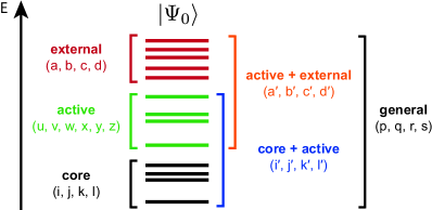
Here, we present a general formulation of the multi-reference ADC theory for the polarization propagator (MR-ADC). We start by dividing the spin-orbitals into three sets: core, active, and external. Figure 1 shows the orbital spaces and the orbital index notation used in this work. We now assume that we have solved the complete active-space self-consistent field (CASSCF) variational problem and computed the reference wavefunction for the ground state. In addition to , our model space contains the excited-state wavefunctions (), which we obtain from the complete active-space configuration interaction computation (CASCI) using the ground-state CASSCF orbitals. We refer to this procedure of constructing the model space as CASCI/CASSCF.
To guide our development of MR-ADC further, we introduce two requirements:
-
•
Requirement 1. At each order of perturbation theory , the -th-order MR-ADC approximation must reduce to the -th-order SR-ADC approximation [ADC(n)] in the limit of the single-determinant and zero active orbitals.
-
•
Requirement 2. The zeroth-order MR-ADC approximation must yield exactly the CASCI/CASSCF excitation energies and transition amplitudes between the ground- () and excited-state (, ) model wavefunctions in the active space.
These two requirements make sure that MR-ADC produces the SR-ADC and the exact (i.e., full configuration interaction) excitation energies and transition amplitudes in the two limits, respectively: (i) zero active orbitals (requirement 1), and (ii) all orbitals are active (requirement 2).
To satisfy the requirement 1, we derive MR-ADC using the effective Liouvillean approach described in Section II that we generalize for multi-determinant reference wavefunctions. Thus, we consider approximations to the ground-state correlated wavefunction in the form:
| (32) | ||||
| (33) |
where the operator generates all internally-contracted excitations between core, active, and external orbitals. Eq. 32 is equivalent to the wavefunction used in internally-contracted multi-reference unitary coupled cluster theory and the related approaches.Kirtman:1981p798 ; Hoffmann:1988p993 ; Yanai:2006p194106 ; Yanai:2007p104107 ; Chen:2012p014108 ; Li:2015p2097 ; Li:2016p164114 As we will discuss in Section V, excitations generated by the operator are linearly-dependent and the redundant amplitudes need to be eliminated.Yanai:2007p104107 ; Evangelista:2011p114102 ; Hanauer:2011p204111 ; Datta:2012p204107 A procedure for removing the redundant amplitudes is described in the Appendix.
To define the MR-ADC perturbative series, we must choose the zeroth-order Hamiltonian . While the choice of is flexible, it must guarantee that the requirement 2 is satisfied. This suggests that must be an interacting Hamiltonian in the active space, rather than a Fock-like one-electron operator. In our MR-ADC development we choose to be the Dyall Hamiltonian,Dyall:1995p4909 ; Angeli:2001p10252 ; Angeli:2001p297 ; Angeli:2004p4043 defined as:
| (34) |
where
| (35) | ||||
| (36) | ||||
| (37) |
The Dyall Hamiltonian includes all active-space terms of the full electronic Hamiltonian (Eq. 16), satisfying the eigenvalue problem
| (38) |
for all CASCI/CASSCF model wavefunctions with eigenvalues , which is a necessary condition for fulfilling the requirement 2. For convenience, we work in the basis of the diagonal core and external generalized Fock operators (, ), where takes the form:
| (39) |
We now consider the expansion of the propagator with respect to the perturbation that defines the MR-ADC approximations. Conveniently, the general form of the MR-ADC equations is equivalent to that of SR-ADC presented in Section II.2. The -th order MR-ADC approximation, which will be termed as MR-ADC(n) henceforth, is defined by truncating the expansion for in Eq. 20 after . The -th-order contribution is given by Eqs. 21, 22, 23, 24 and 25 and the MR-ADC(n) eigenvalue problem can be written as in Eq. 29. Despite general similarities, in MR-ADC, the matrices , , and that compose are evaluated using the multi-reference model wavefunctions , which incorporate the information about the active-space correlation and electronic states into the description of the propagator.
III.2 Perturbative analysis of the MR-ADC equations
In this section, we perform a perturbative analysis of the MR-ADC equations to illustrate the most important features of this theory. To compute the MR-ADC(n) excitation energies and transition amplitudes, we need to evaluate the , , and matrices up to the -th order in perturbation theory. This requires: (i) deriving expressions for the effective Hamiltonian , (ii) constructing the operator manifolds , (iii) solving equations for the -th-order contributions to the amplitudes (Eq. 33), and (iv) evaluating the transformed operators . Since for the polarization propagator and contain the same information, we will only consider and drop the subscript everywhere in the equations.
III.2.1 Zeroth-order contributions
The zeroth-order operators and have a simple form:
| (40) | ||||
| (41) |
where we define . Following procedure outlined in Section II.2, from Eq. 41 we determine that the zeroth-order operators have the form of the single-particle operators . Importantly, must satisfy VAC with respect to the ground-state model wavefunction , i.e. . Since is a CAS-type wavefunction, there is a total of nine different classes of the operators , where indices and belong to different orbitals subspaces (i.e., core, active, or external). Out of nine classes, two classes with only core () or only external () indices are redundant as they do not produce excited configurations when acting on . We do not include these operators in the operator manifold . Among the remaining types, the operators , , and can be added to , while their adjoints contribute to . The last operator class with all active indices () generates excitations in the active space, but does not satisfy VAC with respect to , and thus cannot be included in . These operators require a special treatment in our development.
Expanding the active-space operators in the form , where is a complete set of the active-space eigenoperatorsKutzelnigg:1998p5578 with a property , we express the configurations generated by as:
| (42) |
where the r.h.s. of Eq. 42 is obtained by inserting the resolution of identity over a complete set of the active-space model states in the l.h.s. of that equation. Eq. 42 suggests the form for the coefficients and the eigenoperatorsLowdin:1985p285 :
| (43) |
Since the CASCI/CASSCF model states are orthogonal, the excited-state eigenoperators () automatically fulfill VAC
| (44) |
and thus can be included in the operator manifold . Importantly, choosing in the form of Eq. 43 together with the choice for the zeroth-order Hamiltonian (Eq. 39) ensures that the requirement 2 discussed in Section III.1 is satisfied. The completeness of the operator set is equivalent to the availability of the complete model space . For small active spaces, it is possible to operate with a complete set of such that the set of is complete. However, in most computations, it will be necessary to truncate the set to include only the low-energy states of interest, introducing an approximation (see Section V for details).
We summarize that the operator manifold consists of the four classes of operators:
| (45) |
The zeroth-order MR-ADC matrices have the general form:
| (46) | ||||
| (47) | ||||
| (48) |
Explicit equations for and are shown in the Supporting Information. In contrast to SR-ADC, these matrices are non-diagonal, due to the non-orthogonal nature of the internally-contracted configurations (e.g., ) and the non-diagonal form of the Dyall Hamiltonian. However, the off-diagonal blocks of and corresponding to different types of vanish.
III.2.2 First-order contributions
Expanding the BCH expansions in Eqs. 26 and 27 to the first order, we obtain:
| (49) | ||||
| (50) |
Since is a two-electron operator, the first-order excitation operator only includes up to the two-body terms: . From Eq. 50 we determine the first-order operator manifold , which consists of eight different types of double excitations:
| (51) |
where . The MR-ADC matrices have the following structure:
| (52) | ||||
| (53) | ||||
| (54) |
In the MR-ADC(1) approximation, where , the terms that depend on the double-excitation manifold do not contribute, since the block of the effective Liouvillean matrix is a contribution to . However, these contributions need to be included in MR-ADC(2) and the higher-order approximations. Evaluation of requires the first-order single-excitation (, , ) and (semi-internal) double-excitation (, , ) amplitudes. These amplitudes can be obtained by solving a system of the projected amplitude equations
| (55) | |||
| (56) |
where and . We discuss the solution of these equations in more detail in the Appendix.
III.2.3 Second-order contributions
The second-order operators and have the form:
| (57) | ||||
| (58) |
The second term in Section III.2.3 generates the three-body operators that compose the second-order operator manifold . The MR-ADC matrices contain the following second-order terms:
| (59) | ||||
| (60) | ||||
| (61) |
Terms containing need to be included only in MR-ADC(4) and higher-order approximations. However, all terms involving the double-excitation manifold must be included already in MR-ADC(2). Computation of requires solving for all amplitudes of the and operators, as well as for the single- and semi-internal double-excitation amplitudes of and .
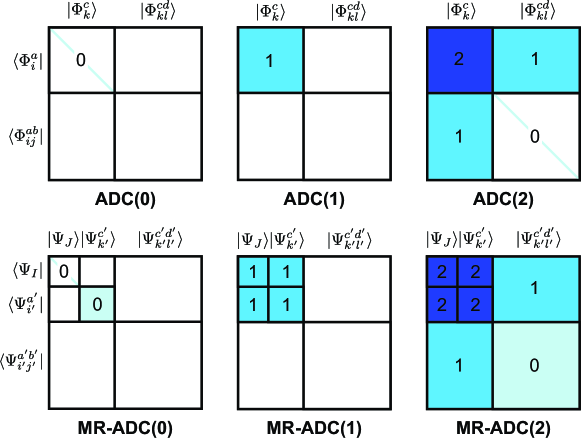
Figure 2 compares the effective Liouvillean matrix for the single-reference ADC(n) and multi-reference MR-ADC(n) approximations (n = 0, 1, 2). Although in MR-ADC there are more excitation classes than in SR-ADC, the perturbative structure of the MR-ADC(n) and ADC(n) matrices is very similar. These matrices become equivalent in the limit of the single-determinant and zero active orbitals.
Finally, we comment about size-extensivity of the MR-ADC(n) approximations. The commutator structure of the MR-ADC equations ensures that all of the terms that appear in these equations are fully linked, which formally guarantees size-consistency of the MR-ADC excitation energies and transition amplitudes at any level of approximation, similar to that of the single-reference ADC. In practice, however, size-consistency can be violated during the numerical solution of the MR-ADC equations as a result of removing redundant excitations of the operator . These size-consistency errors originate from the disconnected terms involving the single and semi-internal amplitudes (e.g., and ) that become non-zero when linear dependencies are eliminated.Hanauer:2011p204111 ; Hanauer:2012p131103 We will investigate the size-consistency errors of the MR-ADC(1) approximation in Section VI.1.
IV Implementation: MR-ADC(1)
We have derived and implemented equations for the MR-ADC(1) approximation as a first step in constructing the hierarchy of the MR-ADC methods. The general structure of the MR-ADC(1) approximation was described in Section III.2 and the explicit equations are shown in the Supporting Information. Although the single-reference ADC(1) energies are equivalent to those obtained from the Tamm-Dancoff approximationFetter2003 (TDA), the MR-ADC(1) and the multi-configurational TDA (MC-TDA)Yeager:1979p77 ; Dalgaard:1980p816 ; Radojevic:1985p2991 ; Sangfelt:1998p4523 ; Nakatani:2014p024108 energies are in general different. This is because in MR-ADC(1) the effective Liouvillean matrix contains additional non-zero terms that depend on the single-excitation (, ) and semi-internal (, , ) amplitudes that are not present in MC-TDA. Neglecting these terms reduces the MR-ADC(1) equations to those of MC-TDA.
The main steps of the MR-ADC(1) implementation for a CASSCF reference wavefunction are summarized below:
-
1.
Choose active space, compute the ground-state CASSCF wavefunction .
-
2.
Using the optimized CASSCF orbitals, compute the energies and the wavefunctions for lowest-energy CASCI states.
-
3.
Compute active-space reduced density matrices (RDMs) for the ground state and transition RDMs between and the excited CASCI states ().
-
4.
Solve linear equations for the single-excitation (, ) and semi-internal (, , ) amplitudes (see the Appendix for details).
-
5.
Compute the overlap () and the effective Liouvillean matrices ().
-
6.
Solve the generalized eigenvalue problem (29) to compute excitation energies.
In the algorithm outlined above, the model space should contain all CASCI states that are important for the problem and spectral region of interest. Evaluation of the matrix elements requires computation of up to the three-particle ground-state RDM (3-RDM) and three-particle transition RDM, which have computational scaling, where is the dimension of the active-space Hilbert space and is the number of active orbitals. In addition, solving the amplitude equations for the semi-internal excitations with three active-space indices ( and ) requires computing the ground-state 4-RDM, which has computational cost. In our implementation, we avoid computation and storage of 4-RDM using the imaginary-time propagation algorithm outlined in the Appendix.
V Computational details
We implemented MR-ADC(1) in a standalone Python program. To obtain one- and two-electron integrals and the CASSCF reference wavefunctions, our program was interfaced with Pyscf.Sun:2018pe1340 The main steps of our implementation are described in Section IV. In all MR-ADC(1) computations, the CASSCF reference molecular orbitals were optimized for the ground electronic state with tight convergence parameters for the energy (10-8 ). These orbitals were used in the following CASCI computation, which produced wavefunctions for the excited states in the active space. We refer to this procedure as CASCI/CASSCF. We denote active spaces used in CASCI/CASSCF as (e, o), where is the number of active electrons and is the number of orbitals. The MR-ADC(1) results were benchmarked against accurate reference data from full configuration interaction (FCI) and density matrix renormalization group (DMRG) and were compared to results from strongly-contracted -electron valence second-order perturbation theory (sc-NEVPT2)Angeli:2001p10252 and its quasidegenerate variant (sc-QD-NEVPT2).Angeli:2004p4043 The NEVPT2 computations were performed using the Orca programNeese:2017pe1327 and employed the state-averaged CASSCF orbitals (SA-CASSCF).
In addition to choosing the active space, the MR-ADC(1) results depend on three parameters: (i) the parameter for the imaginary-time propagation used to compute the semi-internal amplitudes of the effective Hamiltonian, (ii) the thresholds and for removing linear dependencies in the overlap matrices, and (iii) , the number of the CASCI states in the model space.
We refer the interested readers to the Appendix for details about the imaginary-time propagation and the overlap matrices. In short, our imaginary-time algorithm follows the procedure described in Ref. 115. The time propagation is performed using the embedded Runge-Kutta algorithm, which automatically determines the time step based on the accuracy parameter .Press:2007 Since the imaginary-time propagation is a relatively inexpensive step of our algorithm, we use a small value in all computations, which allows to compute numerically accurate semi-internal amplitudes with 10 to 40 imaginary-time steps.
To remove linear dependencies, we first diagonalize the overlap matrices , , and defined in Eqs. 75, 86 and 81, respectively. We then arrange the resulting eigenvalues ( = , , ) in the ascending order and project out the eigenvectors with the smallest that satisfy the following condition:
| (62) |
where the sum in the numerator runs over the truncated and the denominator contains the total sum of . In practice, the diagonalization needs to be performed only for the active-space blocks of , , and with the same core () and external () indices. Our numerical tests indicate that numerical instabilities due to the linear dependencies can be completely eliminated when and are chosen to be 10-8 and 10-3, respectively, which is consistent with the values used in implementations of other internally-contracted multi-reference theories.Yanai:2007p104107 ; Evangelista:2011p114102 ; Hanauer:2011p204111 ; Datta:2012p204107 We use these values in all of our computations. We note that the procedure for removing linear dependencies used in this work treats redundancies in single and double (semi-internal) excitations on equal footing, but is not unique. Other strategies for eliminating linear dependencies can be used, where either one of the excitation classes is omitted or excitations of one class are removed from excitations of another class.Hanauer:2011p204111 We refer to the work by Hanauer and Köhn in Ref. 107 for a detailed numerical analysis of these alternative methods within the framework of internally-contracted multi-reference coupled cluster theory.
| Overlap truncation threshold () | |||||
| State | |||||
| Å | |||||
| S1 | 4.7 | 8.0 | 9.7 | 2.8 | 1.1 |
| S2 | 8.7 | 1.5 | 6.2 | 4.2 | 1.3 |
| S3 | 4.3 | 1.1 | 2.0 | 8.7 | 1.8 |
| S4 | 5.0 | 5.3 | 1.3 | 2.8 | 4.0 |
| Å | |||||
| S1 | 4.0 | 4.1 | 2.1 | 2.2 | 2.2 |
| S2 | 5.3 | 1.5 | 6.9 | 4.2 | 5.8 |
| S3 | 2.2 | 5.5 | 3.2 | 3.3 | 3.2 |
| S4 | 1.0 | 4.0 | 2.9 | 2.9 | 2.8 |
Finally, the MR-ADC(1) results depend on the number of the CASCI states included in the model space (, see Section IV). The optimal value of depends on the system and should include all active-space states in the energy range of interest. In our computations, we usually start with and increase it until the excitation energies for the relevant states are converged. For the systems and active spaces considered in this work, the optimal value of ranged from 20 to 50 states, with the exception of the Be atom with the active space, where we had to use = 80 to obtain converged energies for all excited states. An important feature of MR-ADC(1) is that the excited-state CASCI wavefunctions are only used to compute the transition reduced density matrices and thus can be discarded after their computation is complete.
VI Results
VI.1 Size-consistency of excitation energies
We first examine size-consistency of the MR-ADC(1) energies for a system of two non-interacting water molecules. As we discussed in Section III.2, the MR-ADC approximations are formally size-consistent, but removing redundancies from the cluster operator can give rise to size-consistency errors. Table 1 shows size-consistency errors ( in eV) of the MR-ADC(1) excitation energies for the four lowest-energy singlet excited states of the non-interacting water molecules with two different O–H bond lengths (1.0 and 2.0 Å). Our numerical tests indicate that the size-consistency errors originate from the terms that depend on the core-active and active-external amplitudes (denoted as and in the Appendix) and vanish when these amplitudes are set to zero. To study the effect of the overlap truncation on the magnitude of the size-consistency errors, we computed for different values of the overlap truncation parameter (Section V). For all values of , the errors are small ( eV) with the largest error of only 0.053 eV. Changing from to does not significantly affect the values, most of them change by less than an order of magnitude.
We note that the observed size-consistency errors are intrinsic to the procedure used to project out linear dependencies and are not unique to MR-ADC. For example, Hanauer and KöhnHanauer:2011p204111 demonstrated that eliminating redundancies in the equations of internally-contracted multi-reference coupled cluster theory also gives rise to size-extensivity and size-consistency errors. They developed alternative truncation schemes that allow to reduce or eliminate size-extensivity errors.Hanauer:2012p131103 These schemes can be readily adopted in MR-ADC to remove size-consistency errors, which will be the subject of our future work.
VI.2 Excitation energies of the \ceBe atom
| CASCI/ | CASCI/ | CASCI/ | sc-NEVPT2/ | FCI | |
|---|---|---|---|---|---|
| State | CASSCF | SA(9)-CASSCF | SA(20)-CASSCF | SA(20)-CASSCF | |
| 6.08 | 5.33∗ | 5.38∗ | 5.37∗ | 5.32 | |
| 10.76 | 6.75∗ | 6.69∗ | 6.77∗ | 6.77 | |
| 8.11 | 7.29 | 7.04∗ | 7.14∗ | 7.09 | |
| 17.21 | 8.81 | 7.75 | 7.53 | 7.46 | |
| 18.90 | 12.76 | 11.16 | 9.20 | 8.03 | |
| 2.92 | 2.69∗ | 2.63∗ | 2.73∗ | 2.73 | |
| 11.94 | 6.41∗ | 6.33∗ | 6.46∗ | 6.44 | |
| 7.93 | 7.42 | 7.24∗ | 7.33∗ | 7.30 | |
| 16.73 | 8.38 | 7.39∗ | 7.45∗ | 7.42 | |
| 16.47 | 11.54 | 9.44 | 8.30 | 7.74 | |
| 5.07 | 1.13 | 0.56 | 0.20 | ||
| 4.30 | 1.74 | 1.08 | 0.38 |
| MR-ADC(1) | MR-ADC(1) | MR-ADC(1) | FCI | Experimenta | |
|---|---|---|---|---|---|
| State | () | () | () | ||
| 5.43 | 5.31 | 5.37 | 5.32 | 5.28 | |
| 6.96 | 6.77 | 6.78 | 6.77 | 6.78 | |
| 7.18 | 7.15 | 7.15 | 7.09 | 7.05 | |
| 7.62 | 7.46 | 7.48 | 7.46 | 7.46 | |
| 8.24 | 8.07 | 8.07 | 8.03 | 7.99 | |
| 8.26 | 8.08 | 8.09 | 8.08 | 8.09 | |
| 8.48 | 8.30 | 8.32 | 8.30 | 8.31 | |
| 8.74 | 8.55 | 8.55 | 8.54 | 8.53 | |
| 8.79 | 8.60 | 8.61 | 8.60 | 8.60 | |
| 8.88 | 8.69 | 8.70 | 8.69 | 8.69 | |
| 9.17 | 8.98 | 8.99 | 8.98 | 8.84 | |
| 2.72 | 2.72 | 2.73 | 2.73 | 2.73 | |
| 6.52 | 6.43 | 6.44 | 6.44 | 6.46 | |
| 7.45 | 7.29 | 7.30 | 7.30 | 7.30 | |
| 7.65 | 7.65 | 7.55 | 7.42 | 7.40 | |
| 7.91 | 7.74 | 7.75 | 7.74 | 7.69 | |
| 8.15 | 7.98 | 7.99 | 7.99 | 8.00 | |
| 8.45 | 8.27 | 8.28 | 8.27 | 8.28 | |
| 8.63 | 8.45 | 8.46 | 8.45 | 8.42 | |
| 8.74 | 8.56 | 8.57 | 8.56 | 8.56 | |
| 8.87 | 8.68 | 8.69 | 8.69 | 8.69 | |
| 9.06 | 8.88 | 8.90 | 8.89 | 8.82 | |
| 9.14 | 8.96 | 8.97 | 8.96 | 8.89 | |
| 0.16 | 0.02 | 0.02 | |||
| 0.05 | 0.05 | 0.03 |
-
a
See Ref. 117 for references to experimental results.
In this section, we study the dependence of the MR-ADC(1) results on the size of the active space. In our benchmark, we consider the beryllium atom (Be), for which the accurate results from full configuration interaction (FCI) are available in the literature.Graham:1998p6544 We use the same basis set as in Ref. 117 and employ three active spaces in our reference CASSCF computations, including all orbitals in parenthesis: , ), and . The largest active space corresponds to (2e, 13o).
We first investigate accuracy of the Be excitation energies computed using conventional methods, such as CASCI and strongly-contracted NEVPT2 (sc-NEVPT2). Table 2 shows results of CASCI and sc-NEVPT2 obtained using the largest active space. The CASCI energies were computed using the ground-state CASSCF orbitals (CASCI/CASSCF), as well as the CASSCF orbitals averaged over lowest-energy states [CASCI/SA()-CASSCF, = 9 and 20]. For sc-NEVPT2, only the SA()-CASSCF orbitals were used. For all electronic states, the CASCI excitation energies strongly depend on the choice of molecular orbitals. In particular, using the ground-state CASSCF orbitals leads to very large mean absolute errors () and standard deviations () of 5.07 and 4.30 eV, respectively, relative to FCI. These errors are substantially reduced when using the state-averaged CASSCF orbitals. In this case, the best agreement with the FCI benchmark results is observed for states that were included in state-averaging (errors of 0.11 eV), while much larger errors (up to 3 eV) are obtained for the remaining states. Incorporating the description of dynamic correlation using the sc-NEVPT2/SA()-CASSCF method further reduces the errors, yielding excitation energies in excellent agreement with FCI for states included in state-averaging. Although sc-NEVPT2 improves the description of the remaining states, their computed transition energies are significantly overestimated (up to 1.17 eV).
We now turn our attention to the MR-ADC(1) results presented in Table 3. Importantly, while CASCI and sc-NEVPT2 can only be used to compute energies of transitions between orbitals in the active space, MR-ADC(1) provides information about excitations between all orbitals. Although MR-ADC(1) is the simplest approximation in the MR-ADC hierarchy, its accuracy can be improved by increasing the size of the active space. Table 3 demonstrates that the MR-ADC(1) excitation energies converge towards the FCI limit as the active space is expanded from to . Including more orbitals in the active space also improves the description of excitations between active and external orbitals. For example, the error in excitation energy for the state reduces from 0.17 eV to 0.01 eV by increasing the active space from to . Overall, for the largest active space, the MR-ADC(1) results are in a close agreement with FCI, with mean absolute errors () and standard deviations () of 0.02 and 0.03 eV, respectively. Although the MR-ADC(1) method used the ground-state CASSCF orbitals, its and computed using the smallest () active space (0.16 and 0.05 eV, respectively) are already smaller than those of sc-NEVPT2/SA()-CASSCF employing the largest active space (0.20 and 0.38 eV).
Interestingly, the MR-ADC(1) excitation energies agree very closely to the energies from multi-configurational linear response theory (MC-LR) reported in Ref. 117 for almost all states but the state, where the difference of 0.05 eV is observed. Although both theories are based on the first-order approximation to the polarization propagator, MC-LR is formulated as a non-Hermitian eigenvalue problem, whereas the MR-ADC(1) energies are computed by diagonalizing a Hermitian matrix of a smaller dimension.
VI.3 Avoided crossing in \ceLiF
Next, we test MR-ADC(1) for the description of an avoided crossing between the ground and the excited states of LiF.Finley:1998p299 ; Nakano:2002p1166 ; Angeli:2004p4043 ; Granovsky:2011p214113 At short bond distances, the wavefunctions of these two states are dominated by the ionic and covalent configurations, respectively. As the bond distance increases, the potential energy curves of the two states closely approach each other and their wavefunctions strongly interact, exchanging their character. In this section, we use the 6-31+G* basis setHariharan:1973p213 ; Clark:1983p294 and compare the MR-ADC(1) results to those obtained from FCI, state-averaged CASSCF (SA-CASSCF), strongly-contracted quasidegenerate NEVPT2 (sc-QD-NEVPT2), and multi-configurational Tamm-Dancoff approximation (MC-TDA). As described in Section IV, MC-TDA can be considered as an approximation to MR-ADC(1) where all terms that depend on the single- and semi-internal double-excitation amplitudes are neglected. The FCI results were computed using the semistochastic heat-bath configuration interaction algorithm (SHCI) implemented in the Dice program.Holmes:2016p3674 ; Sharma:2017p1595 ; Holmes:2017p164111 The orbital of fluorine was not correlated in the SHCI computations. All active-space methods used the (6e, 6o) active space. In SA-CASSCF and sc-QD-NEVPT2, both and states were included in state-averaging to compute the reference CASSCF orbitals. In MR-ADC(1) and MC-TDA, the CASSCF orbitals were optimized for the ground state.
| State | TDA | CASCI/CASSCF | MR-ADC(1) | sc-NEVPT2 | DMRGa |
|---|---|---|---|---|---|
| 1.30 | 2.31 | 1.97 | 1.42 | 1.29 | |
| b | 4.08 | 4.08 | 2.45 | 2.17 | |
| b | 4.07 | 4.04 | 2.73 | 2.45 | |
| 6.42 | 6.27 | 5.98 | 4.83 | 4.61 | |
| 2.41 | 0.97 | 0.64 | 0.34 | 0.21 | |
| b | 3.17 | 3.17 | 1.56 | 1.29 | |
| 1.08 | 1.39 | 1.28 | 1.35 | 1.29 | |
| b | 3.74 | 3.57 | 2.85 | 2.65 | |
| 7.35 | 8.03 | 7.17 | 7.02 | 6.66 | |
| 2.01 | 1.27 | 1.03 | 0.21 | ||
| 2.11 | 0.59 | 0.69 | 0.10 |
-
a
The DMRG results employing the (12e, 28o) active space are from Ref. 125.
-
b
Excited state with double excitation character, absent in TDA.
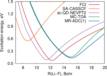
Figure 3 plots the excitation energy () for various bond distances computed using MR-ADC(1), MC-TDA, sc-QD-NEVPT2, SA-CASSCF, and FCI. The FCI curve exhibits a minimum corresponding to an avoided crossing at 12.25 with = 0.07 eV. SA-CASSCF shows the worst agreement with FCI predicting an avoided crossing at 8.75 with = 0.55 eV. MR-ADC(1) qualitatively reproduces the shape of the FCI curve locating an avoided crossing at 15.25 with = 0.12 eV. Although at each geometry the MR-ADC(1) error in is large (0.3 to 0.5 eV), relative to FCI, the MR-ADC(1) curve is quite parallel to FCI for the short ( 10 ) and long ( 16 ) bond distances. In addition, MR-ADC(1) demonstrates a significant improvement over the reference CASCI/CASSCF results, which do not exhibit an avoided crossing at any geometry. The MC-TDA curve is quite close to MR-ADC(1) for the short bond distances ( 14 ), but significantly deviates from MR-ADC(1) at the longer distances ( 16 ), showing larger non-parallelity errors relative to FCI. The best results are shown by the sc-QD-NEVPT2 method, which locates an avoided crossing at 11.5 with = 0.09 eV, indicating the importance of the two-electron dynamic correlation effects that are not included in MR-ADC(1).
VI.4 Doubly excited states in \ceC2
Finally, we consider a challenging example of the \ceC2 molecule, whose excited states require very accurate description of static and dynamic correlation.Roos:1987p399 ; Bauschlicher:1987p1919 ; Watts:199p6073 ; Abrams:2004p9211 ; Wouters:2014p1501 ; Holmes:2017p164111 Table 4 reports the MR-ADC(1) vertical excitation energies for \ceC2 at near equilibrium bond distance ( = 2.4 ) computed using the cc-pVDZ basis set.Dunning:1989p1007 In addition, we report results from the single-reference Tamm-Dancoff approximation (TDA), CASCI computed using the ground-state CASSCF orbitals (CASCI/CASSCF), and strongly-contracted NEVPT2 (sc-NEVPT2). For all active-space methods, the CASSCF reference wavefunction was computed using the (8e, 8o) active space. As a benchmark, we employ the accurate density matrix renormalization group (DMRG) results obtained by Wouters et al.Wouters:2014p1501
All low-lying electronic states of \ceC2 considered in Table 4 have a significant multi-reference character. This is evidenced by the TDA method, which incorrectly predicts the ground state and completely misses four out of nine excited states, due to their doubly excited nature. On the contrary, the MR-ADC(1) method correctly assigns the ground state to be and provides excitation energies for the doubly excited states. However, for most of the electronic states, the MR-ADC(1) energies significantly overestimate the DMRG results and are close to CASCI/CASSCF. Although for some states (e.g., or ) the MR-ADC(1) and CASCI/CASSCF results are virtually identical, for other states MR-ADC(1) predicts somewhat lower excitation energies, reducing the error relative to DMRG by up to 0.35 eV, with an exception of the state where a substantial improvement of 0.86 eV is observed. The large errors of MR-ADC(1) are due to the missing description of the two-electron dynamic correlation between core, active, and external orbitals, which is very important in the excited states of \ceC2. This is evidenced by the results of the sc-NEVPT2 method, which are in a much closer agreement with DMRG ( = 0.21, = 0.10 eV) than MR-ADC(1) ( = 1.03, = 0.69 eV). The two-electron dynamic correlation effects will be incorporated in the second-order MR-ADC approximation (MR-ADC(2)) and are expected to significantly lower the excitation energies, reducing the errors relative to reference values.
VII Conclusions
In this work, we considered a multi-reference formulation of the algebraic diagrammatic construction theory (MR-ADC) for excited states of strongly correlated systems. The MR-ADC approach is an alternative to multi-reference perturbation theories and multi-reference propagator methods and has several attractive properties: (i) it allows for including and systematically improving the description of the dynamic correlation effects outside of the active space, (ii) it describes electronic transitions involving all orbitals (i.e., core, active, and external), (iii) it is based on the Hermitian eigenvalue problem and thus ensures that the excitation energies have real values, (iv) it enables efficient computation of spectroscopic properties (such as transition amplitudes and spectral densities), and (v) allows for simulations of various spectroscopic processes (e.g., valence or core excitations, photoionization). In contrast to the original (single-reference) ADC theory, MR-ADC is more reliable in situations where the multi-reference effects are important in the ground or excited electronic states. Our formulation of MR-ADC is based one the effective Liouvillean formalism of Mukherjee and Kutzelnigg, originally developed for the single-determinant reference wavefunctions.Mukherjee:1989p257 By generalizing this formalism to multi-determinant states, we arrived at the MR-ADC formulation, which naturally reduces to the conventional ADC theory in the single-reference limit. We performed a perturbative analysis of MR-ADC and outlined a procedure for constructing MR-ADC approximations at each order in perturbation theory.
As a first step in defining the hierarchy of the MR-ADC methods, we presented an implementation of the first-order MR-ADC approximation for the polarization propagator (MR-ADC(1)) and benchmarked its results for two non-interacting water molecules, excitation energies of the Be atom, an avoided crossing in \ceLiF, and doubly excited states in \ceC2. For the water molecules, we showed that the MR-ADC(1) excitation energies exhibit small size-consistency errors, which originate due to removing linear dependencies in the overlap metric. For the Be atom, we demonstrated that the MR-ADC(1) results converge to the full configuration interaction limit with increasing active space size. In a study of \ceLiF, we showed that MR-ADC(1) qualitatively correctly describes an avoided crossing due to the mixing of the ionic and covalent configurations. For \ceC2, MR-ADC(1) predicts excitation energies of the doubly excited states, but shows large errors relative to reference values, missing the description of the two-electron dynamic correlation outside of the active space. These correlation effects are incorporated in the second-order MR-ADC approximation and are expected to significantly improve the results.
We envision many possible extensions of the current work. An immediate extension is the development of the second-order MR-ADC(2) approximation for the polarization propagator, which will incorporate the description of the two-electron dynamic correlation effects that are essential for accurate predictions of the excitation energies and excited-state properties. A further direction is to develop the MR-ADC methods for simulations of other spectroscopic properties, such as photoelectron, X-ray absorption or two-photon absorption spectra. Although the conventional ADC theory has been applied to these problems,Schirmer:1983p1237 ; Barth:1985p867 ; Knippenberg:2012p064107 MR-ADC is expected to be more reliable for systems with challenging electronic structure, such as open-shell molecules and transition metal complexes. Additionally, for systems containing heavy elements, it will be important to combine MR-ADC with the description of relativistic effects. Finally, MR-ADC can be combined with density matrix renormalization group or selected configuration interaction approaches,Huron:1973p5745 ; Chan:2011p465 which will enable simulations of spectroscopic properties of multi-reference systems with a large number of strongly correlated electrons. Work along these directions is ongoing in our group.
VIII Acknowledgements
This work was supported by the start-up funds provided by the Ohio State University. The author would like to thank Francesco Evangelista for comments on this manuscript and insightful discussions.
IX Appendix: MR-ADC(1) amplitude equations
Here, we describe how to solve the MR-ADC(1) amplitude equations. The general form of the equations is shown in Eqs. 55 and 56. The action of the first-order effective Hamiltonian on the reference state can be written as:
| (63) |
where and is the ground-state CASCI/CASSCF energy.
IX.1 Core-external amplitudes
First, we consider equations for the core-external and amplitudes. For brevity, we omit the perturbation order in our notation, e.g. . Projecting Eq. 63 by and on the left, the amplitude equations can be written in a tensor form:
| (64) |
where is a standard notation for the core-external single excitations used in -electron valence perturbation theory (NEVPT)Angeli:2001p10252 ; Angeli:2001p297 ; Angeli:2004p4043 and the tensors are defined as:
| (65) |
| (66) |
| (67) |
The elements of reduce to
| (68) | ||||
| (69) | ||||
| (70) | ||||
| (71) |
For the elements of , we obtain:
| (72) | ||||
| (73) |
To solve Eq. 64, we first consider the generalized eigenvalue problem for the matrix :
| (74) |
where the overlap metric has a general form
| (75) |
Defining , the matrix in Eq. 74 can be expressed as:
| (76) |
This allows us to obtain expression for the amplitudes in terms of the eigenvalues , eigenvectors and the overlap matrices:
| (77) |
Solving the eigenvalue problem (74) requires diagonalizing the overlap metric and projecting out the eigenvectors corresponding to small eigenvalues (see Section V for details). Since the matrix elements in Eqs. 68, 69, 70 and IX.1 are zero for or , Eq. 74 can be solved for each block with and independently, which greatly reduces the cost of computing the amplitudes. Although in this work we only deal with the first-order amplitudes, we note that in MR-ADC the extraction of linearly independent amplitudes has to be done separately at each order of perturbation theory.
IX.2 Avoiding computation of 4-RDM for the core-active and active-external amplitudes
Next, we consider the core-active amplitudes and belonging to the excitation class of NEVPT. The amplitude equations can be obtained by projecting Eq. 63 by the and configurations and can be written in the form similar to Eq. 64: . As previously, this system of linear equations can be solved by diagonalizing and inverting the matrix . However, evaluation of requires the four-particle reduced density matrix (4-RDM), which has a steep computational scaling with the number of active orbitals and the dimension of the active-space Hilbert space .
Here, we present a different algorithm, which does not require computation of 4-RDM. We start by multiplying both sides of Eq. 63 by and and set the corresponding projections to zero. For example, for the projection we obtain:
| (78) |
where we expressed the operator resolvent using a Laplace transform as an integral over imaginary time .Sokolov:2016p064102 The resulting amplitude equations can be written in the matrix form:
| (79) |
where the tensor product is carried out over the unique sets of amplitudes only (i.e., , ) and the tensors are defined as:
| (80) |
| (81) |
| (82) |
The matrix elements of can be evaluated by the imaginary-time propagation of the active-space state , where
| (83) |
and integrating Eq. 82 numerically over a set of time steps . The details of the imaginary-time propagation algorithm can be found in Section V and in Ref. 115. Once is determined, we diagonalize the overlap metric , project out the linearly dependent eigenvectors with small eigenvalues, and compute the amplitudes according to Eq. 79.
For the active-external excitations and corresponding to the excitation class of NEVPT, the amplitude equations have a similar form:
| (84) |
| (85) |
| (86) |
| (87) |
| (88) |
Avoiding the evaluation of 4-RDM lowers the computational cost of solving the core-active and active-external amplitude equations from to and , respectively, where is the number of time steps in imaginary time ( 10 to 40), is the number of core orbitals, and is the number of external orbitals.
References
- (1) A. Szabo and N. Ostlund, Modern Quantum Chemistry: Introduction to Advanced Electronic Structure Theory (Macmillan, New York, 1982).
- (2) T. Helgaker, P. Jørgensen, and J. Olsen, Molecular Electronic Structure Theory (John Wiley & Sons, Ltd., New York, 2000).
- (3) A. L. Fetter and J. D. Walecka, Quantum theory of many-particle systems (Dover Publications, 2003).
- (4) W. H. Dickhoff and D. Van Neck, Many-body theory exposed!: propagator description of quantum mechanics in many-body systems (World Scientific Publishing Co., 2005).
- (5) H. Nakatsuji and K. Hirao, J. Chem. Phys. 68, 2053 (1978).
- (6) H. Nakatsuji, Chem. Phys. Lett. 67, 329 (1979).
- (7) M. Nooijen and R. J. Bartlett, J. Chem. Phys. 106, 6441 (1997).
- (8) M. Nooijen and R. J. Bartlett, J. Chem. Phys. 107, 6812 (1997).
- (9) C. D. Sherrill and H. F. Schaefer, Adv. Quant. Chem. 34, 143 (1999).
- (10) J. Geertsen, M. Rittby, and R. J. Bartlett, Chem. Phys. Lett. 164, 57 (1989).
- (11) D. C. Comeau and R. J. Bartlett, Chem. Phys. Lett. 207, 414 (1993).
- (12) J. F. Stanton and R. J. Bartlett, J. Chem. Phys. 98, 7029 (1993).
- (13) A. I. Krylov, Annu. Rev. Phys. Chem. 59, 433 (2008).
- (14) O. Goscinski and B. Weiner, Phys. Scr. 21, 385 (1980).
- (15) B. Weiner and O. Goscinski, Int. J. Quantum Chem. 18, 1109 (1980).
- (16) M. D. Prasad, S. Pal, and D. Mukherjee, Phys. Rev. A 31, 1287 (1985).
- (17) B. Datta, D. Mukhopadhyay, and D. Mukherjee, Phys. Rev. A 47, 3632 (1993).
- (18) P. O. Löwdin, Int. J. Quantum Chem. 5, 231 (1970).
- (19) E. S. Nielsen, P. Jørgensen, and J. Oddershede, J. Chem. Phys. 73, 6238 (1980).
- (20) E. Sangfelt, H. A. Kurtz, N. Elander, and O. Goscinski, J. Chem. Phys. 81, 3976 (1984).
- (21) K. L. Bak, H. Koch, J. Oddershede, O. Christiansen, and S. P. A. Sauer, J. Chem. Phys. 112, 4173 (2000).
- (22) D. Mukherjee and W. Kutzelnigg, in Many-Body Methods in Quantum Chemistry (Springer, Berlin, Heidelberg, Berlin, Heidelberg, 1989), pp. 257–274.
- (23) M. Nooijen and J. G. Snijders, Int. J. Quantum Chem. 44, 55 (1992).
- (24) M. Nooijen and J. G. Snijders, Int. J. Quantum Chem. 48, 15 (1993).
- (25) M. Nooijen and J. G. Snijders, J. Chem. Phys. 102, 1681 (1995).
- (26) R. Moszynski, P. S. Żuchowski, and B. Jeziorski, Collect. Czech. Chem. Commun. 70, 1109 (2005).
- (27) T. Korona, Phys. Chem. Chem. Phys. 12, 14977 (2010).
- (28) K. Kowalski, K. Bhaskaran-Nair, and W. A. Shelton, J. Chem. Phys. 141, 094102 (2014).
- (29) J. Schirmer, Phys. Rev. A 26, 2395 (1982).
- (30) J. Schirmer, L. S. Cederbaum, and O. Walter, Phys. Rev. A 28, 1237 (1983).
- (31) J. Schirmer, Phys. Rev. A 43, 4647 (1991).
- (32) F. Mertins and J. Schirmer, Phys. Rev. A 53, 2140 (1996).
- (33) J. Schirmer and A. B. Trofimov, J. Chem. Phys. 120, 11449 (2004).
- (34) A. Dreuw and M. Wormit, WIREs Comput. Mol. Sci. 5, 82 (2014).
- (35) J. Liu, A. Asthana, L. Cheng, and D. Mukherjee, J. Chem. Phys. 148, 244110 (2018).
- (36) A. Tarantelli and L. S. Cederbaum, in Many-Body Methods in Quantum Chemistry (Springer, Berlin, Heidelberg, Berlin, Heidelberg, 1989), pp. 233–256.
- (37) J. D. McClain, J. Lischner, T. J. Watson, Jr., D. A. Matthews, E. Ronca, S. G. Louie, T. C. Berkelbach, and G. K.-L. Chan, Phys. Rev. B 93, 235139 (2016).
- (38) K. Bhaskaran-Nair, K. Kowalski, and W. A. Shelton, J. Chem. Phys. 144, 144101 (2016).
- (39) M. F. Lange and T. C. Berkelbach, J. Chem. Theory Comput. 14, 4224 (2018).
- (40) T. C. Berkelbach, J. Chem. Phys. 149, 041103 (2018).
- (41) H. Sekino and R. J. Bartlett, Int. J. Quantum Chem. 26, 255 (1984).
- (42) H. Koch, H. J. A. Jensen, P. Jørgensen, and T. Helgaker, J. Chem. Phys. 93, 3345 (1990).
- (43) H. Koch and P. Jørgensen, J. Chem. Phys. 93, 3333 (1990).
- (44) H.-J. Werner and W. Meyer, J. Chem. Phys. 73, 2342 (1980).
- (45) H.-J. Werner, J. Chem. Phys. 74, 5794 (1981).
- (46) P. J. Knowles and H.-J. Werner, Chem. Phys. Lett. 115, 259 (1985).
- (47) K. Wolinski, H. L. Sellers, and P. Pulay, Chem. Phys. Lett. 140, 225 (1987).
- (48) K. Hirao, Chem. Phys. Lett. 190, 374 (1992).
- (49) H.-J. Werner, Mol. Phys. 89, 645 (1996).
- (50) J. P. Finley, P. Å. Malmqvist, B. O. Roos, and L. Serrano-Andrés, Chem. Phys. Lett. 288, 299 (1998).
- (51) K. Andersson, P. Å. Malmqvist, B. O. Roos, A. J. Sadlej, and K. Wolinski, J. Phys. Chem. 94, 5483 (1990).
- (52) K. Andersson, P. Å. Malmqvist, and B. O. Roos, J. Chem. Phys. 96, 1218 (1992).
- (53) C. Angeli, R. Cimiraglia, S. Evangelisti, T. Leininger, and J.-P. P. Malrieu, J. Chem. Phys. 114, 10252 (2001).
- (54) C. Angeli, R. Cimiraglia, and J.-P. P. Malrieu, Chem. Phys. Lett. 350, 297 (2001).
- (55) C. Angeli, S. Borini, M. Cestari, and R. Cimiraglia, J. Chem. Phys. 121, 4043 (2004).
- (56) A. Banerjee, J. W. Kenney, and J. Simons, Int. J. Quantum Chem. 16, 1209 (1979).
- (57) D. L. Yeager and P. Jørgensen, Chem. Phys. Lett. 65, 77 (1979).
- (58) E. Dalgaard, J. Chem. Phys. 72, 816 (1980).
- (59) D. L. Yeager, J. Olsen, and P. Jørgensen, Faraday Symp. Chem. Soc. 19, 85 (1984).
- (60) R. L. Graham and D. L. Yeager, J. Chem. Phys. 94, 2884 (1991).
- (61) D. L. Yeager, in Applied Many-Body Methods in Spectroscopy and Electronic Structure (Springer, Boston, MA, Boston, MA, 1992), pp. 133–161.
- (62) J. A. Nichols, D. L. Yeager, and P. Jørgensen, J. Chem. Phys. 80, 293 (1998).
- (63) V. F. Khrustov and D. E. Kostychev, Int. J. Quantum Chem. 88, 507 (2002).
- (64) S. Chattopadhyay, U. S. Mahapatra, and D. Mukherjee, J. Chem. Phys. 112, 7939 (2000).
- (65) S. Chattopadhyay and D. Mukhopadhyay, J. Phys. B: At. Mol. Opt. Phys. 40, 1787 (2007).
- (66) T.-C. Jagau and J. Gauss, J. Chem. Phys. 137, 044116 (2012).
- (67) P. K. Samanta, D. Mukherjee, M. Hanauer, and A. Köhn, J. Chem. Phys. 140, 134108 (2014).
- (68) D. Datta and M. Nooijen, J. Chem. Phys. 137, 204107 (2012).
- (69) M. Nooijen, O. Demel, D. Datta, L. Kong, K. R. Shamasundar, V. Lotrich, L. M. Huntington, and F. Neese, J. Chem. Phys. 140, 081102 (2014).
- (70) L. M. J. Huntington and M. Nooijen, J. Chem. Phys. 142, 194111 (2015).
- (71) Y. A. Aoto and A. Köhn, J. Chem. Phys. 144, 074103 (2016).
- (72) Y. Kurashige and T. Yanai, J. Chem. Phys. 135, 094104 (2011).
- (73) Y. Kurashige, J. Chalupský, T. N. Lan, and T. Yanai, J. Chem. Phys. 141, 174111 (2014).
- (74) S. Guo, M. A. Watson, W. Hu, Q. Sun, and G. K.-L. Chan, J. Chem. Theory Comput. 12, 1583 (2016).
- (75) S. Sharma, G. Knizia, S. Guo, and A. Alavi, J. Chem. Theory Comput. 13, 488 (2017).
- (76) T. Yanai, M. Saitow, X.-G. Xiong, J. Chalupský, Y. Kurashige, S. Guo, and S. Sharma, J. Chem. Theory Comput. 13, 4829 (2017).
- (77) L. Freitag, S. Knecht, C. Angeli, and M. Reiher, J. Chem. Theory Comput. 13, 451 (2017).
- (78) A. Y. Sokolov, S. Guo, E. Ronca, and G. K.-L. Chan, J. Chem. Phys. 146, 244102 (2017).
- (79) M. K. MacLeod and T. Shiozaki, J. Chem. Phys. 142, 051103 (2015).
- (80) W. Kutzelnigg and D. Mukherjee, J. Chem. Phys. 90, 5578 (1989).
- (81) W. Kutzelnigg, J. Chem. Phys. 77, 3081 (1982).
- (82) R. J. Bartlett, S. A. Kucharski, and J. Noga, Chem. Phys. Lett. 155, 133 (1989).
- (83) J. D. Watts, G. W. Trucks, and R. J. Bartlett, Chem. Phys. Lett. 157, 359 (1989).
- (84) D. Kats, D. Usvyat, and M. Schütz, Phys. Rev. A 83, 062503 (2011).
- (85) G. Wälz, D. Kats, D. Usvyat, T. Korona, and M. Schütz, Phys. Rev. A 86, 052519 (2012).
- (86) D. Lefrancois, M. Wormit, and A. Dreuw, J. Chem. Phys. 143, 124107 (2015).
- (87) D. Lefrancois, D. Tuna, T. J. Martínez, and A. Dreuw, J. Chem. Theory Comput. 13, 4436 (2017).
- (88) P. O. Löwdin, Adv. Quant. Chem. 17, 285 (1985).
- (89) P. O. Löwdin, Int. J. Quantum Chem. 2, 867 (1968).
- (90) P. O. Löwdin, Phys. Rev. 139, A357 (1965).
- (91) O. Goscinski and B. Lukman, Chem. Phys. Lett. 7, 573 (1970).
- (92) R. Manne, Chem. Phys. Lett. 45, 470 (1977).
- (93) E. Dalgaard, Int. J. Quantum Chem. 15, 169 (1979).
- (94) J. Schirmer, A. B. Trofimov, and G. Stelter, J. Chem. Phys. 109, 4734 (1998).
- (95) A. B. Trofimov and J. Schirmer, J. Chem. Phys. 123, 144115 (2005).
- (96) J. H. Starcke, M. Wormit, and A. Dreuw, J. Chem. Phys. 130, 024104 (2009).
- (97) S. Knippenberg, D. R. Rehn, M. Wormit, J. H. Starcke, I. L. Rusakova, A. B. Trofimov, and A. Dreuw, J. Chem. Phys. 136, 064107 (2012).
- (98) M. Pernpointner, J. Chem. Phys. 140, 084108 (2014).
- (99) B. Kirtman, J. Chem. Phys. 75, 798 (1998).
- (100) M. R. R. Hoffmann and J. Simons, J. Chem. Phys. 88, 993 (1988).
- (101) T. Yanai and G. K.-L. Chan, J. Chem. Phys. 124, 194106 (2006).
- (102) T. Yanai and G. K.-L. Chan, J. Chem. Phys. 127, 104107 (2007).
- (103) Z. Chen and M. R. R. Hoffmann, J. Chem. Phys. 137, 014108 (2012).
- (104) C. Li and F. A. Evangelista, J. Chem. Theory Comput. 11, 2097 (2015).
- (105) C. Li and F. A. Evangelista, J. Chem. Phys. 144, 164114 (2016).
- (106) F. A. Evangelista and J. Gauss, J. Chem. Phys. 134, 114102 (2011).
- (107) M. Hanauer and A. Köhn, J. Chem. Phys. 134, 204111 (2011).
- (108) K. G. Dyall, J. Chem. Phys. 102, 4909 (1995).
- (109) M. Hanauer and A. Köhn, J. Chem. Phys. 137, 131103 (2012).
- (110) V. Radojević and W. R. Johnson, Phys. Rev. A 31, 2991 (1985).
- (111) E. Sangfelt, R. R. Chowdhury, B. Weiner, and Y. Öhrn, J. Chem. Phys. 86, 4523 (1998).
- (112) N. Nakatani, S. Wouters, D. Van Neck, and G. K.-L. Chan, J. Chem. Phys. 140, 024108 (2014).
- (113) Q. Sun, T. C. Berkelbach, N. S. Blunt, G. H. Booth, S. Guo, Z. Li, J. Liu, J. D. McClain, E. R. Sayfutyarova, S. Sharma, S. Wouters, and G. K.-L. Chan, WIREs Comput. Mol. Sci. 8, e1340 (2018).
- (114) F. Neese, WIREs Comput. Mol. Sci. 8, e1327 (2017).
- (115) A. Y. Sokolov and G. K.-L. Chan, J. Chem. Phys. 144, 064102 (2016).
- (116) W. H. Press, S. A. Teukolsky, W. T. Vetterling, and B. P. Flannery, Numerical Recipes: The Art of Scientific Computing (Cambridge University Press, New York, 1986).
- (117) R. L. Graham, D. L. Yeager, J. Olsen, P. Jørgensen, R. Harrison, S. Zarrabian, and R. J. Bartlett, J. Chem. Phys. 85, 6544 (1998).
- (118) H. Nakano, R. Uchiyama, and K. Hirao, J. Comput. Chem. 23, 1166 (2002).
- (119) A. A. Granovsky, J. Chem. Phys. 134, 214113 (2011).
- (120) P. C. Hariharan and J. A. Pople, Theoret. Chim. Acta 28, 213 (1973).
- (121) T. Clark, J. Chandrasekhar, G. W. Spitznagel, and P. v. R. Schleyer, J. Comput. Chem. 4, 294 (1983).
- (122) A. A. Holmes, N. M. Tubman, and C. J. Umrigar, J. Chem. Theory Comput. 12, 3674 (2016).
- (123) S. Sharma, A. A. Holmes, G. Jeanmairet, A. Alavi, and C. J. Umrigar, J. Chem. Theory Comput. 13, 1595 (2017).
- (124) A. A. Holmes, C. J. Umrigar, and S. Sharma, J. Chem. Phys. 147, 164111 (2017).
- (125) S. Wouters, W. Poelmans, P. W. Ayers, and D. Van Neck, Comput. Phys. Commun. 185, 1501 (2014).
- (126) B. O. Roos, Adv. Chem. Phys. 69, 399 (1987).
- (127) C. W. Bauschlicher Jr and S. R. Langhoff, J. Chem. Phys. 87, 2919 (1987).
- (128) J. D. Watts and R. J. Bartlett, J. Chem. Phys. 96, 6073 (1992).
- (129) M. L. Abrams and C. D. Sherrill, J. Chem. Phys. 121, 9211 (2004).
- (130) T. H. Dunning Jr, J. Chem. Phys. 90, 1007 (1989).
- (131) A. Barth and J. Schirmer, J. Phys. B: At. Mol. Phys. 18, 867 (1985).
- (132) B. Huron, J.-P. P. Malrieu, and P. Rancurel, J. Chem. Phys. 58, 5745 (1973).
- (133) G. K.-L. Chan and S. Sharma, Annu. Rev. Phys. Chem. 62, 465 (2011).