Growth on Two Limiting Essential Resources in a Self-Cycling Fermentor

Abstract.

A system of impulsive differential equations with state-dependent impulses is used to model the growth of a single population on two limiting essential resources in a self-cycling fermentor. Potential applications include water purification and biological waste remediation. The self-cycling fermentation process is a semi-batch process and the model is an example of a hybrid system. In this case, a well-stirred tank is partially drained, and subsequently refilled using fresh medium when the concentration of both resources (assumed to be pollutants) falls below some acceptable threshold. We consider the process successful if the threshold for emptying/refilling the reactor can be reached indefinitely without the time between successive emptying/refillings becoming unbounded and without interference by the operator. We prove that whenever the process is successful, the model predicts that the concentrations of the population and the resources converge to a positive periodic solution. We derive conditions for the successful operation of the process that are shown to be initial condition dependent and prove that if these conditions are not satisfied, then the reactor fails. We show numerically that there is an optimal fraction of the medium drained from the tank at each impulse that maximizes the output of the process.

Ting-Hao Hsu^∗, Tyler Meadows^∗, Lin Wang^†, and Gail S. K. Wolkowicz^∗‡

Department of Mathematics and Statistics^∗

McMaster University

1280 Main Street West

Hamilton, Ontario

Canada, L8S 4K1

Department of Mathematics and Statistics^†

University of New Brunswick

Tilley Hall, 9 MacAulay Lane

PO Box 4400

Fredericton, New Brunswick

Canada, E3B 5A3

1. Introduction

The self-cycling fermentation (SCF) process can be described in two stages: In the first stage, a well-stirred tank is filled with resources and inoculated with microorganisms that consume the resources. When a threshold concentration of one or more indicator quantities is reached, the second stage is initiated. The first stage is a batch culture [5]. During the second stage, the tank is partially drained, and subsequently refilled with fresh resources before repeating the first stage.

SCF is most often applied to wastewater treatment processes, where the goal is to reduce the concentration of one or more harmful compounds [10, 16]. In this application the concentration of harmful compounds is the most reasonable threshold quantity, since acceptable concentrations would typically be given by some government agency. More recently, the SCF process has been used as a means to improve production of some biologically derived compounds [20, 23]. In these instances, dissolved $\mathrm{O_{2}}$ content, or dissolved $\mathrm{CO_{2}}$ content have been used as threshold quantities, since they are good indicators of when the microorganism approaches the stationary phase in its growth cycle. In both scenarios, the end goal is to maximize the amount of substrate processed by the reactor, while maintaining stable operating conditions. SCF has also been used to culture synchronized microbial cultures [17], where stability of the operating conditions is much more important than output of the reactor. It is the first scenario that we model, i.e. we consider the case that the microbial population is used to reduce two harmful compounds to an acceptable level.

Assuming that the time taken to empty and refill the tank is negligible, we can model the SCF process using a system of impulsive differential equations. Smith and Wolkowicz [18] used this approach to model the growth of a single species with one limiting resource. Fan and Wolkowicz [7] extended this model to include the possibility that the resource is limiting at large concentrations. Córdova-Lepe, Del Valle, and Robledo [6] also modeled single species growth in the SCF process, but used impulse dependent impulse times instead of the state dependent impulses used by the other models. For references on the theory of impulsive differential equations, see e.g. [1, 2, 3, 9, 15].

When there are two (or more) resources in limited supply, it is important to think about how the resources interact to promote growth. If any of the resources can be used interchangeably with the same outcome, we say the resources are substitutable. For instance, both glucose and fructose are carbon sources for many bacteria, and can fulfill the same purpose in bacterial growth. If all of the resources are required in some way for growth, and the bacteria will die out if any were missing, we say the resources are essential. For instance, both carbon and nitrogen are required for growth of many bacteria, but glucose cannot be used as a nitrogen source, so some other compound such as nitrate is required. Growth and competition with two essential resources has been studied in the chemostat [4], in the chemostat with delay [12], and in the unstirred chemostat [24]. In all of the aforementioned studies, the interaction of essential resources is through Liebig’s law of the minimum [22]. To illustrate the law of the minimum, consider a barrel with several staves of unequal length. Growth is limited by the resource in shortest supply in the same way that the capacity of the barrel is limited by length of the shortest stave.

In this paper we investigate the dynamics of the self-cycling fermentation process in a semi-batch culture with two essential resources that are assumed to be pollutants. The goal is to reduce both pollutant concentrations to acceptable levels. In section 2 we introduce the model. In section 3 we analyze the system of ordinary differential equations (ODEs) associated with the model introduced in section 2. In section 4 we analyze the system of impulsive differential equations introduced in section 2, and obtain our main results: Theorem 4.6, which gives necessary and sufficient conditions for the existence of a unique periodic orbit, and Theorem 4.14, which summarizes all of the possible long term dynamics of the model. In section 5 we demonstrate numerically that the emptying/refilling fraction can be used to maximize the output of the SCF process. In section 6 we summarize our results and discuss the implications of our analysis. All figures were produced using Matlab [13].

2. Model Formulation

For a given function $y(t)$ and time $\tau$, using the standard notation for impulsive equations we denote by $\Delta y(\tau)=y(\tau^{+})-y(\tau^{-})$, where

$$y(\tau^{+})\equiv\lim_{t\rightarrow\tau^{+}}y(t)\ \ \ \mbox{and}\ \ \ y(\tau^{-})\equiv\lim_{t\rightarrow\tau^{-}}y(t).$$

Our model takes the form

$$\left.\begin{array}[]{ccl}\frac{ds_{1}(t)}{dt}&=&-\frac{1}{Y_{1}}\min\{f_{1}(s_{1}(t)),f_{2}(s_{2}(t))\}x(t),\\ \frac{ds_{2}(t)}{dt}&=&-\frac{1}{Y_{2}}\min\{f_{1}(s_{1}(t)),f_{2}(s_{2}(t))\}x(t),\\ \frac{dx(t)}{dt}&=&(-D+\min\{f_{1}(s_{1}(t)),f_{2}(s_{2}(t))\})x(t),\end{array}\right\}\quad t\neq t_{k}$$

                                                                    (1)

$$\left.\begin{array}[]{ccl}\Delta s_{1}(t_{k})&=&-rs_{1}(t_{k}^{-})+rs_{1}^{\mathrm{in}},\\ \Delta s_{2}(t_{k})&=&-rs_{2}(t_{k}^{-})+rs_{2}^{\mathrm{in}},\\ \Delta x(t_{k})&=&-rx(t_{k}^{-}),\end{array}\right\}\quad t=t_{k}$$

where $t_{k}$ are the times at which

$$\text{either}\quad\big{(}s_{1}(t_{k})=\bar{s}_{1},s_{2}(t_{k})\leq\bar{s}_{2}\big{)}\quad\text{or}\quad\big{(}s_{1}(t_{k})\leq\bar{s}_{1},s_{2}(t_{k})=\bar{s}_{2}\big{)}.$$ (2)

Here, $t$ denotes time. The variables $s_{i},\ i=1,2$ denote the concentration of the limiting resources (assumed to be pollutants) in the fermentor as a function of $t$, with associated parameters $Y_{i}$, the cell yield constants, $s^{\mathrm{in}}_{i}$, the concentrations of each limiting resource in the medium added to the tank at the beginning of each new cycle, and $\bar{s}_{i}$ the threshold concentrations of limiting resource that trigger the emptying and refilling process. Since we are considering the scenario where both $s_{1}$ and $s_{2}$ are pollutants, the emptying and refilling process is only triggered when both concentrations reach the acceptable levels $\bar{s}_{1}$ and $\bar{s}_{2}$ set by some environmental protection agency. The variable $x$ denotes the biomass concentration of the population of microorganisms that consume the resource at time $t$, assumed to have death rate $D$. The emptying/refilling fraction is denoted by $r$. It is assumed that $D>0,\ 0<r<1$  and for $i=1,2,\ Y_{i}>0,$ and $s^{\mathrm{in}}_{i}>\bar{s}_{i}>0$.

We call the times $t_{k}>0$, impulse times, and when they exist they form an increasing sequence that we denote $\{t_{k}\}_{k=1}^{N}$. If (2) is satisfied at $t=0$ or $s_{i}(0)<\bar{s}_{i},\ i=1,2$, then we assume that there is an immediate impulse at time $t=0$. We consider the process to be successful if $N=\infty$ and the time between impulses, $t_{k}-t_{k-1}$ remains bounded. We consider the process a failure if either there are a finite number of impulses, and hence $N$ is finite, or if the time between impulses becomes unbounded.

The two resources are assumed to be limiting essential resources (see e.g., Tilman [21] or Grover [8]) also called complementary resources (see Leon and Tumpson [11]), and as in those studies we use Liebig’s law of the minimum [22] to model the uptake and growth of the microbial population.

We assume that each response function $f_{j}(s)$, $j=1,2$, in (1) satisfies:

1. $f_{j}:\mathbb{R}_{+}\to\mathbb{R}_{+}$ is continuously differentiable;

2. $f_{j}(0)=0$ and $f_{j}^{\prime}(s)>0$ for $s>0$;

Define $\lambda_{i}$, $i=1,2$, to be the value of each resource that satisfies $f_{i}(\lambda_{i})=D$, and refer to each $\lambda_{i}$ as a “break-even concentration”. If $f_{j}$ is bounded below $D$, then we define the corresponding $\lambda_{j}=\infty$.

Between two consecutive impulses the system is governed by a system of ordinary differential equations (ODE) that models a batch fermentor [5],

$$\frac{ds_{1}(t)}{dt} = -\frac{1}{Y_{1}}\min\{f_{1}(s_{1}(t)),f_{2}(s_{2}(t))\}x(t),$$

$$\frac{ds_{2}(t)}{dt} = -\frac{1}{Y_{2}}\min\{f_{1}(s_{1}(t)),f_{2}(s_{2}(t))\}x(t),$$ (3)

$$\frac{dx(t)}{dt} = (-D+\min\{f_{1}(s_{1}(t)),f_{2}(s_{2}(t))\})x(t).$$

We will refer to system (3) as the associated ODE system.

3. Dynamics of System (3)

First we show that system (3) is well-posed.

Proposition 3.1.

Given any positive initial conditions $(s_{1}(0),s_{2}(0),x(0))$, the solution $(s_{1}(t),s_{2}(t),x(t))$ of (3) is defined for all $t\geq 0$ and remains positive.

Furthermore, $\lim_{t\to\infty}(s_{1}(t),s_{2}(t),x(t))$ exists, is initial condition dependent,
$\lim_{t\to\infty}x(t)=0$, and $\lim_{t\to\infty}s_{i}(t)<\lambda_{i}$ for at least one $i\in\{1,2\}$.

Proof.

Since the vector field in (3) is locally Lipschitz, the positivity of $(s_{1}(t),s_{2}(t),x(t))$ follows from the standard theory for the existence and uniqueness of solutions of ODEs (see e.g.,  [14]). Also observe that

$$\frac{d}{dt}\left(x(t)+\frac{Y_{1}}{2}s_{1}(t)+\frac{Y_{2}}{2}s_{2}(t)\right)=-Dx(t)<0,$$

so the solution $(s_{1}(t),s_{2}(t),x(t))$ exists and is bounded for $t$ in $[0,\infty)$.

From (3), $s_{i}^{\prime}(t)<0$, $i=1,2$. By the positivity of $s_{i}(t)$, $\lim_{t\to\infty}s_{i}(t)\geq 0$ exists. Denote $\lim_{t\to\infty}s_{i}(t)=s_{i}^{*}$, $i=1,2$.

We claim that $\min\{f_{1}(s_{1}^{*}),f_{2}(s_{2}^{*})\}<D$. Suppose not. Then, $\min\{f_{1}(s_{1}^{*}),f_{2}(s_{2}^{*})\}\geq D$. Since both $s_{1}(t)$ and $s_{2}(t)$ are strictly decreasing functions, it follows that $\min\{f_{1}(s_{1}(t)),f_{2}(s_{2}(t))\}>D$ for all $t\geq 0$. From the equation of $x^{\prime}(t)$ in (3), $x(t)$ would be a strictly increasing function. Then, $s_{1}^{\prime}(t)<\frac{-D}{Y_{1}}x(0)$ for all $t\geq 0$, contradicting the positivity of $s_{1}(t)$. Hence, $s_{i}^{*}<\lambda_{i}$ for at least one $i\in\{1,2\}$.

Since $\min\{f_{1}(s_{1}^{*}),f_{2}(s_{2}^{*})\}<D$, define $\gamma=-D+\min\{f_{1}(s_{1}^{*}),f_{2}(s_{2}^{*})\}<0$. By the equation for $x^{\prime}(t)$ in (3), $x^{\prime}(t)<\frac{\gamma}{2}x(t)<0$, for all sufficiently large $t$. Hence $x(t)\to 0$ as $t\to\infty$. ∎

Note that from (3), $Y_{1}\frac{ds_{1}}{dt}=Y_{2}\frac{ds_{2}}{dt}$. Define

$$R_{12}=\frac{Y_{2}}{Y_{1}}\quad\text{and}\quad R_{21}=\frac{Y_{1}}{Y_{2}}=\frac{1}{R_{12}}.$$ (4)

Then, every trajectory of (3) satisfies $\frac{ds_{2}}{ds_{1}}=R_{21}$.

Lemma 3.2.

Let $(s_{1}(t),s_{2}(t),x(t))$ be a solution of (3) on an interval $t\in[t_{0},t_{1}]$ with positive initial conditions. Then,

$$s_{1}(t)=s_{1}({t_{0}})+R_{12}(s_{2}(t)-s_{2}({t_{0}})),$$ (5)

or equivalently

$$s_{2}(t)=s_{2}({t_{0}})+R_{21}(s_{1}(t)-s_{1}({t_{0}})),$$ (6)

$$x(t_{1})-x(t_{0})=Y_{1}\int_{s_{1}(t_{1})}^{s_{1}(t_{0})}\left(1-\frac{D}{\min\big{\{}f_{1}(v),f_{2}\big{(}s_{2}(t_{1})+R_{21}(v-s_{1}(t_{1}))\big{)}\big{\}}}\right)dv,$$ (7)

or equivalently

$$x(t_{1})-x(t_{0})=Y_{2}\int_{s_{2}(t_{1})}^{s_{2}(t_{0})}\left(1-\frac{D}{\min\{f_{1}\big{(}s_{1}(t_{1})+R_{12}(v-s_{2})\big{)},f_{2}(v)\}}\right)dv.$$ (8)

Proof.

Solving the separable ODE, $\frac{ds_{1}}{ds_{2}}=R_{12}$, yields (5), and solving $\frac{ds_{2}}{ds_{1}}=R_{21}$, yields (6). Dividing the $s_{1}^{\prime}(t)$ equation in (3) by the $x^{\prime}(t)$ equation, substituting for $s_{2}(t)$ using (6), and then integrating both sides, yields (7). We obtain (8) similarly. ∎

4. Analysis of the Full System (1)

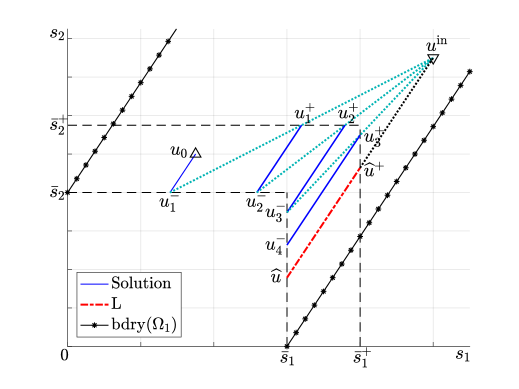
Figure 1. $u_{0}=(s_{1}^{0},s_{2}^{0})$, indicated by $\triangle$, is the initial condition. $u^{\mathrm{in}}=(s_{1}^{\mathrm{in}},s_{2}^{\mathrm{in}})$, indicated by $\bigtriangledown$, is the input concentration. $u_{k}^{\pm}=(s_{1}(t_{k}^{\pm}),s_{2}(t_{k}^{\pm})),\ k=1,2,\dots,$ satisfy $u_{k}^{+}=(1-r)u_{k}^{-}+ru^{\mathrm{in}}$, where $u^{\mathrm{in}}=(s_{1}^{\mathrm{in}},s_{2}^{\mathrm{in}})$. Each connected piece of the solution has slope $R_{21}$. $\widehat{u}=(\bar{s}_{1},\widehat{s_{2}})=(\bar{s}_{1},s_{2}^{\mathrm{in}}-R_{21}(s_{1}^{\mathrm{in}}-\bar{s}_{1})$ and $\widehat{u}^{+}=(\bar{s}_{1}^{+},\widehat{s}_{2}^{+})=((1-r)\bar{s}_{1}+rs^{\mathrm{in}}_{1},s_{2}^{\mathrm{in}}-(1-r)R_{21}(s^{\mathrm{in}}_{1}-\bar{s}_{1}))$. The set $\Omega_{1}$ lies above and to the right of $\Gamma^{-}$ and between the two lines with slope $R_{21}$, through $(0,\bar{s}_{2})$ and $(\bar{s}_{1},0)$, respectively.

First we visualize solutions of (1) in the $s_{1}$-$s_{2}$ plane as illustrated in Figure 1. Given any solution $(s_{1}(t),s_{2}(t),x(t))$ of (1) with positive initial conditions, let $t_{0}=0$ and let $t_{k}$, $k\in\mathbb{N}$, denote the $k$th impulse time if it exists.

Let $u_{k}^{\pm}=(s_{1}(t_{k}^{\pm}),s_{2}(t_{k}^{\pm}))$. By (6), the trajectory of $(s_{1}(t),s_{2}(t))$, $t\in(t_{k},t_{k+1})$, is a line segment with slope $R_{21}$ and endpoints $u_{k}^{+}$ and $u_{k+1}^{-}$. The conditions for impulses to occur are given in (2). Therefore, each point $u_{k}^{-}$ lies in the following union of the two horizontal and vertical line segments:

$$\Gamma^{-}\equiv\big{\{}(s_{1},\bar{s}_{2}):s_{1}\in[0,\bar{s}_{1}]\big{\}}\cup\big{\{}(\bar{s}_{1},s_{2}):s_{2}\in[0,\bar{s}_{2}]\big{\}}.$$

Define

$$u^{\mathrm{in}}=(s_{1}^{\mathrm{in}},s_{2}^{\mathrm{in}})\quad\mbox{and}\quad\bar{s}_{i}^{+}=(1-r)\bar{s}_{i}+rs_{i}^{\mathrm{in}},\ i=1,2.$$

By the definition of $\Delta s_{i}$ given in (1),

$$u_{k}^{+}=(1-r)u_{k}^{-}+ru^{\mathrm{in}}.$$ (9)

This implies that each $u_{k}^{+}$ lies in the following union of horizontal and vertical line segments:

$$\Gamma^{+}\equiv\big{\{}(s_{1},\bar{s}_{2}^{+}):s_{1}\in[0,\bar{s}_{1}^{+}]\big{\}}\cup\big{\{}(\bar{s}_{1}^{+},s_{2}):s_{2}\in[0,\bar{s}_{2}^{+}]\big{\}}.$$

Therefore, if impulses occur indefinitely, then the total trajectory of $(s_{1}(t),s_{2}(t))$, $t\in[t_{1},\infty)$, is a countable union of line segments with slope $R_{21}$ and endpoints in $\Gamma^{-}\cup\Gamma^{+}$, (i.e., $u_{k}^{+}\in\Gamma^{+}$ and $u_{k}^{-}\in\Gamma^{-}$.)

For any positive solution $(s_{1}(t),s_{2}(t),x(t))$ of (1) with $(s_{1}(0),s_{2}(0))$ lying between the coordinate axes and $\Gamma^{-}$, i.e., $0\leq s_{1}(0)\leq\bar{s}_{1}$ and $0\leq s_{2}(0)\leq\bar{s}_{2}$, an impulse occurs immediately at $t=0$, and so, after at most a finite number of impulses, $(s_{1}(0^{+}),s_{2}(0^{+}))$ lies above or to the right of $\Gamma^{-}$. In the rest of this section, we therefore assume $(s_{1}(0),s_{2}(0))$ lies above or to the right of $\Gamma^{-}$, i.e., $s_{i}(0)>\bar{s}_{i},$ for at least one $i\in\{1,2\}$.

The following proposition asserts that system (1) does not exhibit the phenomenon of beating. That is, the system possesses no solution with impulse times that form an increasing sequence with a finite accumulation point.

Proposition 4.1.

Assume that $(s_{1}(t),s_{2}(t),x(t))$ is a positive solution of (1) with an infinite number of impulse times, $\{t_{k}\}_{k=1}^{\infty}$. Then $\lim_{k\to\infty}t_{k}=\infty$.

Proof.

Between impulses, $s_{1}$ and $s_{2}$ are strictly decreasing for all $x(t)>0$, and therefore we can solve the first equation in (3) for the time between impulses:

$$t_{k+1}-t_{k}=Y_{1}\int_{s_{1}(t_{k+1})}^{s_{1}(t_{k})}\frac{1}{\min\big{\{}f_{1}(v),f_{2}(s_{2}(t_{k+1})+R_{21}(v-s_{1}(t_{k+1}))\big{\}}\;X_{k}(v)}dv$$ (10)

where $X_{k}(v)$ is defined by $X_{k}(s_{1}(t))=x(t)$ for $t\in(t_{k},t_{k+1})$.

To show that $\{t_{k}\}_{k=1}^{\infty}$ has no finite accumulation point, it suffices to show that there exists positive constants, $M_{1}$, $M_{2}$ and $m$, such that

$$s_{1}(t_{k}^{+})-s_{1}(t_{k+1}^{-})>m\quad\text{for}\ k=1,2,\dots$$

and

$$\min\{f_{1}(s_{1}(t)),f_{2}(s_{2}(t))\}<M_{1},\quad x(t)<M_{2},\quad\text{for}\ t\geq 0,$$

since then the difference $t_{k+1}-t_{k}$ is greater than $\frac{Y_{1}m}{M_{1}M_{2}}$.

Since $s_{1}(t_{k}^{-})\leq\bar{s}_{1}$, $s_{2}(t_{k}^{-})\leq\bar{s}_{2}$, and either $s_{1}(t_{k}^{+})=\bar{s}_{1}^{+}$ or $s_{2}(t_{k}^{+})=\bar{s}_{2}^{+}$, we have

$$\text{either}\quad s_{1}(t_{k}^{+})-s_{1}(t_{k+1}^{-})\geq\bar{s}_{1}^{+}-\bar{s}_{1}\quad\text{or}\quad s_{2}(t_{k}^{+})-s_{2}(t_{k+1}^{-})\geq\bar{s}_{2}^{+}-\bar{s}_{2}.$$

From (5) it follows that

$$s_{1}(t_{k}^{+})-s_{1}(t_{k+1}^{-})\geq\min\{\bar{s}_{1}^{+}-\bar{s}_{1},R_{12}(\bar{s}_{2}^{+}-\bar{s}_{2})\}\equiv m.$$

Since after the first impulse occurs, $(s_{1}(t),s_{2}(t))$ is bounded by $\Gamma^{+}$, the existence of $M_{1}$ follows from the continuity of $f_{1}$ and $f_{2}$. By (7), there exists $M_{0}>0$ such that

$$x(t)<x(t_{k}^{+})+M_{0},\quad\text{for}\ t\in(t_{k},t_{k+1}).$$ (11)

From the relation that $x(t_{k}^{+})=rx(t_{k}^{-})$, we obtain

$$x(t_{k+1}^{+})<r(x(t_{k}^{+})+M_{0}),\quad\text{for}\ k=1,2,\dots$$

By the comparison principle applied to $x(t_{k})$ and the sequence $\{y_{k}\}$ defined by $y_{0}=x(0)$ and $y_{k+1}=r(y_{k}+M_{0})$, $k=1,2,\dots$,

$$\limsup_{k\to\infty}x(t_{k}^{+})\leq\lim_{k\to\infty}y_{k}=\frac{rM_{0}}{1-r}.$$ (12)

The existence of $M_{2}$ follows from (11) and (12). ∎

Define $\Omega_{1}$ to be the set of points $(s_{1}^{0},s_{2}^{0})$ such that, for some $x^{0}>0$, the forward trajectory of the solution of (3) with initial value $(s_{1}^{0},s_{2}^{0},x^{0})$ intersects $\Gamma^{-}$. Then the boundary of $\Omega_{1}$ is the union of $\Gamma^{-}$ and the two lines of slope $R_{21}$ passing through $(\bar{s}_{1},0)$ and $(0,\bar{s}_{2})$, respectively. Then,

$$\Omega_{1}=\left\{(s_{1},s_{2}):\begin{aligned} &s_{1}>\bar{s}_{1}\;\text{or}\;s_{2}>\bar{s}_{2},\;\text{and}\\ &s_{2}-\bar{s}_{2}<R_{21}s_{1},\;s_{2}>R_{21}(s_{1}-\bar{s}_{1})\end{aligned}\right\}.$$

Define $\Omega_{0}$ to be the open set complementary to $\Omega_{1}$ in the first quadrant above and to the right of $\Gamma^{-}$. Then,

$$\Omega_{0}=\left\{(s_{1},s_{2}):\begin{aligned} &s_{1}>\bar{s}_{1}\;\text{or}\;s_{2}>\bar{s}_{2},\;\text{and}\\ &s_{2}-\bar{s}_{2}>R_{21}s_{1}\;\text{or}\;s_{2}<R_{21}(s_{1}-\bar{s}_{1})\end{aligned}\right\}.$$

Remark 4.2.

The sets $\Omega_{0}$ and $\Omega_{1}$ do not include the marginal cases where $(s_{1}(0),s_{2}(0))$ lies on the lines of slope $R_{21}$ passing through $(\bar{s}_{1},0)$ or $(0,\bar{s}_{1})$. If $(s_{1}(0),s_{2}(0))$ lies on one of these lines and $s_{i}(0)>0$ for $i=1,2$, then no impulses occur, since the solution curve does not reach $\Gamma^{-}$ in finite time. If $(s_{1}(0),s_{2}(0))=(\bar{s}_{1},0)$ or $(s_{1}(0),s_{2}(0))=(0,\bar{s}_{2})$, then an impulse occurs immediately, and $(s_{1}(0^{+}),s_{2}(0^{+}))$ may be in either $\Omega_{0}$ or $\Omega_{1}$, depending on the location of $u^{\mathrm{in}}$.

In the following case, the fermentation process fails.

Lemma 4.3.

If $(s_{1}(t),s_{2}(t),x(t))$ is a solution of (1) with $(s_{1}(0),s_{2}(0))\in\Omega_{0}$, then no impulses occur.

Proof.

Since $\Omega_{0}$ is complementary to $\Omega_{1}$, $(s_{1}(t),s_{2}(t))\notin\Gamma^{-}$ for any $t\geq 0$, and hence no impulses occur. ∎

Next we define a Lyapunov-type function

$$V(s_{1},s_{2})=Y_{2}(s_{2}^{\mathrm{in}}-s_{2})-Y_{1}(s_{1}^{\mathrm{in}}-s_{1}).$$ (13)

Then,

$$\Omega_{1}=\left\{(s_{1},s_{2}):\begin{aligned} &s_{1}>\bar{s}_{1}\;\text{or}\;s_{2}>\bar{s}_{2},\;\text{and}\\ &V(0,\bar{s}_{2})<V(s_{1},s_{2})<V(\bar{s}_{1},0)\end{aligned}\right\}$$

and

$$\Omega_{0}=\left\{(s_{1},s_{2}):\begin{aligned} &s_{1}>\bar{s}_{1}\;\text{or}\;s_{2}>\bar{s}_{2},\;\text{and}\\ &V(s_{1},s_{2})<V(0,\bar{s}_{2})\;\text{or}\;V(s_{1},s_{2})>V(\bar{s}_{1},0)\end{aligned}\right\}.$$

Note that the level sets of $V$ are straight lines with slope $R_{21}$ in the $s_{1}$-$s_{2}$ plane. For any fixed value of $s_{1}$, $V(s_{1},s_{2})$ is a decreasing function of $s_{2}$, and for any fixed value of $s_{2}$, $V(s_{1},s_{2})$ is an increasing function of $s_{1}$.

Lemma 4.4.

Assume $(s_{1}(t),s_{2}(t),x(t))$ is a solution of (1) with positive initial conditions. Let $t_{0}=0$ and $t_{k}$, $k\in\mathbb{N}$, denote the $k$th impulse time, if it exists; otherwise set $t_{k}=\infty$. Define $V(t)=V(s_{1}(t),s_{2}(t))$. Then,

1. $\frac{d}{dt}V(t)=0$ for $t\in(t_{k},t_{k+1})$,

2. $V(t_{k}^{+})=(1-r)V(t_{k}^{-})$, if $t_{k}<\infty$.

Proof.

(i) By the equations for $ds_{i}/dt$ in (3),

$$\frac{d}{dt}V(t)=\left(\frac{Y_{2}}{Y_{2}}-\frac{Y_{1}}{Y_{1}}\right)\min\{f_{1}(s_{1}(t)),f_{2}(s_{2}(t))\}x(t)=0.$$

(ii) Substituting (9) into (13),

$$V(t_{k}^{+})=(1-r)(s_{1}(t_{k}^{-})-s_{1}^{\mathrm{in}},s_{2}(t_{k}^{-})-s_{2}^{\mathrm{in}})\cdot(Y_{1},-Y_{2})=(1-r)V(t_{k}^{-}),$$

where $\cdot$ denotes the inner product in $\mathbb{R}^{2}$. ∎

By the definition of $V(s_{1},s_{2})$ in (13) and Lemma 4.4, the line

$$\{(s_{1},s_{2}):V(s_{1},s_{2})=0\}=\{(s_{1}^{\mathrm{in}}+vY_{2},s_{2}^{\mathrm{in}}+vY_{1}):v\in\mathbb{R}\}$$ (14)

is invariant under (3) for all $x(0)$. By symmetry, we may assume the point $(\bar{s}_{1},\bar{s}_{2})$ lies on or above this invariant line, i.e., $V(\bar{s}_{1},\bar{s}_{2})\leq 0$, or

$$s_{2}^{\mathrm{in}}-\bar{s}_{2}\leq R_{21}(s_{1}^{\mathrm{in}}-\bar{s}_{1}).$$ (15)

Next we show that in the case that $(s_{1}^{\mathrm{in}},s_{2}^{\mathrm{in}})$ lies in $\Omega_{0}$, once again the fermentation process is doomed to fail.

Lemma 4.5.

If $(s_{1}^{\mathrm{in}},s_{2}^{\mathrm{in}})\in\Omega_{0}$, then every solution of (1) with positive initial conditions has at most finitely many impulses.

Proof.

Note that, $V(s_{1}^{\mathrm{in}},s_{2}^{\mathrm{in}})=0$, so the condition $(s_{1}^{\mathrm{in}},s_{2}^{\mathrm{in}})\notin\Omega_{1}$ implies that either $V(0,\bar{s}_{2})>0$ or $V(\bar{s}_{1},0)<0$. Since $V(0,\bar{s}_{2})<V(\bar{s}_{1},\bar{s}_{2})\leq 0$, by assumption (15), $V(\bar{s}_{1},0)<0$.

We proceed using proof by contradiction. Suppose that a solution $(s_{1}(t),s_{2}(t),x(t))$ of (1) with positive initial conditions has infinitely many impulses. Denote the impulse times by $t_{1}<t_{2}<\cdots$. By Lemma 4.4(ii), $V(s_{1}(t_{k}^{-}),s_{2}(t_{k}^{-}))\to 0$ as $k\to\infty$. Hence, $V(s_{1}(t_{k}^{-}),s_{2}(t_{k}^{-}))>V(\bar{s}_{1},0)$ for some $k\geq 1$. By Lemma 4.3, no more impulses can occur. ∎

In the case of $(s_{1}^{\mathrm{in}},s_{2}^{\mathrm{in}})\in\Omega_{1}$, under assumption (15), the line given by (14) intersects $\Gamma^{-}$ at the point $(\bar{s}_{1},\widehat{s}_{2})$ given by

$$\widehat{s}_{2}=s_{2}^{\mathrm{in}}-R_{21}(s_{1}^{\mathrm{in}}-\bar{s}_{1}).$$

Define $L$ to be the portion of the line given by (14) from the point $(\bar{s}_{1},\widehat{s}_{2})$ to its image via the impulsive map, namely

$$L =\{(s_{1},s_{2}):\bar{s}_{1}\leq s_{1}\leq\bar{s}_{1}^{+},\;V(s_{1},s_{2})=0\}$$

$$=\{(s_{1},s_{2}):\bar{s}_{1}\leq s_{1}\leq\bar{s}_{1}^{+},\;s_{2}=\widehat{s}_{2}+R_{21}(s_{1}-\bar{s}_{1})\}.$$

Then $L$ is invariant under (1) for all $x(0)$.

4.1. Existence of Periodic Orbits

Next we investigate under what conditions the reactor has a periodic solution and the process has the potential to succeed.

We regard the emptying/refilling fraction $r\in(0,1)$ as a variable. Without loss of generality, from now on we assume that $(\bar{s}_{1},\bar{s}_{2})$ lies on or above $L$. Otherwise, from (15), by symmetry we can relabel the resources. Therefore, the right endpoint of $L$ is $(\bar{s}_{1}^{+}(r),\widehat{s}_{2}^{+}(r))$ given by

$$\bar{s}_{1}^{+}(r)=(1-r)\bar{s}_{1}+rs_{1}^{\mathrm{in}}\quad\text{and}\quad\widehat{s}_{2}^{+}(r)=(1-r)\widehat{s}_{2}+rs_{2}^{\mathrm{in}}.$$

By (7), the net change in $x(t)$ over one cycle with impulse at $(\bar{s}_{1},\widehat{s}_{2})$ is

$$\mu(r)=Y_{1}\int_{\bar{s}_{1}}^{\bar{s}_{1}^{+}(r)}\left(1-\frac{D}{\min\{f_{1}(v),f_{2}(\widehat{s}_{2}+R_{21}(v-\bar{s}_{1}))\}}\right)dv.$$ (16)

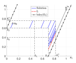
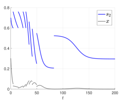
Figure 2. No periodic solution exists, and the $x$-component of every solution tends to $0$ as $t\to\infty$. In the simulation, the response functions are $f_{i}(s_{i})=\frac{m_{i}s_{i}}{a_{i}+s_{i}}$, $i=1,2$, with $(m_{1},m_{2},a_{1},a_{2})=(2,2,1.4,1.2)$. The parameters are $(Y_{1},Y_{2},D)=(2,0.7,0.5)$ and $(\bar{s}_{1},\bar{s}_{2},s_{1}^{\mathrm{in}},s_{2}^{\mathrm{in}},r)=(0.7,0.6,1,1,0.4)$. The initial condition is $u_{0}=(s_{1}(0),s_{2}(0),x(0))=(0.1,0.7,0.3)$. After a finite number of impulses, the orbit converges before reaching the threshold for an impulse, indicated by $\square$. The value of $\mu(r)\approx-0.08<0$.

We prove the following theorem concerning the existence and the uniqueness of periodic solutions.

Theorem 4.6.

Assume $(s_{1}^{\mathrm{in}},s_{2}^{\mathrm{in}})\in\Omega_{1}$. If $r\in(0,1)$ and $\mu(r)>0$, then system (1) has a periodic orbit that is unique up to time translation and has one impulse per period. On a periodic orbit, $x(t_{k}^{+})=\frac{(1-r)}{r}\mu(r)$ and $x(t_{k}^{-})=\frac{1}{r}\mu(r)$, for all  $k\in\mathbb{N}$.

If $\mu(r)\leq 0$, then system (1) has no periodic orbits.

See Figure 2 for an illustration of the case with $\mu(r)<0$.

Proof.

Suppose there is a positive periodic solution $(s_{1}(t),s_{2}(t),x(t))$. Since (3) has no periodic orbits, the solution has at least one impulse. By periodicity there are infinitely many impulses. Denote the impulse times by $t_{1}<t_{2}<\cdots$ and the number of impulses within a period by $N$. Then $x(t_{N+k}^{\pm})=x(t_{k}^{\pm})$ for all $k\in\mathbb{N}$. By (1),

$$x(t_{k+1}^{-})=x(t_{k}^{+})+\mu(r)\quad\text{and}\quad x(t_{k}^{+})=(1-r)x(t_{k}^{-}).$$

Thus,

$$x(t_{k+1}^{-})=(1-r)x(t_{k}^{-})+\mu(r).$$ (17)

If $x(t_{1}^{-})>\mu(r)$ (resp. $x(t_{1}^{+})<\mu(r)$), then from (17) it can be shown by induction that $x(t_{k}^{-})$ is a strictly decreasing (resp. strictly increasing) sequence, contradicting $x(t_{N+k}^{-})=x(t_{k}^{-})$. Hence, on any periodic orbit there is only one impulse, and it follows from (17), on a periodic orbit $x(t_{k}^{-})=\frac{1}{r}\mu(r)$ for all $k\in\mathbb{N}$. Therefore, $\mu(r)>0$, since the solution must be positive, and if a periodic orbit exists it is unique.

If $\mu(r)>0$, the solution of (1) with initial condition $(\bar{s}_{1}^{+},\widehat{s}_{2}^{+},\frac{1-r}{r}\mu(r))$ is periodic, since if$x(t_{k+1}^{-})=\frac{1}{r}\mu(r)$, then $x(t_{k+1}^{+})=\frac{1-r}{r}\mu(r)$ and if $x(t_{k}^{+})=\frac{1-r}{r}\mu(r)$, then $x(t_{k+1}^{-})=\frac{1}{r}\mu(r)$. ∎

Proposition 4.7.

If $\mu(1)>0$, then there exists a unique $r^{*}\in[0,1)$ such that $\mu(r)>0$ for all $r\in(r^{*},1]$ and $\mu(r)\leq 0$ for all $r\in(0,r^{*}].$

Proof.

Let

$$r_{*}=\max\{r\in[0,1]:\mu(v)\leq 0\;\;\forall\;v\in[0,r]\}.$$ (18)

Note that $r_{*}$ is well-defined, since $\mu(r)$ is continuous and $\mu(0)=0$. By definition, $\mu(r)\leq 0$ for all $r\in[0,r_{*}]$. Since $\mu(r)$ is continuous, if $\mu(1)>0$ then $r_{*}<1$. Furthermore, $\mu(r)>0$ for all $r\in(r_{*},1]$, since $f_{1}(s_{1})$ and $f_{2}(s_{2})$ are monotone increasing, and so the integrand in (16) with $v=\bar{s}_{1}^{+}(r_{*})$ must be positive. Otherwise, $r_{*}$ can be increased, contradicting definition (18). By the monotonicity of $f_{1}(s_{1})$ and $f_{2}(s_{2})$, the integrand in (16) with $v=\bar{s}_{1}^{+}(r)$ remains positive for $r_{*}<r\leq 1$. Hence, $\mu(r)>0$ for $r\in(r_{*},1]$. ∎

Remark 4.8.

If $\lambda_{1}\leq\bar{s}_{1}$ and $\lambda_{2}\leq\widehat{s}_{2}$, then $\mu(r)>0$ for all $r\in(0,1)$, i.e., $r_{*}=0$, because the integrand in (16) is then positive for all $v\in(\bar{s}_{1},s^{\mathrm{in}})$.

4.2. Global Stability of Periodic Orbits

In this subsection we fix an $r\in(r_{*},1)$, where $r_{*}$ is the number given in Theorem 4.6. Hence, $\mu(r)>0$ and a unique periodic orbit exists.

For each point $(s_{1},s_{2})\in\Omega_{1}$, we denote by $\pi^{-}(s_{1},s_{2})$, the point of intersection of the line through $(s_{1},s_{2})$ of slope $R_{21}$ with $\Gamma^{-}$, i.e.,

$$\pi^{-}(s_{1},s_{2})=\begin{cases}(s_{1}+R_{12}(\bar{s}_{2}-s_{2}),\bar{s}_{2}),&\text{if}\;\;V(s_{1},s_{2})\leq V(\bar{s}_{1},\bar{s}_{2}),\\ (\bar{s}_{1},s_{2}+R_{21}(\bar{s}_{1}-s_{1})),&\text{if}\;\;V(s_{1},s_{2})\geq V(\bar{s}_{1},\bar{s}_{2}).\end{cases}$$

For each point $(s_{1},s_{2})\in\Gamma^{-}$, we denote by $\pi^{+}(s_{1},s_{2})$ the pre-image of $(s_{1},s_{2})$ in $\Gamma^{+}$ under $\pi^{-}$. Hence, $\pi^{+}(s_{1},s_{2})\in\Gamma^{+}$ satisfies $\pi^{-}(\pi^{+}(s_{1},s_{2}))=(s_{1},s_{2})$ for all $(s_{1},s_{2})\in\Gamma^{-}$. Let $g:\Gamma^{-}\to\Gamma^{+}$, be the image of $(s_{1},s_{2})\in\Gamma^{-}$ under the impulsive map, i.e.,

$$g(s_{1},s_{2})=(1-r)(s_{1},s_{2})+r(s_{1}^{\mathrm{in}},s_{2}^{\mathrm{in}}).$$

For each point $(s_{1}^{0},s_{2}^{0})\in\Omega_{1}$, let $I(s_{1}^{0},s_{2}^{0})$ denote the net change in $x(t)$, over the time interval from $t=0$ to the first impulse time. Therefore, for a solution $(s_{1}(t),s_{2}(t),x(t))$ of (1) satisfying $(s_{1}(0),s_{2}(0))=(s_{1}^{0},s_{2}^{0})$ that has at least one impulse, by Lemma 3.2,

$$I(s_{1}^{0},s_{2}^{0})$$

$$=\begin{cases}Y_{2}\int_{\bar{s}_{2}}^{s_{2}^{0}}\left(1-\frac{D}{\min\{f_{1}(s_{1}^{0}+R_{12}(v-s_{2}^{0}),f_{2}(v)\}}\right)dv,&\text{if}\;\;V(s_{1},s_{2})\leq V(\bar{s}_{1},\bar{s}_{2}),\\ Y_{1}\int_{\bar{s}_{1}}^{s_{1}^{0}}\left(1-\frac{D}{\min\{f_{1}(v),f_{2}(s_{2}^{0}+R_{21}(v-s_{1}^{0})\}}\right)dv,&\text{if}\;\;V(s_{1},s_{2})\geq V(\bar{s}_{1},\bar{s}_{2}).\end{cases}$$

Note that $\mu(r)=I(\pi^{+}(\bar{s}_{1},\widehat{s}_{2}))$.

If $(s_{1}(t),s_{2}(t),x(t))$ is a solution of (3) with $(s_{1}(t_{0}),s_{2}(t_{0}))=(s_{1}^{0},s_{2}^{0})\in\Gamma^{+}$ and $(s_{1}(t_{1}),s_{2}(t_{1}))=(s_{1}^{1},s_{2}^{1})\in\Gamma^{-}$ for some $t_{0}<t_{1}$, then $(s_{1}^{0},s_{2}^{0})=\pi^{+}(s_{1}^{1},s_{2}^{1})$ and the net change in $x(t)$ over the time interval $[t_{0},t_{1}]$ is $I(\pi^{+}(s_{1}^{1},s_{2}^{1}))$. Since $V(\bar{s}_{1},\bar{s}_{2})<V(\bar{s}_{1}^{+},\bar{s}_{2}^{+})<V(s_{1}^{\mathrm{in}},s_{2}^{\mathrm{in}})$, from $V(s_{1}^{\mathrm{in}},s_{2}^{\mathrm{in}})=V(\bar{s}_{1},\widehat{s}_{2})$ there exists $\widetilde{s}_{2}\in(\widehat{s}_{2},\bar{s}_{2})$ such that $V(\bar{s}_{1},\widetilde{s}_{2})=V(\bar{s}_{1}^{+},\bar{s}_{2}^{+})$. Define

$$\Gamma^{-}_{A}=\{(\bar{s}_{1},s_{2}):0<s_{2}\leq\widetilde{s}_{2}:I(\pi^{+}(s_{1},s_{2}))>0\}.$$ (19)

Lemma 4.9.

Assume $(s_{1}^{\mathrm{in}},s_{2}^{\mathrm{in}})\in\Omega_{1}$ and $\mu(r)>0$. Then,

$$\Gamma^{-}_{A}=\{\bar{s}_{1}\}\times(s_{2\sharp},\widetilde{s}_{2}]$$ (20)

for some $s_{2\sharp}\in(0,\widehat{s}_{2})$.

Proof.

By assumption (15), for any $s_{2}\in[0,\widetilde{s}_{2}]$,

$$I(\pi^{+}(\bar{s}_{1},s_{2}))=Y_{1}\int_{\bar{s}_{1}}^{\bar{s}_{1}^{+}}\left(1-\frac{D}{\min\{f_{1}(v),f_{2}(s_{2}+R_{21}(v-\bar{s}_{1})\}}\right)dv.$$

Let

$$\Lambda=\{s_{2}\in(0,\widetilde{s}_{2}):I(\pi^{+}(\bar{s}_{1},s_{2}))>0\}.$$

By the monotonicity of $f_{1}(s_{1})$ and $f_{2}(s_{2})$, since $I(\pi^{+}(\bar{s}_{1},\widehat{s}_{2}))=\mu(r)>0$, $\Lambda$ is an interval containing $\widehat{s}_{2}$ with right endpoint $\widetilde{s}_{2}$. Hence, $\Gamma^{-}_{A}$ takes the form (20) for some $s_{2\sharp}\in(0,\widehat{s}_{2})$. ∎

Let $\Omega_{1A}$ be the set of points $(s_{1}^{0},s_{2}^{0})$ such that, for some $x^{0}>0$, the forward trajectory of the solution of (3) with initial value $(s_{1}^{0},s_{2}^{0},x^{0})$ passes through $\Gamma^{-}_{A}$. Then,

$$\Omega_{1A}=\{(s_{1},s_{2})\in\Omega_{1}:\pi^{-}(s_{1},s_{2})\in\Gamma^{-}_{A}\}.$$ (21)

In the case $\mu(r)>0$, by (20),

$$\Omega_{1A}=\{(s_{1},s_{2})\in\Omega_{1}:V_{-}<V(s_{1},s_{2})<V_{+}\},$$ (22)

where $V_{-}=V(\bar{s}_{1},\widetilde{s}_{2})$ and $V_{+}=V(\bar{s}_{1},s_{2\sharp})$.

Lemma 4.10.

Assume $(s_{1}^{\mathrm{in}},s_{2}^{\mathrm{in}})\in\Omega_{1}$ and $\mu(r)>0$. Let $(s_{1}(t),s_{2}(t),x(t))$ be a solution of (1) with $x(0)>0$ and

$$(s_{1}(0),s_{2}(0))\in\Omega_{1A}.$$

The solution converges to the unique periodic solution given by Theorem 4.6,if and only if $x(0)>-I(s_{1}(0),s_{2}(0))$. If $x(0)\leq-I(s_{1}(0),s_{2}(0))$, then no impulses occur.

Proof.

If $x(0)\leq-I(s_{1}(0),s_{2}(0))$, then by Lemma 3.2 the value of $x(t)$ approaches $0$ before any impulses occur.

If $x(0)>-I(s_{1}(0),s_{2}(0))$, then the first impulse occurs at some finite time $t_{1}>0$. The condition $(s_{1}(0),s_{2}(0))\in\Omega_{1A}$ implies that $(s_{1}(t_{1}^{+}),s_{2}(t_{1}^{+}))\in\Omega_{1A}$. Hence, $I(s_{1}(t_{1}^{+}),s_{2}(t_{1}^{+}))>0$. This implies that the net change of $x(t)$ is positive over any time interval from $t_{1}$ to a time before the next impulse. Hence, another impulse occurs at some finite time $t_{2}>t_{1}$. Inductively, it follows that impulses occur indefinitely. By Lemma 4.4, $\lim_{t\to\infty}V(s_{1}(t),s_{2}(t))=0$. Hence,

$$(s_{1}(t_{k}^{-}),s_{1}(t_{k}^{-}))\to(\bar{s}_{1},\widehat{s}_{2})\quad\text{and}\quad(s_{1}(t_{k}^{+}),s_{1}(t_{k}^{+}))\to(\bar{s}_{1}^{+},\widehat{s}_{2}^{+}).$$

Therefore, by Lemma 3.2 and the relation $I(\pi^{+}(\bar{s}_{1},\widehat{s}_{2}))=\mu(r)$,

$$\lim_{k\to\infty}\big{(}x(t_{k+1}^{-})-x(t_{k}^{+})\big{)}=\mu(r).$$

On the other hand, the impulsive map in (1) gives $\lim_{k\to\infty}x(t_{k}^{+})-(1-r)x(t_{k}^{-})=0$. This gives

$$\lim_{k\to\infty}\big{(}x(t_{k+1}^{-})-(1-r)x(t_{k}^{-})\big{)}=\mu(r),$$

which implies $\lim_{k\to\infty}x(t_{k}^{-})=\frac{1}{r}\mu(r)$ and $\lim_{k\to\infty}x(t_{k}^{+})=\frac{1-r}{r}\mu(r)$. We conclude that the solution converges to the periodic orbit. ∎

Corollary 4.11.

If $(s_{1}^{\mathrm{in}},s_{2}^{\mathrm{in}})\in\Omega_{1}$ and $\mu(r)>0$, then all solutions to (1) with $(s_{1}(0),s_{2}(0))=(s_{1}^{\mathrm{in}},s_{2}^{\mathrm{in}})$ and $x(0)>0$ converge to the periodic orbit given by Theorem 4.6.

Proof.

By the definitions of $\Gamma_{A}^{-}$ and $\Omega_{1A}$ given in (19) and (21), respectively, $(s_{1}^{\mathrm{in}},s_{2}^{\mathrm{in}})\in\Omega_{1A}$. Since $I(s_{1}^{\mathrm{in}},s_{2}^{\mathrm{in}})>I(\pi^{+}(\bar{s}_{1},\widehat{s}_{2}))=\mu(r)>0$, the desired result follows from Lemma 4.10. ∎

For each $(s_{1}^{0},s_{2}^{0})\in\Omega_{1}$, let $N_{0}=N_{0}(s_{1}^{0},s_{2}^{0})$ be the smallest positive integer such that

$$(g\circ\pi^{-})^{N_{0}}(s_{1}^{0},s_{2}^{0})\in\Omega_{1A}.$$ (23)

In particular, $N_{0}(s_{1}^{0},s_{2}^{0})=1$ for all $(s_{1}^{0},s_{2}^{0})\in\Omega_{1A}$. For $(s_{1}^{0},s_{2}^{0})\in\Omega_{1}\setminus\Omega_{1A}$, by the identities $V(g(s_{1},s_{2}))=(1-r)V(s_{1},s_{2})$ and $V(\pi^{-}(s_{1},s_{2}))=V(s_{1},s_{2})$,

$$V\big{(}(g\circ\pi^{-})^{n}(s_{1}^{0},s_{2}^{0})\big{)}=(1-r)^{n}V(s_{1}^{0},s_{2}^{0}),\quad n=1,2,\cdots.$$ (24)

If $V(s_{1}^{0},s_{2}^{0})<0$, then by (22), the condition $(s_{1}^{0},s_{2}^{0})\notin\Omega_{1A}$ is equivalent to $V(s_{1}^{0},s_{2}^{0})\leq V_{-}$. Thus, by (24), condition (23), is equivalent to

$$(1-r)^{N_{0}}V(s_{1}^{0},s_{2}^{0})>V_{-}.$$

Similarly, if $V(s_{1}^{0},s_{2}^{0})>0$ and $(s_{1}(0),s_{2}(0))\in\Omega_{1A}$, then condition (23) is equivalent to

$$(1-r)^{N_{0}}V(s_{1}^{0},s_{2}^{0})<V_{+}.$$

Hence,

$$N_{0}(s_{1}^{0},s_{2}^{0})=\begin{cases}\left\lceil\frac{\ln(V(s_{1}^{0},s_{2}^{0})/V_{-})}{-\ln(1-r)}\right\rceil,&\text{if}\;\;V(s_{1}^{0},s_{2}^{0})<V_{-},\\[5.0pt] \left\lceil\frac{\ln(V(s_{1}^{0},s_{2}^{0})/V_{+})}{-\ln(1-r)}\right\rceil,&\text{if}\;\;V(s_{1}^{0},s_{2}^{0})>V_{+},\end{cases}$$ (25)

where $\lceil y\rceil$ is the least integer greater than or equal to $y$.

For any solution $(s_{1}(t),s_{2}(t),x(t))$ of (1) with $(s_{1}(0),s_{2}(0))=(s_{1}^{0},s_{2}^{0})\in\Omega_{1}$, and $x(0)>0$,

$$x(t_{1}^{-})=x(0)+I(s_{1}^{0},s_{2}^{0}).$$

Note that $x(t_{k}^{+})=(1-r)x(t_{k}^{-})$ by the impulsive map in (1), and $x(t_{k+1}^{-})=x(t_{k}^{+})+I(s_{1}(t_{k}^{+}),s_{2}(t_{k}^{+}))$ by Lemma (3.2). Hence, for any $n=2,3,\dots,$ the left limit of $x(t)$ at the $n$th impulse, if it exists, equals

$$x(t_{n}^{-})=(1-r)x(t_{n-1}^{-})+I((g\circ\pi^{-})^{n-1}(s_{1}^{0},s_{2}^{0})),$$

where $t_{0}=0$, and $t_{k}$, $k\geq 1$, is the $k$th impulse time. By induction,

$$x(t_{n}^{-})=(1-r)^{n-1}x(0)+\sum_{k=1}^{n}(1-r)^{n-k}I((g\circ\pi^{-})^{k-1}(s_{1}^{0},s_{2}^{0})).$$

Thus the condition $x(t_{n}^{-})>0$ is equivalent to

$$x(0)>-\sum_{k=1}^{n}(1-r)^{-(k-1)}I((g\circ\pi^{-})^{k-1}(s_{1}^{0},s_{2}^{0})).$$

We define $X(s_{1}^{0},s_{2}^{0})$ to be the least value so that if $x(0)>X(s_{1}^{0},s_{2}^{0})$ then $(s_{1}(t_{*}^{-}),s_{2}(t_{*}^{-}))\in\Gamma^{-}_{A}$ for some $t_{*}>0$. Hence,

$$X(s_{1}^{0},s_{2}^{0})=-\left(\min_{1\leq n\leq N_{0}(s_{0},s_{1})}\sum_{k=1}^{n}(1-r)^{-(k-1)}I\Big{(}(g\circ\pi^{-})^{k-1}(s_{1}^{0},s_{2}^{0})\Big{)}\right).$$ (26)

In particular,

$$X(s_{1}^{0},s_{2}^{0})=-I(s_{1}^{0},s_{2}^{0})\quad\text{if}\;\ N_{0}(s_{1}^{0},s_{2}^{0})=1.$$

The following proposition extends Lemma 4.10.

Proposition 4.12.

Assume $(s_{1}^{\mathrm{in}},s_{2}^{\mathrm{in}})\in\Omega_{1}$ and $\mu(r)>0$. Let $(s_{1}(t),s_{2}(t),x(t))$ be a solution of (3) with $(s_{1}(0),s_{2}(0))\in\Omega_{1}$ and $x(0)>0$.

1. If $x(0)\leq X(s_{1}(0),s_{2}(0))$, then there are at most $N_{0}(s_{1}^{0},s_{2}^{0})-1$ impulses.

2. If $x(0)>X(s_{1}(0),s_{2}(0))$, then the solution converges to the unique periodic orbit given by Theorem 4.6.

Proof.

(i) Suppose $x(0)\leq X(s_{1}(0),s_{2}(0))$ and the solution has at least $N_{0}=N_{0}(s_{1}^{0},s_{2}^{0})$ impulses. Denote the first $N_{0}$ impulse times by $t_{1}<t_{2}<\cdots<t_{N_{0}}$. Then, by Lemma 3.2 and the definition of $X(s_{1},s_{2})$, for some $k\in\{1,\cdots,N_{0}\}$,

$$x(t_{k}^{-})=x(0)-X(s_{1}(0),s_{2}(0))\leq 0,$$

contradicting the positivity of the solution.

(ii) If $x(0)>X(s_{1}(0),s_{2}(0))$, then the solution has at least $N_{0}$ impulses. Denote the $N_{0}$th impulse time by $t_{N_{0}}$. Then,

$$(s_{1}(t_{N_{0}}^{+}),s_{2}(t_{N_{0}}^{+}))=(g\circ\pi^{-})^{N_{0}}(s_{1}(0),s_{2}(0))\in\Omega_{1A}.$$

Since $(s_{1}(t_{N_{0}}^{+}),s_{2}(t_{N_{0}}^{+}))\in\Gamma^{+}$, by the definition of $\Omega_{1A}$, $I(s_{1}(t_{N_{0}}^{+}),s_{2}(t_{N_{0}}^{+}))>0$. Hence, the result follows from Lemma 4.10. ∎

Example 1.

Consider (1) with the Monod functional responses $f_{i}(s_{i})=\frac{m_{i}s_{i}}{a_{i}+s_{i}}$, $i=1,2$, and parameters $(m_{1},m_{2},a_{1},a_{2})=(2,2,1.9,0.3)$, $(Y_{1},Y_{2},D)=(4,1.9,0.5)$, and $(\bar{s}_{1},\bar{s}_{2},s_{1}^{\mathrm{in}},s_{2}^{\mathrm{in}},r)=(0.6,0.5,1,1,0.4)$.

We compute the following quantities using their definition.

$$(\bar{s}_{1}^{+},\bar{s}_{2}^{+})=(0.76,0.7),\;\widetilde{s}_{2}\approx 0.36,\;\widehat{s}_{2}\approx 0.16,\;\mu(r)\approx 0.03,\;V_{-}\approx-0.39.$$

Taking the initial values $(s_{1}^{0},s_{2}^{0})=(0.23,0.6)$, we have $V(s_{1}^{0},s_{2}^{0})=-2.32$. Then,

$$N_{0}(s_{1}^{0},s_{2}^{0})=\left\lceil\frac{\ln(V(s_{1}^{0},s_{2}^{0})/V_{-})}{-\ln(1-r)}\right\rceil=\left\lceil 3.4908\right\rceil=4.$$

The approximated values of $I((g\circ\pi^{-})^{n}(s_{1}^{0},s_{2}^{0}))$, $1\leq n<N_{0}$, are as follows.

$$\begin{array}[]{c|c|c|c|c}n&0&1&2&3\\ \hline\cr(1-r)^{-n}I((g\circ\pi^{-})^{n}(s_{1}^{0},s_{2}^{0}))&-0.2970&-0.1785&-0.0441&0.0846\end{array}$$

Therefore $X(s_{1}^{0},s_{2}^{0})\approx 0.2970+0.1785+0.0441=0.5196$.

In Figures 3 and 4, the initial data satisfies $x(0)=0.5<X(s_{1}^{0},s_{2}^{0})$ and $x(0)=0.53>X(s_{1}^{0},s_{2}^{0})$, respectively. By Proposition 4.12 the fermentation succeeds only in the latter case.

If $(s_{1}^{\mathrm{in}},s_{2}^{\mathrm{in}})\in\Omega_{1}$ and $\mu(r)\leq 0$, then, by Theorem 4.6, system (1) has no periodic solution. The following proposition asserts that the fermentation fails in this case.

Proposition 4.13.

Assume $(s_{1}^{\mathrm{in}},s_{2}^{\mathrm{in}})\in\Omega_{1}$.

1. If $\mu(r)<0$, then for every solution of (1) with positive initial conditions, only finitely many impulses occur.

2. If $\mu(r)=0$, then for every solution of (1) with positive initial conditions, either only finitely many impulses occur, or the time between impulses tends to infinity.

Proof.

Let $(s_{1}(t),s_{2}(t),x(t))$ be a solution of (1) with positive initial conditions. Suppose the solution has infinitely many impulses. Denote the impulse times by $t_{1}<t_{2}<\cdots$. Then by Lemma 4.4, $(s_{1}(t_{k}^{-}),s_{2}(t_{k}^{-}))\to(\bar{s}_{1},\widehat{s}_{2})$ and $(s_{1}(t_{k}^{+}),s_{2}(t_{k}^{+}))\to(\bar{s}_{1}^{+},\widehat{s}_{2}^{+})$ as $k\to\infty$.

(i) In the case $\mu(r)<0$, by Lemma 3.2 and the relation $I(\pi^{+}(\bar{s}_{1},\widehat{s}_{2}))=\mu(r)$,

$$\lim_{k\to\infty}\big{(}x(t_{k+1}^{-})-x(t_{k}^{+})\big{)}=\mu(r).$$

(ii) On the other hand, the impulsive map in (1) gives $x(t_{k}^{+})=(1-r)x(t_{k}^{-})$. This implies $\lim_{k\to\infty}x(t_{k}^{-})=\frac{1}{r}\mu(r)<0$, contradicting to the positivity of the solution.

In the case $\mu(r)=0$, by Lemma 3.2 and the relation $I(\pi^{+}(\bar{s}_{1},\widehat{s}_{2}))=\mu(r)=0$,

$$\lim_{k\to\infty}\big{(}x(t_{k+1}^{-})-x(t_{k}^{+})\big{)}=0.$$

By the relation $x(t_{k}^{+})=(1-r)x(t_{k}^{-})$, it follows that $\lim_{k\to\infty}x(t_{k}^{\pm})=0$. Hence, the trajectory of $(s_{1}(t),s_{2}(t),x(t))$, $t\in(t_{k},t_{k+1})$, approaches the heteroclinic orbit of (3) from $(\bar{s}_{1}^{+},\widehat{s}_{2}^{+},0)$ to $(\bar{s}_{1},\widehat{s}_{2},0)$. This implies $\lim_{k\to\infty}\big{(}t_{k+1}-t_{k}\big{)}=\infty$. ∎

By (25), the function $N_{0}(s_{1},s_{2})$ of $(s_{1},s_{2})\in\Omega_{1}$ has an upper bound

$$\bar{N}=\max\{N_{0}(0,\bar{s}_{2}),N_{0}(\bar{s}_{1},0)\}.$$

We summarize our results as follows.

Theorem 4.14.

Consider system (1).

1. If $(s_{1}^{\mathrm{in}},s_{2}^{\mathrm{in}})\in\Omega_{0}$, then every solution has at most finitely many impulses.

2. If $(s_{1}^{\mathrm{in}},s_{2}^{\mathrm{in}})\in\Omega_{1}$ and $\mu(r)\leq 0$, then the fermentation fails in the sense that for every solution with positive initial conditions, either only finitely many impulses occur, or the time between impulses tends to infinity.

3. If $(s_{1}^{\mathrm{in}},s_{2}^{\mathrm{in}})\in\Omega_{1}$ and $\mu(r)>0$, then there is a unique periodic orbit. Moreover, for any solution $(s_{1}(t),s_{2}(t),x(t))$, with positive initial conditions, the number of impulse times is either infinite or is less than $\bar{N}$. The case with infinitely many impulses occurs if and only if

   $$(s_{1}(0),s_{2}(0))\in\Omega_{1}\quad\text{and}\quad x(0)>X(s_{1}(0),s_{2}(0)).$$

Proof.

The theorem follows from Lemmas 4.3 and 4.5, and Propositions 4.12 and 4.13. ∎

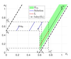
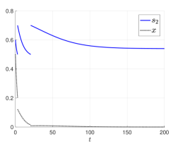
Figure 3. If $x(0)\leq X(s_{1}(0),s_{2}(0))$, then only finitely many impulses occur. The orbit converges, indicated by $\square$, after a finite number of impulses, and the $x$-component of the solution tends to $0$ as $t\to\infty$. The parameters are the values given in Example 1, and the initial condition is $(s_{1}(0),s_{2}(0),x(0))=(0.23,0.6,0.5)$.

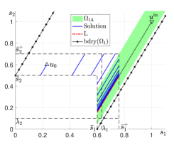
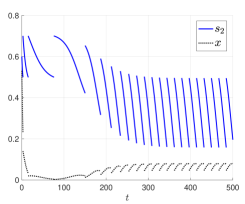
Figure 4. If $L$ lies in $\Omega_{1A}$ and $x(0)>X(s_{1}(0),s_{2}(0))$, then the solution converges to the periodic orbit. The parameters are the values given in Example 1, and the initial condition is $(s_{1}(0),s_{2}(0),x(0))=(0.23,0.6,0.53)$.

In the following Corollary, we consider a case in which we are guaranteed that $X(s_{1}^{0},s_{2}^{0})\leq 0$. In this case, by Proposition 4.12, it follows that any solution of (1) with $(s_{1}(0),s_{2}(0))=\Omega_{1}$ and $x(0)>0$ converges to the periodic orbit.

If $\bar{s}_{1}>\lambda_{1}$ and $\bar{s}_{2}>\lambda_{2}$, we define $\Omega_{\lambda}$ to be the region in the $s_{1}$-$s_{2}$ plane that lies between the lines $s_{2}=\bar{s}_{2}+R_{21}(s_{1}-\lambda_{1})$ and $s_{2}=\lambda_{2}+R_{21}(s_{1}-\bar{s}_{1})$ and above or to the left of $\Gamma^{-}$, i.e.,

$$\Omega_{\lambda}=\left\{(s_{1},s_{2}):\begin{aligned} &s_{1}>\bar{s}_{1}\;\text{or}\;s_{2}>\bar{s}_{2},\;\text{and}\\ &V(\lambda_{1},\bar{s}_{2})\leq V(s_{1},s_{2})\leq V(\bar{s}_{1},\lambda_{2})\end{aligned}\right\}.$$ (27)

For every $(s_{1},s_{2})\in\Omega_{\lambda}$, we have $\min\{f_{1}(s_{1}),f_{2}(s_{2})\}>D$, and so growth of $x$ is always positive in this region.

Corollary 4.15.

Assume $(s_{1}^{\mathrm{in}},s_{2}^{\mathrm{in}})\in\Omega_{1}$ and $\mu(r)>0$. If $\bar{s}_{1}>\lambda_{1}$ and $\widetilde{s}_{2}\geq\lambda_{2}$, then any solution $(s_{1}(t),s_{2}(t),x(t))$ with $(s_{1}(0),s_{2}(0))\in\Omega_{\lambda}$ and $x(0)>0$ converges to the unique periodic orbit of (1).

Proof.

First note that, since $\widetilde{s}_{2}\geq\lambda_{2}$, the line through $(\bar{s}_{1}^{+},\bar{s}_{2}^{+})$ is in $\Omega_{\lambda}$, and $\Omega_{\lambda}\cup\Omega_{1A}$ is connected. For any $(s_{1}^{0},s_{2}^{0})\in\Omega_{\lambda}$, we have $I(s_{1}^{0},s_{2}^{0})>0$ and $(g\circ\pi^{-})(s_{1}^{0},s_{2}^{0})\in\Omega_{\lambda}\cup\Omega_{1A}$. By (26), $X(s_{1}^{0},s_{2}^{0})<0<x(0)$, and by Theorem 4.14, $(s_{1}(t),s_{2}(t),x(t))$ converges to the periodic orbit. ∎

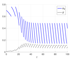
Figure 5. If $u_{0}\in\Omega_{\lambda}\setminus\Omega_{1A}$ and $\Omega_{\lambda}\cup\Omega_{1A}$ is connected, when $X(s_{1}^{0},s_{2}^{0})\leq 0$, the fermentation is still always successful for all $x(0)>0$. The parameters are the values given in Example 2. The initial condition is $(s_{1}(0),s_{2}(0),x(0))=(0.6,0.7,0.01)$.

Example 2.

Consider (1) with the Monod functional responses $f_{i}(s_{i})=\frac{m_{i}s_{i}}{a_{i}+s_{i}}$, $i=1,2$, and parameters $(m_{1},m_{2},a_{1},a_{2})=(2,2,1.4,0.6)$, $(Y_{1},Y_{2},D)=(2,0.7,0.5)$, and $(\bar{s}_{1},\bar{s}_{2},s_{1}^{\mathrm{in}},s_{2}^{\mathrm{in}},r)=(0.7,0.6,1,1,0.4)$. Then,

$$(\bar{s}_{1}^{+},\bar{s}_{2}^{+})=(0.82,0.76),\;\widetilde{s}_{2}\approx 0.42,\;\widehat{s}_{2}\approx 0.14,\;\mu(r)\approx 0.04,\;V_{-}\approx-0.19.$$

The equation $f_{i}(s_{i})=D$, $i=1,2$, yields $\lambda_{i}=\frac{a_{i}D}{D-m_{i}}$, which gives $\lambda_{1}\approx 0.4677$ and $\lambda_{2}=0.2$. Since $\lambda_{1}<\bar{s}_{1}$ and $\lambda_{2}<\widetilde{s}_{2}$, $\Omega_{\lambda}\cup\Omega_{1A}$ is a connected set, and the hypotheses in Corollary 4.15 are satisfied.

We take the initial value $(s_{1}^{0},s_{2}^{0})=(0.6,0.7)$. Then, $V(s_{1}^{0},s_{2}^{0})=-0.59$. A direct calculation gives $V(\lambda_{1},\bar{s}_{2})\approx-0.79$, so that $V(\lambda_{1},\bar{s}_{2})<V(s_{1}^{0},s_{2}^{0})<0$. This implies that $(s_{1}^{0},s_{2}^{0})\in\Omega_{\lambda}$. By Corollary 4.15, the fermentation succeeds for every initial value $x(0)>0$. An illustration is shown in Figure 5.

Remark 4.16.

If $\lambda_{2}>\widetilde{s}_{2}$ then the set $\Omega_{1A}\cup\Omega_{\lambda}$ is not connected. Then for some $(s_{1}^{0},s_{2}^{0})\in\Omega_{\lambda}$, $(g\circ\pi^{-})(s_{1}^{0},s_{2}^{0})$ is in the gap between $\Omega_{\lambda}$ and $\Omega_{1A}$. We are unable to rule out the possibility that the net growth in this gap is negative, and so it is conceiveable that $I((g\circ\pi^{-})(s_{1}^{0},s_{2}^{0}))<0$. In particular, we can choose $(s_{1}^{0},s_{2}^{0})\in\Omega_{\lambda}$ such that $I(s_{1}^{0},s_{2}^{0})<-I((g\circ\pi^{-})(s_{1}^{0},s_{2}^{0}))$. Therefore,

$$X(s_{1}^{0},s_{2}^{0})\geq-I(s_{1}^{0},s_{2}^{0})-(1-r)^{-1}I((g\circ\pi^{-})(s_{1}^{0},s_{2}^{0}))>0.$$ (28)

Therefore, for some positive initial concentrations of biomass, the reactor will fail, even though the initial conditions are in $\Omega_{\lambda}$.

5. Maximizing the Output

In this section we regard $r$ as a variable in the interval $(r_{*},1)$, where $r_{*}$ is the number given in Theorem 4.6.

For each $r\in(r_{*},1)$, there is a periodic orbit. In each period, there is exactly one impulse. As shown in the proof of Theorem 4.6, the left and right limits at an impulse are, respectively,

$$(\bar{s}_{1},\widehat{s}_{2},x_{-}(r))\quad\text{and}\quad(\bar{s}_{1}^{+}(r),\widehat{s}_{2}^{+}(r),x_{+}(r)),$$

where

$$x_{-}(r)=\frac{1}{r}\mu(r)\quad\text{and}\quad x_{+}(r)=\frac{1-r}{r}\mu(r).$$ (29)

The trajectory of the periodic orbit can be parametrized by

$$s_{2}=\widehat{s}_{2}+R_{21}(s_{1}-\bar{s}_{1})$$

and

$$x=X(s_{1};r) =x_{-}(r)-Y_{1}\int_{\bar{s}_{1}}^{s_{1}}1-\frac{D}{\min\big{\{}f_{1}(v),f_{2}(\widehat{s}_{2}+R_{21}(v-\bar{s}_{1}))\big{\}}}\;dv$$ (30)

$$=x_{+}(r)+Y_{1}\int_{s_{1}}^{\bar{s}_{1}^{+}}1-\frac{D}{\min\big{\{}f_{1}(v),f_{2}(\widehat{s}_{2}+R_{21}(v-\bar{s}_{1}))\big{\}}}\;dv$$ (31)

with $s_{1}\in(\bar{s}_{1},\bar{s}_{1}^{+})$ and $\bar{s}_{1}^{+}=\bar{s}_{1}+r(s_{1}^{\mathrm{in}}-\bar{s}_{1})$.

Denote the minimal period of the periodic orbit by $T(r)$. Then

$$T(r)=Y_{1}\int_{\bar{s}_{1}}^{\bar{s}_{1}^{+}(r)}\frac{1}{\min\big{\{}f_{1}(v),f_{2}(\widehat{s}_{2}+R_{21}(v-\bar{s}_{1}))\big{\}}\;X(v;r)}dv.$$ (32)

In the long run, the average amount of output divided by the total volume is

$$Q(r)=\frac{r}{T(r)}.$$

Maximizing $Q(r)$ for $r\in(r_{*},1)$ is equivalent to maximizing the output.

Lemma 5.1.

The minimal period $T(r)$, $r\in(r_{*},1)$ of the periodic orbit of (1) satisfies $\lim_{r\to 1^{-}}T(r)=\infty$. Also $\lim_{r\to r_{*}}T(r)=\infty$ if $r_{*}>0$.

Proof.

As $r\to 1$, we have $x_{+}(r)\to 0$. By (32) and (31), $T(r)\to\infty$.

If $r_{*}>0$, then by (29), $x_{-}(r)\to 0$ as $r\to r_{*}$. Along the periodic orbit, $x\geq x_{-}(r)>0$ and

$$\min\{f_{1}(s_{1}),f_{2}(s_{2})\}\geq\min\{f_{1}(\bar{s}_{1}),f_{2}(\bar{s}_{2})\}>0.$$

By (32) we conclude that $T(r)\to\infty$ as $r\to r_{*}$. ∎

Proposition 5.2.

The function $Q(r)=r/T(r)$, $r\in(r_{*},1)$, satisfies $\lim_{r\to 1}Q(r)=0$. If $r_{*}>0$, then $\lim_{r\to r_{*}}Q(r)=0$. If $r_{*}=0$, $\bar{s}_{1}\geq\lambda_{1}$, and $\widehat{s}_{2}\geq\lambda_{2}$, then $\lim_{r\to r_{*}}Q(r)=\min\{f_{1}(\bar{s}_{1}),f_{2}(\widehat{s}_{2})\}-D\geq 0$.

Proof.

By Lemma 5.1, $\lim_{r\to 1}Q(r)=1/(\lim_{r\to 1}T(r))=0$.

If $r_{*}>0$, then, by Lemma 5.1, $\lim_{r\to r_{*}}Q(r)=r_{*}/(\lim_{r\to r_{*}}T(r))=0$.

Next we assume $r_{*}=0$. By (32)

$$Q(r)=r\left/\left(Y_{1}\int_{\bar{s}_{1}}^{\bar{s}_{1}^{+}(r)}\frac{1}{\min\big{\{}f_{1}(v),f_{2}(\widehat{s}_{2}+R_{21}(v-\bar{s}_{1}))\big{\}}\;X(v;r)}\;dv\right)\right.,$$ (33)

where $X$ is defined by (30). Since $X(\bar{s}_{1};r)=x_{-}(r)=\frac{\mu(r)}{r}$, using L’Hôpital’s rule and the definition of $\mu(r)$ in (16),

$$\lim_{r\to 0}X(\bar{s}_{1};r)=Y_{1}\left.\frac{d\bar{s}_{1}^{+}(r)}{dr}\right|_{r=0}\left(1-\frac{D}{\min\{f_{1}(\bar{s}_{1}),f_{2}(\widehat{s}_{2})\}}\right).$$

Since $\bar{s}_{1}^{+}=\bar{s}_{1}+r(s_{1}^{\mathrm{in}}-\bar{s}_{1})$, we have

$$\left.\frac{d\bar{s}_{1}^{+}(r)}{dr}\right|_{r=0}=s_{1}^{\mathrm{in}}-\bar{s}_{1},$$ (34)

and it follows that

$$\lim_{r\to 0}X(\bar{s}_{1};r)=Y_{1}(s_{1}^{\mathrm{in}}-\bar{s}_{1})\left(1-\frac{D}{\min\{f_{1}(\bar{s}_{1}),f_{2}(\widehat{s}_{2})\}}\right).$$ (35)

Furthermore, we have

$$T^{\prime}(r)= \frac{Y_{1}(s_{1}^{\mathrm{in}}-\bar{s}_{1})}{\min\big{\{}f_{1}(\bar{s}_{1}^{+}),f_{2}(\widehat{s}_{2}+rR_{21}(s_{1}^{\mathrm{in}}-\bar{s}_{1}))\big{\}}\;X(\bar{s}_{1}^{+};r)}$$

$$-\frac{Y_{1}}{r^{2}}\int_{\bar{s}_{1}}^{\bar{s}_{1}^{+}(r)}\frac{\mu^{\prime}(r)r-\mu(r)}{\min\big{\{}f_{1}(v),f_{2}(\widehat{s}_{2}+R_{21}(v-\bar{s}_{1}))\big{\}}\;X(v;r)^{2}}dv.$$ (36)

Since $\bar{s}_{1}^{+}(0)=\bar{s}$ and $X(\bar{s}_{1};0)\neq 0$, by (35) and (36) we obtain

$$T^{\prime}(0)=\frac{Y_{1}(s_{1}^{\mathrm{in}}-\bar{s}_{1})}{\min\big{\{}f_{1}(\bar{s}_{1}),f_{2}(\widehat{s}_{2})\big{\}}\;X(\bar{s}_{1};0)}=\frac{1}{\min\{f_{1}(\bar{s}_{1}),f_{2}(\widehat{s}_{2})\}-D}.$$

From the expression $Q(r)=r/T(r)$, using L’Hôpital’s rule, we conclude that $\lim_{r\to 0}Q(r)=1/T^{\prime}(0)=\min\{f_{1}(\bar{s}_{1}),f_{2}(\widehat{s}_{2})\}-D$. ∎

Assume $r_{*}>0$. Since $\lim_{r\to r_{*}}Q(r)=\lim_{r\to 1}Q(r)=0$, by Proposition 5.2, $Q(r)$ attains its maximum at some value of $r$ in $(r_{*},1)$. Unfortunately, the analytical expression of the derivative $\frac{d}{dr}Q(r)$ is too complicated for finding a critical point of $Q(r)$. We have only obtained the maximum value using a numerical simulation. An illustration of the maximal value of $Q(r)$ is given in Figure 6.

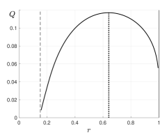
(A)	(B)

Figure 6. (A) $T(r)$ is the minimal period of the periodic orbit, $r\in(r_{*},1)$. The dashed line is $r=r_{*}$. As $r\to r_{*}$ or $r\to 1$, $T(r)\to\infty$. (B) The maximum of $Q(r)$ is attained at $r\approx 0.6416$, indicated by the dotted line. In the simulation, the response functions are $f_{i}(s_{i})=\frac{m_{i}s_{i}}{a_{i}+s_{i}}$, $i=1,2$, with parameters given in Example 2.

6. Discussion

We have modeled the self-cycling fermentation process assuming that there are two essential resources $s_{1}$ and $s_{2}$ that are growth limiting for a population of microorganisms, $x$, using a system of impulsive differential equations with state-dependent impulses. Assuming that the process is used for an application such as water purification, where the resources $s_{1}$ and $s_{2}$ are the pollutants, we assume that the threshold for emptying and refilling a fraction of the contents of the fermentor, resulting in the release of treated water, occurs when the concentrations of both pollutants reach an acceptable concentration set by some governmental agency. We called these thresholds, $s_{1}\leq\bar{s}_{1}$ and $s_{2}\leq\bar{s}_{2}$. We consider the process successful if once initiated, it proceeds indefinitely without a need for any subsequent interventions by the operator.

By solving the associated ODE system for $s_{2}$ in terms of $s_{1}$, we show that solutions, when projected onto the $s_{1}$-$s_{2}$ plane, are lines with slope given by the ratio of the growth yield constants. In order to derive necessary conditions for successful operation of the fermentor, we first divide the $s_{1}$-$s_{2}$ plane into two regions: $\Omega_{0}$ and $\Omega_{1}$. The model predicts that solutions of the associated system of ODEs with initial conditions in $\Omega_{0}$ approach the axes without ever reaching the thresholds for emptying and refilling and the reactor fails, independent of the initial concentration of microorganisms. Solutions of the associated system of ODEs with initial conditions in $\Omega_{1}$ have the potential to reach the threshold for emptying and refilling, but in this case, successful operation can also depend on the initial concentration of the population of microorganisms.

In most cases, at startup the input concentration of the pollutant would be the concentration of the pollutant in the environment, which we are assuming is constant, i.e., $(s_{1}(0),s_{2}(0))=(s_{1}^{\mathrm{in}},s_{2}^{\mathrm{in}})$. If, for any solution starting at these input concentrations of the resources, $(s_{1}^{\mathrm{in}},s_{2}^{\mathrm{in}})$, and positive concentration of biomass, $x(0)>0$, the threshold for emptying and refilling, $s_{1}\leq\bar{s}_{1}$ and $s_{2}\leq\bar{s}_{2}$, is reached with net positive growth of the biomass, the model analysis predicts that we can choose an emptying/refilling fraction, $r$, so that the system cycles indefinitely. In this case the solution approaches a periodic solution with one impulse per period.

If the system has a periodic solution, the $(s_{1},s_{2})$ components of the periodic orbit lie along the line with slope given by the ratio of the growth yield constants joining $(s_{1}^{\mathrm{in}},s_{2}^{\mathrm{in}})$ and the point in the $s_{1}$-$s_{2}$ plane where both thresholds are reached. The net change in the biomass on the periodic orbit, that we denote $\mu(r)$, must then also be positive.

For other initial conditions in $\Omega_{1}$, in order for the process to operate successfully, it is not enough that $\mu(r)>0$. There is also a minimum concentration of biomass, $X$, that depends on the initial concentration of the resources, that is required for the reactor to be successful. If the initial concentration of biomass is larger than $X$, then our analysis predicts that the reactor will cycle indefinitely and solutions will converge to the periodic orbit. If the initial concentration of biomass is less than or equal to $X$, then the reactor will cycle a finite number of times and then fail. If there is no periodic orbit, then the reactor will either cycle a finite number of times and then fail, or will cycle indefinitely, but the time between cycles will approach infinity.

Besides depending on the initial concentration of the resources at start up, the minimum concentration of biomass at startup required for successful operation depends on the emptying/refilling fraction in an interesting way. The closer $r$ is to one, the smaller the number of impulses that are required for solutions to get to the periodic orbit. However, the time spent in a region of negative growth could be larger, and so $X$ would be larger. The closer $r$ is to zero, results in less time spent in regions with negative growth, but more impulses are then required to get close to the periodic orbit. Each impulse removes biomass from the reactor, and so $X$ would also increase. This implies that there is an optimal value of $r$ for which the reactor has the best potential for success. The values of the growth yield constants, $Y_{1}$ and $Y_{2}$, also play a role in the size of $X$. If their ratio is held constant, but each value is scaled by a constant $c>0$, then $X$ is also scaled by the same constant $c$. Knowing this is important when selecting the population of microorganisms to use in the process.

If the choice of potential microorganisms for use in the process is restricted, then it might be easier to treat more highly polluted water than less polluted water, provided the microorganisms are not inhibited at high concentrations of the pollutant. We have shown that for successful operation, it is necessary that an $r$ exists such that $\mu(r)>0$. One way to increase $\mu(r)$ without changing anything else is to increase $s_{1}^{\mathrm{in}}$ and $s_{2}^{\mathrm{in}}$ in such a way that it still lies on the same line as before. It is also important to choose a population of microorganisms so that $(s_{1}^{\mathrm{in}}$,$s_{2}^{\mathrm{in}})$ lies in $\Omega_{1}$. It might only be possible to do this by increasing the concentration of one of the pollutants. However, another possibility might be to pre-process the input with a different population of microorganisms that moves $(s_{1}^{\mathrm{in}}$,$s_{2}^{\mathrm{in}})$ into an acceptable position so that a second population can then treat the water effectively.

We also make what might appear to be other surprising observations. Although the break-even concentrations play a role, it is not necessary for both break-even concentrations to be below their respective thresholds for emptying and refilling for the process to be successful (see Figure 4). Also, the process can still fail when both break-even concentrations are below their respective thresholds (see Figure 2).

For growth on a single, non-inhibitory, limiting resource in the self-cycling fermentation process, it has been shown that when the system has a periodic orbit, every solution either converges to the periodic orbit, or converges to an equilibrium without a single impulse [19]. If the resource is inhibitory at high concentrations, it has been shown that solutions may also converge to an equilibrium after a single impulse, but if there are at least two impulses then the solution is destined to converge to the periodic orbit[7]. In contrast, if there are two limiting essential resources, we have shown that there may be many impulses before the system converges to an equilibrium, even when the system has a periodic orbit. The example in Figure 3 demonstrates failure after two impulses.

An important issue when setting up the self cycling fermentation process is the choice of the emptying and refilling fraction, $r$. In the application we considered we were interested in optimizing the total amount of output. In the example, shown in section 5, we demonstrated that the optimal value of the emptying/refilling fraction is $r\approx 0.64$. This result is consistent with what was shown in the single resource cases [7, 19]. Another reason for implementing a self-cycling fermentation process instead of a continuous input process is to maximize the concentration of some microorganism in the output over some time period. For example, one recent ‘proof of concept’ study [23] investigated using the self-cycling fermentation process to improve the production of cellulosic ethanol production. In their investigation, and many other applications of self-cycling fermentation the emptying/refilling fraction $r$ is set to one half. While this is convenient for experiments and measurements, our results indicate that this is might not be the optimal choice of $r$.

REFERENCES

- [1] D. D. Baĭnov and P. S. Simeonov. Systems with impulse effect. Ellis Horwood Series: Mathematics and its Applications. Ellis Horwood Ltd., Chichester; Halsted Press [John Wiley & Sons, Inc.], New York, 1989. Stability, theory and applications.
- [2] D. D. Baĭnov and P. S. Simeonov. Impulsive differential equations: periodic solutions and applications, volume 66 of Pitman Monographs and Surveys in Pure and Applied Mathematics. Longman Scientific & Technical, Harlow; copublished in the United States with John Wiley & Sons, Inc., New York, 1993.
- [3] D. D. Baĭnov and P. S. Simeonov. Impulsive differential equations, volume 28 of Series on Advances in Mathematics for Applied Sciences. World Scientific Publishing Co., Inc., River Edge, NJ, 1995. Asymptotic properties of the solutions, Translated from the Bulgarian manuscript by V. Covachev [V. Khr. Kovachev].
- [4] G. Butler and G. S. K. Wolkowicz. Exploitative competition in a chemostat for two complementary, and possibly inhibitory, resources. Mathematical biosciences, 83:1–48, 1987.
- [5] A. Cinar, S. J. Parulekar, C. Ündey, and G. Birol. Batch fermentors, modeling,monitoring,and control. Marcel Dekker, New York, 2003.
- [6] F. Córdovea-Lepe, R. D. Valle, and G. Robledo. Stability analysis of a self-cycling fermentation model with state-dependent impulses. Mathematical methods in the applied sciences, 37:1460–1475, 2014.
- [7] G. Fan and G. S. K. Wolkowicz. Analysis of a model of nutrient driven self-cycling fermentation allowing unimodal response functions. Discrete and continuous dynamical systems, 8(4):801–831, 2007.
- [8] J. P. Grover. Resource competition. Population and community biology series 19. Chapman and Hall, New York, 1997.
- [9] A. Halanay and D. Wexler. Teoria calitativa a sistemelor du impulsuri. Ed. Acad. RSR, Bucharedt, 1968.
- [10] S. Hughes and D. Cooper. Biodegradation of phenol using the self-cycling fermentation process. Biotechnology and Bioengineering, 51:112–119, 1996.
- [11] J. A. León and D. B. Tumpson. Competition between two species for two complementary or substitutable resources. J. Theor. Biol., 50:185–2012, 1975.
- [12] B. Li, G. S. K. Wolkowicz, and Y. Kuang. Global asymptotic behavior of a chemostat model with two perfectly complementary resources with distributed delay. SIAM J. Appl. math., 60(6):2058–2086, 2000.
- [13] MATLAB. version 9.3.0 (R2017b). The MathWorks Inc., Natick, Massachusetts, 2017.
- [14] L. Perko. Differential equations and dynamical systems. Springer-Verlag, 1996.
- [15] A. Samoilenko and N. Perestyuk. Impulsive differential equations. World Scientific, Singapore, 1995.
- [16] B. E. Sarkas and D. G. Cooper. Biodegradation of aromatic compounds in a self-cycling fermenter. The Canadian Journal of Chemical Engineering, 72(5):874–880, 1994.
- [17] D. Sauvageau, Z. Storms, and D. G. Cooper. Sychronized populations of Escherichia coli using simplified self-cycling fermentation. Journal of Biotechnology, 149:67–73, 2010.
- [18] H. L. Smith and P. Waltman. The theory of the chemostat, volume 13 of Cambridge Studies in Mathematical Biology. Cambridge University Press, Cambridge, 1995. Dynamics of microbial competition.
- [19] R. J. Smith and G. S. K. Wolkowicz. Analysis of a model of the nutrient driven self-cycling fermentation process. Dynamics of continuous, discrete and impulsive systems, 11:239–265, 2004.
- [20] Z. J. Storms, T. Brown, D. Sauvageau, and D. G. Cooper. Self-cycling operation increases productivity of recombinent protein in Escherichia Coli. Biotechnology and Bioengineering, 109(9):2262–2270, 2012.
- [21] D. Tilman. Resource competition and community structure. Princeton University Press, New Jersey, 1982.
- [22] J. Von Liebig. Die organische Chemie in ihrer Anwendung auf Agrikultur und Physiologie. Friedrich Vieweg, Braunschweig, 1840.
- [23] J. Wang, M. Chae, D. Sauvageau, and D. C. Bressler. Improving ethanol productivity through self-cycling fermentation of yeast: a proof of concept. Biotechnology for biofuels, 10(1):193, 2017.
- [24] J. Wu, H. Nie, and G. S. K. Wolkowicz. A mathematical model of competition for two essential resources in the unstirred chemostat. SIAM J. Appl. Math., 65:209–229, 2004.