The Influence of H2O Pressure Broadening in High Metallicity Exoplanet Atmospheres

Abstract

Planet formation models suggest broad compositional diversity in the sub-Neptune/super-Earth regime, with a high likelihood for large atmospheric metal content ($\geq$ 100 $\times$ Solar). With this comes the prevalence of numerous plausible bulk atmospheric constituents including N2, CO2, H2O, CO, and CH4. Given this compositional diversity there is a critical need to investigate the influence of the background gas on the broadening of the molecular absorption cross-sections and the subsequent influence on observed spectra. This broadening can become significant and the common H2/He or “air” broadening assumptions are no longer appropriate. In this work we investigate the role of water self-broadening on the emission and transmission spectra as well as on the vertical energy balance in representative sub-Neptune/super-Earth atmospheres. We find that the choice of the broadener species can result in a 10 – 100 parts-per-million difference in the observed transmission and emission spectra and can significantly alter the 1-dimensional vertical temperature structure of the atmosphere. Choosing the correct background broadener is critical to the proper modeling and interpretation of transit spectra observations in high metallicity regimes, especially in the era of higher precision telescopes such as JWST.

1 Introduction

A primary goal of exoplanet science is the determination of basic planetary conditions. Transit spectrophotometry observations of planetary atmospheres offer a window into fundamental quantities such as climate and composition e.g Madhusudhan et al. (2016)). Determining atmospheric composition is a necessary requirement for assessing the relative importance of various chemical processes (Moses, 2014) and greatly assists in understanding planet formation by linking volatile inventory to proto-planetary disk processes (Öberg et al., 2011; Mordasini et al., 2016).

One of the key findings of the Kepler Mission (Borucki et al., 1997) is that a majority of exoplanets fall within this “warm sub-Neptune” regime ($\sim$2–4 Earth radii, T$<$1000 K ) (Fressin et al., 2013). These planets have been an intense area of focus for transit spectra observations with the Hubble Space Telescope (HST) (Kreidberg et al., 2014a; Fraine et al., 2014; Knutson et al., 2014) and will be over the next decade as they serve as the link between jovian worlds and terrestrial planets as well as being the most prolific population of planets to be found by the Transiting Exoplanet Explorer Satellite (TESS, (Sullivan et al., 2015; Louie et al., 2018; Barclay et al., 2018; Kempton et al., 2018)).

Planet formation, interior structure, and atmospheric chemistry modeling (Fortney et al., 2013; Moses et al., 2013; Lopez & Fortney, 2014) suggest extreme compositional diversity within this sub-population, with a high likelihood for large atmospheric metallicities (¿300$\times$ Solar). Given this potential for compositional diversity, the assumption of “jovian-like” H2/He-dominated atmospheres may not always be appropriate. Instead, with currently measured atmospheric metallicities reaching as high as $\sim$300-1000$\times$ solar (Line et al., 2014; Fraine et al., 2014; Kreidberg et al., 2014b; Knutson et al., 2014; Morley et al., 2017), molecules such as H2O and CO2 will become the dominant bulk constituents (Moses et al., 2013; Hu & Seager, 2014).

Along with this diversity in composition, comes with it numerous challenges in atmospheric modeling ranging from chemical modeling (Hu & Seager, 2014) to cloud microphysics (Ohno & Okuzumi, 2018) to 3D climate modeling (Kataria et al., 2014). Nearly all flavors of atmospheric modeling that aim to make observational predictions necessarily require radiative transfer computations. A key necessary ingredient in radiative transfer computations is the opacities, which for planets, are dominated by the molecular absorption cross-sections (hereafter, ACS). The ACS of a given molecule typically consist of billions of lines representing the ability of a molecule to absorb or emit photons. Each line has its own line-width (or broadening) typically specified through the degree of thermal/Doppler and pressure broadening (Goody & Yung, 1995). Pressure broadening is the net cumulative effect of interactions between the absorbing molecule in question (e.g., H2O) with its neighboring molecules (or bath gases, e.g., H2, He) or by self-broadening (H2O with itself). Much exo-atmospheric relevant ACS focus, specifically broadening, has been jovian-centric (e.g., H2$/$He dominated compositions and broadening Freedman et al. (2008); Tennyson et al. (2016); Grimm & Heng (2015); Hedges & Madhusudhan (2016)) being largely driven by the abundance of high fidelity “hot-Jupiter” observations and carry over from brown dwarf modeling.

Exploration of pressure broadening assumptions in exo-atmospheres is not new (e.g., Grimm & Heng (2015); Hedges & Madhusudhan (2016)). Hedges & Madhusudhan (2016) provide a comprehensive overview of the various pressure broadening effects including resolution, line-wing cutoff, Doppler vs. pressure, and more relevant to our investigation, an initial look at the impact of a broadener choice. They too explore the impact of H2O vs H2 broadening on the H2O ACS, specifically over HST wavelengths, and find that the band-averaged ACS can change by up to an order-of-magnitude.

In this letter we expand upon the work in Hedges & Madhusudhan (2016) to not only determine the influence of H2O self-broadening on the H2O ACS, but also as a function of water fraction, and more importantly we quantitatively assess the integrated effect that the broadener choice has on the observable spectra as well as on the impact on atmospheric vertical energy balance. This work is crucial to the proper interpretation of transit spectra observations in high metallicity regimes, expected of the sub-Neptune/Super-Earth population. In §2 we describe our data sources and how we compute the ACS and the transmission/emission spectrum and self-consistent modeling approach. In §3 we compare the impact of H2O self-broadening with the standard H2/He broadening assumption. Finally, in §4 we discuss the implications and future prospects. We also make our newly computed water ACS grid for both broadeners publically available.

2 Methods

In this initial investigation on the impact of non H2/He foreign broadening on transmission/emission spectra, we choose to focus on H2O because: 1) H2O is the most prominent absorber in exoplanet spectra due to its large abundance over a range of elemental compositions (Moses et al., 2013) and multiple strong absorption bands from the optical to far infrared wavelengths and 2) it shows the largest sensitivity to choice of broadener when compared to other species (a factor of $\sim$7 increase in broadening when compared to H2/He, Table 1).

Table 1: Lorentzian half-width coefficients $\gamma_{L}$ [cm^-1/bar]^∗,† for relevant broadeners. The focus of this work is on influence H₂O self and H₂/He broadening on the H₂O absorption cross-sections (bold).

Absorber	Broadener	$\gamma_{L}$	$relative$ $to$ $\gamma_{L}^{H_{2}/He}$
H2O	Self ‡	0.3 – 0.54	7$\times$
	H2/He ¶	0.05 – 0.08	1$\times$
	CO2	0.15 – 0.20	3$\times$
	air	0.08 – 0.1	1.5$\times$
CH4	Self	0.06 – 0.09	1.5$\times$
	H2/He	0.05 – 0.08	1$\times$
	H2O	0.06 – 0.09	1.5$\times$
	CO2	0.07 – 0.09	1.5$\times$
	air	0.02 – 0.07	1$\times$
CO2	Self	0.08 – 0.12	2$\times$
	H2/He	0.09 – 0.12	2$\times$
	H2O	0.10 – 0.14	2.5$\times$
	air	0.05 – 0.08	1$\times$
CO	Self	0.04 – 0.09	1$\times$
	H2/He	0.04 – 0.08	1$\times$
	H2O	0.07 – 0.1	1.5$\times$
	CO2	0.09 – 0.1	1.5$\times$
	air	0.05 – 0.07	1$\times$

^∗ The pressure broadening/Lorentzian line profile is defined with a half-width $\Gamma_{L}$ = $(T/296)$ ${}^{-n_{T}}$ $\sum_{b}$ $\gamma_{L}^{b}$ $P_{b}$ where $\gamma_{L}^{b}$ is the Lorentzian coefficient for broadener, $b$, $P_{b}$ is the partial pressure of broadener $b$, and n_T is the thermal coefficient (typically 0.5 under kinetic theory).

^† Data extracted from Refs. in Table 3 of (Hartmann et al., 2018) and from (Gordon et al., 2017).

^‡ Denoted by H2O@[self] in the text and figures.

^¶ Denoted by H2O@[H2+He] in the text and figures.

The approach is to compute the H2O ACS under different end-member compositional scenarios, with the first the standard “jovian-like” H2/He broadening (H2O@[H2+He]) and the second, pure H2O broadening (H2O@[self]), which is more appropriate for high metallicity or all-steam atmospheres. We then determine the spectral differences between H2/He and self-broadening of H2O in representative atmospheres.

2.1 Computation of pressure-broadened H_2 ^16O absorption cross-section

Table 2: Grid and computational assumptions over which the H${}_{2}^{16}$O cross sections are computed. There are 270 T-P combinations and two broadener choices (H₂+He vs. H₂O). A variable wavenumber resolution is chosen to properly sample the Voigt-widths at each given T-P pair. Finer sampling results in negligible differences in the ACS.

ACS	Case	1:	85$\%$	H2	15$\%$	He
	Case	2:	100$\%$	H2O
T(K)	400	425	475	500	575	650	725	800
	900	1000	1100	1200	1300	1400	1500
P(bar)	10-6	3$\times$10-6	10-5	3$\times$10-5	10-4	3$\times$10-4
	10-3	3$\times$10-3	10-2	3$\times$10-2	10-1	3$\times$10-1
	1	3	10	30	100	300
Resolution∗		100	–	1000	cm-1	:	1/$\Gamma_{V}$
		1000	–	30000	cm-1	:	2/$\Gamma_{V}$
Line wing cut-off†			P$\geq$1	bar:	100	cm-1
			P$<$1	bar:	300	cm-1

^∗ $\Gamma_{V}$ is the Voigt half-width approximated as 0.5346$\Gamma_{L}+\sqrt{0.2166\Gamma_{L}^{2}+\Gamma_{G}^{2}}$, with $\Gamma_{G}$ the Doppler width (Olivero & Longbothum, 1977).

^† The Lorentz wing shape may not be appropriate out at such distances (Freedman et al., 2008)

We utilize the freely-available EXOMOL (Tennyson et al., 2016) line-list data (e.g., BT2 line list (Barton et al., 2017)) and EXOCROSS routine (Yurchenko et al., 2017) to compute the pressure-broadened H2O ACS database (Table 2) for two broadening scenarios: 1) 85$\%$ H2 and 15$\%$ He (current standard assumption) using the $J$-dependent pressure coefficients from EXOMOL (Barton et al., 2017), and 2) 100$\%$ H2O using the average value of available experimental self-broadening coefficients (Ptashnik et al., 2016).

2.2 Modeling the Impact on Transmission/Emission Spectra of Transiting Exoplanets

To assess the signifigance of the type-of-broadener assumption, we use the CHIMERA (Line et al., 2013, 2014; Stevenson et al., 2014; Kreidberg et al., 2015; Line & Parmentier, 2016; Kreidberg et al., 2018) code with our newly generated ACS (converted to $\lambda/\Delta\lambda$=100 correlated-K coefficients (Amundsen et al., 2016)) to model transit/eclipse spectra of a representative sub-Neptune like planet (GJ1214b (Harpsøe et al., 2013), T_eq=500–900K). We first generate forward model spectra using both sets of ACS (H2O@[self] and H2O@[H2+He]) given a fixed temperature-pressure profile (TP, Guillot (2010) Eqs. 24, 49 ) and either 100% H2O or 500$\times$Solar metallicity under thermochemical equilibrium. Second, we compute a self-consistent radiative equilibrium atmosphere (Arcangeli et al., 2018; Mansfield et al., 2018; Kreidberg et al., 2018) to determine the impact of water broadening on the vertical energy balance and, in turn, on the observed spectra. We discuss our findings in the next section.

3 Results

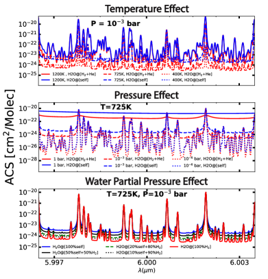
Figure 1: Illustration of the impact of @[self] (blue) versus @[H2+He] (red) on the absorption cross sections near 6$\mu$m. The top panel shows the influence of temperature on the broadening difference at a fixed represantative pressure of 1 mbar. At 1200K (1 mbar) the lines are purely Doppler broadened resulting in little effect. The middle panel shows the influence of pressure at a fixed temperature. The Doppler cores are negligible by 1 bar. The bottom panel shows the impact of the relative weighting of self versus H2 broadening (e.g., composition dependence) at a fixed temperature and pressure. Cross-section differences are largest in the pressure-broadened line wings, with pure @[self] typically 1 order of magnitude larger. A factor of 5 in broadening difference occurs by the time the relative abundance of water reaches $\sim$30%. In general, @[self] broadening becomes more important at higher pressures, cooler temperatures, and longer wavelengths due to the increased prominence of pressure broadening over Doppler broadening.

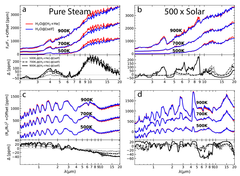
Figure 2: Effect of water self-broadening (@[self], blue) compared to the standard H2/He broadening (@[H2+He], red) on pure steam (left column: a,c) and high metallicity (500$\times$ solar-right column: b,d) atmospheres with equilibrium temperatures of 500, 700, and 900K. The top row (a,b) compares emission spectra and the bottom row shows relative transmission spectrum differences (c,d). The bottom panel in each shows the relative spectral difference ($\Delta$). Differences range anywhere from a few 10s to a few 100s of ppm and show a strong wavelength dependence.

3.1 Impact on Cross Sections

Figure 1 illustrates the effect of temperature, pressure, and water abundance on the difference between @[self] and @[H2+He] broadened ACS near 6 $\micron$. The top panel shows how broadening changes with temperature at a fixed pressure of 1 mbar. Differences are largest for cooler temperatures where pressure broadening becomes more important. The middle panel illustrates the impact of variable pressure at a fixed temperature (725K). Even at low pressures (1 $\mu$bar) pressure broadening differences are still present in the line wings. The bottom panel shows the effect of varying water abundance on the combined @[self]+@[H2] broadening at a fixed temperature and pressure (725K, 1 mbar). With pure self-broadening, differences in the line wings can approach an order of magnitude. For a $\sim$30% mole fraction of water, the ACS is about 3–5$\times$ greater than pure hydrogen broadening. While not shown, these differences become larger at longer wavelengths and smaller at shorter wavelengths due to the relative importance of Doppler-to-pressure broadening.

3.2 Direct Impact on Transmission/Emission Spectra

More practically, Figure 2 summarizes the key impact of @[H2+He] versus @[self] broadening on the emission (top row) and transmission (bottom row) spectra of a typical sub-Neptune under the assumption of a pure steam atmosphere (left column) and a 500$\times$Solar metallicity scenario (right column). Overall, we find that the differences are quite large, 10s to 100s of ppm, well within the detectable range of both HST (Kreidberg et al., 2014a), and certainly the James Webb Space Telescope (JWST, e.g., Greene et al. (2016); Bean et al. (2018)), especially for the anticipated windfall of such planets around bright stars (Sullivan et al., 2015).

In the all-steam atmospheres, emission differences (Figure 2a) are largest in the window regions ($\sim 4\mu$m, $\sim 10\mu$m ). The increased flux for the @[H2+He] broadened ACS is because of the lower opacity, permiting flux from deeper, hotter layers to emerge (for a fixed TP). The increased opacity due to the @[self] broadening obscures the deeper/hotter layers, resulting in lowered fluxes at those wavelengths. These differences are, of course, strongly dependent upon the temperature structure within in the atmosphere. As these spectra assume a fixed TP there is a difference in net radiated flux, which will most certainly have an influence on the radiative balance and thermal structure in the atmosphere, as discussed in §3.3.

Transmission spectra tell a similar, albeit less dramatic story with relative differences of $\sim$60 ppm across shown wavelength range. The “linear-like” slope in the differences ($\Delta$) with wavelength is due to the frequency dependence of Doppler-to-Pressure broadening.

The effects at high metallicity (500$\times$solar, Figure 2, right column) are less extreme (10 of ppm) due to the reduced abundance of H2O (10 – 20%) and the significant abundances of additional opacity sources (mainly CO2, CO, CH4, and H2/He). Furthermore, due to the reduced impact of H2O@[self] broadening (Figure 1), we expect an approximate (comparing 1 mbar line wings) reduction of 3–5$\times$ to $\sim<$ 10ppm in the transmission spectra.

3.3 Impact on Self-Consistent 1D Atmosphere

Figure 3 shows the impact of self-broadening on the 1D radiative balance (and subsequent observational effects) of a $\sim$550K planet under the all steam and 500$\times$Solar scenarios. The @[self] broadening results in $\sim$100-180K hotter temperatures below the $\sim$1 mbar level and $\sim$60Kcooler above for the all steam scenario (Figure 3a). More intuitively, the increased @[self] mean opacity “shifts” the averaged thermal “$\tau$=1” level to a $\sim 3\times$ lower pressure in the all steam scenario. This shift is readily seen in the band averaged contribution functions (Figure 3a). A similar, but lesser, effect is seen in the 500$\times$Solar metallicity scenario (up to $\sim$ 70 K) because the water abundance is lower by a factor of $\sim 5$ (Figure 3b). The radiative response of the TP to the integrated flux differences (up to 40% for steam and 10% for 500$\times$solar, green vs. red curves in Figure 3c,d ) between the @[self] vs. @[H2+He] acts to reduce the emission spectrum differences, however, to a still detectable 10s of ppm (Figure 3c,d).

The transmission spectra (Figure 3e,f) show comparable differences (30–40 ppm) to the 500 K scenario from Figure 2c,d. However, there are now two effects taking place that create the transmission differences. The first is the scale height effect due to the differences in the TP (@[H2+He]-@[self], H2O TP). The second, as before, is the broadening differences. Both effects contribute equally to the overall differences in the transmission spectra. Despite the self-consistent adjustment of the TP, differences in both emission and transmission are still above detectable levels (10s of ppm)

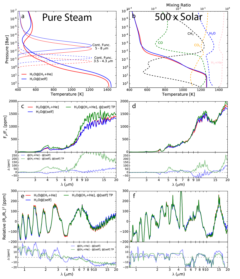
Figure 3: Comparison of the @[self] (blue) vs. @[H2+He] (red) broadening in self-consistent 1D thermochemical-radiatve-equilibrium atmospheres for all steam (left column: a,c,e) and 500$\times$solar (right column: b,d,f) composition. The top row (a,b) shows the derived radiative-equilibrium TP under each scenario. Thermal emission contribution functions averaged over represenative bands (Cont. Func. 5–8, and 3.5–4.3 $\mu$m) for each broadening scenario are shown in (a). Subplot (b) shows the thermochemical equilibrium mixing ratios along the @[self] TP for select species. Temperature differences can be up to 175K (20%) in the pure steam scenario and up to 70K in the 500$\times$Solar scenario. The second row (c,d) shows the resultant secondary eclipse spectra and their differences below ($\Delta$). An additional emission spectrum (@[H2+He], @[self] TP-green), is shown in (c) and (d) assuming the same TP as the @[self] scenario in order to decouple the effects of the radiatively adjusted TP from the broadening differences. The last row (e,f) shows the resulting cloud free transmission spectra and relative differences. An additional transmission spectrum (@[H2+He], @[self] TP-green), is shown in (e) and (f) assuming the same TP as the @[self] scenario in order to decouple the effects of the broadening and scale height change due to TP variation. Spectral differences are on the order of 30-40 ppm in transmission but are much less in emission ($\sim$60 ppm) when compared to Figure 2a,b due to the radiative adjustment of the TP.

4 Conclusions

The aim of this work was to determine the observable impact of broadener composition on observed transiting planet spectra, with application to $<1000$K high-metallicity and all steam atmospheres, likely representative of the sub-Neptune/Super-Earth population of planets. As a specific example, we focused on the difference between H2/He broadening and self broadening on the water absorption cross-sections as water is typically the most prevalent species and absorber in planetary atmospheres. From our analysis we arrive at the following key points:

• Absorption cross section differences between water self and the standard assumed H2/He broadening are up to an order of magnitude in the pressure broadened line wings (similar to Hedges & Madhusudhan (2016)), and is noticeable over a range of applicable temperatures and pressures.

• The influence of self-broadening is composition dependent and non-linear, with $\sim$half of the difference achieved by water mole fractions of$\sim$30% for a representative temperature and pressure.

• Transmission and emission spectra differences for representative sub-Neptune atmospheres range between a few 10s of ppm up to 100s of ppm, depending upon wavelength, temperature, and water abundance. These differences are not negligible considering currently achieved HST precisions of $\sim$15 ppm and possible precisions as low as a few ppm for JWST. Differences will vary depending upon additional parameters like temperature gradient (for emission), planet-to-star radius ratio, and scale height.

• The assumption of water self-broadening (or lack thereof) can have a significant impact on the 1D vertical energy balance, with temperature differences of up to 180K in pure steam atmospheres (or a half-a-decade lower pressure shift in the emission levels) and 10s of K in high metallicity atmospheres.

This work is certainly not an exhaustive exploration of all possible broadening (Table 1) or planetary atmosphere conditions. However, it serves to illustrate that the broadener assumption can have a non-negligible impact on the observables and continues to illustrate the importance and key role of laboratory data on planetary atmosphere modeling. (Fortney et al., 2016)

5 Acknowledgements

EGN and MRL thank J. Lyons, A. Heays, R. Freedman, M. Marley, J. Fortney, P. Mollière, and L. Pino for many useful discussions. We especially thank S. Yurchenko for invaluable assistance with the EXOCROSS code, and ASU Research Computing center for the kind support on computational side. MRL acknowledges summer support from the NASA Exoplanet Research Program award NNX17AB56G. This work benefited from numerous conversations at the 2018 Exoplanet Summer Program in the Other Worlds Laboratory (OWL) at the University of California, Santa Cruz, a program funded by the Heising-Simons Foundation.

References

- Amundsen et al. (2016) Amundsen, D. S., Mayne, N. J., Baraffe, I., et al. 2016, A & A, 595, A36
- Arcangeli et al. (2018) Arcangeli, J., Désert, J.-M., Line, M. R., et al. 2018, ApJ, 855, L30
- Barclay et al. (2018) Barclay, T., Pepper, J., & Quintana, E. V. 2018, ArXiv e-prints, arXiv:1804.05050
- Barton et al. (2017) Barton, E. J., Hill, C., Yurchenko, S. N., et al. 2017, JQSRT, 187, 453
- Bean et al. (2018) Bean, J. L., Stevenson, K. B., Batalha, N. M., et al. 2018, arXiv:1803.04985
- Borucki et al. (1997) Borucki, W. J., Koch, D. G., Dunham, E. W., & Jenkins, J. M. 1997, in ASP Conf. Ser., Vol. 119, Planets Beyond the Solar System and the Next Generation of Space Missions, ed. D. Soderblom, 153
- Fortney et al. (2013) Fortney, J. J., Mordasini, C., Nettelmann, N., et al. 2013, ApJ, 775, 80
- Fortney et al. (2016) Fortney, J. J., Robinson, T. D., Domagal-Goldman, S., et al. 2016, arXiv:1602.06305
- Fraine et al. (2014) Fraine, J., Deming, D., Benneke, B., et al. 2014, Nature, 513, 526
- Freedman et al. (2014) Freedman, R. S., Lustig-Yaeger, J., Fortney, J. J., et al. 2014, ApJS, 214, 25
- Freedman et al. (2008) Freedman, R. S., Marley, M. S., & Lodders, K. 2008, ApJS, 174, 504
- Fressin et al. (2013) Fressin, F., Torres, G., Charbonneau, D., et al. 2013, ApJ, 766, 81
- Goody & Yung (1995) Goody, R. M., & Yung, Y. L. 1995, Atmospheric Radiation : Theoretical Basis., 2nd edn. (Oxford University Press), 536
- Gordon et al. (2017) Gordon, I., Rothman, L., Hill, C., et al. 2017, JQSRT, 203, 3
- Gordon & Mcbride (1994) Gordon, S., & Mcbride, B. J. 1994, Technical Report
- Greene et al. (2016) Greene, T. P., Line, M. R., Montero, C., et al. 2016, ApJ, 817, 17
- Grimm & Heng (2015) Grimm, S. L., & Heng, K. 2015, ApJ, 808, 182
- Guillot (2010) Guillot, T. 2010, AA, 520, A27
- Harpsøe et al. (2013) Harpsøe, K. B. W., Hardis, S., Hinse, T. C., et al. 2013, A&A, 549, A10
- Hartmann et al. (2018) Hartmann, J.-M., Tran, H., Armante, R., et al. 2018, JQSRT, 213, 178
- Hedges & Madhusudhan (2016) Hedges, C., & Madhusudhan, N. 2016, MNRAS, 458, 1427
- Hu & Seager (2014) Hu, R., & Seager, S. 2014, ApJ, 784, 63
- Kataria et al. (2014) Kataria, T., Showman, A. P., Fortney, J. J., Marley, M. S., & Freedman, R. S. 2014, ApJ, 785, 92
- Kempton et al. (2018) Kempton, E. M.-R., Bean, J. L., Louie, D. R., et al. 2018, ArXiv e-prints, arXiv:1805.03671
- Knutson et al. (2014) Knutson, H. A., Benneke, B., Deming, D., & Homeier, D. 2014, Nature, 505, 66
- Kreidberg et al. (2018) Kreidberg, L., Line, M. R., Thorngren, D., Morley, C. V., & Stevenson, K. B. 2018, ApJ, 858, L6
- Kreidberg et al. (2014a) Kreidberg, L., Bean, J. L., Désert, J.-M., et al. 2014a, Nature, 505, 69
- Kreidberg et al. (2014b) Kreidberg, L., Bean, J. L., Désert, J. M., et al. 2014b, ApJL, 793, 2
- Kreidberg et al. (2015) Kreidberg, L., Line, M. R., Bean, J. L., et al. 2015, ApJ, 814, 66
- Line et al. (2013) Line, M. R., Knutson, H., Deming, D., Wilkins, A., & Desert, J.-M. 2013, ApJ, 778, 183
- Line et al. (2014) Line, M. R., Knutson, H., Wolf, A. S., & Yung, Y. L. 2014, ApJ, 783, 70
- Line & Parmentier (2016) Line, M. R., & Parmentier, V. 2016, ApJ, 820, 78
- Lodders et al. (2009) Lodders, K., Palme, H., & Gail, H.-P. 2009, 712–770
- Lopez & Fortney (2014) Lopez, E. D., & Fortney, J. J. 2014, ApJ, 792, 1
- Louie et al. (2018) Louie, D. R., Deming, D., Albert, L., et al. 2018, PASP, 130, 044401
- Madhusudhan et al. (2016) Madhusudhan, N., Agúndez, M., Moses, J. I., & Hu, Y. 2016, Space Sci. Rev., 205, 285
- Mansfield et al. (2018) Mansfield, M., Bean, J. L., Line, M. R., et al. 2018, AJ, 156, 10
- Mordasini et al. (2016) Mordasini, C., van Boekel, R., Mollière, P., Henning, T., & Benneke, B. 2016, ApJ, 832, 1
- Morley et al. (2017) Morley, C. V., Knutson, H., Line, M., et al. 2017, AJ, 153, 86
- Moses (2014) Moses, J. I. 2014, Phil. Trans. Roy. Soc. A, 372, 20130073
- Moses et al. (2013) Moses, J. I., Line, M. R., Visscher, C., et al. 2013, ApJ, 777, 34
- Öberg et al. (2011) Öberg, K. I., Murray-Clay, R., & Bergin, E. A. 2011, ApJ, 743, L16
- Ohno & Okuzumi (2018) Ohno, K., & Okuzumi, S. 2018, ApJ, 859, 34
- Olivero & Longbothum (1977) Olivero, J., & Longbothum, R. 1977, J. Quant. Spec. Radiat. Transf., 17, 233
- Ptashnik et al. (2016) Ptashnik, I. V., McPheat, R., Polyansky, O. L., Shine, K. P., & Smith, K. M. 2016, JQSRT, 177, 92
- Stevenson et al. (2014) Stevenson, K. B., Bean, J. L., Seifahrt, A., et al. 2014, AJ, 147, 161
- Sullivan et al. (2015) Sullivan, P. W., Winn, J. N., Berta-Thompson, Z. K., et al. 2015, ApJ, 809, 77
- Tennyson et al. (2016) Tennyson, J., Yurchenko, S. N., Al-Refaie, A. F., et al. 2016, JMS, 327, 73
- Yurchenko et al. (2017) Yurchenko, S. N., Tennyson, J., & Barton, E. J. 2017, J. Phys.: Conf. Ser., 810, 012010