Scattering with real-time path integrals

W. N. Polyzou, Ekaterina Nathanson

Proceedings for Few Body 22, Caen, France

• Abstract:Sharp-momentum transition matrix elements for scattering from a short-range Gaussian potential are computed using a real-time path integral. The computation is based on a numerical implementation of a new interpretation of the path integral as the expectation of a potential functional with respect to a complex probability distribution on cylinder sets of paths. The method is closely related to a unitary transfer matrix computation.

1 Path integrals and complex probabilities

Path integrals [1][2] provide a means for treating problems in quantum mechanics that are often difficult to treat by other means. Normally path integral calculations are limited to quadratic interactions or generating perturbation theory. When the time can be made imaginary they can also be approximated using Monte Carlo [3] integration.

Most applications are naturally formulated using real time. Scattering is one such application. While the computation of real-time path integrals is more challenging, it is interesting to explore how far real-time applications can be pushed. One motivation is because real-time path integrals represent unitary time evolution, direct treatments of real-time path integrals have the potential to be candidates for applications of quantum computing algorithms.

The problem with the interpretation of the real-time path integral as an integral is that the measure has to be additive on a countable union of disjoint measurable sets. When the measure is not positive, the evaluation of a countable sum of non-positive numbers can be both infinite or finite, depending on how it is evaluated.

In [4][5][6] the Feynman path integral is reinterpreted as the expectation of a potential functional

$$E[F]\qquad F[\gamma]:=e^{-i\int V(\gamma(t))dt}$$ (1)

with respect to a complex probability on a space of paths. It was shown in [5][6] that this interpretation results in a global solution of the Schrödinger equation.

Classical probabilities on the real line are defined on measurable sets that are generated by intervals under complements and countable unions. These sets are the Lebesgue measurable sets. A Probability is a non-negative Lebesgue measurable function that integrates to 1.

The Henstock-Kurzweil integral [7][8] provides an extension of the Lebesgue integral that is defined similar to a Riemann integral. Hesntock developed an alternative probability theory based on the this integral. Henstock’s probability agrees with classical probability theory when the probability is non-negative, however he realized that it could be extended to non-positive and complex probabilities if countable additivity was replaced by finite additivity. P. Muldowney [4] suggested that this interpretation could also be extended to reinterpret path integrals not as integrals, but as the expectation of a potential functional with respect to a complex probability distribution on a space of paths. Jørgensen and Nathanson verified that this interpretation leads to approximations that converge to global solutions of the Schrödinger equation.

In one dimension the path-integral representations of the unitary time evolution operator for a particle of mass $\mu$ in a potential $V$ can be expressed as:

$$\langle x_{0}|e^{-iHt}|\psi\rangle=$$

$$\lim_{N\to\infty}({\mu\over 2\pi i\Delta t})^{N/2}\int\prod_{i=n}^{N}dx_{n}e^{i{\mu\over 2\Delta t}(x_{n-1}-x_{n})^{2}-iV(x_{n})\Delta t}\langle x_{N}|\psi\rangle.$$ (2)

where $\Delta t:=t/N$. This follows from the Trotter product formula [9] and is the standard form of the path integral. It is expressed as the limit of $N$-dimensional integrals as $N\to\infty$.

The complex probability interpretation arises by expressing the real line as the union of a finite number of disjoint intervals

$$\mathbb{R}=\underbrace{(-\infty,x_{1n})}_{I_{0n}}\underbrace{[x_{1n},x_{2n})}_{I_{1n}},\cdots,\underbrace{[x_{M-1,n},x_{M,n})}_{I_{M-1,n}},\underbrace{[x_{M,n},\infty)}_{I_{M},n}.$$ (3)

and replacing the integral over each time slice by a sum of integrals over each of these intervals

$$\langle x_{0}|e^{-iHt}|\psi\rangle=$$

$$\lim_{N\to\infty}({\mu\over 2\pi i\Delta t})^{N/2}\sum_{m_{1}\cdots m_{N}}\prod_{n=1}^{N}\int_{I_{m_{n}}}dx_{n}e^{i{\mu\over 2\Delta t}(x_{n-1}-x_{n})^{2}-iV(x_{n})\Delta t}\langle x_{N}|\psi\rangle.$$ (4)

Computationally the intervals should be chosen so $e^{-iV(x)}$ is approximately constant on each interval. This also applies to the half-infinite intervals, where on these intervals, for a scattering problem with a short range interaction, $e^{-iV(x)}\approx 1$. When these conditions hold the potential terms can be factored out of the integral, and evaluated at any point $y_{mn}\in I_{mn}$:

$$\langle x_{0}|e^{-iHt}|\psi\rangle\approx$$

$$\lim_{N\to\infty}({\mu\over 2\pi i\Delta t})^{N/2}\sum_{m_{1}\cdots m_{N}}\prod_{n=1}^{N}e^{-iV(y_{mn})\Delta t}\int_{I_{m_{n}}}dx_{n}e^{i{\mu\over 2\Delta t}(x_{n-1}-x_{n})^{2}}\langle x_{N}|\psi\rangle.$$ (5)

What remains has the form

$$\langle x_{0}|e^{-iHt}|\psi\rangle\approx$$

$$\lim_{N\to\infty}\sum_{m_{1}\cdots m_{N}}P(x_{0},I_{m1},\cdots,I_{mN})e^{-i\sum_{n}V(y_{mn})\Delta t}\langle y_{m_{N}}|\psi\rangle$$ (6)

where

$$P(x_{0},I_{m1},\cdots,I_{mN})=({\mu\over 2\pi i\Delta t})^{N/2}\prod_{n=1}^{N}\int_{I_{m_{n}}}dx_{n}e^{i{\mu\over 2\Delta t}(x_{n-1}-x_{n})^{2}}$$ (7)

represents the complex probability that a path passes through $I_{mN}$ at time $t_{1}$, $I_{mN-1}$ at time $t_{2}$, $\dots I_{m1}$ at time $t_{N}$. It has all of the properties of a complex probability. The approximation converges in the limit that $N$ gets large, the size of the intervals gets small, and the boundary of the half-infinite intervals approaches $\pm\infty$. In principle the intervals and evaluation points needed for a given accuracy are determined by the Henstock theory of integration.

This representation has the advantage that, if the intervals are chosen the same way on each time slice, the potential only needs to be evaluated at a small number of points where the potential is not zero.

The computational problem is that the number of cylinder sets grows like $M^{N}$ in the limit that both $M$ and $N$ become infinite. In order to make this computable the complex probability is approximately factored [10] into sum of products of one-step complex probabilities. They represent the complex probability of staring at a point in a given interval and coming out in another interval. This has the property that sum over all final intervals is 1, since the particle has to come out in some interval. The factorization has the form

$$P(x_{0},I_{m1},\cdots,I_{mN})\approx P(x_{0},I_{m1})\prod_{n=2}^{N}P(y_{m({n-1})},I_{nm})$$ (8)

where

$$P(y_{m},I_{k})=\sqrt{{1\over i\pi}}\int_{\sqrt{{\mu\over 2\Delta t}}(x_{k}-y_{m})}^{\sqrt{{\mu\over 2\Delta t}}(x_{k+1}-y_{m})}e^{i\beta^{2}}d\beta$$ (9)

can be evaluated analytically [11]. With this factorization the “path integral” can be approximated by

$$\langle x_{0}|e^{-iHt}|\psi\rangle\approx$$

$$\sum_{m1\cdots mN}P(x_{0},I_{m1})e^{-iV(y_{m1})\Delta t}\prod_{n=2}^{N}P(y_{m({n-1})},I_{nm})e^{-iV(y_{mn})\Delta t}\langle y_{mN}|\psi\rangle.$$ (10)

This expresses the path integral as the $N$-th power of a complex matrix, applied to a vector. Powers of matrices can be efficiently computed. In addition, because the matrix can be computed analytically, the matrix elements can be evaluated on the fly, so it is not necessary to store large matrices.

The table shows the sum of the one-step probabilities over 5000 intervals for various values of $y$. The imaginary part sums to zero with no visible round-off error.

Testing complex probabilities (5000 terms)

$y$	$\sum_{n}\Re(P_{n}(x))$	$\sum_{n}\Im(P_{n}(x))$
-25.005001	p=1.000000e+00	+ i(5.273559e-16)
-20.204041	p=1.000000e+00	+ i(-1.387779e-16)
-15.003001	p=1.000000e+00	+ i(2.775558e-17)
-10.202040	p=1.000000e+00	+ i(2.775558e-16)
-5.001000	p=1.000000e+00	+ i(7.771561e-16)
0.200040	p=1.000000e+00	+ i(3.608225e-16)
5.001000	p=1.000000e+00	+ i(1.665335e-16)
10.202040	p=1.000000e+00	+ i(5.273559e-16)
15.003001	p=1.000000e+00	+ i(8.049117e-16)
20.204041	p=1.000000e+00	+ i(1.137979e-15)
25.005001	p=1.000000e+00	+ i(-2.164935e-15)

Table 1: sums of complex probabilities

The goal of this exercise is to calculate scattering observables. The basic observables are functions of on-shell transition matrix elements

$$\langle\mathbf{p}_{f}|T(E_{i}0^{+})|\mathbf{p}_{i}\rangle\approx\langle\psi_{f0}(0)|Ve^{-iHt}|\psi_{i0}(-t)\rangle$$ (11)

where $\langle\mathbf{p}|\psi_{f0}(0)\rangle$ and $\langle\mathbf{p}|\psi_{i0}(0)\rangle$ are narrow Gaussian wave packets centered at $\mathbf{p}_{f}$ and $\mathbf{p}_{i}$ with delta function normalizations (i.e. they integrate to 1). The initial state is evolved to $-t$ using the free dynamics. In one dimension the on-shell transition matrix elements are related to phase shifts and transmission and reflection coefficients by

$$e^{2i\delta_{\pm}(E)}=1-2\pi i{m\over|p|}\langle{\pm}p|T(E+i0^{+})|p\rangle$$ (12)

$$T=1-{2\pi ip\over m}\langle p|T(E+i0^{+})|p\rangle\qquad R=-{2\pi ip\over m}\langle-p|T(E+i0^{+})|p\rangle$$ (13)

This method was tested by computing the half-shell scattering matrix elements for a particle of mass $\mu$ off of a repulsive Gaussian potential of $-\lambda e^{-(r/r_{0})^{2}}$. Because this is a time-dependent computation it is necessary to choose the parameters carefully. The time has to be chosen so, after accounting for wave packet spreading, the wave packet should be outside of the range of the potential. The exhibited calculations are for $\mu=1$, $r_{0}=1$, $\lambda=5$, $p_{i}=5$ and $\Delta p=.25$. The calculations used 120 time steps and 10000 intervals between $\pm 15$. The results are compared to an exact numerical calculation.

Figures 1 and 2 show the width of the wave packet and potential. The second figure shows that at $t=-3$ the wave packet is out of the range of the potential, which means that the time limit can be replaced by an evaluation at $t=3$. Figures 3 and 4 show the real and imaginary parts of the half-shell transition matrix elements using the path integral (short dashes) compared to the exact calculation (long dashes) of the same quantity.

While this is not the most efficient method to solve this problem, it demonstrates that real-time path integrals can be used to calculate scattering observables. The exhibited calculations used fixed time steps and interval widths. There are many possible improvements in computational efficiency.

The most important observation is that after the one-step factorization, the method is numerically equivalent to a unitary transfer-matrix calculation. The factorization that arises from the Trotter product formula allows the transfer matrix to be factored into a product of a potential term and a one step probability matrix. The potential term is exactly unitary and the complex one-step probability matrix is approximately unitary. Because the calculated quantity is a matrix element of the product of the potential with a wave operator, it is only necessary to evolve the system for a finite time in a finite volume. These observations are the key to understanding both the strength and limitations of this method. A reasonable expectation is that, with some refinement, this method could be applied to the same class of problems that can be treated using transfer matrix methods.

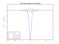
Figure 1: V(x),$\langle x|\psi_{0i}(0)\rangle$

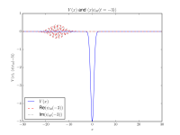
Figure 2: V(x),$\langle x|\psi_{0i}(-3)\rangle$

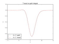
Figure 3: Re(T) exact vs path integral

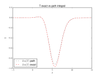
Figure 4: Im(T) exact vs. path integral

This work supported by the U.S. Department of Energy, Office of Science, Grant number: DE-SC0016457.

References

- [1] Feynman, R.: Space-time approach to non-relativistic quantum mechanics, Reviews of Modern Physics,2,367(1948)
- [2] Feynman, R. and Hibbs, A. R.: Quantum Mechanics and Path Integrals, McGraw-Hill, USA (1965)
- [3] Metropolis, N. and Ulam S.: The Monte Carlo method, Journal of the American Statistical Association, 44,335(1949)
- [4] Muldowney, P.: A Modern Theory of Random Variation, Wiley, NJ, (2012)
- [5] Nathanson, Ekaterina S. and Jørgensen, Palle, E.T.: A global solution to the Schrø:dinger equation: From Henstock to Feynman, J. Math. Phys. 56, 092102(2015)
- [6] Nathanson, Ekaterina S.: Path integration with non-positive distributions and applications to the Schrödinger equation, University of Iowa Thesis, (2015)
- [7] Henstock, R.: Theory of Integration, Butterworths, London, (1963)
- [8] Bartle, R. G.: A modern theory of integration, American Mathematical Society, Providence, RI (2001)
- [9] Reed, M. and Simon, B.: Methods of Modern Mathematical Physics, Academic Press, San Diego, p 295(1980)
- [10] Polyzou, W. N. and Nathanson, E. S.: Scattering using real-time path integrals, arxiv:1712.00046,(2018)
- [11] Abramowitz, M. and Stegun, I.: Handbook of Mathematical Functions, National Bureau of Standards, Washington, DC, (1964)