Electron – phonon coupling in Eliashberg – McMillan theory beyond adiabatic approximation

Abstract

Eliashberg – McMillan theory of superconductivity is essentially based on the adiabatic approximation. Small parameter of perturbation theory is given by $\lambda\frac{\Omega_{0}}{E_{F}}\ll 1$, where $\lambda$ is the dimensionless electron – phonon coupling constant, $\Omega_{0}$ is characteristic phonon frequency, while $E_{F}$ is Fermi energy of electrons. Here we present an attempt to describe electron – phonon interaction within Eliashberg – McMillan approach in situation, when characteristic phonon frequency $\Omega_{0}$ becomes large enough (comparable or exceeding the Fermi energy $E_{F}$). We consider the general definition of electron – phonon pairing coupling constant $\lambda$, taking into account the finite value of phonon frequency. Also we obtain the simple expression for the generalized coupling constant $\tilde{\lambda}$, which determines the mass renormalization, with the account of finite width of conduction band, and describing the smooth transition from the adiabatic regime to the region of strong nonadiabaticity. In the case of strong nonadiabaticity, when $\Omega_{0}\gg E_{F}$, the new small parameter appears $\lambda\frac{E_{F}}{\Omega_{0}}\sim\lambda\frac{D}{\Omega_{0}}\ll 1$ ($D$ is conduction band half – width), and corrections to electronic spectrum become irrelevant. At the same time, the temperature of superconducting transition $T_{c}$ in antiadiabatic limit is still determined by Eliashberg – McMillan coupling constant $\lambda$, while the preexponential factor in the expression for $T_{c}$, conserving the form typical of weak – coupling theory, is determined by the bandwidth (Fermi energy). For the case of interaction with a single optical phonon we derive the single expression for $T_{c}$, valid both in adiabatic and antiadiabatic regimes and describing the continuous transition between these two limiting cases. The results obtained are discussed in the context of superconductivity in FeSe/STO.

I Introduction

Eliashberg – McMillan superconductivity theory is the most successful approach to microscopic description of the properties of conventional superconductors with electron – phonon mechanism of Cooper pairing Scal ; Izy ; All . It basic principles can be directly generalized also for the description of non – phonon pairing mechanism in new high – temperature superconductors. Recently this theory was successfully applied to the description of record breaking superconductivity in hydrides at high pressures Grk-Krs .

It is widely known that Eliashberg – Mc Millan theory is essentially based on the applicability of adiabatic approximation and Migdal’s theorem Mig , which allows the neglect of vertex corrections in calculations of electron – phonon coupling in typical metals. In this case the correct small parameter of perturbation theory is $\lambda\frac{\Omega_{0}}{E_{F}}\ll 1$, where $\lambda$ is the dimensionless Eliashberg – McMillan electron – phonon coupling constant, $\Omega_{0}$ is characteristic phonon frequency and $E_{F}$ is Fermi energy of electrons. In particular, this leads to the common opinion, that vertex corrections in this theory can be neglected even for $\lambda>1$, due to the validity of inequality $\frac{\Omega_{0}}{E_{F}}\ll 1$, characteristic for typical metals. This is certainly correct in continuous approximation, when we neglect the effects of lattice discreteness on electron spectrum.

The discreteness of the lattice leads to the breaking of Migdal’s theorem for $\lambda\sim 1$ due to polaronic effects Alx ; Scl . At the same time, for the region of $\lambda<1$ we can safely neglect these effects Scl . In the following we shall consider only the continuous case, limiting our discussion to not so large values of electron – phonon coupling $\lambda$.

Recently a number of superconductors was discovered, where the adiabatic approximation can not be considered valid, and characteristic frequencies of phonons are of the order or even greater than Fermi energy. We bear in mind mainly superconductors based on FeSe monolayers, mostly the systems like single – atomic layer of FeSe on the SrTiO₃ substrate (FeSe/STO) UFN . For these systems this was first noted by Gor’kov Gork_1 ; Gork_2 , while discussing the idea of possible $T_{c}$ enhancement in FeSe/STO due to interaction with high – energy optical phonons in SrTiO₃ UFN .

II Self – energy and electron – phonon coupling constant

Consider the second – order (in electron – phonon coupling) diagram shown in Fig. 1. At first it is sufficient to consider a metal in normal (non superconducting) state. We can perform our analysis either in Matsubara technique ($T\neq 0$) or in $T=0$ technique. In particular, making all calculations in finite temperature technique, after the analytic continuation from Matsubara to real frequencies $i\omega_{n}\to\varepsilon\pm i\delta$ and in the limit of $T=0$, the contribution of diagram Fig. 1 can be written in the standard form Scal ; Schr :

$$\Sigma(\varepsilon,{\bf p})=\sum_{\bf p^{\prime},\alpha}|g^{\alpha}_{\bf pp^{\prime}}|^{2}\Biggl{\{}\frac{f_{\bf p^{\prime}}}{\varepsilon-\varepsilon_{\bf p^{\prime}}+\Omega^{\alpha}_{\bf p-p^{\prime}}-i\delta}$$

$$+\frac{1-f_{\bf p^{\prime}}}{\varepsilon-\varepsilon_{\bf p^{\prime}}-\Omega^{\alpha}_{\bf p-p^{\prime}}+i\delta}\Biggr{\}}$$ (1)

where in notations of Fig. 1 we have ${\bf k=p}$ and ${\bf p^{\prime}=p+q}$. Here $g^{\alpha}_{\bf p,p^{\prime}}$ is Fröhlich electron – phonon coupling constant, $\varepsilon_{\bf p}$ is electronic spectrum with energy zero taken at the Fermi level, $\Omega^{\alpha}_{\bf q}$ is phonon spectrum, $f_{\bf p}$ is the Fermi distribution (step – like).

In particular, for the imaginary part of self – energy at positive frequencies we have:

$$Im\Sigma(\varepsilon>0,{\bf p})=-\pi\sum_{\bf p^{\prime},\alpha}|g^{\alpha}_{\bf pp^{\prime}}|^{2}(1-f_{\bf p^{\prime}})\delta(\varepsilon-\varepsilon_{\bf p^{\prime}}-\Omega^{\alpha}_{\bf p-p^{\prime}})$$ (2)

In these expressions index $\alpha$ enumerates the branches of phonon spectrum. In the following we just drop it for brevity.

Eq. (1) can be identically written as:

$$\Sigma(\varepsilon,{\bf p})=\int d\omega\sum_{\bf p^{\prime}}|g_{\bf pp^{\prime}}|^{2}\delta(\omega-\Omega_{\bf p-p^{\prime}})\times$$

$$\times\Biggl{\{}\frac{f_{\bf p^{\prime}}}{\varepsilon-\varepsilon_{\bf p^{\prime}}+\omega-i\delta}+\frac{1-f_{\bf p^{\prime}}}{\varepsilon-\varepsilon_{\bf p^{\prime}}-\omega+i\delta}\Biggr{\}}$$ (3)

In Eliashberg – McMillan approach we usually get rid of explicit momentum dependence here by averaging the matrix element of electron – phonon interaction over surfaces of constant energies, corresponding to initial and final momenta ${\bf p}$ and ${\bf p^{\prime}}$, which usually reduces to the averaging over corresponding Fermi surfaces, as phonon scattering takes place only within the narrow energy interval close to the Fermi level, with effective width of the order of double Debye frequency $2\Omega_{D}$, and in typical metals we always have $\Omega_{D}\ll E_{F}$. This is achieved by the following replacement:

$$|g_{\bf pp^{\prime}}|^{2}\delta(\omega-\Omega_{\bf p-p^{\prime}})\Longrightarrow$$

$$\frac{1}{N(0)}\sum_{\bf p}\frac{1}{N(0)}\sum_{\bf p^{\prime}}|g_{\bf pp^{\prime}}|^{2}\delta(\omega-\Omega_{\bf p-p^{\prime}})\delta(\varepsilon_{\bf p})\delta(\varepsilon_{\bf p^{\prime}})$$

$$\equiv\frac{1}{N(0)}\alpha^{2}(\omega)F(\omega)$$ (4)

where in the last expression we have introduced the definition of Eliashberg function $\alpha^{2}(\omega)$ and $F(\omega)=\sum_{\bf q}\delta(\omega-\Omega_{\bf q})$ is the phonon density of states.

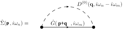
Figure 1: Second – order diagram for self – energy. Dashed line — phonon Green’s function $D^{(0)}$, continuous line — electron Green’s function $G$ in Matsubara representation.

In the case, when phonon energy becomes comparable with or even exceeds the Fermi energy, electron scattering is effective not in the narrow energy layer around the Fermi surface, but in a wider energy interval of the order of $\Omega_{0}\sim E_{F}$, where $\Omega_{0}$ is a characteristic phonon frequency (e.g. of an optical phonon). Then, for the case of initial $|{\bf p}|\sim p_{F}$ the averaging over ${\bf p^{\prime}}$ in expression like (4) should be done over the surface of constant energy, corresponding to $E_{F}+\Omega_{\bf p-p^{\prime}}$, as is shown in Fig. (2). Then the Eq. (4) is directly generalized as:

$$\noindent|g_{\bf pp^{\prime}}|^{2}\delta(\omega-\Omega_{\bf p-p^{\prime}})\Longrightarrow$$

$$\frac{1}{N(0)}\sum_{\bf p}\frac{1}{N(0)}\sum_{\bf p^{\prime}}|g_{\bf pp^{\prime}}|^{2}\times$$

$$\times\delta(\omega-\Omega_{\bf p-p^{\prime}})\delta(\varepsilon_{\bf p})\delta(\varepsilon_{\bf p^{\prime}}-\Omega_{\bf p-p^{\prime}})$$

$$\equiv\frac{1}{N(0)}\alpha^{2}(\omega)F(\omega)$$

(5)

which in the last $\delta$-function simply corresponds to transition from chemical potential $\mu$ to $\mu+\Omega_{\bf p-p^{\prime}}$. We remind that, as usual, the energy zero is taken at $\mu=0$.

After the replacement like (4) or (5) the explicit momentum dependence of the self – energy disappears and in fact in the following we are dealing with Fermi surface average $\Sigma(\varepsilon)\equiv\frac{1}{N(0)}\sum_{\bf p}\delta(\varepsilon_{\bf p})\Sigma({\varepsilon,{\bf p}})$, which is now written as:

$$\Sigma(\varepsilon)=\int d\varepsilon^{\prime}\int d\omega\alpha^{2}(\omega)F(\omega)\Biggl{\{}\frac{f(\varepsilon^{\prime})}{\varepsilon-\varepsilon^{\prime}+\omega-i\delta}$$

$$+\frac{1-f(\varepsilon^{\prime})}{\varepsilon-\varepsilon^{\prime}-\omega+i\delta}\Biggr{\}}$$ (6)

This expression forms the basis of Eliashberg – McMillan theory and determines the structure of Eliashberg equations for the description of superconductivity.

III Mass renormalization and electron – phonon coupling constant

For the case of self – energy dependent only on frequency (and not on momentum) we have the following simple expressions, relating mass renormalization of an electron to the residue a the pole of the Green’s function Diagr :

$$Z^{-1}=1-\left.\frac{\partial\Sigma(\varepsilon)}{\partial\varepsilon}\right|_{\varepsilon=0}$$ (7)

$$m^{\star}=\frac{m}{Z}=m\left.\left(1-\frac{\partial\Sigma(\varepsilon)}{\partial\varepsilon}\right|_{\varepsilon=0}\right)$$ (8)

Then from Eq. (6) by direct calculations (all integrals here are in infinite limits) we obtain:

$$-\left.\frac{\partial\Sigma(\varepsilon)}{\partial\varepsilon}\right|_{\varepsilon=0}=\int d\varepsilon^{\prime}\int d\omega\alpha^{2}(\omega)F(\omega)\Biggl{\{}\frac{f(\varepsilon^{\prime})}{(\omega-\varepsilon^{\prime}-i\delta)^{2}}$$

$$+\frac{1-f(\varepsilon^{\prime})}{(\omega+\varepsilon^{\prime}+i\delta)^{2}}\Biggr{\}}=2\int_{0}^{\infty}\frac{d\omega}{\omega}\alpha^{2}(\omega)F(\omega)$$

(9)

so that introducing the dimensionless Eliashberg – McMillan electron – phonon coupling constant as:

$$\lambda=2\int_{0}^{\infty}\frac{d\omega}{\omega}\alpha^{2}(\omega)F(\omega)$$ (10)

we immediately obtain the standard expression for electron mass renormalization due to electron – phonon interaction:

$$m^{\star}=m(1+\lambda)$$ (11)

The function $\alpha^{2}(\omega)F(\omega)$ in the expression for Eliashberg – McMillan electron – phonon coupling constant (10) should be calculated according to (4) or (5) depending on the relation between Fermi energy $E_{F}$ and characteristic phonon frequency $\Omega$ (roughly estimated by $\Omega_{D}$). As long as $\Omega\ll E_{F}$ we can use the standard expression (4), while in case of $\Omega\sim E_{F}$ we should use (5). In principle all these facts are known for a long time — implicitly these results were mentioned e.g. in Allen’s paper Allen , but misunderstandings still appear Kulich . Using Eq. (5) we can rewrite (10) in the following form:

$$\lambda=\frac{2}{N(0)}\int\frac{d\omega}{\omega}\sum_{\bf p}\sum_{\bf p^{\prime}}|g_{\bf pp^{\prime}}|^{2}\times$$

$$\times\delta(\omega-\Omega_{\bf p-p^{\prime}})\delta(\varepsilon_{\bf p})\delta(\varepsilon_{\bf p^{\prime}}-\Omega_{\bf p-p^{\prime}})$$ (12)

which gives the most general expression to calculate the electron – phonon constant $\lambda$, determining Cooper pairing in Eliashberg – McMillan theory.

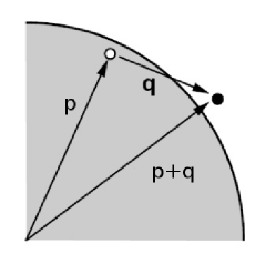
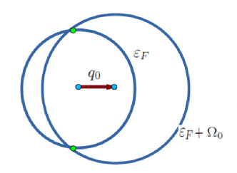
Figure 2: (a) Elementary act of electron – phonon scattering in the vicinity of the Fermi surface. (b) Surfaces of constant energy for initial and final states of an electron scattered by an optical phonon with energy comparable to Fermi energy. Averaging of the matrix element of interaction in (12) or (14) goes over the intersection region of these surfaces.

IV Electron interaction with optical phonons with “forward” scattering

The discovery of high – temperature superconductivity in single – atomic layers of FeSe on SrTiO₃ (FeSe/STO) and similar substrates, with record – breaking, for iron – based superconductors, critical temperature $T_{c}$, nearly an order of magnitude higher than in the bulk FeSe (see review in Ref. UFN ), has sharpened the problem of search of microscopic mechanism of $T_{c}$ enhancement. It was followed by the discovery in ARPES experiments on FeSe/STO of the so called “replicas” of conduction band FeSe_ARPES_Nature , which lead to the idea of $T_{c}$ enhancement due to interaction of conduction electrons with optical phonons of SrTiO₃, with rather high energies (frequencies) $\sim$ 100 meV and “nearly forward” scattering (i.e. with small transferred momentum of the phonon) due to the peculiarities of interaction with optically active Ti – O dipoles at the interface with STO. The model of such scattering introduced in Ref. FeSe_ARPES_Nature has revived the interest to earlier model of $T_{c}$ enhancement, proposed by Dolgov and Kulić, due to “forward” scattering DaDoKuO ; Kulich , which was further developed and applied to FeSe/STO in Refs. Rade_1 ; Rade_2 . In fact, this model explains the formation of the “replicas” of conduction band and the possibility to achieve high values of $T_{c}$, though its basic conclusions were criticized (from different points of view) in Refs. NPS_1 ; NPS_2 ; Saw and are still under discussion.

One of the major circumstances, which was not payed much attention in Refs. FeSe_ARPES_Nature ; Rade_1 ; Rade_2 , was the nonadiabatic character, as noted by Gor’kov Gork_1 ; Gork_2 , of FeSe electrons interaction with optical phonons of STO. The Fermi energy in conduction band of FeSe/STO is small, of the order of 50-60 meV UFN ; FeSe_ARPES_Nature , which by itself is a serious problem for theoretical explanation NPS_1 ; NPS_2 . Correspondingly, the energy of optical phonons $\sim$ 100 meV exceeds is nearly twice, leading to strong enough breaking of adiabaticity. Let us see, first of all, the consequences of this fact for calculations of electron – phonon coupling constant in Eliashberg – McMillan approach.

Consider a particular example of electrons interacting with a single optical (Einstein – like) phonon mode with high – enough frequency $\Omega_{0}$, which scatters essentially “forward”. The general qualitative picture of such scattering is shown in Fig. 2. In this case in Eq. (12) the density of phonon states is simply $F(\omega)=\delta(\omega-\Omega_{0})$, and for the momentum dependence of interaction with optical phonon at FeSe/STO interface we can assume the characteristic dependence, obtained in Ref. FeSe_ARPES_Nature :

$$g({\bf q})=g_{0}\exp(-|{\bf q}|/q_{0}),$$ (13)

where the typical value of $q_{0}\sim 0.1\frac{\pi}{a}\ll p_{F}$ (where $a$ is the lattice constant and $p_{F}$ is the Fermi momentum), leading to nearly “forward” scattering of electrons by optical phonons.

Then the dimensionless pairing constant of electron – phonon interaction in Eliashberg theory is written as:

$$\lambda=\frac{2}{N(0)\Omega_{0}}\sum_{\bf p}\sum_{\bf q}|g_{\bf q}|^{2}\delta(\varepsilon_{\bf p})\delta(\varepsilon_{\bf p+q}-\Omega_{0})$$ (14)

As in FeSe/STO we have in fact $\Omega_{0}>E_{F}$ the finite value in the second $\delta$-function here should be taken into account.

For simple estimates let us assume the linearized form of electronic spectrum ($v_{F}$ is Fermi velocity): $\varepsilon_{\bf p}\approx v_{F}(|{\bf p}|-p_{F})$, which allows to perform all calculations analytically. Then, substituting (13) into (14) and considering two – dimensional case, after calculating all integrals here we obtain NPS_2 :

$$\lambda=\frac{g_{0}^{2}a^{2}}{\pi^{2}v_{F}^{2}}K_{1}\left(\frac{2\Omega_{0}}{v_{F}q_{0}}\right),$$ (15)

where $K_{1}(x)$ is Bessel function of imaginary argument (McDonald function). Using the well – known asymptotic form of $K_{1}(x)$ and dropping a number of irrelevant constants, we have:

$$\lambda\sim\lambda_{0}\frac{q_{0}}{4\pi p_{F}},$$ (16)

for $\frac{\Omega_{0}}{v_{F}q_{0}}\ll 1$, and

$$\lambda\sim\lambda_{0}\frac{\Omega_{0}}{\pi E_{F}}\sqrt{\frac{v_{F}q_{0}}{\Omega_{0}}}\exp\left(-\frac{2\Omega_{0}}{v_{F}q_{0}}\right),$$ (17)

for $\frac{\Omega_{0}}{v_{F}q_{0}}\gg 1$.

Here we introduced the standard dimensionless electron – phonon coupling constant:

$$\lambda_{0}=\frac{2g_{0}^{2}}{\Omega_{0}}N(0),$$ (18)

where $N(0)$ is the density of electronic states at the Fermi level per single spin projection.

The result (16) is known Rade_1 ; Rade_2 and by itself is rather unfavorable for significant $T_{c}$ enhancement in model under discussion. Even worse is the situation if we take into account the large values of $\Omega_{0}$, as pairing constant becomes exponentially suppressed for $\frac{\Omega_{0}}{v_{F}q_{0}}>1$, which is typical for FeSe/STO interface, where $\Omega_{0}>E_{F}\gg v_{F}q_{0}$ UFN . This makes the enhancement of $T_{c}$ due to interaction of FeSe electrons with optical phonons of STO rather improbable. In fact, similar conclusions were made from first – principles calculations in Ref. Johnson , where the dependence of Eliashberg coupling constant on frequency of the optical phonon in STO was also taken into account. However, the effect of suppression of this constant was much smaller, which was probably due to unrealistically large values of the Fermi energy, obtained form LDA calculations of electronic spectrum of FeSe/STO, which does not account for the role of correlations Johnson . Correspondingly, in Ref. Johnson they always had $\Omega_{0}\ll E_{F}$. The account of correlations within LDA+DMFT calculations, performed in Refs. NPS_1 ; NPS_2 , allowed to obtain the values of Fermi energy in conduction band of FeSe/STO in accordance with ARPES data, which show that in this system we meet with antiadiabatic situation with $\Omega_{0}>E_{F}$.

Certainly, the results obtained above in the asymptotic of high frequencies $\Omega_{0}$ depend on the form of momentum dependence in Eq. (13). For example, if we choose the Gaussian form of interaction fall with transferred momentum, we shall obtain more fast Gaussian suppression with frequency in the limit of Eq. (17). In general case, for fast enough fall of interaction in (13) on the scale of $q_{0}$ we shall always obtain rather fast suppression of coupling constant for $\Omega_{0}\gg v_{F}q_{0}$.

For a more realistic case, when the optical phonon scatters electrons not only in “forward” direction, but in a wide interval of transferred momenta (as it follows e.g. from first – principles calculations of Ref. Johnson ), in the above expression we have simply to use large enough value of the parameter $q_{0}$. Choosing e.g. $q_{0}\sim 4\pi p_{F}$ and using the low frequency limit (16) we immediately obtain $\lambda\approx\lambda_{0}$, i.e. the standard result. Similarly, parameter $q_{0}$ can be taken equal to an inverse lattice vector $2\pi/a$. Then for $q_{0}\sim 2\pi/a$ from (16) we obtain:

$$\lambda\sim\lambda_{0}\frac{1}{2p_{F}a}\sim\lambda_{0}$$ (19)

for typical $p_{F}\sim 1/2a$. In general case there always remain the dependence on the value of Fermi momentum and cutoff parameter (cf. similar analysis in Ref. Diagr ).

In the limit of (17), assuming $q_{0}\sim p_{F}$ we immediately obtain:

$$\lambda\sim\frac{\sqrt{2}}{\pi}\lambda_{0}\sqrt{\frac{\Omega_{0}}{E_{F}}}\exp\left(-\frac{\Omega_{0}}{E_{F}}\right),$$ (20)

which simply signifies the effective interaction cutoff for $\Omega_{0}>E_{F}$ in antiadiabatic limit. This fact was stressed by Gor’kov in Refs. Gork_1 ; Gork_2 .

V Effects of finite bandwidth and antiadiabatic limit

As was already noted above, the usual Migdal – Eliashberg approach is totally justified in adiabatic approximation, related for usual electron – phonon systems (metals) with the presence of a small parameter $\Omega_{D}/E_{F}\ll 1$ (or $\Omega_{0}/E_{F}\ll 1$ for the case of a single optical phonon with frequency $\Omega_{0}$). The true parameter of perturbation theory in this case is given by $\lambda(\Omega_{0}/E_{F})$, which is small even for $\lambda\sim 1$. The presence of this small parameter allows us to limit ourselves to calculations of a simple diagram of the second order over electron – phonon interaction considered above, and neglect all vertex corrections (Migdal’s theorem) Mig . These conditions are broken in FeSe/STO system, where $\Omega_{0}\sim 2E_{F}$.

Our discussion up to now implicitly assumed the conduction band of an infinite width. It is clear that in case of large enough characteristic phonon frequency it may be comparable not only with Fermi energy, but also with conduction band width. Below we shall show that in the limit of strong nonadiabaticity, when $\Omega_{0}\gg E_{F}\sim D$ (where $D$ is the conduction band half-width), in fact, we are dealing with the situation, when a new small parameter of perturbation theory $\lambda D/\Omega_{0}\sim\lambda E_{F}/\Omega_{0}$ appears in the theory.

Let us consider the case of conduction band of the finite width $2D$ with constant density of states (which formally corresponds formally to two – dimensional case). The Fermi level as above is considered as an origin of energy scale and we assume the typical case of half – filled band. Then (6) reduces to:

$$\noindent\Sigma(\varepsilon)=\int_{-D}^{D}d\varepsilon^{\prime}\int d\omega\alpha^{2}(\omega)F(\omega)\Biggl{\{}\frac{f(\varepsilon^{\prime})}{\varepsilon-\varepsilon^{\prime}+\omega-i\delta}$$

$$+\frac{1-f(\varepsilon^{\prime})}{\varepsilon-\varepsilon^{\prime}-\omega+i\delta}\Biggr{\}}=$$

$$\noindent=\int_{0}^{D}d\varepsilon^{\prime}\int d\omega\alpha^{2}(\omega)F(\omega)\Biggl{\{}\frac{1}{\varepsilon+\varepsilon^{\prime}+\omega-i\delta}$$

$$+\frac{1}{\varepsilon-\varepsilon^{\prime}-\omega+i\delta}\Biggr{\}}=$$

$$=\int d\omega\alpha^{2}(\omega)F(\omega)\Biggl{\{}\ln\frac{\varepsilon+D+\omega-i\delta}{\varepsilon-D-\omega+i\delta}$$

$$\noindent-\ln\frac{\varepsilon+\omega-i\delta}{\varepsilon-\omega+i\delta}\Biggr{\}}$$

For the model of a single optical phonon $F(\omega)=\delta(\omega-\Omega_{0})$ and we immediately obtain:

$$\Sigma(\varepsilon)=\alpha^{2}(\Omega_{0})F(\Omega_{0})\Biggl{\{}\ln\frac{\varepsilon+D+\Omega_{0}-i\delta}{\varepsilon-D-\Omega_{0}+i\delta}$$

$$\noindent-\ln\frac{\varepsilon+\Omega_{0}-i\delta}{\varepsilon-\Omega_{0}+i\delta}\biggr{\}}=$$

$$=\alpha^{2}(\Omega_{0})F(\Omega_{0})\ln\Biggl{\{}\frac{\varepsilon+D+\Omega_{0}-i\delta}{\varepsilon-D-\Omega_{0}+i\delta}\frac{\varepsilon-\Omega_{0}+i\delta}{\varepsilon+\Omega_{0}-i\delta}\Biggr{\}}$$ (22)

Correspondingly, form (V) we get:

$$-\left.\frac{\partial\Sigma(\varepsilon)}{\partial\varepsilon}\right|_{\varepsilon=0}=2\int_{0}^{D}d\varepsilon^{\prime}\int_{0}^{\infty}d\omega\alpha^{2}(\omega)F(\omega)\frac{1}{(\omega+\varepsilon^{\prime})^{2}}$$

$$\noindent=2\int_{0}^{\infty}d\omega\alpha^{2}(\omega)F(\omega)\frac{D}{\omega(\omega+D)}$$

(23)

and we can define the the generalized coupling constant as:

$$\tilde{\lambda}=2\int_{0}^{\infty}\frac{d\omega}{\omega}\alpha^{2}(\omega)F(\omega)\frac{D}{\omega+D}$$ (24)

which for $D\to\infty$ reduces to the usual Eliashberg – McMillan constant (10), while for $D\to 0$ is gives the “antiadiabatic” coupling constant:

$$\lambda_{D}=2D\int\frac{d\omega}{\omega^{2}}\alpha^{2}(\omega)F(\omega)$$ (25)

Eq. (24) describes the smooth transition between the limits of wide and narrow conduction bands. Mass renormalization in general case is determined by $\tilde{\lambda}$:

$$m^{\star}=m(1+\tilde{\lambda})$$ (26)

In strong antiadiabatic limit of $D\ll\Omega_{0}$, after elementary calculations we obtain from (V):

$$Re\Sigma(\varepsilon)=2D\int d\omega\alpha^{2}(\omega)F(\omega)\frac{\varepsilon}{\varepsilon^{2}-\omega^{2}}$$ (27)

and from (22)

$$Re\Sigma(\varepsilon)=\alpha^{2}(\Omega_{0})\frac{2D\varepsilon}{\varepsilon^{2}-\Omega^{2}_{0}}=\lambda_{D}\frac{\Omega^{2}_{0}\varepsilon}{\varepsilon^{2}-\Omega^{2}_{0}}$$ (28)

For the model of a single optical phonon with frequency $\Omega_{0}$ we have:

$$\tilde{\lambda}=\frac{2}{\Omega_{0}}\alpha^{2}(\Omega_{0})\frac{D}{\Omega_{0}+D}=\lambda\frac{D}{\Omega_{0}+D}=\lambda_{D}\frac{\Omega_{0}}{\Omega_{0}+D}$$ (29)

where Eliashberg – McMillan constant is:

$$\lambda=2\int_{0}^{\infty}\frac{d\omega}{\omega}\alpha^{2}(\omega)F(\omega)=\alpha^{2}(\Omega_{0})\frac{2}{\Omega_{0}}$$ (30)

and $\lambda_{D}$ reduces to:

$$\lambda_{D}=2\alpha^{2}(\Omega_{0})\frac{D}{\Omega_{0}^{2}}=2\alpha^{2}(\Omega_{0})\frac{1}{\Omega_{0}}\frac{D}{\Omega_{0}}$$ (31)

where in the last expression we have introduced the new small parameter $D/\Omega_{0}\ll 1$, appearing in strong antiadiabatic limit. Correspondingly, in this limit we always have:

$$\lambda_{D}=\lambda\frac{D}{\Omega_{0}}\sim\lambda\frac{E_{F}}{\Omega_{0}}\ll\lambda$$ (32)

so that for reasonable values of $\lambda$ (even up to a strong coupling region of $\lambda\sim 1$) “antiadiabatic” coupling constant remains small. Obviously, all vertex corrections are also small in this limit, as was shown by direct calculations in Ref. Ikeda , which went rather unnoticed. Thus we come to an unexpected conclusion — in the limit of strong nonadiabaticity the electron – phonon coupling becomes weak!

For imaginary part of self – energy in strong antiadiabatic limit we easily obtain:

$$Im\Sigma(\varepsilon>0)=-i2\pi D\varepsilon\int d\omega\alpha^{2}(\omega)F(\omega)\delta(\varepsilon^{2}-\omega^{2})=$$

$$-i2\pi D\varepsilon\int d\omega\alpha^{2}(\omega)F(\omega)\frac{1}{2\varepsilon}\{\delta(\varepsilon-\omega)+\delta(\varepsilon+\omega)\}-$$

$$=-i\pi D\alpha^{2}(\varepsilon)F(\varepsilon)$$

(33)

which in a single phonon model reduces to:

$$Im\Sigma(\varepsilon>0)=-i\pi D\alpha^{2}(\Omega_{0})\delta(\varepsilon-\Omega_{0})=$$

$$=-\frac{i\pi}{2}\lambda_{D}\Omega^{2}_{0}\delta(\varepsilon-\Omega_{0})$$ (34)

From these expressions it is clear that this imaginary part is not particularly important in this limit (being non zero only for $\varepsilon=\Omega_{0}$), and equation for the real part of electronic dispersion:

$$\varepsilon-\varepsilon_{\bf p}-Re\Sigma(\varepsilon)=0$$ (35)

is now:

$$\varepsilon-\varepsilon_{\bf p}-\alpha^{2}(\Omega_{0})\frac{2D\varepsilon}{\varepsilon^{2}-\Omega^{2}_{0}}=0$$ (36)

Correspondingly, for $\varepsilon\sim\varepsilon_{\bf p}$ we can write:

$$\varepsilon-\varepsilon_{\bf p}-\alpha^{2}(\Omega_{0})\frac{2D\varepsilon_{\bf p}}{\varepsilon_{\bf p}^{2}-\Omega^{2}_{0}}=0$$ (37)

which for $\varepsilon_{\bf p}\to 0$ gives a small correction to the spectrum:

$$\varepsilon\approx\varepsilon_{\bf p}-\alpha^{2}(\Omega_{0})\frac{2D}{\Omega^{2}_{0}}\varepsilon_{\bf p}=\varepsilon_{\bf p}-\lambda_{D}\varepsilon_{\bf p}=\varepsilon_{\bf p}(1-\lambda_{D})$$ (38)

obviously reducing to a small ($\lambda_{D}\ll 1$) renormalization of the effective mass (26).

Physically, the weakness of electron – phonon coupling in strong nonadiabatic limit is pretty clear — when ions move much faster than electrons, these have no time to “fit” the rapidly changing configuration of ions and, in these sense, only weakly react on their movement.

VI Eliashberg equations and the temperature of superconducting transition

All analysis above was performed for the normal state of a metal. The problem arises, to which extent the results obtained can be generalized for the case of a metal in superconducting state? In particular, what coupling constant ($\lambda$, $\tilde{\lambda}$ or $\lambda_{D}$) determines the temperature of superconducting transition $T_{c}$ an antiadiabatic limit? Let us analyze the situation within appropriate generalization of Eliashberg equations.

Taking into account that in antiadiabatic approximation vertex corrections are irrelevant and neglecting the direct Coulomb interaction, Eliashberg equations can be derived by calculating the diagram of Fig. 1, where electronic Green’s function in superconducting state is taken in Nambu’s matrix representation. For real frequencies this is written in the following standard form Izy :

$$G(\varepsilon,{\bf p})=\frac{Z(\varepsilon)\varepsilon\tau_{0}+\varepsilon_{\bf p}\tau_{3}+Z(\varepsilon)\Delta(\varepsilon)\tau_{1}}{Z^{2}(\varepsilon)\varepsilon^{2}-Z^{2}(\varepsilon)\Delta^{2}(\varepsilon)-\varepsilon^{2}_{\bf p}}$$ (39)

which corresponds to the matrix of self – energy:

$$\Sigma(\varepsilon,{\bf p})=[1-Z(\varepsilon)]\varepsilon\tau_{0}+Z(\varepsilon)\Delta(\varepsilon)\tau_{1}$$ (40)

where $\tau_{i}$ are standard Pauli matrices, while functions of mass renormalization $Z(\varepsilon)$ and energy gap $\Delta(\varepsilon)$ are determined from solution of integral Eliashberg equations, which in representation of real frequencies are written as Izy :

$$[1-Z(\varepsilon)]\varepsilon=-\int_{-D}^{D}d\varepsilon^{\prime}K(\varepsilon^{\prime},\varepsilon)Re\frac{\varepsilon^{\prime}}{\sqrt{\varepsilon^{\prime 2}-\Delta^{2}({\varepsilon^{\prime}})}}sign\,\varepsilon$$ (41)

$$Z(\varepsilon)\Delta(\varepsilon)=\int_{-D}^{D}K(\varepsilon^{\prime},\varepsilon)Re\frac{\Delta(\varepsilon^{\prime})}{\sqrt{\varepsilon^{\prime 2}-\Delta^{2}(\varepsilon^{\prime})}}sign\,\varepsilon$$ (42)

where integral equation kernel has the following form:

$$K(\varepsilon^{\prime},\varepsilon)=\frac{1}{2}\int_{0}^{\infty}d\omega\alpha^{2}(\omega)F(\omega)\times$$

$$\times\Biggl{\{}\frac{th\frac{\varepsilon^{\prime}}{2T}+cth\frac{\omega}{2T}}{\varepsilon^{\prime}+\omega-\varepsilon-i\delta}-\frac{th\frac{\varepsilon^{\prime}}{2T}-cth\frac{\omega}{2T}}{\varepsilon^{\prime}-\omega-\varepsilon-i\delta}\Biggr{\}}$$ (43)

The only difference here from the similar equations of Ref. Izy is the appearance of the finite integration limits, determined by the bandwidth, as well as the absence of the contribution of direct Coulomb repulsion, which will not be discussed here. In fact, Eqs. (41) and (42) are the direct analog of Eqs. (6) and (V) for normal metal and replace them after the transition into superconducting phase.

To determine the temperature of superconducting transition it is sufficient, as usual, to analyze the linearized Eliashberg equations, which are written as:

$$[1-Z(\varepsilon)]\varepsilon=\int_{0}^{D}d\varepsilon^{\prime}\int_{0}^{\infty}d\omega\alpha^{2}(\omega)F(\omega)f(-\varepsilon^{\prime})\times$$

$$\times\left(\frac{1}{\varepsilon^{\prime}+\varepsilon+\omega+i\delta}-\frac{1}{\varepsilon^{\prime}-\varepsilon+\omega-i\delta}\right)$$ (44)

$$Z(\varepsilon)\Delta(\varepsilon)=\int_{0}^{D}\frac{d\varepsilon^{\prime}}{\varepsilon^{\prime}}th\frac{\varepsilon}{2T_{c}}Re\Delta(\varepsilon^{\prime})\times$$

$$\times\int_{0}^{\infty}d\omega\alpha^{2}(\omega)F(\omega)\times$$

$$\times\left(\frac{1}{\varepsilon^{\prime}+\varepsilon+\omega+i\delta}+\frac{1}{\varepsilon^{\prime}-\varepsilon+\omega-i\delta}\right)$$ (45)

For us it is sufficient to consider in these equations the limit of $\varepsilon\to 0$ and look for the solutions $Z(0)=Z$ and $\Delta(0)=\Delta$. Then from (44) we obtain:

$$[1-Z]\varepsilon=-2\varepsilon\int_{0}^{\infty}d\omega\alpha^{2}(\omega)F(\omega)\times$$

$$\times\int_{0}^{D}\frac{d\varepsilon^{\prime}}{(\varepsilon^{\prime}+\omega)^{2}}=$$

$$=-2\varepsilon\int_{0}^{\infty}d\omega\alpha^{2}(\omega)F(\omega)\frac{D}{\omega(\omega+D)}$$

(46)

or

$$Z=1+\tilde{\lambda}$$ (47)

where the constant $\tilde{\lambda}$ was defined above in Eq. (24). Thus, precisely this effective constant determines mass renormalization both in normal and superconducting phases. As was shown above, in the limit of strong antiadiabaticity this renormalization is very small and determined by the limiting value of $\lambda_{D}$ (31).

Situation is different in Eq. (45). In the limit of $\varepsilon\to 0$, using (47) we immediately obtain from (45) the following equation for $T_{c}$

$$1+\tilde{\lambda}=2\int_{0}^{\infty}d\omega\alpha^{2}(\omega)F(\omega)\int_{0}^{D}\frac{d\varepsilon^{\prime}}{\varepsilon^{\prime}(\varepsilon^{\prime}+\omega)}th\frac{\varepsilon^{\prime}}{2T_{c}}$$ (48)

In antiadiabatic limit, when characteristic frequencies of phonons exceed the width of the conduction band, we can neglect $\varepsilon^{\prime}$ as compared to $\omega$ in the denominator of the integrand in (48), so that the equation for $T_{c}$ is rewritten as:

$$1+\tilde{\lambda}\approx 2\int_{0}^{\infty}d\omega\frac{\alpha^{2}(\omega)F(\omega)}{\omega}\int_{0}^{D}\frac{d\varepsilon^{\prime}}{\varepsilon^{\prime}}th\frac{\varepsilon^{\prime}}{2T_{c}}=$$

$$=\lambda\int_{0}^{D}\frac{d\varepsilon^{\prime}}{\varepsilon^{\prime}}th\frac{\varepsilon^{\prime}}{2T_{c}}$$ (49)

where $\lambda$ is Eliashberg – McMillan coupling constant as defined above in Eq. (10). From here we immediately obtain the BCS – type result:

$$T_{c}\sim D\exp\left(-\frac{1+\tilde{\lambda}}{\lambda}\right)$$ (50)

We have seen above, that in antiadiabatic limit we always have $\tilde{\lambda}\to\lambda_{D}\ll\lambda$, so that in the exponent in (50) we can neglect it, so that the expression for $T_{c}$ is reduced simply to to BCS weak coupling formula, with preexponential factor determined by the half – width of the band (Fermi energy), while the pairing coupling constant in the exponential is determined the the general Eliashberg – McMillan expression (taking account the discussion above).

In the model with single optical phonon of frequency $\Omega_{0}$ Eq. (49) has the form:

$$1+\tilde{\lambda}=2\alpha^{2}(\Omega_{0})\int_{0}^{D}\frac{d\varepsilon^{\prime}}{\varepsilon^{\prime}(\varepsilon^{\prime}+\Omega_{0})}th\frac{\varepsilon^{\prime}}{2T_{c}}$$ (51)

Eq. (51) is easily solved (the intgeral here can be taken, as usual, by partial integration) and we obtain:

$$T_{c}\sim D\exp\left(-\frac{1+\tilde{\lambda}+\lambda\ln(\frac{D}{\Omega_{0}}+1)}{\lambda}\right)=$$

$$=\frac{D}{1+\frac{D}{\Omega_{0}}}\exp\left(-\frac{1+\tilde{\lambda}}{\lambda}\right)$$ (52)

where for $\lambda$ is naturally defined by Eq. (30). We see, that in antiadiabatic regime, for $\frac{D}{\Omega_{0}}\ll 1$ this expression reduces to (50), while in adiabatic limit $\frac{D}{\Omega_{0}}\gg 1$ we obtain the usual expression for $T_{c}$ of Eliashberg theory for the case of intermediate coupling:

$$T_{c}\sim\Omega_{0}\exp\left(-\frac{1+\lambda}{\lambda}\right)$$ (53)

Thus, Eq. (51) gives the unified expression for $T_{c}$, which is valid both in adiabatic and antiadiabatic limits, smoothly interpolating between these two limits.

Finally, we come to rather unexpected conclusions — in the limit of strong nonadiabaticity $T_{c}$ is determined by an expression like BCS weak coupling theory, with preexponential determined not by a characteristic phonon frequency, but by Fermi energy (the same conclusion was reached in a recent paper by Gor’kov Gork_2 ), while the pairing coupling constant conserves the standard form of Eliashberg – McMillan theory. The effective coupling constant $\tilde{\lambda}$, tending in antiadiabatic limit to $\lambda_{D}$, determines the mass renormalization, but not the temperature of superconducting transition.

VII Conclusion

In this work we have considered the electron – phonon coupling in Eliashberg – McMillan theory outside the limits of the standard adiabatic approximation. We have obtained some simple expressions for interaction parameters of electrons and phonons in the situation, when the characteristic frequency of phonons $\Omega_{0}$ becomes large enough (comparable or even exceeding the Fermi energy $E_{F}$). In particular, we have analyzed the general definition of the pairing constant $\lambda$, taking into account the finite value of phonon frequency. It was shown, that in a popular model with dominating “forward” scattering it leads to to exponential suppression of the coupling constant for the frequencies $\Omega_{0}\gg v_{F}q_{0}$, where $q_{0}$ defines the characteristic size of the region of transferred momenta, where electrons interact with phonons. Similar situation appears also in the usual case, when $q_{0}$ is of the order of inverse lattice vector, and phonon frequency exceeds the Fermi energy $E_{F}$.

We have obtained a simple expression for electron – phonon coupling constant, $\tilde{\lambda}$, determining the mass renormalization in Eliashberg – McMillan theory, taking into account the finite width of conduction band, which describes the smooth transition from adiabatic regime to the region of strong nonadiabaticity. It was shown, that under the conditions of strong nonadiabaticity, when $\Omega_{0}\gg E_{F}$, a new small parameter $\lambda\frac{E_{F}}{\Omega_{0}}\sim\lambda\frac{D}{\Omega_{0}}\ll 1$ ($D$ is the half – width of conduction band) appears in the theory, and corrections to electron spectrum become, in fact, irrelevant, as well as all vertex corrections. In fact, this allows us to apply the general Eliashberg equations outside the limits of adiabatic approximation in strong antiadiabatic limit. Our results show, that outside the limits of adiabatic approximation, in the limit of strong nonadiabaticity, for superconductivity we have a weak coupling regime. Mass renormalization is small and determined by effective coupling constant $\lambda_{D}$, while the strength of the pairing interaction is determined by the standard Eliashberg – McMillan coupling constant $\lambda\gg\lambda_{D}$, appropriately generalized with the account of finiteness of phonon frequency (comparable or exceeding the Fermi energy). The cutoff of pairing interaction in Cooper channel in antiadiabatic limit, as we have seen above (cf. also Gor’kov’s paper Gork_2 ), takes place at the energies $\sim E_{F}$, in weak approximation (supported by our estimates) possible vertex corrections are irrelevant and for $T_{c}$ we can use the usual expression of BCS theory (50), which was also stressed in Ref. Gork_2 . The small value of $E_{F}$ in FeSe/STO system leads to the conclusion, that the only interaction with antiadiabatic phonons of STO is insufficient to explain the experimentally observed values of $T_{c}$, as far as we limit ourselves to weak coupling approximation ant the value of $\lambda$ dies not exceed 0.25. In this case it is necessary to take into account two pairing mechanisms, those responsible for the formation of initial $T_{c0}$ in the bulk FeSe (phonons or spin fluctuations in FeSe) and those enhancing the pairing due interaction with optical phonons of STO. Appropriate estimates of $T_{c}$, performed in Ref. UFN ; Gork_2 are in reasonable agreement with experiments on FeSe/STO, with no use of the ideas on pairing mechanisms with “forward” scattering. At the same time, our analysis show, that the expression for $T_{c}$ like Eq. (50), which formally has the form of weak coupling approximation of BCS theory, in reality “works” (in the limit of strong nonadiabaticity) also for large enough values of $\lambda$, at least up to $\lambda\sim 1$, when polaronic effects become relevant. Correspondingly, to explain the experimentally observed values of $T_{c}$ in FeSe/STO it may be sufficient to deal only with electron interactions with optical phonons of STO, as far as the values of $\lambda\sim 0.5$ can be realized in this system. However, the realization of such large values of coupling constant here seems rather doubtful in the light of our discussion above (cf. also the results of first – principles calculations of $\lambda$ in Ref. Johnson ).

The separate question, which remained outside our discussion, is the account of direst Coulomb repulsion. In standard Eliashberg – McMillan theory, in adiabatic approximation, when the frequency of phonons is orders of magnitude smaller, than Fermi energy, this repulsion enters via Coulomb pseudopotential $\mu^{\star}$, which is significantly suppressed by Tolmachev logarithm Izy . In antiadiabatic situation this mechanism of suppression does not operate, which creates additional difficulties for realization of superconductivity. In general, the problem of the possible role of Coulomb repulsion in antiadiabatic regime of electron – phonon coupling deserves serious further studies.

This work was partially supported by RFBR grant No. 17-02-00015 and the Program of Fundamental Research of the Presidium of the Russian Academy of Sciences No. 12 “Fundamental problems of high – temperature superconductivity”.

References

- (1) D.J. Scalapino. In “Superconductivity”, p. 449, Ed. by R.D. Parks, Marcel Dekker, NY, 1969
- (2) S.V. Vonsovsky, Yu.A. Izyumov, E.Z. Kurmaev. Sverkhprovodimost’ perekhodnihh metallov ikh splavov i soedinenii. “Nauka”, Moscow, 1977 [Superconductivity of Transition metals, Their Alloys and Compounds, Springer, Berlin – Heidelberg, 1982]
- (3) P.B. Allen, B. Mitrović. Solid State Physics, Vol. Vol. 37 (Eds. F. Seitz, D. Turnbull, H. Ehrenreich), Academic Press, NY, 1982, p. 1
- (4) L.P. Gor’kov, V.Z. Kresin. Rev. Mod. Phys. 90, 011001 (2018)
- (5) A.B. Migdal. Zh. Eksp. Teor. Fiz. 34, 1438 (1958) [Sov. Phys. JETP 7, 996 (1958)]
- (6) A.S. Alexandrov. A.B. Krebs. Usp. Fiz. Nauk 162, 1 (1992) [Physics Uspekhi 35, 345 (1992)]
- (7) I. Esterlis, B. Nosarzewski, E.W. Huang, D. Moritz, T.P. Devereux, D.J. Scalapino, S.A. Kivelson. Phys. Rev. B 97, 140501(R) (2018)
- (8) M.V. Sadovskii. Usp. Fiz. Nauk 178, 1243 (2008) [Physics Uspekhi 51, 1243 (2008)]
- (9) L.P. Gor’kov. Phys. Rev. B93, 054517 (2016)
- (10) L.P. Gor’kov. Phys. Rev. B93, 060507 (2016)
- (11) J.R. Schrieffer. Teorija sverkprovodimosti. Fizmatlit, Moscow, 1968 [Theory of Superconductivity, WA Benjamin, NY, 1964]
- (12) M.V. Sadovskii. Diagrammatika. ICS, Moscow-Izhevsk, 2010 [Diagrammatics, World Scientific, Singapore, 2006]
- (13) P.B. Allen. Phys. Rev. B 6, 2577 (1972)
- (14) M. Kulić. ArXiv:1712.06222
- (15) J.J. Lee, F.T. Schmitt, R.G. Moore, S. Johnston, Y.T. Cui,W. Li, Z.K. Liu, M. Hashimoto, Y. Zhang, D.H. Lu, T.P. Devereaux, D.H. Lee, Z.X. Shen. Nature 515, 245 (2014)
- (16) O.V. Danylenko, O.V. Dolgov, M.L. Kulić, V. Oudovenko. Eur. J. Phys. B 9 201 (1999)
- (17) M.L. Kulić, AIP Conference Proceedings 715 75 (2004)
- (18) L. Rademaker, Y. Wang, T. Berlijn, S. Johnston. New J. Phys. 18 022001 (2016)
- (19) Y. Wang, K. Nakatsukasa, L. Rademaker, T. Berlijn, S. Johnston. Supercond. Sci. Technol. 29, 054009 (2016)
- (20) I.A. Nekrasov, N.S. Pavlov, V.V. Sadovskii. Pis’ma Zh. Eksp. Teor. Fiz. 105, 354 (2017) [JETP Letters 105, 370 (2017)]
- (21) I.A. Nekrasov, N.S. Pavlov, M.V. Sadovskii. Zh. Eksp. Teor. Fiz. 153, 590 (2018) [JETP 126, 485 (2018)]
- (22) Fengmiao Li, G.A. Sawatzky. Phys. Rev. Lett. 120, 237001 (2018)
- (23) Y. Wang, A. Linscheid, T. Berlijn, S. Johnson. Phys. Rev. B 93, 134513 (2016)
- (24) M.A. Ikeda, A. Ogasawara, M.Sugihara. Phys. Lett. A 170, 319 (1992)