Scalable Monte Carlo inference for state-space models

Abstract

We present an original simulation-based method to estimate likelihood ratios efficiently for general state-space models. Our method relies on a novel use of the conditional Sequential Monte Carlo (cSMC) algorithm introduced in Andrieu et al. (2010) and presents several practical advantages over standard approaches. The ratio is estimated using a unique source of randomness instead of estimating separately the two likelihood terms involved. Beyond the benefits in terms of variance reduction one may expect in general from this type of approach, an important point here is that the variance of this estimator decreases as the distance between the likelihood parameters decreases. We show how this can be exploited in the context of Monte Carlo Markov chain (MCMC) algorithms, leading to the development of a new class of exact-approximate MCMC methods to perform Bayesian static parameter inference in state-space models. We show through simulations that, in contrast to the Particle Marginal Metropolis–Hastings (PMMH) algorithm of Andrieu et al. (2010), the computational effort required by this novel MCMC scheme scales very favourably for large data sets.

Keywords: Annealed importance sampling, Particle Markov chain Monte Carlo, Sequential Monte Carlo, State-space models.

^∗Faculty of Engineering and Natural Sciences, Sabancı University, Turkey.

$\dagger$School of Mathematics, Bristol University, UK.

$\ddagger$Department of Statistics, Oxford University, UK.

1 Introduction

State-space models (SMMs) form an important class of statistical model used in many fields; see Douc et al. (2014) for a recent overview. In its simplest form a SSM is comprised of an $(\mathsf{X},\mathcal{X})$-valued latent Markov chain $\{X_{t};t\geq 1\},$ and a $(\mathsf{Y},\mathcal{Y})$-valued observed process $\{Y_{t};t\geq 1\}$. The latent process has initial probability with density $\eta_{\theta}(x_{1})$ and transition density $f_{\theta}(x_{t-1},x_{t})$; both probability densities defined on $\mathsf{X}$ and with respect to a common dominating measure on $(\mathsf{X},\mathcal{X})$ denoted generically as ${\rm d}x$ and parametrized by some $\theta\in\Theta\subset\mathbb{R}^{d_{\theta}}$. Naturally, non-dynamical models for which $f_{\theta}(x_{t-1},x_{t})=f_{\theta}(x_{t})$ form a particular case. The observation at time $t$ is assumed conditionally independent of all other random variables given $X_{t}=x_{t}$ and its conditional observation density is $g_{\theta}(x_{t},y_{t})$ on $\mathsf{Y}$ with respect to the dominating measure ${\rm d}y$ on $(\mathsf{Y},\mathcal{Y})$. For a given value $\theta\in\Theta$ we will refer to this model as $\mathscr{M}_{\theta}$, and the corresponding joint density of the latent and observed variables up to time $T$ is

$$p_{\theta}(x_{1:T},y_{1:T})=\mu_{\theta}(x_{1})\prod_{t=2}^{T}f_{\theta}(x_{t-1},x_{t})\prod_{t=1}^{T}g_{\theta}(x_{t},y_{t})\;.$$ (1)

from which the likelihood function associated to the observations $y_{1:T}$ can be obtained

$$l_{\theta}(y_{1:T}):=\int_{\mathsf{X}^{T}}p_{\theta}(x_{1:T},y_{1:T}){\rm d}x_{1:T}\;.$$ (2)

Such models are typically intractable, therefore requiring the use of numerical methods to carry out inference about $\theta,x_{1:T}$. Significant progress was made in the 1990s and early 2000’s to solve numerically the so-called filtering/smoothing problem, that is, assuming $\theta\in\Theta$ known, efficient methods were proposed to approximate the posterior density $\pi_{\theta}(x_{1:T}):=p_{\theta}(x_{1:T}\mid y_{1:T})$ or some of its marginals. Indeed particle filters, or more generally Sequential Monte Carlo methods (SMC), have been shown to provide a set of versatile and efficient tools to approximate the aforementioned posteriors by exploiting the sequential structure of $p_{\theta}(x_{1:T}\mid y_{1:T})$, and their theoretical properties are now well understood (Del Moral, 2004).

Estimating $\theta\in\Theta$, the static parameter, is however known to be much more challenging. Indeed, likelihood based methods (e.g. maximum likelihood or Bayesian estimation) usually require evaluation of $l_{\theta}(y_{1:T})$ or its derivatives in order to be implemented practically; see Kantas et al. (2015) for a recent review. As we shall see, of particular interest is the estimation of the likelihood ratio, that is for $\theta,\theta^{\prime}\in\Theta$,

$$\mathfrak{L}(\theta,\theta^{\prime}):=\frac{l_{\theta^{\prime}}(y_{1:T})}{l_{\theta}(y_{1:T})}\;.$$

In a classical set-up $\mathfrak{L}(\theta,\theta^{\prime})$ plays a central role in testing, for example, but is also a direct route to the numerical evaluation of the gradient of the log-likelihood function or the implementation of Markov chain Monte Carlo (MCMC) algorithms used to perform Bayesian inference.

The first contribution of the present paper is the realization that the conditional SMC (cSMC) kernel introduced in Andrieu et al. (2010), an MCMC kernel to sample from $\pi_{\theta}\big{(}{\rm d}x_{1:T}\big{)}$, can be combined with Annealing Importance Sampling (AIS) (Crooks, 1998; Neal, 2001) in order to develop efficient estimators of $\mathfrak{L}(\theta,\theta^{\prime})$. Central to the good behaviour of this class of estimators is the fact that rather than estimating numerator and denominator independently, as suggested by current methods, this is here performed jointly using a unique source of randomness. Alternative approaches exploiting this principle have been explored briefly in Lee and Holmes (2010) and studied more thoroughly in Deligiannidis et al. (2015) in the context of MCMC simulations. Our estimator differs substantially from these earlier proposals. The second contribution here is to provide theory for this novel likelihood ratio estimator and show how this estimator can be exploited in numerical procedures in order to design algorithms which scale well with the number of data points. In particular we present a new exact approximate MCMC scheme for perform Bayesian static parameter inference in SSMs and we demonstrate its performance through simulations.

2 Likelihood ratio estimation in SSM with cSMC

An efficient technique to estimate $l_{\theta}(y_{1:T})$ for $\theta\in\Theta$ consists of using SMC methods. The algorithm is presented in Algorithm 1; it requires a user defined instrumental probability distribution $m_{\theta}(\cdot):\mathcal{X}\rightarrow[0,1]$ and a Markov kernel $M_{\theta}(\cdot,\cdot):\mathsf{X}\times\mathcal{X}\rightarrow[0,1]$, referred to as $\mathscr{A}_{\theta}=\{m_{\theta},M_{\theta}\}$–$M_{\theta}(\cdot,\cdot)$ can be made time dependent, but we aim to keep notation simple here. We also use the notation $\mathcal{P}\big{(}\omega^{(1)},\omega^{(2)},\ldots,\omega^{(N)}\big{)}$ to refer to the probability distribution of a discrete valued random variable $B$ taking values in $\{1,2,\ldots,N\}$ such that $\mathbb{P}\big{(}B=b\big{)}\propto\omega^{(b)}$. An estimator of the likelihood can be obtained by

$$\hat{l}_{\theta}(y_{1:T}):=\prod_{t=1}^{T}\frac{1}{N}\sum_{i=1}^{N}w_{t}^{(i)}\;.$$ (3)

This estimator has attractive properties. It is unbiased (Del Moral, 2004) and has a relative variance which scales linearly in $T$ under practically relevant conditions (Cérou et al., 2011). One can therefore use two such independent SMC estimators for $\theta$ and $\theta^{\prime}$ and compute their ratio to estimate $\mathfrak{L}(\theta,\theta^{\prime})$. However better estimators are possible if one introduces positive dependence between the two estimators, this is exploited in Deligiannidis et al. (2015) and Lee and Holmes (2010). Our approach relies on the same idea but the estimator we propose is very different from these earlier proposals and complementary, as discussed later in the paper.

1for  $i=1,\ldots,N$ do

2      

3      Sample $z_{1}^{(i)}\sim m_{\theta}(\cdot)$

4      Compute $w_{1}^{(i)}=\mu_{\theta}\big{(}z_{1}^{(i)}\big{)}g_{\theta}\big{(}z_{1}^{(i)},y_{1}\big{)}/m_{\theta}\big{(}z_{1}^{(i)}\big{)}$

5

6for  $t=2,\ldots,T$ do

7      

8      for  $i=1,\ldots,N$ do

9            

10            Sample $a_{t-1}^{(i)}\sim\mathcal{P}\big{(}w_{t-1}^{(1)},\ldots,w_{t-1}^{(N)}\big{)}$ and $z_{t}^{(i)}\sim M_{\theta}\big{(}z_{t-1}^{(a_{t-1}^{(i)})},\cdot\big{)}$

11            Compute $w_{t}^{i}=f_{\theta}\big{(}z_{t-1}^{(a_{t-1}^{(i)})},z_{t}^{(i)}\big{)}g_{\theta}\big{(}z_{t}^{(i)},y_{t}\big{)}/M_{\theta}\big{(}z_{t-1}^{(a_{t-1}^{(i)})},z_{t}^{(i)}\big{)}$

12      

13

14return $\big{(}a_{1:T}^{1:N},z_{1:T}^{1:N},w_{1:T}^{1:N}\big{)}$

Algorithm 1 $\mathrm{SMC}\big{(}N,\mbox{$\mathscr{M_{\theta},\mathscr{A}_{\theta}}$}\big{)}$

We rely here on the AIS method of Crooks (1998); Neal (2001) which is a state-of-the-art Monte Carlo approach to estimate ratio of normalizing constants. For $\theta,\theta^{\prime}\in\Theta$ the method requires one to first choose a family of probability distributions $\mathscr{P}_{\theta,\theta^{\prime}}=\big{\{}\pi_{\theta,\theta^{\prime},\varsigma},\varsigma\in[0,1]\big{\}}$ defined on $(\mathsf{X}^{T},\mathcal{X}^{\otimes T})$, whose aim is to “bridge” $\pi_{\theta}$ and $\pi_{\theta^{\prime}}$, and a family of transition probabilities $\mathscr{R}_{\theta,\theta^{\prime}}=\big{\{}R_{\theta,\theta^{\prime},\varsigma}(\cdot,\cdot):\mathsf{X}^{T}\times\mathcal{X}^{\otimes T}\to[0,1],\varsigma\in[0,1]\big{\}}$ and a mapping $\varsigma(\cdot):[0,1]\rightarrow[0,1]$. The role of these quantities is clarified below. For $\theta,\theta^{\prime}\in\Theta$ we say that $\mathscr{P}_{\theta,\theta^{\prime}}$, $\mathscr{R}_{\theta,\theta^{\prime}}$ and $\varsigma(\cdot)$ associated with $\mathscr{M}_{\theta}$ and $\mathscr{M}_{\theta^{\prime}}$ satisfy (A(A1)) if

• Conditions on $\mathscr{P}_{\theta,\theta^{\prime}}$, $\mathscr{R}_{\theta,\theta^{\prime}}$ and $\varsigma(\cdot)$,

  1. $\mathscr{P}_{\theta,\theta^{\prime}}=\big{\{}\pi_{\theta,\theta^{\prime},\varsigma},\varsigma\in[0,1]\big{\}}$ is a family of probability distributions on $(\mathsf{X}^{T},\mathcal{X}^{\otimes T})$ satisfying

     1. the end point conditions $\pi_{\theta,\theta^{\prime},0}(\cdot)=\pi_{\theta}(\cdot)$ and $\pi_{\theta,\theta^{\prime},1}(\cdot)=\pi_{\theta^{\prime}}(\cdot)$ as defined by $\mathscr{M}_{\theta}$ and $\mathscr{M}_{\theta^{\prime}}$,

     2. for any $A\in\mathcal{X}^{\otimes T}$ and $\varsigma,\varsigma^{\prime}\in[0,1]$ such that $\varsigma\leq\varsigma^{\prime}$, $\pi_{\theta,\theta^{\prime},\varsigma^{\prime}}(A)>0$ implies $\pi_{\theta,\theta^{\prime},\varsigma}(A)>0$,

  2. $\mathscr{R}_{\theta,\theta^{\prime}}=\big{\{}R_{\theta,\theta^{\prime},\varsigma}(\cdot,\cdot):\mathsf{X}^{T}\times\mathcal{X}^{\otimes T}\to[0,1],\varsigma\in[0,1]\big{\}}$ is such that for any $\varsigma\in[0,1]$, $R_{\theta,\theta^{\prime},\varsigma}(\cdot,\cdot)$ leaves $\pi_{\theta,\theta^{\prime},\varsigma}(\cdot)$ invariant,

  3. $\varsigma(\cdot):[0,1]\rightarrow[0,1]$ a non-decreasing mapping such that $\varsigma(0)=0$ and $\varsigma(1)=1$.

In order to implement the AIS procedure, one chooses $K\in\mathbb{N}$ and considers the sub-family of probability distributions $\mathscr{P}_{\theta,\theta^{\prime},K}:=\{\pi_{\theta,\theta^{\prime},k}^{[K]},k=0,\ldots,K+1\}\subset\mathscr{P}_{\theta,\theta^{\prime}}$ such that for any $k=0,\ldots,K+1$ $\pi_{\theta,\theta^{\prime},k}^{[K]}=\pi_{\theta,\theta^{\prime},\varsigma(k/(K+1))}$ and the corresponding family of transition kernels $\mathscr{R}_{\theta,\theta^{\prime},K}:=\big{\{}R_{\theta,\theta^{\prime},k}^{[K]}(\cdot,\cdot):\mathsf{X}^{T}\times\mathcal{X}^{\otimes T}\to[0,1],k=1,\ldots,K\big{\}}$. The integer $K$ therefore represents the number of intermediate distributions introduced to bridge $\pi_{\theta}(\cdot)$ and $\pi_{\theta^{\prime}}(\cdot)$, which is allowed to be zero. For notational simplicity we will drop the dependence on $K$ of the elements of $\mathscr{P}_{\theta,\theta^{\prime},K}$ and $\mathscr{R}_{\theta,\theta^{\prime},K}$ when no ambiguity is possible. Let $\mathbf{u}:=x_{1:T}$ and consider the non-homogeneous Markov chain $\big{\{}\mathbf{U}_{i},i=0,\ldots,K\big{\}}$ such that $\mathbf{U}_{0}\sim\pi_{\theta}$ and for $k\geq 1$ $\mathbf{U}_{k}\mid\mathbf{U}_{k-1}=\mathbf{u}_{k-1})\sim R_{\theta,\theta^{\prime},k}\big{(}\mathbf{u}_{k-1},\cdot\big{)}$. It is routine to show that under these assumptions the quantity

$$\prod_{k=0}^{K}\frac{\pi_{\theta,\theta^{\prime},k+1}\big{(}\mathbf{U}_{k}\big{)}}{\pi_{\theta,\theta^{\prime},k}\big{(}\mathbf{U}_{k}\big{)}}$$

has expectation $1$. The interest of this identity is that whenever $\pi_{\theta,\theta^{\prime},\varsigma}=\gamma_{\theta,\theta^{\prime},\varsigma}/Z_{\theta,\theta^{\prime},\varsigma}$ where $Z_{\theta,\theta^{\prime},\varsigma}$ is an unknown normalising constant but $\gamma_{\theta,\theta^{\prime},\varsigma}$ can be evaluated pointwise then

$$\prod_{k=0}^{K}\frac{\gamma_{\theta,\theta^{\prime},k+1}(\mathbf{U}_{k})}{\gamma_{\theta,\theta^{\prime},k}(\mathbf{U}_{k})}$$ (4)

is an unbiased estimator of $Z_{\theta,\theta^{\prime},K+1}/Z_{\theta,\theta^{\prime},0}$. Consequently, for $\gamma_{\theta,\theta^{\prime},0}(x_{1:T})=p_{\theta}(x_{1:T},y_{1:T})$ and $\gamma_{\theta,\theta^{\prime},K+1}(x_{1:T})=p_{\theta^{\prime}}(x_{1:T},y_{1:T})$, this provides us with a way of estimating the desired likelihood ratio $\mathcal{L}(\theta,\theta^{\prime})$. The algorithm is summarized in Algorithm 2, which should be initialised with $x_{1:T}\sim\pi_{\theta}(\cdot)$ to lead to an unbiased estimator of $\mathcal{L}(\theta,\theta^{\prime})$.

1Set $\mathbf{u}_{0}=x_{1:T}$

2for  $k=1,\ldots,K$, do

3      

4      Sample $\mathbf{u}_{k}\sim R_{\theta,\theta^{\prime},k}(\mathbf{u}_{k-1},\cdot)$ targetting $\pi_{\theta,\theta^{\prime},k}$

5

6Compute

7

$$\mathfrak{\hat{L}}(\theta,\theta^{\prime})=\prod_{k=0}^{K}\frac{\gamma_{\theta,\theta^{\prime},k+1}(\mathbf{u}_{k})}{\gamma_{\theta,\theta^{\prime},k}(\mathbf{u}_{k})}$$ (5)

8return $\big{(}\mathfrak{\hat{L}}(\theta,\theta^{\prime}),\mathbf{u}_{K}\big{)}$

Algorithm 2 $\mathrm{AIS}\big{(}x_{1:T},\mathscr{P}_{\theta,\theta^{\prime}},\mathscr{R}_{\theta,\theta^{\prime}},K,\varsigma(\cdot)\big{)}\;.$

In general sampling exactly from $\pi_{\theta}(\cdot)$ is not possible. Instead one can run an MCMC with transition kernel $R_{\theta,\theta^{\prime},0}$, hence targetting $\pi_{\theta}$, for $P$ iterations. Provided $R_{\theta,\theta^{\prime},0}$ is ergodic one can feed $x_{1:T}\sim R_{\theta,\theta^{\prime},0}^{P}$ into $\mathrm{AIS}\big{(}x_{1:T},\mathscr{P}_{\theta,\theta^{\prime}},\mathscr{R}_{\theta,\theta^{\prime}},K,\varsigma(\cdot)\big{)}$ and control bias through $P$. There are several ways one can reduce variability of this estimator. Under natural smoothness assumptions on $\varsigma\mapsto\pi_{\theta,\theta^{\prime},\varsigma},R_{\theta,\theta^{\prime},\varsigma}$ and the mapping $\varsigma(\cdot)$, and ergodicity of $R_{\theta,\theta^{\prime},\varsigma}$ one can show that this estimator is consistent as $K\rightarrow\infty$. More simply it is also possible, for $K$ fixed, to consider $M$ independent copies of the estimator and consider their average–the latter strategy has the advantage that it lends itself trivially to parallel computing architectures, in contrast to the former.

There is an additional natural and “free” control of both bias and variance when computation of $\mathfrak{\hat{L}}(\theta,\theta^{\prime})$ is required only for $\theta$ and $\theta^{\prime}$ “close”. Indeed in such scenarios, provided the models considered are smooth enough in $\theta$, one expects the estimation of $\mathfrak{L}(\theta,\theta^{\prime})$ to be easier since the densities $\pi_{\theta}(x_{1:T})$ and $\pi_{\theta^{\prime}}(x_{1:T})$ will be close to one another. For illustration and concreteness we briefly describe this fact in the context of a stochastic gradient algorithm to maximize $l_{\theta}(y_{1:T})$–the main focus of the paper is on sampling, but this requires additional technicalities. Assume $\nabla_{\theta}\log l_{\theta}(y_{1:T})$ is intractable and that we wish to use a finite difference method to approximate this quantity. The simultaneous perturbation (SPSA) approach of Spall (1992) is such a method, which naturally lends itself to the use of our class of estimators . Let $\delta$ be a, possibly random, $d_{\theta}-$dimensional vector such that $\theta\pm\delta\in\Theta$, then a possible estimator of $\nabla\log l_{\theta}(y_{1:T})$ could be the vector whose $i-$th component is

$$\frac{1}{2[\delta]_{i}}\log\left(\frac{l_{\theta+\delta}(y_{1:T})}{l_{\theta-\delta}(y_{1:T})}\right)\approx\frac{1}{2[\delta]_{i}}\left(\frac{l_{\theta+\delta}(y_{1:T})}{l_{\theta-\delta}(y_{1:T})}-1\right)\;,$$

which depends on the likelihood ratio $\mathcal{L}(\theta+\delta,\theta-\delta)$. A natural idea is to plug-in the AIS estimator $\hat{\mathcal{L}}(\theta+\delta,\theta-\delta)$ developed earlier and note that such a strategy is likely to be better than a strategy which would consists of estimating numerator and denominator independently.

We now discuss natural choices of $\mathscr{P}_{\theta,\theta^{\prime}}$ and $\mathscr{R}_{\theta,\theta^{\prime}}$ for this AIS procedure in the context of state-space models. These choices are crucial to the good performance of the algorithm.

Choice of $\mathscr{P}_{\theta,\theta^{\prime}}$

A standard choice consists of using geometric annealing, that is define for $\varsigma\in[0,1]$,

$$\gamma_{\theta,\theta^{\prime},\varsigma}(x_{1:T}):=\gamma_{\theta}(x_{1:T})^{1-\varsigma}\gamma_{\theta^{\prime}}(x_{1:T})^{\varsigma}\;,$$

and, for example, set $\varsigma(t)=t$ for $t\in[0,1]$. This can be written in a form similar to that arising from a state-space model

$$\gamma_{\theta,\theta^{\prime},\varsigma}(x_{1:T})=\tilde{\mu}_{\theta,\theta^{\prime},\varsigma}(x_{1})\prod_{t=2}^{T}\tilde{f}_{\theta,\theta^{\prime},\varsigma}(x_{t-1},x_{t})\prod_{t=1}^{T}\tilde{g}_{\theta,\theta^{\prime},\varsigma}(x_{t},y_{t})\;,$$

where for $x,x^{\prime}\in\mathsf{X}$ and $y\in\mathsf{Y}$, $\tilde{\mu}_{\theta,\theta^{\prime},\varsigma}(x)\propto\mu_{\theta}(x)^{1-\varsigma}\mu_{\theta}(x)^{\varsigma}$, $\tilde{f}_{\theta,\theta^{\prime},\varsigma}(x,x^{\prime})\propto f_{\theta}(x,x^{\prime})^{1-\varsigma}f_{\theta^{\prime}}(x,x^{\prime})^{\varsigma}$ and $\tilde{g}_{\theta,\theta^{\prime},\varsigma}(x,y)\propto g_{\theta}(x,y)^{1-\varsigma}g_{\theta^{\prime}}(x,y)^{\varsigma}$. This could at first sight be a good choice since the sequential structure of the model crucial to the implementation of efficient sampling techniques is preserved. However, except for very specific cases such as when the densities involved belong to the exponential family, the normalising constant of $\tilde{f}_{\theta,\theta^{\prime},\varsigma}(x,\cdot)$ may be intractable, while being dependent on $\theta,\theta^{\prime}$ and $x$. While this is not an issue for the computation of 4, this may lead to complications when implementing sampling techniques relying on SMC (see Algorithm 1 and Remark 1). A way around this problem consists of defining $\vartheta(\cdot):[0,1]\rightarrow\Theta$ such that $\vartheta(0)=\theta$ and $\vartheta(1)=\theta^{\prime}$, and

$$\gamma_{\theta,\theta^{\prime},\varsigma}(x_{1:T})=\gamma_{\vartheta(\varsigma)}(x_{1:T})\;,$$

which trivially admits the desired sequential structure and defines a tractable model. For example when $\Theta$ is convex the choice $\vartheta(\varsigma)=(1-\varsigma)\theta+\varsigma\theta^{\prime}$ will always work.

Choice of $\mathscr{R}_{\theta,\theta^{\prime}}$

The conditional SMC (cSMC) algorithm belongs to the class of particle MCMC algorithms introduced in Andrieu et al. (2009, 2010). It is an SMC based algorithm (see Algorithm 1) particularly well suited to sampling from distributions arising from models with a sequential structure, similar to that of $\pi_{\theta}$ for any $\theta\in\Theta$. More precisely, for $\theta\in\Theta$ the cSMC targetting $\pi_{\theta}$ yields a Markov transition kernel of invariant distribution $\pi_{\theta}$, therefore lending itself to being used as an MCMC method. The cSMC update has been shown both empirically and theoretically to possess good convergence properties–see Andrieu et al. (2013); Chopin and Singh (2015); Lindsten et al. (2015) for recent studies of its theoretical properties. In its original form the algorithm, corresponding to $\mathrm{cSMC}\big{(}\mathtt{False},N,x_{1:T},\mbox{$\mathscr{M_{\theta},\mathscr{A}_{\theta}}$}\big{)}$ in Algorithm 3, may suffer from the so-called path degeneracy, meaning that because of the successive resampling steps involved the particle paths $x_{1:T}$ at time $T$ have few distinct values $x_{k}$ for $k\ll T$, resulting in poor mixing of the corresponding MCMC. The cSMC with backward resampling as suggested by Whiteley (2010) overcomes this problem by enabling reselection of ancestors; a closely related approach is the ancestor resampling technique of Lindsten et al. (2014). This is described in the second part of Algorithm 3, and corresponds to $\mathrm{cSMC}\big{(}\mathtt{True},N,x_{1:T},\mbox{$\mathscr{M_{\theta},\mathscr{A}_{\theta}}$}\big{)}$.

1Set $z_{t}^{(1)}=x_{t}$ for $t=1,...,T$

2for  $i=2,\ldots,N$ do

3      

4      Sample $z_{1}^{(i)}\sim m_{\theta}(\cdot)$

5      Compute $w_{1}^{(i)}=\mu_{\theta}\big{(}z_{1}^{(i)}\big{)}g_{\theta}\big{(}z_{1}^{(i)},y_{1}\big{)}/m_{\theta}\big{(}z_{1}^{(i)}\big{)}$

6

7for  $t=2,\ldots,T$ do

8      

9      for  $i=2,\ldots,N$ do

10            

11            Sample $a_{t-1}^{(i)}\sim\mathcal{P}\big{(}w_{t-1}^{(1)},\ldots,w_{t-1}^{(N)}\big{)}$ and $z_{t}^{(i)}\sim M_{\theta}\big{(}z_{t-1}^{(a_{t-1}^{(i)})},\cdot\big{)}$

12            Compute $w_{t}^{i}=f_{\theta}\big{(}z_{t-1}^{(a_{t-1}^{(i)})},z_{t}^{(i)}\big{)}g_{\theta}\big{(}z_{t}^{(i)},y_{t}\big{)}/M_{\theta}\big{(}z_{t-1}^{(a_{t-1}^{(i)})},z_{t}^{(i)}\big{)}$

13      

14

15Sample $k_{T}\sim\mathcal{P}\big{(}w_{T}^{(1)},\ldots,w_{T}^{(N)}\big{)}$ and set $x^{\prime}_{T}=z_{T}^{(k_{T})}$

16for  $t=T-1,\ldots,1$ do

17      

18      if  $\neg{\rm BS}$ then

19             $k_{t}=a_{t}^{(k_{t+1})}$

20      

21      else

22            

23            for  $i=1,\ldots,N$ do

24                  

25                  Compute $\tilde{w}_{t}^{(i)}=w_{t}^{(i)}f_{\theta}\big{(}z_{t}^{(i)},z_{t+1}^{(k_{t+1})}\big{)}$

26            

27            Sample $k_{t}\sim\mathcal{P}\big{(}\tilde{w}_{t}^{(1)},\ldots,\tilde{w}_{t}^{(N)}\big{)}$

28      

29      Set $x^{\prime}_{t}=z_{t}^{(k_{t})}$

30

31return $x^{\prime}_{1:T}$

Algorithm 3 $\mathrm{cSMC}\big{(}\mathtt{BS},N,x_{1:T},\mbox{$\mathscr{M_{\theta},\mathscr{A}_{\theta}}$}\big{)}$

Reversibility of cSMC with or without backward sampling with respect to $\pi_{\theta}(\cdot)$ as well as its theoretical superiority over the original cSMC are proven in Chopin and Singh (2015). As shown in (Chopin and Singh, 2015; Andrieu et al., 2013; Lindsten et al., 2015), convergence to stationarity can be made arbitrarily fast as $N$ increases. For conciseness we will refer to ${\rm AIS}$ in Algorithm 2 for which $\mathscr{R}_{\theta,\theta^{\prime}}$ consists of $\mathrm{cSMC}\big{(}\mathtt{True},N,x_{1:T},\mbox{$\mathscr{M_{\vartheta},\mathscr{A}_{\vartheta}}$}\big{)}$ for all relevant $\vartheta$’s as ${\rm AIS}-\mathrm{cSMC}\big{(}x_{1:T},\mathscr{P}_{\theta,\theta^{\prime}},\mathscr{A}_{\theta,\theta^{\prime}},N,K,\varsigma(\cdot)\big{)}$ where $\mathcal{A}_{\theta,\theta^{\prime}}$ is the set of instrumental methods $\mathcal{A}_{\vartheta}$ required to implement the cSMCs targetting the distributions in $\mathscr{P}_{\theta,\theta^{\prime}}$.

Remark 1.

Contrary to the original cSMC, cSMC with backward sampling is limited to scenarios where the transition density $f_{\theta}$ is computable pointwise. Even when pointwise evaluation is feasible, the backward sampling approach will be inefficient if $f_{\theta}$ is close to singular; e.g. if $f_{\theta}$ arises from the fine time discretization of a diffusion process.

Remark 2.

It is clear that there is another way of reducing variability : one can draw several paths in the backward sampling stage and average the corresponding estimators. We do not pursue this here.

3 Application to exact approximate MCMC for SSM

In a Bayesian framework, the static parameter is ascribed a probability distribution with density $\eta(\theta)$ (with respect to a dominating measure denoted ${\rm d}\theta$) from which one defines the posterior distribution of $(\theta,x_{1:T})$ given observations $y_{1:T}$ with density

$$\pi(\theta,x_{1:T})\propto\eta(\theta)p_{\theta}(x_{1:T},y_{1:T})\;,$$ (6)

(we drop $y_{1:T}$ in $\pi(\cdot)$ for notational simplicity). This posterior distribution and its marginal $\pi({\rm d}\theta)$ are potentially highly complex objects to manipulate in practice and (sampling) Monte Carlo methods are often the only viable methods available to extract information from such models. Assume for a moment that our primary interest is in inferring $\theta$, and therefore that sampling from $\pi({\rm d}\theta)$ is our concern. Among Monte Carlo methods, MCMC techniques are often the only possible option–we however refer the reader to Crişan and Miguez (2013); Kantas et al. (2015) for purely particle based on-line methods. MCMC rely on the design of ergodic Markov chains with the distribution of interest as invariant distribution, say $\{\theta^{(i)},i\geq 0\}$ with invariant distribution $\pi({\rm d}\theta)$ for our problem. The Metropolis–Hastings (MH) algorithm plays a central role in the design of MCMC transition probabilities, and proceeds as follows in our context. Given a family of user defined and instrumental probability distributions $\big{\{}q(\theta,\cdot),\theta\in\Theta\big{\}}$ on $\Theta$,

1

2Given the current state $\theta$

3Sample $\theta^{\prime}\sim q(\theta,\cdot)$

Set the next state to $\theta^{\prime}$ with probability $\min\{1,r(\theta,\theta^{\prime})\}$, where

$$r(\theta,\theta^{\prime}):=\frac{q(\theta^{\prime},\theta)\pi(\theta^{\prime})}{q(\theta,\theta^{\prime})\pi(\theta)}=\frac{q(\theta^{\prime},\theta)\eta(\theta^{\prime})}{q(\theta,\theta^{\prime})\eta(\theta)}\frac{l_{\theta^{\prime}}(y_{1:T})}{l_{\theta}(y_{1:T})}$$ (7)

Otherwise set the next state to $\theta$.

Algorithm 4 Marginal algorithm

We will refer to $r(\theta,\theta^{\prime})$ as the acceptance ratio and call this MH algorithm targeting $\pi(\theta)$ the marginal MH algorithm. A crucial point for the implementation of the algorithm is the requirement to be able to evaluate the likelihood ratio $\mathfrak{L}(\theta,\theta^{\prime})$. This significantly reduces the class of models for which the algorithm above can be used. In particular, one cannot apply this algorithm to non-linear non-Gaussian SSMs as the likelihood (2) is intractable.

3.1 State of the art

A classical way around this type of intractability problem consists of running an MCMC algorithm targeting the joint distribution $\pi(\theta,x_{1:T})$ when evaluating this density, possibly up to a constant, is feasible. This significantly broadens the class of models under consideration to which MCMC can be applied. There are, however, well documented difficulties with this approach. The standard strategy consists of updating alternately $x_{1:T}$ conditional upon $\theta$ and $\theta$ conditional upon $x_{1:T}$. As $x_{1:T}$ is a high-dimensional vector, one typically updates it by sub-blocks using MH steps with tailored proposal distributions (Shephard and Pitt, 1997). However, for complex SSMs, it is very difficult to design efficient proposal distributions. An alternative consists of using the cSMC update described in Algorithm 3 which allows one to update the state $x_{1:T}$ conditional upon $\theta$ in one block. A strong dependence between $\theta$ and $x_{1:T}$ may however still lead to underperforming algorithms. We will come back to this point later in the paper.

A powerful alternative method to tackle intractability which has recently attracted some interest consists of replacing the value of $\pi(\theta)$ with a non-negative random estimator $\hat{\pi}(\theta)$ whenever it is required in (7) for the implementation of the marginal MH algorithm. If $\mathbb{E}[\hat{\pi}(\theta)]=C\pi(\theta)$ for all $\theta\in\Theta$ and a constant $C>0$ it turns out to lead to exact algorithms, that is sampling from $\pi$ is guaranteed at equilibrium under very mild assumptions on $\hat{\pi}(\theta)$. This approach leads to so called pseudo-marginal algorithms (Andrieu and Roberts, 2009). As SMC provides a nonnegative unbiased estimate (3) of $l_{\theta}(y_{1:T})$ for SSMs (Del Moral, 2004), a pseudo-marginal approximation of the marginal MH algorithm for state-space models is possible in this context. The resulting algorithm, the particle marginal MH (PMMH) introduced Andrieu et al. (2009, 2010), is presented in Algorithm 5 .

1

Input: Current sample $(\theta,\hat{l}_{\theta}(y_{1:T}))$, $N\geq 1$

Output: New sample $(\theta^{\prime},\hat{l}_{\theta^{\prime}}(y_{1:T}))$

2

3Sample $\theta^{\prime}\sim q(\theta,\cdot)$

4 Run $\mathrm{SMC}\big{(}N,\mbox{$\mathscr{M_{\theta^{\prime}},\mathscr{A}_{\theta^{\prime}}}$}\big{)}$ for $\pi_{\theta^{\prime}}(x_{1:T})$

5 Compute the estimate $\hat{l}_{\theta^{\prime}}(y_{1:T})$ of $l_{\theta^{\prime}}(y_{1:T})$ with the output of $\mathrm{SMC}\big{(}N,\mbox{$\mathscr{M_{\theta^{\prime}},\mathscr{A}_{\theta^{\prime}}}$}\big{)}$ using (3).

Return $(\theta^{\prime},\hat{l}_{\theta^{\prime}}(y_{1:T}))$ with probability

$$\min\left\{1,\frac{q(\theta^{\prime},\theta)\eta(\theta^{\prime})\hat{l}_{\theta^{\prime}}(y_{1:T})}{q(\theta,\theta^{\prime})\eta(\theta)\hat{l}_{\theta}(y_{1:T})}\right\},$$

otherwise return $(\theta,\hat{l}_{\theta}(y_{1:T}))$.

Algorithm 5 PMMH for SSM

The PMMH defines a Markov chain $\big{\{}\theta_{i},\hat{l}_{\theta_{i}}(y_{1:T})\big{\}}$ which leaves $\pi({\rm d}\theta)$ invariant marginally. However, as shown in Andrieu et al. (2009, 2010), it is easy to recover samples from $\pi(\theta,x_{1:T})$ by adding an additional step to Algorithm 5.

Although the PMMH has been recognised as significantly extending the applicability of MCMC to a broader class of state-space models Flury and Shephard (2011), it comes with some drawbacks. In particular the performance of the resulting MCMC algorithm depends heavily on the variability of the induced acceptance ratio (Andrieu and Roberts, 2009; Andrieu and Vihola, 2015, 2014; Doucet et al., 2015; Pitt et al., 2012; Sherlock et al., 2015), and overestimates $\hat{l}_{\theta}(y_{1:T})$ of $l_{\theta}(y_{1:T})$ lead to an algorithm rejecting many transitions away from $\theta$, resulting in poor performance. This means for example that $N$ should scale linearly with $T$ in order to maintain a set level of performance as $T$ increases. In the following, we present another new class of exact approximate MCMC algorithms targetting $\pi(\theta,x_{1:T})$, which still update $(\theta,x_{1:T})$ jointly but can be interpreted as using unbiased estimates of the acceptance ratio $r(\theta,\theta^{\prime})$ computed afresh at each iteration of the MCMC algorithm. This lack of memory is to be contrasted with the potentially calamitous reliance of the PMMH’s acceptance ratio on the estimate of the likelihood obtained the last time an acceptance occurred (refreshing this quantity using SMC would lead to an invalid algorithm, see Beaumont (2003); Andrieu and Roberts (2009)). In addition, as we shall see, algorithms such as the marginal MH in Algorithm 4 requires a proposal such that the distance between $\theta$ and $\theta^{\prime}$ is of order $T^{-1/2}$ in order to account for the concentration of the posterior distribution. This turns out to provide us with an additional built-in beneficial mechanism to reduce variability of our estimator of the acceptance ratio, independent of $N$.

3.2 AIS within Metropolis-Hastings

In order to define a valid MH update which uses the estimators of $\mathfrak{L}(\theta,\theta^{\prime})$ described in Section 2, additional conditions to those of (A(A1)) are required–fortunately these conditions are satisfied by the cSMC update, with or without backward sampling (Chopin and Singh, 2015).

• For any $\theta,\theta^{\prime}\in\Theta$, $\mathscr{P}_{\theta,\theta^{\prime}}$ and $\mathscr{R}_{\theta,\theta^{\prime}}$ satisfying (A(A1)), and such that

  1. the distributions in $\mathscr{P}_{\theta,\theta^{\prime}}$ satisfy $\pi_{\theta,\theta^{\prime},\varsigma}(\cdot)=\pi_{\theta^{\prime},\theta,1-\varsigma}(\cdot)$ for any $\varsigma\in[0,1]$

  2. the transition kernels in $\mathscr{R}_{\theta,\theta^{\prime}}$ satisfy, for any $\varsigma\in[0,1]$,

     1. $R_{\theta,\theta^{\prime},\varsigma}(\cdot,\cdot)=R_{\theta^{\prime},\theta,1-\varsigma}(\cdot,\cdot)$,

     2. $R_{\theta,\theta^{\prime},\varsigma}(\cdot,\cdot)$ is $\pi_{\theta,\theta^{\prime},\varsigma}-$reversible.

Following the setup above, the pseudocode of MCMC AIS is given in Algorithm 6.

1

Input: Current sample $(\theta,x_{1:T})$,$K,\varsigma(\cdot)$

2

Output: New sample $(\theta^{\prime},x^{\prime}_{1:T})$

3

4Sample $\theta^{\prime}\sim q(\theta,\cdot)$.

5 $\big{(}x^{\prime}_{1:T},\mathfrak{\hat{L}}(\theta,\theta^{\prime})\big{)}\leftarrow{\rm AIS}\big{(}x_{1:T},\mathscr{P}_{\theta,\theta^{\prime}},\mathscr{R}_{\theta,\theta^{\prime}},K,\varsigma(\cdot)\big{)}$.

Return $(\theta^{\prime},x^{\prime}_{1:T})$ with probability $\min\{1,r_{\mathbf{u}}(\theta,\theta^{\prime})\}$, where

$$r_{\mathbf{u}}(\theta,\theta^{\prime})=\frac{q(\theta^{\prime},\theta)}{q(\theta,\theta^{\prime})}\frac{\eta(\theta^{\prime})}{\eta(\theta)}\mathfrak{\hat{L}}(\theta,\theta^{\prime}).$$ (8)

Otherwise return $(\theta,x_{1:T})$.

Algorithm 6 MCMC AIS for SSM

It can be shown that this algorithm is reversible with respect to $\pi(\theta,x_{1:T})$ for any $K\geq 0$; see Neal (2004) and Karagiannis and Andrieu (2013) for details. An important point here is that although the approximated acceptance ratio is reminiscent of that of a MH algorithm targeting $\pi(\theta)$, the present algorithm targets the joint density $\pi(\theta,x_{1:T})$: the simplification occurs only because the random variable corresponding to $\mathbf{u}_{K}$ will be approximately distributed according to $\pi_{\theta^{\prime}}(\cdot)$ when $K$ is large enough, under proper mixing conditions. When $K=0$ this transition leads to a reducible algorithm since $x_{1:T}$ is not updated. However this scheme can be used as part of a Metropolis-within-Gibbs where $x_{1:T}$ is updated conditional upon the parameter using, say, $R_{\theta}(\cdot,\cdot)$. We will refer to the latter algorithm for which $R_{\theta}$ is a cSMC with backward sampling as Metropolis-within-Particle-Gibbs (MwPG) in the rest of the paper.

Remark 3.

In the scenario where a cSMC procedure involving $N$ particles is used, the algorithm above may seem wasteful as only one particle is used in order to approximate the likelihood ratio $\mathfrak{L}(\theta,\theta^{\prime})$ in (8). Ideally one would want to use $M>1$ particles and average $M$ likelihood ratio estimators in order to reduce variability and improve the properties of the algorithm. Using this averaged estimator of the likelihood ratio in Algorithm 6 would, however, lead to a Markov kernel which does preserve $\pi(\theta,x_{1:T})$ as an invariant density. A novel methodology allowing the use of such averaged estimators within MCMC has been developed in Andrieu et al. (2016).

4 A theoretical analysis

In this section we develop an analysis of the likelihood ratio estimator and of the MCMC AIS algorithm in a scenario which can be treated rigorously in a few pages, but yet is of practical interest–in particular our findings are supported empirically by the simulations of Section 5, where more general scenarios are considered, and shed some light on some of our empirical results. Extension to more general scenarios is however far beyond the scope of the present manuscript. We consider the scenario where for any $\theta\in\Theta$, $f_{\theta}(x_{t-1},x_{t})$ is independent of $x_{t-1}$, that is for any $T\geq 1$

$$p_{\theta}\big{(}x_{1:T},y_{1:T}\big{)}={\displaystyle\prod\limits_{t=1}^{T}p_{\theta}\big{(}x_{t},y_{t}}\big{)},$$

with

$$p_{\theta}\big{(}x_{t},y_{t}\big{)}:=f_{\theta}\big{(}x_{t}\big{)}g_{\theta}\big{(}y_{t}\mid x_{t}\big{)}.$$

We define the conditional distributions $\{\pi_{\theta,T}(x_{1:T};\omega)\propto p_{\theta}\big{(}x_{1:T},y_{1:T}\big{)},T\geq 1\}$ where $\omega:=\left\{y_{t},t\geq 1\right\}\subset\mathsf{Y}^{\mathbb{N}}$. We further assume that the marginal MH algorithm underpinning our update is a random walk Metropolis (RWM) algorithm and that $K=1$. Our aim is to show that as $T\rightarrow\infty$ the algorithm does not degenerate, in a sense to be made more precise below, provided the RWM proposal distribution is properly scaled with $T$ and $N_{T}$ sufficiently large, where $N_{T}$ is the number of particles used in the cSMC. In particular $N_{T}$ is not required to grow with $T$, as observed in simulations–see Theorem 1 for a precise formulation of our result. This should be contrasted with results from the simulated likelihood literature where the condition $\sqrt{T}/N_{T}=o\left(1\right)$ is necessary to ensure asymptotic efficiency of the maximum simulated likelihood estimator (Flury and Shephard, 2011; Lee, 1992) . We now introduce some notation useful in order to formulate and prove our result. The intermediate distribution is defined as

$$\gamma_{\theta,\theta^{\prime},1}\big{(}x_{1:T}\big{)}:=p_{(\theta+\theta^{\prime})/2}\big{(}x_{1:T},y_{1:T}\big{)}\,;$$

it will be clear from our proof that this is in no way a restriction but has the advantage of keeping our development as simple as possible. To define our RWM we require an increment proposal distribution based on a symmetric increment distribution $q_{0}(\cdot)$ (independent of $T$) and such that $q_{T}(\theta,\theta^{\prime}):=\sqrt{T}q_{0}\big{(}\sqrt{T}(\theta-\theta^{\prime})\big{)}$. It will be convenient in what follows to define a proposed sample in the following way: for any $(\theta,\epsilon)\in\Theta\times\Xi$ ($\epsilon$ will be distributed according to $q_{0}(\cdot)$) we let

$$\theta^{\prime}(\epsilon,T):=\theta+\frac{\epsilon}{\sqrt{T}}\;\text{and}\;\mbox{$\tilde{\theta}$}(\epsilon,T):=\frac{\theta+\theta^{\prime}(\epsilon,T)}{2}.$$

For simplicity of presentation we assume that $\inf_{(\theta,x,y)\in\Theta\times\mathsf{X}\times\mathsf{Y}}\eta(\theta)p_{\theta}\big{(}x,y\big{)}>0$. As a result for any $(\theta,\epsilon)\in\Theta\times\Xi$ and $\omega\in\mathsf{Y}^{\mathbb{N}}$ we let

$$r_{T}(\theta,\epsilon;\omega):=\frac{\eta(\theta^{\prime}(\epsilon,T))p_{\theta^{\prime}(\epsilon,T)}\big{(}y_{1:T}\big{)}}{\eta(\theta)p_{\theta}\big{(}y_{1:T}\big{)}}$$

be the marginal acceptance ratio, which is zero whenever $\theta^{\prime}(\epsilon,T)\notin\Theta$. For $\xi:=\left\{(x_{t},x_{t}^{\prime}),t\geq 1\right\}\subset\big{(}\mathsf{X}\times\mathsf{X}\big{)}^{\mathbb{N}}$ the acceptance ratio of the MCMC-AIS algorithm can be written as

$$\tilde{r}_{T}(\theta,\epsilon;\omega,\xi):=r_{T}(\theta,\epsilon;\omega)\exp\big{(}\Lambda_{T}\big{(}\theta,\epsilon;\omega,\xi\big{)}\big{)}$$

where for $\theta,\theta^{\prime}(\epsilon,T)\in\Theta$,

$$\Lambda_{T}\big{(}\theta,\epsilon;\omega,\xi\big{)} :=\log\frac{p_{\tilde{\theta}(\epsilon,T)}\big{(}x_{1:T}\mid y_{1:T}\big{)}}{p_{\theta}\big{(}x_{1:T}\mid y_{1:T}\big{)}}+\log\frac{p_{\theta^{\prime}(\epsilon,T)}\big{(}x_{1:T}^{\prime}\mid y_{1:T}\big{)}}{p_{\tilde{\theta}(\epsilon,T)}(x_{1:T}^{\prime}\mid y_{1:T})}$$ (9)

$$=\sum_{t=1}^{T}\left\{\log\frac{p_{\tilde{\theta}(\epsilon,T)}\big{(}x_{t}\mid y_{t}\big{)}}{p_{\theta}\big{(}x_{t}\mid y_{t}\big{)}}+\log\frac{p_{\theta^{\prime}(\epsilon,T)}\big{(}x_{t}^{\prime}\mid y_{t}\big{)}}{p_{\tilde{\theta}(\epsilon,T)}\big{(}x_{t}^{\prime}\mid y_{t}\big{)}}\right\}.$$

In order to limit the amount of notation we will not distinguish between random variables and their realisations using small/capital letters whenever Greek letters are used. For any $(\theta,y)\in\Theta\times\mathsf{Y}$ and $N\geq 1$ we let $R_{\theta,y}^{[N]}:\mathsf{X}\times\mathcal{X}\rightarrow[0,1]$ denote an MCMC kernel targeting the probability distribution of density $p_{\theta}\big{(}\cdot\mid y\big{)}$ using a tuning parameter $N$ governing its ergodicity properties: we have here in mind a conditional SMC using $N$ particles, but this will not be a requirement (one could iterate a given ergodic and reversible kernel $N$ times for example). Now for any $\omega\in\mathsf{Y}^{\mathbb{N}}$ and $T\geq 1$ we define the process $\xi_{T}:=\left\{(X_{t},X_{t}^{\prime}),t\geq 1\right\}$ as a sequence of independent random vectors with marginal laws given by $\mathbb{P}_{\theta,\epsilon,T}^{\omega}\big{(}(X_{t},X_{t^{\prime}})\in A\big{)}:=\int_{A}p_{\theta}\big{(}{\rm d}x\mid y_{t}\big{)}R_{\tilde{\theta}(\epsilon,T),y_{t}}^{[N_{T}]}\big{(}x,{\rm d}x^{\prime}\big{)}$–we omit the dependence of $(X_{t},X_{t}^{\prime})$ on $T$ (and $\epsilon$) for notational simplicity, may write $\xi$ for $\xi_{T}$ when no ambiguity is possible, but we should bear in mind that we will deal with triangular arrays of random variables in what follows. We let $\mathbb{P}_{\theta,\epsilon,T}^{\omega}(\cdot),\mathbb{E}_{\theta,\epsilon,T}^{\omega}(\cdot)$, $\mathbb{C}_{\theta,\epsilon,T}^{\omega}(\cdot,\cdot)$ and $\mathbb{V}_{\theta,\epsilon,T}^{\omega}(\cdot)$ be the probability, expectation covariance and variance of the process $\xi$ conditional upon a realisation of $\omega\in\mathsf{Y}^{\mathbb{N}}$–we may drop $\epsilon,T$ when unnecessary e.g. when considering events involving $\left\{X_{t},t\geq 1\right\}$ only. Further we consider $\big{\{}Y_{t},t\geq 1\big{\}}$ a sequence of independent and identically distributed random variables taking their values in $\mathsf{Y}$ (and $\sigma-$algebra $\mathcal{Y}$) and we denote the corresponding probability distribution $P$. Let $\mathcal{N}\left(\mu,\Sigma\right)$ denote the normal distribution of mean $\mu$ and covariance $\Sigma$. In essence we show that $P-$a.s., for any suitable $(\theta,\epsilon)\in\Theta\times\Xi$ and an independent sequence $\big{\{}\xi_{\tau},\tau\in\mathbb{N}\big{\}}$ where $\xi_{\tau}\sim\mathbb{P}_{\theta,\epsilon,\tau}^{\omega}$ we have that the law of $\Lambda_{T}\big{(}\theta,\epsilon;\omega,\xi_{T}\big{)}$ can be approximated to arbitrary precision by $\mathcal{N}\big{(}-\sigma^{2}(\theta,\epsilon)/2,\sigma^{2}(\theta,\epsilon)\big{)}$ (for some constant $\sigma^{2}(\theta,\epsilon)<\infty$ independent of $\omega$) for $T\geq T_{0}$ and $N_{T}\geq N_{0}$ where $N_{0},T_{0}\in\mathbb{N}$ are sufficiently large. In particular $N_{T}$ is not required to grow with $T$. This suggests that at equilibrium and for sufficiently large $T$ and $N$ our algorithm behaves similarly to the penalty method (Ceperley and Dewing, 1999) with acceptance probability

$$\min\big{\{}1,r_{T}(\theta,\epsilon;\omega)\exp\big{(}Z\big{)}\big{\}}$$ (10)

with $Z\mid(\theta,\epsilon,\omega)\sim\mathcal{N}\left(-\varsigma_{T}^{2}(\theta,\epsilon)/2,\varsigma_{T}^{2}(\theta,\epsilon)\right)$ for some sequence $\varsigma_{T}^{2}(\theta,\epsilon)\rightarrow\sigma^{2}(\theta,\epsilon)$ as $T$ increases, although in our scenario the Markov chain considered consists of both the parameter $\theta$ and the states $x_{1:T}$, not just the parameter as for the method presented in Deligiannidis et al. (2015). As a result, if the marginal algorithm scales with $T$ we see that our algorithm also scales, and only incurs a penalty independent of $T$. This is the case under the general conditions of van der Vaart (1998, Lemma 19.31) and ideas of Kleijn and van der Vaart (2012, Lemma 2.1) as a local asymptotic normality in the misspecified scenario can be applied and leads to the expansion, with $\dot{\ell}_{\theta}(y):=\partial_{\theta}\log p_{\theta}\left(y\right)$, $\Theta\subset\mathbb{R}$ and some constant $V(\theta)>0$

$$\log\frac{l_{\theta^{\prime}(\epsilon,T)}\left(Y_{1:T}\right)}{l_{\theta}\left(Y_{1:T}\right)}=\frac{\epsilon}{\sqrt{T}}\sum_{i=1}^{T}\dot{\ell}_{\theta}\big{(}Y_{i}\big{)}-\frac{1}{2}\epsilon^{2}V(\theta)+o_{P}(1),$$

which together with a continuity assumptions on the prior density $\eta(\theta)$ suggests again a central limit theorem, and hence the fact that the acceptance ratio converges to a log-normal random variable independent of $T$ . We do not focus on this latter problem, but establish that our algorithms behaves similarly to the algorithm with acceptance ratio given in (10) as $T$ and $N_{T}$ are sufficiently large, both in terms of expected acceptance probability and relative mean square jump distance (or equivalently first order autocorrelation)–see Theorem 1.

We let $\ell_{\theta}\big{(}x\mid y\big{)}:=\log p_{\theta}(x\mid y)$, $\dot{\ell}_{\theta}(x\mid y):=\partial_{\theta}\log p_{\theta}\left(x\mid y\right)$, $\ddot{\ell}_{\theta}(x\mid y):=\partial_{\theta}^{2}\log p_{\theta}\left(x\mid y\right)$, $\dddot{\ell}_{\theta}(x\mid y):=\partial_{\theta}^{3}\log p_{\theta}\left(x\mid y\right)$, and similarly $\ell_{\theta}\big{(}y\big{)}:=\log p_{\theta}(y)$, $\dot{\ell}_{\theta}(y):=\partial_{\theta}\log p_{\theta}\left(y\right)$ and $\ddot{\ell}_{\theta}(y):=\partial_{\theta}^{2}\log p_{\theta}\left(y\right)$. The total variation distance is defined for any probability distributions $\nu_{1},\nu_{2}$ on $(\mathsf{X},\mathcal{X})$ as $\|\nu_{1}-\nu_{2}\|_{tv}:=\frac{1}{2}\sup_{f:\mathsf{X}\rightarrow[-1,1]}[\nu_{1}(f)-\nu_{2}(f)]$. We require the following assumptions for our analysis.

• 1. $\Theta\subset\mathbb{R}$ and $\Xi\subset\mathbb{R}$ are compact sets, $\Theta$ is convex, $\mathsf{X}\subset\mathbb{R}^{d_{x}}$ and $\mathsf{Y}\subset\mathbb{R}^{d_{y}}$ for some $d_{x},d_{y}\in\mathbb{N}$.

  2. $q_{0}(\cdot)$ is a symmetric probability distribution, bounded away from zero.

  3. $\inf_{(\theta,x,y)\in\Theta\times\mathsf{X}\times\mathsf{Y}}p_{\theta}\big{(}x,y\big{)}>0$ and for any $x,y\in\mathsf{X}\times\mathsf{Y}$, $\theta\mapsto\ell_{\theta}(x,y)$ is three times differentiable with

     $$\bar{\ell}^{(1)}:=\underset{\left(\theta,x,y\right)\in\Theta\times\mathsf{X}\times\mathsf{Y}}{\sup}\big{|}\dot{\ell}_{\theta}\big{(}x\mid y\big{)}\big{|}<\infty,\quad\bar{\ell}^{(2)}:=\underset{\left(\theta,x,y\right)\in\Theta\times\mathsf{X}\times\mathsf{Y}}{\sup}\big{|}\ddot{\ell}_{\theta}\big{(}x\mid y\big{)}\big{|}<\infty$$

     and

     $$\bar{\ell}^{(3)}:=\underset{\left(\theta,x,y\right)\in\Theta\times\mathsf{X}\times\mathsf{Y}}{\sup}\left|\dddot{\ell}_{\theta}\big{(}x\mid y\big{)}\right|<\infty,$$

  4. $\theta,x,y\mapsto\dot{\ell}_{\theta}\big{(}x\mid y\big{)},\ddot{\ell}_{\theta}\left(x\mid y\right)$ and $\dddot{\ell}_{\theta}\big{(}x\mid y\big{)}$ are measurable,

  5. for all $\theta\in\Theta$ and $\omega\in\mathsf{Y}^{\mathbb{N}}$, $\mathbb{E}_{\theta}^{\omega}\left[\dot{\ell}_{\theta}(X_{1}\mid y_{1})\right]=0$, $\mathbb{V}_{\theta}^{\omega}\left[\dot{\ell}_{\theta}(X_{1}\mid y_{1})\right]=-\mathbb{E}_{\theta}^{\omega}\left[\ddot{\ell}_{\theta}(X_{1}\mid y_{1})\right]$ and $\inf_{(\theta,y_{1})\in\Theta\times\mathsf{Y}}\mathbb{V}_{\theta}^{\omega}\left[\dot{\ell}_{\theta}(X_{1}\mid y_{1})\right]>0$,

  6. $R_{\theta,y}^{[N]}$ is a $p_{\theta}(\cdot\mid y)-$reversible Markov transition probability and

     $$\lim_{N\rightarrow\infty}\sup_{(\theta,x,y)\in\Theta\times\mathsf{X}\times\mathsf{Y}}\|R_{\theta,y}^{[N]}\big{(}x,\cdot\big{)}-p_{\theta}(\cdot\mid y)\|_{tv}=0.$$

Some of these conditions are restrictive in the sense that the required uniformity in $\theta,\omega,\xi$, exploited here to keep the proof short, implicitly imposes boundedness of these variables; we discuss this in more detail in subsection C.3 and explain how our results can be extended to more general scenarios without changing our proof strategy and the nature of the result, but at the expense of significant additional technical complications.

For $\omega\in\mathsf{Y}^{\mathbb{N}}$ we let $\mathbb{E}_{T}^{\omega}(\cdot)$ be the expectation such that for any measurable function $f:\Theta\times\Xi\times\mathsf{X}^{\mathbb{N}}\rightarrow\mathbb{R}$

$$\mathbb{E}_{T}^{\omega}\big{[}f(\theta,\epsilon,\xi)\big{]}=\int\mathbb{E}_{\theta,\epsilon,T}^{\omega}\big{[}f(\theta,\epsilon,\xi)\big{]}q_{0}({\rm d}\epsilon)\pi_{{}_{T}}({\rm d}(\theta,x_{1:T});\omega)R_{\tilde{\theta}(\epsilon,T),\omega,T}^{[N_{T}]}(x_{1:T},{\rm d}x^{\prime}_{1:T})$$

where $R_{\theta,\omega,T}^{[N]}(x_{1:T},\cdot):=\prod_{t=1}^{T}R_{\theta,y_{t}}^{[N]}\big{(}x_{t},\cdot\big{)}$. Finally for $f:\Theta\times\Xi\times\mathsf{X}^{\mathbb{N}}\times\mathsf{Y}^{\mathbb{N}}\rightarrow\mathbb{R}$ we define

$$\mathbb{E}_{T}\big{[}f(\theta,\epsilon,\xi,\omega)\big{]}:=\int\mathbb{E}_{T}^{\omega}\big{[}f(\theta,\epsilon,\xi,\omega)\big{]}P({\rm d}\omega)$$

and for $f:\Theta\times\mathsf{X}\times\mathsf{Y}\rightarrow\mathbb{R}$

$$\mathbb{E}_{\theta}\big{[}f(\theta,X_{1},Y_{1})\big{]}:=\int\mathbb{E}_{\theta,\epsilon,T}^{\omega}\big{[}f(\theta,X_{1},Y_{1})\big{]}P({\rm d}\omega).$$

We establish the following result.

Theorem 1.

Assume (A(A3)). Then $P-$a.s., for any $\varepsilon_{0}>0$ there exist $T_{0},N_{0}\in\mathbb{N}$ such that for any $T\geq T_{0}$ and any sequence $\big{\{}N_{T}\big{\}}\in\mathbb{N}^{\mathbb{N}}$ such that $N_{T}\geq N_{0}$ for $T\geq T_{0}$

$$\sup_{T\geq T_{0}}\left|\mathbb{E}_{T}^{\omega}\left[\min\{1,\tilde{r}_{T}(\theta,\epsilon;\omega,\xi)\}\right]-\check{\mathbb{E}}_{T}^{\omega}\left[\min\{1,r_{T}(\theta,\epsilon;\omega)\exp(Z)\}\right]\right|\leq\varepsilon_{0},$$

and

$$\sup_{T\geq T_{0}}\left|\mathbb{E}_{T}^{\omega}\left[\min\{1,\tilde{r}_{T}(\theta,\epsilon;\omega,\xi)\}\epsilon^{2}\right]-\check{\mathbb{E}}_{T}^{\omega}\left[\min\{1,r_{T}(\theta,\epsilon;\omega)\exp(Z)\}\epsilon^{2}\right]\right|\leq\varepsilon_{0}$$

where $\check{\mathbb{E}}_{T}^{\omega}[f(\theta,\epsilon,Z)]:=\mathbb{E}_{T}^{\omega}\big{[}\check{\mathbb{E}}_{\theta,\epsilon}^{\omega}[f(\theta,\epsilon,Z)]\big{]}$ with, for $(\theta,\epsilon,\omega)\in\Theta\times\Xi\times\mathsf{Y}^{\mathbb{N}}$, $\check{\mathbb{E}}_{\theta,\epsilon}^{\omega}[\cdot]$ the conditional expectation of

$$Z\mid(\theta,\epsilon,\omega)\sim\mathcal{N}\left(-\frac{\varsigma_{T}^{2}(\theta,\epsilon)}{2},\varsigma_{T}^{2}(\theta,\epsilon)\right)$$

where $\varsigma_{T}^{2}(\theta,\epsilon):=\sigma^{2}(\tilde{\theta}(\epsilon,T),\epsilon)$ with

$$\sigma^{2}(\theta,\epsilon):=\frac{-\epsilon^{2}}{2}\mathbb{E}_{\theta}\left[\ddot{\ell}_{\theta}(X_{1}\mid Y_{1})\right].$$

Remark 4.

We remark that the (renormalized) expected mean square jump distance is typically asymptotically proportional to the second quantity considered above, since

$$\frac{\mathbb{E}_{T}^{\omega}\big{[}\min\{1,\tilde{r}_{T}(\theta,\epsilon;\omega,\xi)\}\,(\theta^{\prime}(\epsilon,T)-\theta)^{2}\big{]}}{\mathbb{V}_{T}^{\omega}(\theta)}=\frac{\mathbb{E}_{T}^{\omega}\big{[}\min\{1,\tilde{r}_{T}(\theta,\epsilon;\omega,\xi)\}\,\epsilon^{2}\big{]}}{T\mathbb{V}_{T}^{\omega}(\theta)}$$

and the fact that under standard regularity conditions we expect the last denominator to converge to a constant.

Remark 5.

One expects the MCMC AIS algorithm to suffer less from the dependence between the parameter and the latent variables than the MwPG version. However there is another advantage, observed empirically in simulations, which can be explained theoretically in the light of our simple analysis. One notices that in the MwPG scenario, analysis of the acceptance ratio at equilibrium involves a term similar to the first term in the expression for $\Lambda_{T}(\theta,\epsilon;\omega,\xi)$ in (9), but where $\tilde{\theta}(\epsilon,T)$ is now replaced with $\theta^{\prime}(\epsilon,T)$. As a result, for $\theta,\epsilon\in\Theta\times\Xi$, by revisiting our proof of Theorem 1, the asymptotic distribution of the approximating algorithm can be found to be $\mathcal{N}\big{(}-\sigma^{2}(\theta,\epsilon),2\sigma^{2}(\theta,\epsilon)\big{)}$ instead of $\mathcal{N}\big{(}-\sigma^{2}(\theta,\epsilon)/2,\sigma^{2}(\theta,\epsilon)\big{)}$ since the attempted jump is not of size $\epsilon/(2\sqrt{T})$, but $\epsilon/\sqrt{T}$. We note that this result does not require $N_{T}$ to have a minimum value, in contrast with the result of Theorem 1, but it should be clear that the choice of $N_{T}$ will affect the performance of the algorithm. The MCMC-AIS method requires $N_{T}$ to be sufficiently large in order to ensure that the dependence between the first and second term involved in (9) is sufficiently small.

5 Numerical examples

In subsection 5.1 we illustrate our theoretical findings on a simple model which in addition lends itself to a direct comparison of MwPG and MCMC AIS, which correspond respectively to $K=0$ and $K>0$, and allows us in particular to assess the effect of the posterior dependence structure on $\theta$ and $x_{1:T}$ on the performance of the algorithm. In subsection 5.2 we compare the algorithms proposed on a non-linear state-space model and assess the scalability of the algorithms in terms of the number of data points $T$.

5.1 Experiments on an i.i.d. model

Let $\mathcal{N}(z;\mu,\sigma^{2})$ denote the probability density of a normal distribution of mean $\mu$, variance $\sigma^{2}$ and argument $z$. We consider the simple model for which $f_{\theta}(x_{t-1},x_{t})=f_{\theta}(x_{t})=\mathcal{N}(x_{t};(1-a)\theta,\sigma_{x}^{2})$, $\mu_{\theta}(x_{1})=f_{\theta}(x_{1})$, $g_{\theta}(x_{t},y_{t})=\mathcal{N}(y_{t};a\theta+x_{t},\sigma_{y}^{2})$ and $\eta(\theta)=\mathcal{N}(\theta;\mu_{\theta},\sigma_{\theta}^{2})$ where $a\in[0,1]$. The marginal posterior distribution $\pi(\theta)$ is invariant to the choice of $a$, but the choice of $a$ is known to have important consequences on the posterior dependence of $\theta$ and $x_{1:T}$ (Gelfand et al., 1995), and hence the mixing properties of the Gibbs sampler, that is an MCMC algorithm which alternates sampling from $\pi(\theta\mid x_{1:T})$ and $\pi(x_{1:T}\mid\theta)$. Indeed, as shown in Papaspiliopoulos et al. (2003), when $\sigma_{y}^{2}/\sigma_{x}^{2}$ is very large the choice $a\approx 1$ is best while when $\sigma_{y}^{2}/\sigma_{x}^{2}$ is small the choice $a\approx 0$ is preferable. For the experiments in this section, we generated artificial data using $\sigma_{y}^{2}=0.01$ and $\sigma_{x}^{2}=1$, making $a\approx 0$ optimal. We first compared MCMC AIS cSMC-BS with $K=1$ and MwPG, whose computational complexities per iteration are comparable provided that the cost of calculating the acceptance ratio is much less than that of an iteration of the cSMC-BS. For MCMC AIS cSMC-BS, the intermediate distribution is chosen to be $\gamma_{\theta,\theta^{\prime},1}=\gamma_{(\theta+\theta^{\prime})/2}$ for all $\theta,\theta^{\prime}\in\Theta$. The prior variance was chosen to be $\sigma_{\theta}^{2}=10^{5}$, therefore leading to a posterior variance for $\theta$, $1/(1/\sigma_{\theta}^{2}+T/(\sigma_{x}^{2}+\sigma_{y}^{2}))\approx 1/T$ as long as $\sigma_{x}^{2}+\sigma_{y}^{2}$ is close to $1$, the proposal variance of the RWM is the variance of the posterior and the particles in the cSMC routine were sampled from the prior distribution for $x_{t}$ conditional on $\theta$, that is $M_{\theta}(x_{t-1},x_{t})=\mathcal{N}(x_{t};(1-a)\theta,\sigma_{x}^{2})$. We first considered the scenario $a=1$, which is expected to be unfavourable to the MwPG algorithm, and ran both algorithms once for $10^{5}$ iterations and a fine grid of values for $(N,T)$, $T=1,10,100,1000$ and $N=1,\ldots,500$. Estimates of the integrated autocorrelation (IAC) times and expected acceptance probabilities for all scenarios are reported in Figure 1. Despite the noisy results, a consequence of us considering only one MCMC run per $(N,T)$ value, one can make the following observations. As predicted by our theory, both algorithms seem to be largely insensitive to $T$ for sufficiently large values of $N$, and while MwPG seems to reach its asymptotic regime for smaller values of $N$, and beat MCMC AIS cSMC for such values, MCMC AIS cSMC is more responsive to an increase in $N$ and very rapidly beats MwPG, although not in an apparently spectacular way.

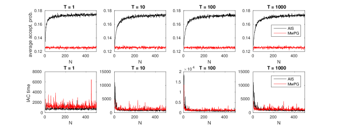
Figure 1: Average rate of acceptance and IAC time for the non-centred parametrisation of the model with informative observations.

We re-ran these experiments on a coarser grid of values of $(N,T)$, more precisely all the combinations of $T=10,100,1000,10000$ and $N=2,25,50,100,200$, but considered this time $200$ runs of the algorithm for each such combination. The results are reported in Figure 2 where we now also report in addition the ratios (MCMC AIS/MwPG) of the mean IAC times and mean square jump distances (multiplied by $T$). We see that the MCMC AIS algorithm is uniformly better in terms of MSJD, while MwPG seems to be superior for small values of $N$, but remind reader of the difficulty inherent to the estimation of IAC and note the presence of a significant number of outliers which indicate to us that the chains are not mixing well for such a range of values of $N$. The algorithms’ acceptance rates, not shown here, follow a very similar pattern to that observed for the mean square jumps.

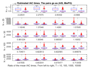
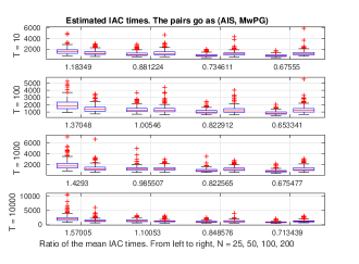
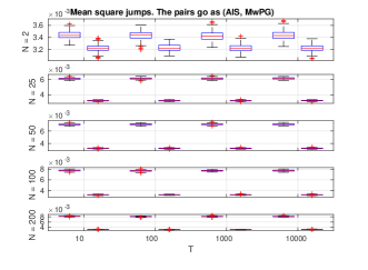
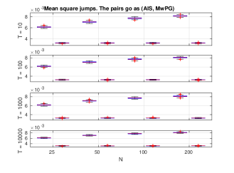
Figure 2: IAC times and mean square jumps (multiplied by $T$) for the hierarchical model for $a=1$. Ratios of the mean IAC times (MCMC AIS cSMC-BS/MwPG) are shown on the $x-$axis. On the right hand side plots, results for $N=2$ are not shown to improve legibility).

We re-ran these experiments for $a=0.1$, which is more favourable to the MwPG as this reduces the posterior dependence between $\theta$ and $x_{1:T}$. The results are presented in Figure 3. We observe that while MCMC AIS remains uniformly superior in terms of mean square jump distance (MSJD), as expected, the IAC ratios are now closer to one for large values of $N$, confirming that the wider gaps observed in our earlier experiments are attributable to the posterior dependence. This leads us to conclude that MCMC AIS is a more reliable method than MwPG when this dependence is a priori unknown.

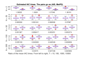
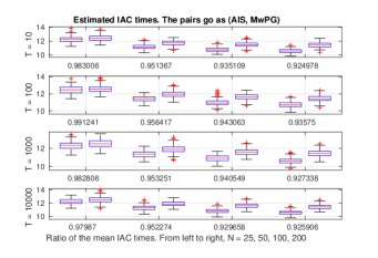
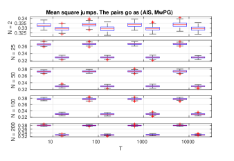
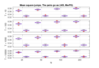
Figure 3: IAC times and mean square jumps (multiplied by $T$) for the hierarchical model for $a=0.1$. Ratios of the mean IAC times (MCMC AIS cSMC-BS/MwPG) are shown on the $x-$axis. On the right hand side plots, results for $N=2$ are not shown to improve readability).

5.2 Experiments on a non-linear state-space model

We consider now a non-linear SSM often used in the literature to compare the performance of SMC methods for which $f_{\theta}(x_{t-1},x_{t})=\mathcal{N}\big{(}x_{t};x_{t-1}/2+25x_{t-1}/(1+x_{t-1}^{2})+8\cos(1.2t),\sigma_{v}^{2}\big{)}$, $g_{\theta}(x_{t},y_{t})=\mathcal{N}\big{(}y_{t};x_{t}^{2}/20,\sigma_{w}^{2}\big{)}$ and $\mu_{\theta}(x_{1})=\mathcal{N}(x_{1};0,10)$. Here $\theta=(\sigma_{v}^{2},\sigma_{w}^{2})$ and the prior distribution was chosen to be $\sigma_{v}^{2},\sigma_{w}^{2}\overset{\texttt{{\rm iid}}}{\sim}\mathcal{IG}(0.01,0.01)$ where $\mathcal{IG}(a,b)$ is the inverse Gamma distribution with shape and scale parameters $a$ and $b$. Throughout the experiments, we generated data using the values $\sigma_{v}^{2}=100$ and $\sigma_{w}^{2}=1$

5.2.1 Comparison of algorithms for fixed $T$ and varying $N,K$

We first compare the performance of PMMH, MCMC AIS cSMC, MCMC AIS cSMC-BS and MwPG for fixed $T=500$ and various values of $K$ and $N$, for an approximately constant computational budget. To that purpose, for a given number of intermediate distributions $K$ we fix the number of particles to $N_{0}=500$ in the cSMC or cSMC-BS updates used to implement MCMC AIS, while we take the number of particles to be $N_{0}K$ for both the SMC and cSMC used within the PMMH and MwPG algorithms respectively. For the MCMC AIS algorithms, the intermediate distributions are chosen to be of the form $\gamma_{\theta,\theta^{\prime},k}=\gamma_{\theta_{k}}$, where $\theta_{k}=(1-\varsigma_{k})\theta+\varsigma_{k}\theta^{\prime}$, $\varsigma_{k}=k/(K+1)$, $k=0,\ldots,K+1$. Wherever an SMC or a cSMC routine is required for the implementation of the algorithms, multinomial resampling is used at every time step and the transition density of the SSM is used as the importance sampling distribution. We used a normal random walk proposal with diagonal covariance matrix for the RWM updates, where the standard deviation for $\sigma_{v}$ was $0.15$ and $0.08$ for $\sigma_{w}$. We report box plots of the IAC times associated to $\sigma_{v}^{2}$ and $\sigma_{w}^{2}$ in Figure 4 and average IAC times in Table 1. As observed earlier for the independent scenario the MwPG reaches its asymptotic regime for small values of $N$ and does not see its performance improve with the number of particles. This is in contrast with the PMMH and MCMC AIS cSMC-BS algorithms which achieve similar performance for large values of $K$ or $N$ and outperform the MwPG algorithm. We note the crucial role played by the backward sampling stage in the MCMC AIS algorithm and recall the reader here that the MwPG also relies on a cSMC-BS step.

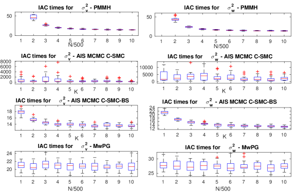
Figure 4: Box plots for the IAC times for $\sigma_{v}^{2}$ and $\sigma_{w}^{2}$ for algorithms PMMH, MCMC AIS cSMC, MCMC AIS cSMC-BS, and MwPG for various combinations of $N$ and $K$.

	MCMC AIS cSMC		MCMC AIS cSMC-BS		MwPG		PMMH
	$\sigma_{v}^{2}$	$\sigma_{w}^{2}$	$\sigma_{v}^{2}$	$\sigma_{w}^{2}$	$\sigma_{v}^{2}$	$\sigma_{w}^{2}$	$\sigma_{v}^{2}$	$\sigma_{w}^{2}$
$K=1$	44.9	657.2	17.7	20.9	22.9	29.8	161.9	309.3
$K=2$	74.3	3096.8	14.5	15.7	22.1	28.4	41.8	43.5
$K=3$	128.6	1960.0	13.9	15.6	22.8	28.1	22.6	21.6
$K=4$	114.0	1428.2	15.0	15.9	20.0	31.1	19.0	19.3
$K=5$	170.8	472.2	13.4	14.9	20.4	25.8	18.9	17.5
$K=6$	200.6	148.4	13.0	13.1	20.8	26.3	16.9	16.0
$K=7$	66.3	1733.6	13.7	12.4	18.3	26.5	16.6	14.1
$K=8$	638.9	544.5	13.7	12.6	22.7	27.6	14.3	13.7
$K=9$	122.2	1132.9	12.0	12.2	21.9	29.8	16.3	14.0
$K=10$	724.6	267.3	13.5	13.7	22.7	26.7	14.9	14.0

Table 1: Estimated IAC times for $\sigma_{v}^{2}$ and $\sigma_{w}^{2}$ for the algorithms considered. On each row the estimated IAC times for the MCMC AIS algorithms for $N_{0}=500$ particles and $K$ intermediate steps and MwG and PMMH algorithms for $N=KN_{0}$ particles are shown.

5.2.2 Comparison of algorithms for fixed $N$ and varying $T$

In a second experiment we compared PMMH, MCMC AIS cSMC-BS for $K=1$, and MwPG for varying values of $T$, in order to assess their scalability to the size of the observations. All the algorithms used the same number of particles in order to ensure comparable computational complexity. Each algorithm was run $200$ times with $N=200$ particles for $T=1000,2000,5000,10000$, with the exception of the PMMH for which $N=2000$, as otherwise the estimation of the IAC times was too unreliable, even for $T=1000$. The prior distribution and the other algorithm settings were similar to those of subsection 5.2.1. In Figure 5 we report the box plots for the IAC times estimated from the $200$ runs, while their averages are reported in Table 2. The PMMH algorithm clearly does not scale well as $T$ increases, in contrast with MCMC AIS cSMC-BS and MwPG which exhibit remarkable scaling properties, similar to those observed in the iid scenario. In line with our earlier findings, MCMC AIS cSMC-BS seems to be consistently marginally superior to MwPG, for a comparable computational cost.

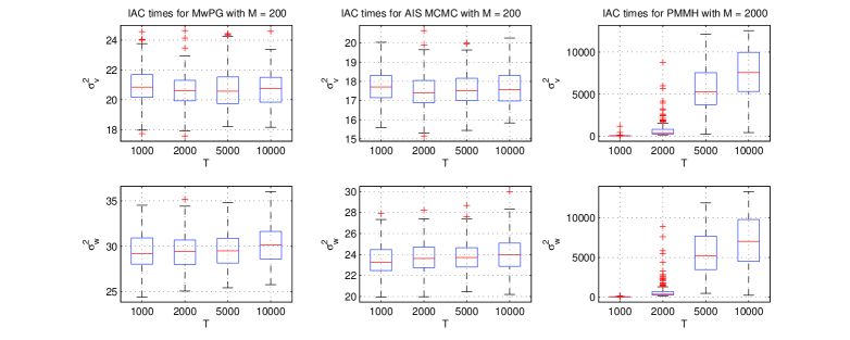
Figure 5: Box plots for the IAC times for $\sigma_{v}^{2}$ and $\sigma_{w}^{2}$ for MCMC AIS cSMC-BS and MwPG with $N=200$ and PMMH with $N=2000$. Mean IAC values are given in Table 2.

	MCMC AIS cSMC-BS		MwPG		PMMH
	$\sigma_{v}^{2}$	$\sigma_{w}^{2}$	$\sigma_{v}^{2}$	$\sigma_{w}^{2}$	$\sigma_{v}^{2}$	$\sigma_{w}^{2}$
$T=1000$	17.7	23.5	20.9	29.4	71.3	59.2
$T=2000$	17.5	23.7	20.6	29.4	759.0	757.9
$T=5000$	17.6	23.7	20.7	29.6	5808.6	5663.5
$T=10000$	17.6	24.0	20.7	30.2	7368.1	7170.9

Table 2: Estimated IAC times for $\sigma_{v}^{2}$ and $\sigma_{w}^{2}$ for MwPG and MCMC AIS cSMC-BS (with $K=1$) for $N=200$ and $N=2000$ for PMMH.

6 Discussion

We have introduced a novel likelihood ratio estimator for SSMs which relies on an original combination of AIS and cSMC and have shown how it can be used to obtain an MCMC algorithm to perform Bayesian parameter inference. In the i.i.d. case, we have provided theory for this estimator which suggests that the resulting MCMC algorithm has a computational cost at each iteration scaling linearly with $T$ instead of quadratically for standard pseudo-marginal methods. In the general SSM case, we conjecture that similar results also hold for the class of state-space models where cSMC-BS is efficient as evidenced by our empirical results.

Appendix A Approximation

We first establish a simple approximation of $\Lambda_{T}(\theta,\epsilon;\omega,\xi)$, which relies on a Taylor expansion. We let $\mathring{\Theta}$ be the interior of $\Theta$.

Lemma 1.

Assume (A(A3)). For any $(\theta,\epsilon,\xi,\omega)\in\mathring{\Theta}\times\Xi\times\mathsf{X}^{\mathbb{N}}\times\mathsf{Y}^{\mathbb{N}}$ and any $T\in\mathbb{N}$ such that $\tilde{\theta}(\epsilon,T)\in\mathring{\Theta}$ there exist $\{\mathring{\theta}_{t},1\leq t\leq T\},\{\bar{\theta}_{t},1\leq t\leq T\}\in[\theta\wedge\theta{}^{{}^{\prime}}(\epsilon,T),\theta\vee\theta{}^{{}^{\prime}}(\epsilon,T)]^{T}$ such that

$$\Lambda_{T}(\theta,\epsilon;\omega,\xi)=S_{\theta,\epsilon,T}^{(1)}(\omega,\xi)+S_{\theta,\epsilon,T}^{(2)}(\omega,\xi)+S_{\theta,\epsilon,T}^{(3)}(\omega,\xi)\quad.$$

with

$$S_{\theta,\epsilon,T}^{(1)}(\omega,\xi):=\frac{\epsilon}{2\sqrt{T}}\sum_{t=1}^{T}\left\{\dot{\ell}_{\theta}\big{(}x_{t}\mid y_{t}\big{)}+\dot{\ell}_{\tilde{\theta}(\epsilon,T)}\big{(}x^{\prime}_{t}\mid y_{t}\big{)}\right\},$$

$$S_{\theta,\epsilon,T}^{(2)}(\omega,\xi):=\frac{\epsilon^{2}}{8T}\sum_{t=1}^{T}\left\{\ddot{\ell}_{\theta}(x_{t}\mid y_{t})+\ddot{\ell}_{\tilde{\theta}(\epsilon,T)}(x^{\prime}_{t}\mid y_{t})\right\},$$

$$S_{\theta,\epsilon,T}^{(3)}(\omega,\xi):=\frac{\epsilon^{3}}{48T\sqrt{T}}\sum_{t=1}^{T}\left\{\dddot{\ell}_{\bar{\theta}_{t}}(x_{t}\mid y_{t})+\dddot{\ell}_{\mathring{\theta}_{t}}(x^{\prime}_{t}\mid y_{t})\right\}.$$

Proof.

Recall that

$$\Lambda_{T}(\theta,\epsilon;\omega,\xi) =\sum_{t=1}^{T}\log\frac{p_{\tilde{\theta}(\epsilon,T)}\left(x_{t}\mid y_{t}\right)}{p_{\theta}\left(x_{t}\mid y_{t}\right)}+\log\frac{p_{\theta^{\prime}(\epsilon,T)}\left(x^{\prime}_{t}\mid y_{t}\right)}{p_{\tilde{\theta}(\epsilon,T)}\left(x^{\prime}_{t}\mid y_{t}\right)}.$$

For $(\theta,\tilde{\theta})\in\mathring{\Theta}$ and $(x,y)\in\mathsf{X}\times\mathsf{Y}$ a Taylor expansion yields

$$\log\frac{p_{\tilde{\theta}}\left(x\mid y\right)}{p_{\theta}\left(x\mid y\right)} =\dot{\ell}_{\theta}(x\mid y)\big{(}\tilde{\theta}-\theta\big{)}+\frac{1}{2}\ddot{\ell}_{\theta}(x\mid y)\big{(}\tilde{\theta}-\theta\big{)}^{2}+\frac{1}{6}\dddot{\ell}_{\bar{\theta}}(x\mid y)\big{(}\tilde{\theta}-\theta\big{)}^{3}$$

for some $\bar{\theta}\in[\tilde{\theta}\wedge\theta^{\prime},\tilde{\theta}\vee\theta^{\prime}]$, also dependent on $x$ and $y$. Similarly for $(\tilde{\theta},\theta^{\prime})\in\mathring{\Theta}$

$$\log\frac{p_{\theta^{\prime}}\left(x\mid y\right)}{p_{\tilde{\theta}}\left(x\mid y\right)} =\dot{\ell}_{\tilde{\theta}}(x\mid y)\big{(}\theta^{\prime}-\tilde{\theta}\big{)}+\frac{1}{2}\ddot{\ell}_{\tilde{\theta}}(x\mid y)\big{(}\theta^{\prime}-\tilde{\theta}\big{)}^{2}+\frac{1}{6}\dddot{\ell}_{\mathring{\theta}}(x\mid y)\big{(}\theta^{\prime}-\tilde{\theta}\big{)}^{3}$$

for some $\mathring{\theta}\in[\tilde{\theta}\wedge\theta^{\prime},\tilde{\theta}\vee\theta^{\prime}]$, also dependent on $x$ and $y$. It follows that

$$\Lambda_{T}(\theta,\epsilon;\omega,\xi) =\sum_{t=1}^{T}\dot{\ell}_{\theta}(x_{t}\mid y_{t})\big{(}\tilde{\theta}(\epsilon,T)-\theta\big{)}+\dot{\ell}_{\tilde{\theta}(\epsilon,T)}(x^{\prime}_{t}\mid y_{t})\big{(}\theta^{\prime}(\epsilon,T)-\tilde{\theta}(\epsilon,T)\big{)}$$

$$+\frac{1}{2}\sum_{t=1}^{T}\ddot{\ell}_{\theta}(x_{t}\mid y_{t})\big{(}\tilde{\theta}(\epsilon,T)-\theta\big{)}^{2}+\ddot{\ell}_{\tilde{\theta}(\epsilon,T)}(x^{\prime}_{t}\mid y_{t})\big{(}\theta^{\prime}(\epsilon,T)-\tilde{\theta}(\epsilon,T)\big{)}^{2}$$

$$+\frac{1}{6}\sum_{t=1}^{T}\dddot{\ell}_{\bar{\theta}_{t}}(x_{t}\mid y_{t})\big{(}\tilde{\theta}(\epsilon,T)-\theta\big{)}^{3}+\dddot{\ell}_{\mathring{\theta}_{t}}(x^{\prime}_{t}\mid y_{t})\big{(}\theta^{\prime}(\epsilon,T)-\tilde{\theta}(\epsilon,T)\big{)}^{3}$$

Now, from the definition of $\tilde{\theta}(\epsilon,T)$ we have

$$\tilde{\theta}(\epsilon,T)-\theta:=\frac{\epsilon/2}{\sqrt{T}},\text{ }\theta^{\prime}(\epsilon,T)-\tilde{\theta}(\epsilon,T):=\frac{\epsilon/2}{\sqrt{T}},$$

and therefore

$$\Lambda_{T}(\theta,\epsilon;\omega,\xi) =\frac{\epsilon}{2\sqrt{T}}\sum_{t=1}^{T}\left\{\dot{\ell}_{\theta}(x_{t}\mid y_{t})+\dot{\ell}_{\tilde{\theta}(\epsilon,T)}(x^{\prime}_{t}\mid y_{t})\right\}$$

$$+\frac{\epsilon^{2}}{8T}\sum_{t=1}^{T}\left\{\ddot{\ell}_{\theta}(x_{t}\mid y_{t})+\ddot{\ell}_{\tilde{\theta}(\epsilon,T)}(x^{\prime}_{t}\mid y_{t})\right\}$$

$$+\frac{\epsilon^{3}}{48T\sqrt{T}}\sum_{t=1}^{T}\left\{\dddot{\ell}_{\bar{\theta}_{t}}(x_{t}\mid y_{t})+\dddot{\ell}_{\mathring{\theta}_{t}}(x^{\prime}_{t}\mid y_{t})\right\}.$$

∎

This is a purely technical lemma to establish various continuity properties needed after.

Lemma 2.

Assume (A(A3)). Then for any $(\theta,\theta^{\prime})\in\mathring{\Theta}^{2}$,

$$\sup_{y\in\mathsf{Y}}\|p_{\theta}(\cdot\mid y)-p_{\theta^{\prime}}(\cdot\mid y)\|_{tv}\leq\frac{1}{2}\bar{\ell}^{(1)}|\theta-\theta^{\prime}|.$$

Let $\phi_{\theta}(\cdot,\cdot):\Theta\times\mathsf{X}\times\mathsf{Y}\rightarrow\mathbb{R}$ and define $\bar{\phi}:=\sup_{(\theta,x,y)\in\Theta\times\mathsf{X}\times\mathsf{Y}}|\phi_{\theta}(x,y)|$. Then for any $(\theta,\epsilon,\omega)\in\Theta\times\Xi\times\mathsf{Y}^{\mathbb{N}}$, $T\geq 1$ and $N\in\mathbb{N}$

$$\left|\mathbb{E}_{\theta,\epsilon,T}^{\omega}\left[\phi_{\theta}(X{}_{1},y)\right]-\mathbb{E}_{\theta,\epsilon,T}^{\omega}\left[\phi_{\tilde{\theta}(\epsilon,T)}(X_{1}^{\prime},y)\right]\right|\leq\bar{\phi}\bar{\ell}^{(1)}\times\frac{|\epsilon|}{\sqrt{T}}\sup_{(\theta,x,y)\in\Theta\times\mathsf{X}\times\mathsf{Y}}\|R_{\theta,y}^{[N]}\big{(}x,\cdot\big{)}-p_{\theta}(\cdot\mid y)\|_{tv}\\ +\left|\mathbb{E}_{\tilde{\theta}(\epsilon,T)}^{\omega}\left[\phi_{\tilde{\theta}(\epsilon,T)}(X{}_{1},y)\right]-\mathbb{E}_{\theta}^{\omega}\left[\phi_{\theta}(X{}_{1},y)\right]\right|.$$

If in addition there exists $\tilde{\phi}>0$ such that for all $(\theta,\theta^{\prime},x,y)\in\mathring{\Theta}^{2}\times\mathsf{X}\times\mathsf{Y}$, $|\phi_{\theta}(x,y)-\phi_{\theta^{\prime}}(x,y)|\leq\tilde{\phi}|\theta-\theta^{\prime}|$ then

$$\left|\mathbb{E}_{\theta^{\prime}}^{\omega}\left[\phi_{\theta^{\prime}}(X{}_{1},y)\right]-\mathbb{E}_{\theta}^{\omega}\left[\phi_{\theta}(X{}_{1},y)\right]\right|\leq(\bar{\phi}\bar{\ell}^{(1)}+\tilde{\phi})|\theta-\theta^{\prime}|.$$

Proof.

We have for any $y\in\mathsf{Y}$

$$\|p_{\theta}(\cdot \mid y)-p_{\theta^{\prime}}(\cdot\mid y)\|_{tv}=\frac{1}{2}\int_{\mathsf{X}}|\exp(\ell_{\theta}(x\mid y))-\exp(\ell_{\theta^{\prime}}(x\mid y))|{\rm d}x$$

$$=\frac{1}{2}\int_{\mathsf{X}}|\int_{\theta}^{\theta^{\prime}}\dot{\ell}_{\vartheta}(x\mid y)\exp(\ell_{\vartheta}(x\mid y)){\rm d}\vartheta|{\rm d}x$$

$$\leq\frac{1}{2}\bar{\ell}^{(1)}|\int_{\theta}^{\theta^{\prime}}\int_{\mathsf{X}}\exp(\ell_{\vartheta}(x\mid y)){\rm d}x{\rm d}\vartheta|$$

$$=\frac{1}{2}\bar{\ell}^{(1)}|\theta-\theta^{\prime}|.$$

For the next statement we use standard operator notation for brevity: for a probability distribution $\mu$, a Markov operator $\Pi$ and a function $f$, we let $\Pi f(x):=\int f(u)\Pi(x,{\rm d}u)$ and $\mu f=\mu(f):=\int f(u)\mu({\rm d}u)$. We have the decomposition, for $\theta,\tilde{\theta}\in\Theta$ and $N\in\mathbb{N}$

$$p_{\theta}R_{\tilde{\theta},y}^{[N]}\left(\phi_{\tilde{\theta}}\right)-p_{\theta}\left(\phi_{\theta}\right) =p_{\theta}R_{\tilde{\theta},y}^{[N]}\left(\phi_{\tilde{\theta}}\right)-p_{\tilde{\theta}}R_{\tilde{\theta},y}^{[N]}\left(\phi_{\tilde{\theta}}\right)+p_{\tilde{\theta}}\left(\phi_{\tilde{\theta}}\right)-p_{\theta}\left(\phi_{\theta}\right)$$

$$=(p_{\theta}-p_{\tilde{\theta}})R_{\tilde{\theta},y}^{[N]}(\phi_{\tilde{\theta}}-p_{\tilde{\theta}}\phi_{\tilde{\theta}})+(p_{\tilde{\theta}}-p_{\theta})\left(\phi_{\tilde{\theta}}\right)-p_{\theta}(\phi_{\theta}-\phi_{\tilde{\theta}})$$

and

$$|(p_{\theta}-p_{\tilde{\theta}})R_{\tilde{\theta},y}^{[N]}(\phi_{\tilde{\theta}}-p_{\tilde{\theta}}\phi_{\tilde{\theta}})| \leq 2\|p_{\theta}-p_{\tilde{\theta}}\|_{tv}\sup_{x\in\mathsf{X}}|R_{\tilde{\theta},y}^{[N]}(\phi_{\tilde{\theta}}-p_{\tilde{\theta}}\phi_{\tilde{\theta}})(x)|$$

$$\leq 2\|p_{\theta}-p_{\tilde{\theta}}\|_{tv}2\sup_{x\in\mathsf{X}}\|R_{\tilde{\theta},y}^{[N]}(x,\cdot)-p_{\tilde{\theta}}(\cdot\mid y)\|_{tv}\bar{\phi}.$$

Finally we have the decomposition and bound for $\theta,\theta^{\prime}\in\mathring{\Theta}$

$$\left|(p_{\theta^{\prime}}-p_{\theta})\left(\phi_{\theta^{\prime}}\right)-p_{\theta}(\phi_{\theta}-\phi_{\theta^{\prime}})\right| \leq 2\bar{\phi}\|p_{\theta}(\cdot\mid y)-p_{\theta^{\prime}}(\cdot\mid y)\|_{tv}+\tilde{\phi}|\theta-\theta^{\prime}|$$

$$=(\bar{\phi}\bar{\ell}^{(1)}+\tilde{\phi})|\theta-\theta^{\prime}|.$$

∎

We establish a first level of approximation of $\Lambda_{T}(\theta,\epsilon;\omega,\xi)$ in the following sense.

Lemma 3.

Assume (A(A3)). For any $(\theta,\epsilon,\omega,T)\in\Theta\times\Xi\times\mathsf{Y}^{\mathbb{N}}\times\mathbb{N}$, let

$$\bar{S}_{\theta,T}^{(2)}(\omega):=\frac{\epsilon^{2}}{4T}\sum_{t=1}^{T}\mathbb{E}_{\theta}^{\omega}\big{[}\ddot{\ell}_{\theta}(X_{t}\mid y_{t})\big{]}.$$

Then for any $\omega\in\mathsf{Y}^{\mathbb{N}}$ and with the notation of Lemma 1,

$$\lim_{T\rightarrow\infty}\sup_{(N_{T},\theta,\epsilon)\in\mathbb{N}\times\mathring{\Theta}\times\Xi}\mathbb{E}_{\theta,\epsilon,T}^{\omega}\big{|}\Lambda_{T}(\theta,\epsilon;\omega,\xi)-S_{\theta,\epsilon,T}^{(1)}(\omega,\xi)-\bar{S}_{\theta,\epsilon,T}^{(2)}(\omega)\big{|}=0.$$

Proof.

First we have

$$\Lambda_{T}(\theta,\epsilon)-S_{\theta,\epsilon,T}^{(1)}(\omega,\xi)-\bar{S}_{\theta,\epsilon,T}^{(2)}(\omega,\xi)=S_{\theta,\epsilon,T}^{(2)}(\omega,\xi)-\bar{S}_{\theta,\epsilon,T}^{(2)}(\omega)+S_{\theta,\epsilon,T}^{(3)}(\omega,\xi)$$

and we are going to consider the second order moment of the term on the right hand side–we will then invoke the standard inequality ${\rm\mathbb{E}}_{\theta,\epsilon,T}^{\omega}|Z|\leq\sqrt{{\rm\mathbb{E}}_{\theta,\epsilon,T}^{\omega}[Z^{2}]}$ in order to conclude. In order to alleviate notation we introduce $\|Z\|_{2}:=\sqrt{{\rm\mathbb{E}}_{\theta,\epsilon,T}^{\omega}\left(Z^{2}\right)}$, which satisfies the triangle inequality, and drop the dependence on $\omega$. We bound $\|S_{\theta,\epsilon,T}^{(3)}\|_{2}$ and $\|S_{\theta,\epsilon,T}^{(2)}-\bar{S}_{\theta,\epsilon,T}^{(2)}\|_{2}$. Clearly we have

$$\|S_{\theta,\epsilon,T}^{(3)}\|_{2}\leq\frac{|\epsilon|^{3}}{48\sqrt{T}}2\bar{\ell}^{(3)}\quad.$$

Now define

$$\tilde{S}_{\theta,\epsilon,T}^{(2)}:=\frac{\epsilon^{2}}{8T}\sum_{t=1}^{T}\left\{\mathbb{E}_{\theta,\epsilon,T}^{\omega}[\ddot{\ell}_{\theta}(X_{t}\mid y_{t})+\ddot{\ell}_{\tilde{\theta}(\epsilon,T)}(X^{\prime}_{t}\mid y_{t})]\right\}$$

and consider the upper bound

$$\|S_{\theta,\epsilon,T}^{(2)}-\bar{S}_{\theta,\epsilon,T}^{(2)}\|_{2}\leq\|S_{\theta,\epsilon,T}^{(2)}-\tilde{S}_{\theta,\epsilon,T}^{(2)}\|_{2}+\|\tilde{S}_{\theta,\epsilon,T}^{(2)}-\bar{S}_{\theta,\epsilon,T}^{(2)}\|_{2}.$$

Using independence we obtain

$$\|S_{\theta,\epsilon,T}^{(2)}-\tilde{S}_{\theta,\epsilon,T}^{(2)}\|_{2} =\frac{\epsilon^{2}}{8T}\sqrt{\sum_{t=1}^{T}{\rm\mathbb{V}}_{\theta,\epsilon,T}^{\omega}\left(\ddot{\ell}_{\theta}(X_{t}\mid y_{t})+\ddot{\ell}_{\tilde{\theta}(\epsilon,T)}(X^{\prime}_{t}\mid y_{t})\right)}$$

$$\leq\frac{\epsilon^{2}}{4\sqrt{T}}\bar{\ell}^{(2)}.$$

Finally

$$\|\tilde{S}_{\theta,\epsilon,T}^{(2)}-\bar{S}_{\theta,\epsilon,T}^{(2)}\|_{2} =\frac{\epsilon^{2}}{8T}\|\sum_{t=1}^{T}\left\{\mathbb{E}_{\theta,\epsilon,T}^{\omega}[\ddot{\ell}_{\theta}(X_{t}\mid y_{t})-\ddot{\ell}_{\tilde{\theta}(\epsilon,T)}(X^{\prime}_{t}\mid y_{t})]\right\}\|_{2}.$$

The estimate of the difference obtained in Lemma 2 leads to

$$|\mathbb{E}_{\theta,\epsilon,T}^{\omega}[\ddot{\ell}_{\theta}(X_{t}\mid y_{t})-\ddot{\ell}_{\tilde{\theta}(\epsilon,T)}(X^{\prime}_{t}\mid y_{t})]|\\ \leq\bar{\ell}^{(1)}\bar{\ell}^{(2)}\frac{|\epsilon|}{\sqrt{T}}\sup_{(\theta,x,y)\in\mathring{\Theta}\times\mathsf{X}\times\mathsf{Y}}\|R_{\theta,y}^{[N_{T}]}\big{(}x,\cdot\big{)}-p_{\theta}(\cdot\mid y)\|_{tv}+(\bar{\ell}^{(1)}\bar{\ell}^{(2)}+\bar{\ell}^{(3)})\frac{|\epsilon|}{2\sqrt{T}}$$

and we conclude since the total variation term is bounded by $1$. ∎

The following result establishes that $P-a.s.$ one can approximate $\Lambda_{T}(\theta,\epsilon;\omega,\xi)$ with $S_{\theta,\epsilon,T}^{(1)}(\omega,\xi)-\sigma^{2}(\theta,\epsilon)/2$ in the sense given in the corollary below.

Lemma 4.

Assume (A(A3)), then

$$\lim_{T\rightarrow\infty}\sup_{(N_{T},\theta,\epsilon)\in\mathbb{N}\times\Theta\times\Xi}\big{|}\bar{S}_{\theta,\epsilon,T}^{(2)}(\omega)-\frac{\epsilon^{2}}{4}\mathbb{E_{\theta}}\big{[}\ddot{\ell}_{\theta}(X_{1}\mid Y_{1})\big{]}\big{|}=0\quad P-a.s.$$

Proof.

We use a straightforward adaptation of the simple result of Tauchen (1985, Lemma 1). Conditions (iii) and (iv) of Tauchen (1985, Lemma 1) are immediate since for any $\omega\in\mathsf{Y}^{\mathbb{N}}$, $(\theta,\epsilon)\mapsto\epsilon^{2}\mathbb{E}_{\theta}^{\omega}\big{[}\ddot{\ell}_{\theta}\big{(}X{}_{1}\mid y\big{)}\big{]}$ is continuous from Lemma 2 and $\Theta\times\Xi$ is assumed compact, implying $\sup_{(\theta,\epsilon)\in\Theta\times\Xi}|\epsilon^{2}\mathbb{E}_{\theta}^{\omega}\big{[}\ddot{\ell}_{\theta}\big{(}X{}_{1}\mid y\big{)}\big{]}|\leq\ddot{\ell}^{(2)}\sup_{\epsilon\in\Xi}\epsilon^{2}<\infty$, which is obviously integrable w.r.t the distribution of the observations. We are left with establishing the measurability of the suprema considered, covered by (ii) of Tauchen (1985, Lemma 1). Note that if for any $y_{1:T}\in\mathsf{Y}^{T}$ $(\theta,\epsilon)\mapsto\phi(\theta,\epsilon,y_{1:T})$ is continuous then

$$y_{1:T}\mapsto\sup_{(\theta,\epsilon)\in\Theta\times\Xi}\phi(\theta,\epsilon,y_{1:T})=\sup_{(\theta,\epsilon)\in(\Theta\times\Xi)\cap\mathbb{Q}^{2}}\phi(\theta,\epsilon,y_{1:T})$$

is measurable. Since for any $y\in\mathsf{Y}$, $(\theta,\epsilon)\mapsto\epsilon^{2}\mathbb{E}_{\theta}^{\omega}\big{[}\ddot{\ell}_{\theta}\big{(}X{}_{1}\mid y\big{)}\big{]}$ is continuous by Lemma 2, we conclude. ∎

Corollary 1.

Recalling that $\sigma^{2}(\theta,\epsilon):=\frac{-\epsilon^{2}}{2}\mathbb{E}_{\theta}\left[\ddot{\ell}_{\theta}(X_{1}\mid Y_{1})\right]$, $P-a.s.$ we have

$$\lim_{T\rightarrow\infty}\sup_{(N_{T},\theta,\epsilon)\in\mathbb{N}\times\mathring{\Theta}\times\Xi}\mathbb{E}_{\theta,\epsilon,T}^{\omega}\big{|}\Lambda_{T}(\theta,\epsilon;\omega,\xi)-S_{\theta,\epsilon,T}^{(1)}(\omega,\xi)+\sigma^{2}(\theta,\epsilon)/2\big{|}=0.$$

We now seek to establish that $S_{\theta,\epsilon,T}^{(1)}(\omega,\xi)$ satisfies a $(\theta,\epsilon)$-uniform central limit theorem (U-CLT) with limiting mean and variance $P-a.s.$ independent of $\omega$.

Appendix B Conditional CLT for $S_{\theta,\epsilon,T}^{(1)}(\xi,\omega)$

We now apply a CLT conditional upon the observations and will notice that $P-$a.s. the constants involved are asymptotically independent of the realisation of the observations.

B.1 Checking Lyapunov’s theorem conditions

We will use the following technical lemma

Lemma 5.

Assume (A(A3)). Then for any $(\theta,\epsilon)\in\mathring{\Theta}\times\Xi$, $T\geq 1$, $N_{T}\in\mathbb{N}$ and $\omega\in\mathsf{Y}^{\mathbb{N}}$

$$\left|\mathbb{C}_{\theta,\epsilon,T}^{\omega}\left[\dot{\ell}_{\theta}(X_{t}\mid y_{t}),\dot{\ell}_{\tilde{\theta}(\epsilon,T)}(X^{\prime}_{t}\mid y_{t})\right]\right|\leq\sup_{(\theta,x,y)\in\Theta\times\mathsf{X}\times\mathsf{Y}}\|R_{\theta,y}^{[N_{T}]}(x,\cdot)-p_{\theta}(\cdot\mid y)\|_{tv}\times\big{(}\bar{\ell}^{(1)}\big{)}^{2}\left[1+\bar{\ell}^{(1)}\times\frac{|\epsilon|}{\sqrt{T}}\right].$$

Further for any $t\geq 1$ we have

$$\lim_{T\rightarrow\infty}\sup_{(N_{T},\theta,\epsilon,y_{t})\in\mathbb{N}\times\mathring{\Theta}\times\Xi\times\mathsf{Y}}\left|\mathbb{V}_{\theta,\epsilon,T}^{\omega}\left[\dot{\ell}_{\tilde{\theta}(\epsilon,T)}\big{(}X^{\prime}_{t}\mid y_{t}\big{)}\right]-\mathbb{V}_{\theta}^{y}\left[\dot{\ell}_{\theta}(X{}_{t}\mid y_{t})\right]\right|=0.$$

Proof.

First note that $\mathbb{E}_{\tilde{\theta}(\epsilon,T)}^{\omega}\big{[}\dot{\ell}_{\tilde{\theta}(\epsilon,T)}(X{}_{t}\mid y_{t})\big{]}=0$ and $\mathbb{E}_{\theta}^{\omega}\left[\dot{\ell}_{\theta}(X_{t}\mid y_{t})\right]=0$ and apply the Cauchy-Schwartz inequality to obtain

$$\left|\mathbb{E}_{\theta,\epsilon,T}^{\omega}\left[\dot{\ell}_{\theta}(X_{t}\mid y_{t})\mathbb{E}_{\theta,\epsilon,T}^{\omega}\big{[}\dot{\ell}_{\tilde{\theta}(\epsilon,T)}(X^{\prime}_{t}\mid y_{t})-\mathbb{E}_{\tilde{\theta}(\epsilon,T)}^{\omega}\big{[}\dot{\ell}_{\tilde{\theta}(\epsilon,T)}(X{}_{t}\mid y_{t})\big{]}\mid X_{t}\big{]}\right]\right|\leq\\ \sqrt{\sup_{(\theta,y_{t})\in\mathring{\Theta}\times\mathsf{Y}}\mathbb{V}_{\theta}^{\omega}\left[\dot{\ell}_{\theta}(X{}_{t}\mid y_{t})\right]}\times 2\bar{\ell}^{(1)}\sup_{(\theta,x,y)\in\mathring{\Theta}\times\mathsf{X}\times\mathsf{Y}}\|R_{\theta,y}^{[N_{T}]}(x,\cdot)-p_{\theta}(\cdot\mid y)\|_{tv}.$$ (11)

For the second statement, it is sufficient to show that for $\gamma\in\{1,2\}$

$$\lim_{T\rightarrow\infty}\sup_{(\theta,\epsilon,y_{t})\in\mathring{\Theta}\times\Xi\times\mathsf{Y}}\left|\mathbb{E}_{\theta}^{\omega}\left[\dot{\ell}_{\tilde{\theta}(\epsilon,T)}^{\gamma}(X^{\prime}_{t}\mid y_{t})\right]-\mathbb{E}_{\theta}^{\omega}\left[\dot{\ell}_{\theta}^{\gamma}(X{}_{t}\mid y_{t})\right]\right|=0.$$

The case $\gamma=1$ is treated in the proof of Lemma 7. For $\gamma=2$ we again use Lemma 2 and get the bound

$$|\mathbb{E}_{\theta,\epsilon,T}^{\omega}[\dot{\ell}_{\theta}^{2}(X_{t}\mid y_{t})-\dot{\ell}_{\tilde{\theta}(\epsilon,T)}^{2}(X^{\prime}_{t}\mid y_{t})]|\\ \leq\big{(}\bar{\ell}^{(1)}\big{)}^{3}\frac{|\epsilon|}{\sqrt{T}}\sup_{(\theta,x,y)\Theta\times\mathsf{X}\times\mathsf{Y}}\|R_{\theta,y}^{[N_{T}]}\big{(}x,\cdot\big{)}-p_{\theta}(\cdot\mid y)\|_{tv}+(\big{(}\bar{\ell}^{(1)}\big{)}^{3}+2\bar{\ell}^{(1)}\bar{\ell}^{(2)})\frac{|\epsilon|}{2\sqrt{T}}.$$

∎

Corollary 2.

Under (A(A3)) there exists $N_{0},T_{0}\in\mathbb{N}$ such that for any $\big{\{}N_{T}\big{\}}$ such that $\liminf_{T\rightarrow\infty}N_{T}\geq N_{0}$ then

$$\sup_{T\geq T_{0}}\sup_{(\theta,\epsilon,y_{t})\in\mathring{\Theta}\times\Xi\times\mathsf{Y}}\frac{\left|\mathbb{C}_{\theta,\epsilon,T}^{\omega}\left[\dot{\ell}_{\theta}(X_{t}\mid y_{t}),\dot{\ell}_{\tilde{\theta}(\epsilon,T)}(X^{\prime}_{t}\mid y_{t})\right]\right|}{\sqrt{\mathbb{V}_{\theta}^{\omega}\left(\dot{\ell}_{\theta}\big{(}X_{t}\mid y_{t}\big{)}\right)\mathbb{V}_{\theta,\epsilon,T}^{\omega}\left(\dot{\ell}_{\tilde{\theta}(\epsilon,T)}\big{(}X^{\prime}_{t}\mid y_{t}\big{)}\right)}}<1,$$

implying that the first condition of Lemma 6 below holds.

Lemma 6.

Assume (A(A3)) and let $\big{\{}N_{T}\big{\}}\in\mathbb{N}$ be such that for some $T_{0}\in\mathbb{N}$

$$\inf_{T\geq T_{0}}\inf_{(\theta,\epsilon,y_{t})\in\mathring{\Theta}\times\Xi\times\mathsf{Y}}\frac{\mathbb{C}_{\theta,\epsilon,T}^{\omega}\left[\dot{\ell}_{\theta}(X_{t}\mid y_{t}),\dot{\ell}_{\tilde{\theta}(\epsilon,T)}(X^{\prime}_{t}\mid y_{t})\right]}{\sqrt{\mathbb{V}_{\theta}^{\omega}\left(\dot{\ell}_{\theta}\big{(}X_{t}\mid y_{t}\big{)}\right)\mathbb{V}_{\theta,\epsilon,T}^{\omega}\left(\dot{\ell}_{\tilde{\theta}(\epsilon,T)}\big{(}X^{\prime}_{t}\mid y_{t}\big{)}\right)}}>-1.$$ (12)

Let $S_{\theta,\epsilon,T}^{(1)}(\omega,\xi)$ be as defined in Lemma 1 and let for any $(\theta,\epsilon)\in\mathring{\Theta}\times\Xi$ and $\omega\in\mathsf{Y}^{\mathbb{N}}$

$$\bar{S}_{\theta,\epsilon,T}^{(1)}(\omega):=\frac{\epsilon}{2\sqrt{T}}\sum_{t=1}^{T}\mathbb{E}_{\theta,\epsilon,T}^{\omega}\big{[}\dot{\ell}_{\tilde{\theta}(\epsilon,T)}\big{(}X^{\prime}_{t}\mid y_{t}\big{)}\big{]}$$

and

$$\sigma_{T}^{2}(\theta,\epsilon;\omega):=\frac{\epsilon^{2}}{4T}\sum_{t=1}^{T}\mathbb{V}_{\theta,\epsilon,T}^{\omega}\left\{\dot{\ell}_{\theta}(X_{t}\mid y_{t})+\dot{\ell}_{\tilde{\theta}(\epsilon,T)}(X^{\prime}_{t}\mid y_{t})\right\}.$$

Then for any $\omega\in\mathsf{Y}^{\mathbb{N}}$,

$$\lim_{T\rightarrow\infty}\sup_{(\theta,\epsilon,z)\in\mathring{\Theta}\times\Xi\times\mathbb{R}}\left|\mathbb{P}_{\theta,\epsilon,T}^{\omega}\left(\tfrac{S_{\theta,\epsilon,T}^{(1)}(\xi,\omega)-\bar{S}_{\theta,\epsilon,T}^{(1)}(\omega)}{\sigma_{T}(\theta,\epsilon;\omega)}\leq z\right)-\Phi(z)\right|=0,$$

where $\Phi(\cdot)$ is the cumulative distribution function of $\mathcal{N}(0,1)$.

Proof.

For $\delta>0$ let

$$N_{\theta,\epsilon,T}^{\omega}:=\sum_{t=1}^{T}\mathbb{E}_{\theta,\epsilon,T}^{\omega}\left[\left|\dot{\ell}_{\theta}(X_{t}\mid y_{t})+\dot{\ell}_{\tilde{\theta}(\epsilon,T)}\big{(}X^{\prime}_{t}\mid y_{t}\big{)}-\mathbb{E}_{\theta}^{\omega}\big{[}\dot{\ell}_{\tilde{\theta}(\epsilon,T)}\big{(}X^{\prime}_{t}\mid y_{t}\big{)}\big{]}\right|^{2+\delta}\right]$$

and

$$D_{\theta,\epsilon,T}^{\omega}:=\left({\textstyle\sum}_{t=1}^{T}\mathbb{V}_{\theta,\epsilon,T}^{\omega}\big{(}\dot{\ell}_{\theta}\big{(}X_{t}\mid y_{t}\big{)}+\dot{\ell}_{\tilde{\theta}(\epsilon,T)}\big{(}X^{\prime}_{t}\mid y_{t}\big{)}\big{)}\right)^{1+\delta/2}.$$

Lyapunov’s theorem (Petrov, 1995, Theorem 5.7, p. 154) states that there exists a universal constant $C$ such that for any $T\in\mathbb{N}$

$$\sup_{z\in\mathbb{R}}\left|\mathbb{P}_{\theta,\epsilon,T}^{\omega}\left(\tfrac{S_{\theta,\epsilon,T}^{(1)}(\xi,\omega)-\bar{S}_{\theta,\epsilon,T}^{(1)}(\omega)}{\sigma_{T}(\theta,\epsilon;\omega)}\leq z\right)-\Phi(z)\right|\leq C\frac{N_{\theta,\epsilon,T}^{\omega}}{D_{\theta,\epsilon,T}^{\omega}}.$$

In order to establish our uniform result we will check that we have $(\theta,\epsilon)-$uniform convergence of the upper bound. Clearly

$$N_{\theta,\epsilon,T}^{\omega}\leq 3^{2+\delta}\bar{\ell}^{(1)}T$$

and

$$D_{\theta,\epsilon,T}^{\omega}\geq T^{1+\delta/2}\left\{\inf_{(\theta,\epsilon,T,y_{t})\in\mathring{\Theta}\times\Xi\times\mathbb{N}\times\mathsf{Y}}\mathbb{V}_{\theta,\epsilon,T}^{\omega}\left(\dot{\ell}_{\theta}\big{(}X_{t}\mid y_{t}\big{)}+\dot{\ell}_{\tilde{\theta}(\epsilon,T)}\big{(}X^{\prime}_{t}\mid y_{t}\big{)}\right)\right\}^{1+\delta/2}.$$

If $\inf_{(\theta,\epsilon,T,y_{t})\in\mathring{\Theta}\times\Xi\times\mathbb{N}\times\mathsf{Y}}\mathbb{V}_{\theta,\epsilon,T}^{\omega}\left(\dot{\ell}_{\theta}\big{(}X_{t}\mid y_{t}\big{)}+\dot{\ell}_{\tilde{\theta}(\epsilon,T)}\big{(}X^{\prime}_{t}\mid y_{t}\big{)}\right)>0$ then the denominator grows super linearly and we can conclude. We have

$$\mathbb{V}_{\theta,\epsilon,T}^{\omega}\left(\dot{\ell}_{\theta}\big{(}X_{t}\mid y_{t}\big{)}+\dot{\ell}_{\tilde{\theta}(\epsilon,T)}\big{(}X^{\prime}_{t}\mid y_{t}\big{)}\right)\\ \geq 2\sqrt{\mathbb{V}_{\theta}^{\omega}\left(\dot{\ell}_{\theta}\big{(}X_{t}\mid y_{t}\big{)}\right)\mathbb{V}_{\theta,\epsilon,T}^{\omega}\left(\dot{\ell}_{\tilde{\theta}(\epsilon,T)}\big{(}X^{\prime}_{t}\mid y_{t}\big{)}\right)}+2\mathbb{C}_{\theta,\epsilon,T}^{\omega}\left[\dot{\ell}_{\theta}(X_{t}\mid y_{t}),\dot{\ell}_{\tilde{\theta}(\epsilon,T)}(X^{\prime}_{t}\mid y_{t})\right]$$

and conclude using the second part of Lemma 5, the assumption in (12) and the fact that by (A(A3)) we have $\inf_{(\theta,\epsilon,y_{t})\in\Theta\times\Xi\times\mathsf{Y}}\mathbb{V}_{\theta}^{\omega}\left(\dot{\ell}_{\theta}\big{(}X_{t}\mid y_{t}\big{)}\right)>0$. ∎

Remark 6.

The assumption in (12) will be satisfied whenever $R_{\theta,y}^{[N]}\big{(}x,\cdot\big{)}$ is a positive operator, or can be checked using Corollary 2.

We now examine the limits as $T\rightarrow\infty$ of $\bar{S}_{\theta,\epsilon,T}^{(1)}(\omega)$ and $\sigma_{T}^{2}(\theta,\epsilon;\omega)$ under the distribution of the observations $P$.

B.2 Limit of the expectations in the conditional CLT

Lemma 7.

Assume (A(A3)). Then with the notation from Lemma 6, for any $\varepsilon_{0}>0$ there exists $N_{0}\in\mathbb{N}$ such that

$$\sup_{T\geq 1}\sup_{(\theta,\epsilon,\omega)\in\mathring{\Theta}\times\Xi\times\mathsf{Y}^{\mathbb{N}}}\left|\bar{S}_{\theta,\epsilon,T}^{(1)}(\omega)\right|\mathbb{I}\{N_{T}\geq N_{0}\}\leq\varepsilon_{0}.$$

Proof.

We apply the result of Lemma 2 and use the fact that here for any $\theta\in\Theta$ and $t\geq 1$ we have $\mathbb{E}_{\theta}^{\omega}\big{[}\dot{\ell}_{\theta}(X_{t}\mid y_{t})\big{]}=0$. Therefore for any $t\geq 1$ and $(\theta,\epsilon,y_{t})\in\mathring{\Theta}\times\Xi\times\mathsf{Y}$,

$$\left|\mathbb{E}_{\theta}^{\omega}\left[\dot{\ell}_{\theta}(X{}_{t}\mid y_{t})\right]-\mathbb{E}_{\theta,\epsilon,T}^{\omega}\left[\dot{\ell}_{\tilde{\theta}(\epsilon,T)}(X^{\prime}_{t}\mid y_{t})\right]\right|\leq\big{(}\bar{\ell}^{(1)}\big{)}^{2}\times\frac{|\epsilon|}{\sqrt{T}}\sup_{(\theta,x,y)\Theta\times\mathsf{X}\times\mathsf{Y}}\|R_{\theta,y}^{[N_{T}]}\big{(}x,\cdot\big{)}-p_{\theta}(\cdot\mid y)\|_{tv}.$$

Hence

$$\left|\bar{S}_{\theta,\epsilon,T}^{(1)}\right|\leq\frac{|\epsilon|}{2}\big{(}\bar{\ell}^{(1)}\big{)}^{2}\sup_{(\theta,x,y)\in\Theta\times\mathsf{X}\times\mathsf{Y}}\|R_{\theta,y}^{[N_{T}]}\big{(}x,\cdot\big{)}-p_{\theta}(\cdot\mid y)\|_{tv},$$

and we conclude with the increasing ergodicity of $R_{\theta,y}^{[N]}\big{(}x,\cdot\big{)}$ with $N$. ∎

B.3 Limit of the variances in the conditional CLT

Lemma 8.

Assume (A(A3)). Then for any $\varepsilon_{0}>0$ there exists $T_{0},N_{0}\in\mathbb{N}$ such that

$$\sup_{T\geq T_{0}}\sup_{(\theta,\epsilon)\in\mathring{\Theta}\times\Xi}\left|\sigma_{T}^{2}(\theta,\epsilon;\omega)-\sigma^{2}(\theta,\epsilon)\right|\mathbb{I}\{N_{T}\geq N_{0}\}\leq\varepsilon_{0}\quad P-a.s.$$

Proof.

Note that for any $t\geq 1$

$$\mathbb{V}_{\theta,\epsilon,T}^{\omega}\left(\dot{\ell}_{\theta}\big{(}X_{t}\mid y_{t}\big{)}+\dot{\ell}_{\tilde{\theta}(\epsilon,T)}\big{(}X^{\prime}_{t}\mid y_{t}\big{)}\right)\\ =\mathbb{V}_{\theta}^{\omega}\left(\dot{\ell}_{\theta}\big{(}X_{t}\mid y_{t}\big{)}\right)+\mathbb{V}_{\theta,\epsilon,T}^{\omega}\left(\dot{\ell}_{\tilde{\theta}(\epsilon,T)}\big{(}X^{\prime}_{t}\mid y_{t}\big{)}\right)+2\mathbb{C}_{\theta,\epsilon,T}^{\omega}\left[\dot{\ell}_{\theta}(X_{t}\mid y_{t}),\dot{\ell}_{\tilde{\theta}(\epsilon,T)}(X^{\prime}_{t}\mid y_{t})\right].$$

From Lemma 5 and (A(A3)) there exist $T_{0,1},N_{0}\in\mathbb{N}$ such that for $T\geq T_{0,1}$ and $N_{T}\geq N_{0}$

$$\sup_{(\theta,\epsilon,y_{t})\in\mathring{\Theta}\times\Xi\times\mathsf{Y}}\left|\mathbb{C}_{\theta,\epsilon,T}^{\omega}\big{[}\dot{\ell}_{\theta}(X_{t}\mid y_{t}),\dot{\ell}_{\tilde{\theta}(\epsilon,T)}(X^{\prime}_{t}\mid y_{t})\big{]}\right|+\left|\mathbb{V}_{\theta,\epsilon,T}^{\omega}\left(\dot{\ell}_{\theta}\big{(}X_{t}\mid y_{t}\big{)}\right)-\mathbb{V}_{\theta,\epsilon,T}^{\omega}\left(\dot{\ell}_{\tilde{\theta}(\epsilon,T)}\big{(}X^{\prime}_{t}\mid y_{t}\big{)}\right)\right|\leq\varepsilon_{0}/4$$

Therefore, since $\sup_{(\theta,\epsilon,y_{t})\in\mathring{\Theta}\times\Xi\times\mathsf{Y}}\mathbb{V}_{\theta,\epsilon,T}^{\omega}\left[\dot{\ell}_{\theta}(X_{t}\mid y_{t})+\dot{\ell}_{\tilde{\theta}(\epsilon,T)}(X^{\prime}_{t}\mid y_{t})\right]<\infty$, there exists $T_{0,2}\in\mathbb{N}$ such that

$$\sup_{T\geq T_{0,2}}\sup_{(\theta,\epsilon,\omega)\in\mathring{\Theta}\times\Xi\times\mathsf{Y}^{\mathbb{N}}}\left|\frac{\epsilon^{2}}{4T}\sum_{t=1}^{T}\mathbb{V}_{\theta,\epsilon,T}^{\omega}\left[\dot{\ell}_{\theta}(X_{t}\mid y_{t})+\dot{\ell}_{\tilde{\theta}(\epsilon,T)}(X^{\prime}_{t}\mid y_{t})\right]-\frac{\epsilon^{2}}{2T}\sum_{t=1}^{T}\mathbb{V}_{\theta}^{\omega}\left[\dot{\ell}_{\theta}(X_{t}\mid y_{t})\right]\right|\leq\varepsilon_{0}/2.$$

Finally we show that $P-a.s.$

$$\lim_{T\rightarrow\infty}\sup_{(\theta,\epsilon)\in\Theta\times\Xi}\left|\frac{\epsilon^{2}}{2T}\sum_{t=1}^{T}\mathbb{V}_{\theta}^{\omega}\left[\dot{\ell}_{\theta}(X_{t}\mid Y_{t})\right]-\sigma^{2}(\theta,\epsilon)\right|=0.$$ (13)

This is immediate upon noting that by assumption for any $(\theta,\epsilon)\in\Theta\times\Xi$ and $y_{t}\in\mathsf{Y}$ we have

$$\mathbb{V}_{\theta}^{\omega}\left[\dot{\ell}_{\theta}(X_{t}\mid y_{t})\right] =-\mathbb{E}_{\theta}^{\omega}\left[\ddot{\ell}_{\theta}(X_{t}\mid y_{t})\right],$$

and by applying Lemma 4, up to a constant factor. We deduce the existence of $T_{0,3}$ such that the absolute difference in (13) is less than $\varepsilon_{0}/2$ for $T\geq T_{0,3}$. We conclude by choosing $T_{0}=T_{0,1}\vee T_{0,2}\vee T_{0,3}$. ∎

Appendix C Proof of the main result and discussion

Before proving the main result we establish four intermediate results which will allow us to work with the approximation of $\Lambda_{T}(\theta,\epsilon;\omega,\xi)$ given in Corollary 1, the U-CLT and uniform strong law of large numbers established in Lemmata 6 and 7.

C.1 Preliminary results

In order to simplify notation we introduce a parameter $\vartheta\in\varTheta$ (which plays the role of $\theta,\epsilon$) and introduce associated sequences of random variables $\{A_{n}^{\vartheta},n\in\mathbb{N}\}$ and $\{B_{n}^{\vartheta},n\in\mathbb{N}\}$ (which play the role of $\{\Lambda_{T}(\theta,\epsilon;\omega,\xi),T\geq 1\}$ and its approximation) defined on the same space and associated to a probability distribution denoted $\mathbb{P}_{\vartheta}$. We let $\alpha(x):=1\wedge\exp(x)$.

Lemma 9.

Let $\{A_{n}^{\vartheta},\vartheta\in\varTheta,n\in\mathbb{N}\}$ and $\{B_{n}^{\vartheta},\vartheta\in\varTheta,n\in\mathbb{N}\}$ be two families of random variables defined on a common probability space. Let $\big{\{}\vartheta_{n}\sim\mu_{n},n\in\mathbb{N}\big{\}}$ for a family of probability distributions $\big{\{}\mu_{n},n\in\mathbb{N}\big{\}}$ on $\varTheta$ and an associated $\sigma-$algebra, $\varphi:\varTheta\rightarrow[0,1]$ and $\{a_{n},n\in\mathbb{N}\}$ a real valued sequence. Assume that $\lim_{n\rightarrow\infty}\sup_{\vartheta\in\varTheta}\mathbb{E}_{\vartheta}\big{|}A_{n}^{\vartheta}-B_{n}^{\vartheta}\big{|}=0$. Then

$$\lim_{n\rightarrow\infty}\big{\{}\mathbb{E}\big{[}\alpha\big{(}a_{n}+A_{n}^{\vartheta_{n}}\big{)}\varphi(\vartheta_{n})\big{]}-\mathbb{E}\big{[}\alpha\big{(}a_{n}+B_{n}^{\vartheta_{n}}\big{)}\varphi(\vartheta_{n})\big{]}\big{\}}=0.$$

Proof.

$\alpha(x)$ is Lipschitz since $|1\wedge\exp(x)\text{\textminus}1\wedge\exp(y)|=1\wedge|\exp(0\wedge x)\text{\textminus}\exp(0\text{$\wedge$}y)|\text{$\leq$}1\wedge|x\text{\textminus}y|$ and the proof is immediate by using the fact that $\varphi$ is bounded. ∎

We need the following intermediate result.

Lemma 10.

Let $Z$ be a random variable on some probability space with cumulative distribution $F$. Then for any $a\in\mathbb{R}$,

$$\mathbb{E}\big{[}1\wedge\exp\big{(}a+Z\big{)}\big{]}=1-\int_{-\infty}^{0}F(u-a)\exp(u){\rm d}u.$$

Proof.

We have

$$\mathbb{E}\big{[}1\wedge\exp\big{(}a+Z\big{)}\big{]} =\mathbb{E}\big{[}\exp\big{(}a+Z\big{)}\mathbb{I}\{a+Z\leq 0\}\big{]}+\mathbb{E}\big{[}\mathbb{I}\{a+Z>0\}\big{]}$$

$$=\mathbb{E}\big{[}\mathbb{I}\{a+Z\leq 0\}\int_{0}^{1}\mathbb{I}\{t<\exp\big{(}a+Z\big{)}\}{\rm d}t\big{]}+1-F(-a)$$

$$=\int_{0}^{1}\mathbb{E}\big{[}\mathbb{I}\{\log(t)<a+Z\leq 0\}\}\big{]}{\rm d}t+1-F(-a)$$

$$=\int_{0}^{1}\big{[}F(-a)-F(\log(t)-a)\big{]}{\rm d}t+1-F(-a)$$

$$=1-\int_{-\infty}^{0}F(u-a)\exp(u){\rm d}u,$$

where we have used Tonelli’s theorem. ∎

We will use the following technical lemma.

Lemma 11.

Consider a sequence $\{(m_{n}^{\vartheta},s_{n}^{\vartheta}),n\in\mathbb{N}\}\in(\mathbb{R}\times\mathbb{R}_{+})^{\mathbb{N}}$, $s_{-}$, $s_{+}\in\mathbb{R}_{+}\times\mathbb{R}_{+}$ and $(m^{\vartheta}=-s^{\vartheta}/2,s^{\vartheta})\in\mathbb{R}\times\mathbb{R}_{+}$ such that

$$\lim_{n\rightarrow\infty}\sup_{\vartheta\in\varTheta}\big{(}|m_{n}^{\vartheta}-m^{\vartheta}|+|s_{n}^{\vartheta}-s^{\vartheta}|\big{)}=0,$$

$$0<s_{-}\leq\inf_{(\vartheta,n)\in\varTheta\times\mathbb{N}}s_{n}^{\vartheta}\leq\sup_{(\vartheta,n)\in\varTheta\times\mathbb{N}}s_{n}^{\vartheta}\leq s_{+}<\infty.$$

Then for any $\{a_{n}\}\in\mathbb{R}^{\mathbb{N}}$,

$$\lim_{n\rightarrow\infty}\sup_{\vartheta\in\varTheta,u\in\mathbb{R}}\left|\Phi\left(\tfrac{u-a_{n}^{\vartheta}-m_{n}^{\vartheta}}{\sqrt{s_{n}^{\vartheta}}}\right)-\Phi\left(\tfrac{u-a_{n}^{\vartheta}-m^{\vartheta}}{\sqrt{s^{\vartheta}}}\right)\right|=0.$$

Proof.

We exploit the mean value theorem and with $\phi(\cdot)$ the probability density of a standard normal distribution the fact that

$$\sup_{s\in[s_{n}^{\vartheta}\wedge s^{\vartheta},s_{n}^{\vartheta}\vee s^{\vartheta}]}\phi\big{(}\tfrac{u-a_{n}^{\vartheta}-m^{\vartheta}}{\sqrt{s}}\big{)}\leq\phi\big{(}\tfrac{u-a_{n}^{\vartheta}-m^{\vartheta}}{\sqrt{s_{+}}}\big{)}.$$

More precisely for any $(u,\vartheta,n)\in\mathbb{R}\times\varTheta\times\mathbb{N}$

$$\left|\Phi\left(\tfrac{u-a_{n}^{\vartheta}-m^{\vartheta}}{\sqrt{s_{n}^{\vartheta}}}\right)-\Phi\left(\tfrac{u-a_{n}^{\vartheta}-m^{\vartheta}}{\sqrt{s^{\vartheta}}}\right)\right| \leq\frac{1}{2}s_{-}^{-3/2}\phi\big{(}\tfrac{u-a_{n}^{\vartheta}-m^{\vartheta}}{\sqrt{s_{+}}}\big{)}|u-a_{n}^{\vartheta}-m^{\vartheta}|\left|s_{n}^{\vartheta}-s^{\vartheta}\right|$$

Clearly

$$C:=\frac{1}{2}\sqrt{s_{+}}s_{-}^{-3/2}\sup_{z\in\mathbb{R}}|z|\phi(z)<\infty,$$

from which we deduce that for any $(u,\vartheta,n)\in\mathbb{R}\times\varTheta\times\mathbb{N}$

$$\left|\Phi\left(\tfrac{u-a_{n}^{\vartheta}-m^{\vartheta}}{\sqrt{s_{n}^{\vartheta}}}\right)-\Phi\left(\tfrac{u-a_{n}^{\vartheta}-m^{\vartheta}}{\sqrt{s^{\vartheta}}}\right)\right|\leq C\left|s_{n}^{\vartheta}-s^{\vartheta}\right|.$$

We also have for any $(u,\vartheta,n)\in\mathbb{R}\times\varTheta\times\mathbb{N}$

$$\left|\Phi\left(\tfrac{u-a_{n}^{\vartheta}-m_{n}^{\vartheta}}{\sqrt{s_{n}^{\vartheta}}}\right)-\Phi\left(\tfrac{u-a_{n}^{\vartheta}-m^{\vartheta}}{\sqrt{s_{n}^{\vartheta}}}\right)\right|\leq\frac{1}{\sqrt{2\pi}}\tfrac{1}{\sqrt{s_{-}}}\left|m^{\vartheta}-m_{n}^{\vartheta}\right|.$$

We therefore deduce that

$$\lim_{n\rightarrow\infty}\sup_{\vartheta\in\varTheta,u\in\mathbb{R}}\left|\Phi\left(\tfrac{u-a_{n}^{\vartheta}-m_{n}^{\vartheta}}{\sqrt{s_{n}^{\vartheta}}}\right)-\Phi\left(\tfrac{u-a_{n}^{\vartheta}-m^{\vartheta}}{\sqrt{s^{\vartheta}}}\right)\right|=0.$$

∎

We now establish the log-normal approximation we are interested in.

Proposition 1.

Let $\{B_{n}^{\vartheta},\vartheta\in\varTheta,n\in\mathbb{N}\}$ be a family of random variables defined on some probability space. Let $\big{\{}\vartheta_{n}\sim\mu_{n},n\in\mathbb{N}\big{\}}$ for a family of probability distributions $\big{\{}\mu_{n},n\in\mathbb{N}\big{\}}$ on $\varTheta$ and an associated $\sigma-$algebra, $\varphi:\varTheta\rightarrow[0,1]$ and $\{a_{n},n\in\mathbb{N}\}$ a real valued sequence. Assume there exist a sequence $\{(m_{n}^{\vartheta},s_{n}^{\vartheta}),n\in\mathbb{N}\}\in(\mathbb{R}\times\mathbb{R}_{+})^{\mathbb{N}}$, $s_{-}$, $s_{+}$and $(m^{\vartheta}=-s^{\vartheta}/2,s^{\vartheta})\in\mathbb{R}\times\mathbb{R}_{+}$ such that

$$\lim_{n\rightarrow\infty}\sup_{\vartheta\in\varTheta}\big{(}|m_{n}^{\vartheta}-m^{\vartheta}|+|s_{n}^{\vartheta}-s^{\vartheta}|\big{)}=0,$$

$$0<s_{-}\leq\inf_{(\vartheta,n)\in\varTheta\times\mathbb{N}}s_{n}^{\vartheta}\leq\sup_{(\vartheta,n)\in\varTheta\times\mathbb{N}}s_{n}^{\vartheta}\leq s_{+}<\infty$$

and

$$\lim_{n\rightarrow\infty}\sup_{z\in\mathbb{R},\vartheta\in\varTheta}\big{|}\mathbb{P}_{\vartheta}\big{(}\tfrac{B_{n}^{\vartheta}-m_{n}^{\vartheta}}{\sqrt{s_{n}^{\vartheta}}}\leq z\big{)}-\Phi(z)\big{|}=0.$$

Then with $B^{\vartheta}\sim\mathcal{N}(-s^{\vartheta}/2,s^{\vartheta})$

$$\lim_{n\rightarrow\infty}\big{\{}\mathbb{E}\big{[}\alpha\big{(}a_{n}^{\vartheta_{n}}+B_{n}^{\vartheta_{n}}\big{)}\varphi(\vartheta_{n})\big{]}-\mathbb{E}\big{[}\alpha\big{(}a_{n}^{\vartheta_{n}}+B^{\vartheta_{n}}\big{)}\varphi(\vartheta_{n})\big{]}\big{\}}=0.$$

Proof.

We consider the difference and with $F_{\vartheta,n}\big{(}z\big{)}:=\mathbb{P}_{\vartheta}\left(\tfrac{B_{n}^{\vartheta}-m_{n}^{\vartheta}}{\sqrt{s_{n}^{\vartheta}}}\leq z\right)$ we obtain with Lemma 10

$$\mathbb{E}\left\{\big{[}\alpha\big{(}a_{n}^{\vartheta_{n}}+B^{\vartheta_{n}}\big{)}-\alpha\big{(}a_{n}^{\vartheta_{n}}+B_{n}^{\vartheta_{n}}\big{)}\big{]}\varphi(\vartheta_{n})\right\}$$

$$=\int_{\varTheta}\mu_{n}({\rm d}\vartheta) \varphi(\vartheta)\int_{-\infty}^{0}\big{[}\mathbb{P}_{\vartheta}\big{(}B_{n}^{\vartheta}\leq u-a_{n}^{\vartheta}\big{)}-\mathbb{P}_{\vartheta}\big{(}B^{\vartheta}\leq u-a_{n}^{\vartheta}\big{)}\big{]}\exp(u){\rm d}u$$

$$=\int_{\varTheta}\mu_{n}({\rm d}\vartheta) \varphi(\vartheta)\int_{-\infty}^{0}\big{[}F_{\vartheta,n}\left(\tfrac{u-a_{n}^{\vartheta}-m_{n}^{\vartheta}}{\sqrt{s_{n}^{\vartheta}}}\right)-\Phi\left(\tfrac{u-a_{n}^{\vartheta}-m_{n}^{\vartheta}}{\sqrt{s_{n}^{\vartheta}}}\right)\big{]}\exp(u){\rm d}u$$

$$\quad+\int_{\varTheta} \mu_{n}({\rm d}\vartheta)\varphi(\vartheta)\int_{-\infty}^{0}\big{[}\Phi\left(\tfrac{u-a_{n}^{\vartheta}-m_{n}^{\vartheta}}{\sqrt{s_{n}^{\vartheta}}}\right)-\Phi\left(\tfrac{u-a_{n}^{\vartheta}-m^{\vartheta}}{\sqrt{s^{\vartheta}}}\right)\big{]}\exp(u){\rm d}u.$$

The first term vanishes from the assumed U-CLT and the second from Lemma 11. ∎

C.2 Proof of the main result

The proof of the main result is a slight modification of the proposition below relying on Lemma 11 and the fact that $\lim_{T\rightarrow\infty}\sup_{(\theta,\epsilon)\in\Theta\times\Xi}|\varsigma_{T}^{2}(\theta,\epsilon)-\sigma^{2}(\theta,\epsilon)|=0$ from Lemma 2, where we remind the reader that $\varsigma_{T}^{2}(\theta,\epsilon):=\sigma^{2}(\tilde{\theta}(\epsilon,T),\epsilon)$ and use the notation from Theorem 1.

Proposition 2.

Assume (A(A3)). Then $P-$a.s., for any $\varepsilon_{0}>0$ there exist $T_{0},N_{0}\in\mathbb{N}$ such that for any $T\geq T_{0}$ and any sequence $\big{\{}N_{T}\big{\}}\in\mathbb{N}^{\mathbb{N}}$ such that $N_{T}\geq N_{0}$ for $T\geq T_{0}$

$$\sup_{T\geq T_{0}}\left|\mathbb{E}_{T}^{\omega}\left[\min\{1,\tilde{r}_{T}(\theta,\epsilon;\omega,\xi)\}\right]-\check{\mathbb{E}}_{T}^{\omega}\left[\min\{1,r_{T}(\theta,\epsilon;\omega)\exp(Z)\}\right]\right|\leq\varepsilon_{0},$$

and

$$\sup_{T\geq T_{0}}\left|\mathbb{E}_{T}^{\omega}\left[\min\{1,\tilde{r}_{T}(\theta,\epsilon;\omega,\xi)\}\epsilon^{2}\right]-\check{\mathbb{E}}_{T}^{\omega}\left[\min\{1,r_{T}(\theta,\epsilon;\omega)\exp(Z)\}\epsilon^{2}\right]\right|\leq\varepsilon_{0}$$

where

$$Z\mid(\theta,\epsilon,\omega)\sim\mathcal{N}\left(-\frac{\sigma^{2}(\theta,\epsilon)}{2},\sigma^{2}(\theta,\epsilon)\right).$$

Proof of Proposition 2.

First note that by assumption $\Theta\smallsetminus\mathring{\Theta}$ has posterior probability zero and that we can ignore the terms such that $r_{T}(\theta,\epsilon;\omega)=0$ in the expectations involved (and we therefore assume implicitly below the presence of an indicator of the event $r_{T}(\theta,\epsilon;\omega)\neq 0$ in order to keep notation simple). Choose $\varepsilon^{\prime}_{0}>0$. From Corollary 1, $P-a.s.$ we have

$$\lim_{T\rightarrow\infty}\sup_{(N_{T},\theta,\epsilon)\in\mathbb{N}\times\mathring{\Theta}\times\Xi}\mathbb{E}_{\theta,\epsilon,T}^{\omega}\big{|}\Lambda_{T}(\theta,\epsilon;\omega,\xi)-S_{\theta,\epsilon,T}^{(1)}(\omega,\xi)+\sigma^{2}(\theta,\epsilon)/2\big{|}=0.$$

Therefore we can apply Lemma 9 for these realisations of the observations $\omega$ and show that for some $T_{0,1}\in\mathbb{N}$ and $T\geq T_{0,1}$

$$\sup_{(N_{T},\theta,\epsilon)\in\mathbb{N}\times\mathring{\Theta}\times\Xi}\left|\mathbb{E}_{\theta,\epsilon,T}^{\omega}\left[\min\{1,\tilde{r}_{T}(\theta,\epsilon;\omega,\xi)\}-\min\{1,r_{T}(\theta,\epsilon;\omega)\exp(S_{\theta,\epsilon,T}^{(1)}(\omega,\xi)-\sigma^{2}(\theta,\epsilon)/2)\}\right]\right|\leq\varepsilon^{\prime}_{0}/3.$$

Let $N_{0,2}\in\mathbb{N}$ be as in Corollary 2. Then from Lemma 6 for any $\big{\{}N_{T}\big{\}}$ such that $\liminf_{T\rightarrow\infty}N_{T}\geq N_{0,2}$ we have the existence of $T_{0,2}\in\mathbb{N}$ such that for any $\omega\in\mathsf{Y}^{\mathbb{N}}$

$$\sup_{T\geq T_{0,2}}\sup_{(\theta,\epsilon,z)\in\mathring{\Theta}\times\Xi\times\mathbb{R}}\left|\mathbb{P}_{\theta,\epsilon,T}^{\omega}\left(\tfrac{S_{\theta,\epsilon,T}^{(1)}(\xi,\omega)-\bar{S}_{\theta,\epsilon,T}^{(1)}(\omega)}{\sigma_{T}(\theta,\epsilon;\omega)}\leq z\right)-\Phi(z)\right|\leq\varepsilon^{\prime}_{0}/3.$$

Let $\lambda_{T}:=\log r_{T}(\theta,\epsilon;\omega)$. From Lemma 7 and 8, there exist $\alpha_{3},\alpha_{4}>0$ and $N_{0,3},T_{0,3}\in\mathbb{N}$ such that

$$\sup_{T\geq 1}\sup_{(\theta,\epsilon,\omega)\in\mathring{\Theta}\times\Xi\times\mathsf{Y}^{\mathbb{N}}}\left|\bar{S}_{\theta,\epsilon,T}^{(1)}(\omega)\right|\mathbb{I}\{N_{T}\geq N_{0,3}\}\leq\alpha_{3},$$

$$\sup_{T\geq T_{0,3}}\sup_{(\theta,\epsilon)\in\mathring{\Theta}\times\Xi}\left|\sigma_{T}^{2}(\theta,\epsilon;\omega)-\sigma^{2}(\theta,\epsilon)\right|\mathbb{I}\{N_{T}\geq N_{0,3}\}\leq\alpha_{4}\quad P-a.s.$$

and

$$\sup_{(z,\theta,\epsilon,\omega)\in\mathbb{R}\times\mathring{\Theta}\times\Xi\times\mathsf{Y}^{\mathbb{N}}}\left|\Phi\left(\tfrac{z-\lambda_{T}+\sigma^{2}(\theta,\epsilon)/2-\bar{S}_{\theta,\epsilon,T}^{(1)}(\omega)}{\sqrt{\sigma_{T}^{2}(\theta,\epsilon;\omega)}}\right)-\Phi\left(\tfrac{z-\lambda_{T}+\sigma^{2}(\theta,\epsilon)/2}{\sqrt{\sigma^{2}(\theta,\epsilon)}}\right)\right|\leq\varepsilon^{\prime}_{0}/3.$$

We can now apply Proposition 1 on the intersection of the sets of realisations of the observations above for $\varepsilon_{0}^{\prime}=\varepsilon_{0}$ and $\varepsilon^{\prime}_{0}=\varepsilon_{0}/\sup_{\epsilon\in\Xi}\epsilon^{2}$, $T_{0}=T_{0,1}\vee T_{0,2}\vee T_{0,3}$ and $N_{0}=N_{0,2}\vee N_{0,3}$. The two statements of the proposition follow by application of the tower property of the expectation. ∎

C.3 Discussion of the assumptions

We here briefly discuss how restrictive our assumptions are. It should be clear that the following conditions are mild or can be easily lifted:

• we have $\Theta\subset\mathbb{R}$ in order to avoid unnecessary technicalities inherent to the multivariate scenario. It should be clear from the proof that our result also holds in the multivariate scenario,

• the convexity of $\Theta$ is not a requirement, but here simply ensures that for any $\theta,\theta^{\prime}\in\Theta$ then $(\theta+\theta^{\prime})/2\in\Theta$. More general intermediate points could be considered in non-convex scenarios,

• the differentiability conditions are satisfied if $\mu_{\theta}(x)$ and $g_{\theta}\left(y\mid x\right)$ are three times differentiable w.r.t. $\theta$ and do not represent a significant restriction. Lipchitz continuity of the second derivative could replace the existence of the third derivative.

The more restrictive conditions are, at various degrees, related to the existence of bounds uniform in $\theta,\epsilon,\omega$ or $\xi$, implying in particular in practice that $\mathsf{X}$ and $\mathsf{Y}$ are “bounded” ($\Theta$ and $\Xi$ are assumed compact, the latter not being a serious restriction). Inspection of the proof however suggests that these conditions can be relaxed and the arguments adapted, albeit at the expense of significant technical complications. Our first main point is that our proof ignores the fact that the sequence of posterior distributions with densities $\{\pi_{T}(\theta;\omega);T\geq 1\}$ will, under standard assumptions ensuring that a Bernstein-von Mises result holds, concentrate on a particular value $\theta^{*}\in\Theta$ of the parameter Kleijn and van der Vaart (2012). This suggests that uniformity in a neighbourhood of $\theta^{*}$ should be sufficient (allowing one, for example, to relax (A(A3))-(5)) and that the control of terms of the form $\mathbb{E}_{\theta,\epsilon,T}^{\omega}\big{[}\phi(X_{t},y_{t})\big{]}$ required in our proof may be achieved through establishing explicit bounds in $\theta$ and $y_{t}$ which can then be controlled via concentration on the one hand, and the existence of moments of the observations on the other hand.

References

- Andrieu et al. (2009) Andrieu, C., A. Doucet, and R. Holenstein (2009). Particle Markov chain Monte Carlo for efficient numerical simulation. In Monte Carlo and Quasi Monte Carlo Methods 2008, Lecture Notes in Statistics, pp. 45–60. Springer.
- Andrieu et al. (2010) Andrieu, C., A. Doucet, and R. Holenstein (2010). Particle Markov chain Monte Carlo methods. Journal of the Royal Statistical Society: Series B (Statistical Methodology) 72(3), 269–342.
- Andrieu et al. (2016) Andrieu, C., A. Doucet, S. Yıldırım, and N. Chopin (2016). On an alternative class of pseudo-marginal algorithms. forthcoming.
- Andrieu et al. (2013) Andrieu, C., A. Lee, and M. Vihola (2013). Uniform ergodicity of the iterated conditional SMC and geometric ergodicity of particle Gibbs samplers. arXiv:1312.6432.
- Andrieu and Roberts (2009) Andrieu, C. and G. O. Roberts (2009). The pseudo-marginal approach for efficient Monte Carlo computations. The Annals of Statistics 37(2), 569–1078.
- Andrieu and Vihola (2014) Andrieu, C. and M. Vihola (2014). Establishing some order amongst exact approximations of MCMCs. arXiv:1404.6909.
- Andrieu and Vihola (2015) Andrieu, C. and M. Vihola (2015). Convergence properties of pseudo-marginal Markov chain Monte Carlo algorithms. The Annals of Applied Probability 25(2), 1030–1077.
- Beaumont (2003) Beaumont, M. (2003). Estimation of population growth of decline in genetically monitored populations. Genetics 164, 1139–1160.
- Ceperley and Dewing (1999) Ceperley, D. and M. Dewing (1999). The penalty method for random walks with uncertain energies. The Journal of Chemical Physics 110(20), 9812–9820.
- Cérou et al. (2011) Cérou, F., P. Del Moral, and A. Guyader (2011). A nonasymptotic theorem for unnormalized Feynman–Kac particle models. Annales de l’institut Henri Poincaré (B) 47(3), 629–649.
- Chopin and Singh (2015) Chopin, N. and S. Singh (2015). On particle Gibbs sampling. Bernoulli 21(3), 1855–1883.
- Crişan and Miguez (2013) Crişan, D. and J. Miguez (2013). Nested particle filters for online parameter estimation in discrete-time state-space markov models. arXiv:1308.1883.
- Crooks (1998) Crooks, G. (1998). Nonequilibrium measurements of free energy differences for microscopically reversible Markovian systems. Journal of Statistical Physics 90(5-6), 1481–1487.
- Del Moral (2004) Del Moral, P. (2004). Feynman-Kac Formulae: Genealogical and Interacting Particle Systems with Applications. Springer-Verlag, New York.
- Deligiannidis et al. (2015) Deligiannidis, G., A. Doucet, and M. K. Pitt (2015). The correlated pseudo-marginal method. arXiv:1511.04992.
- Douc et al. (2014) Douc, R., E. Moulines, and D. Stoffer (2014). Nonlinear Time Series. Chapman and Hall/CRC.
- Doucet et al. (2015) Doucet, A., M. Pitt, G. Deligiannidis, and R. Kohn (2015). Efficient implementation of Markov chain Monte Carlo when using an unbiased likelihood estimator. Biometrika 102(2), 295–313.
- Flury and Shephard (2011) Flury, T. and N. Shephard (2011). Bayesian inference based only on simulated likelihood: particle filter analysis of dynamic economic models. Econometric Theory 27(05), 933–956.
- Gelfand et al. (1995) Gelfand, A. E., S. K. Sahu, and B. P. Carlin (1995). Efficient parametrisations for normal linear mixed models. Biometrika 82(3), 479–488.
- Kantas et al. (2015) Kantas, N., A. Doucet, S. S. Singh, J. M. Maciejowski, and N. Chopin (2015). On particle methods for parameter estimation in state-space models. Statistical Science 30(3), 328–351.
- Karagiannis and Andrieu (2013) Karagiannis, G. and C. Andrieu (2013). Annealed importance sampling for reversible jump MCMC algorithms. Journal of Computational and Graphical Statistics 22(3), 623–648.
- Kleijn and van der Vaart (2012) Kleijn, B. and A. van der Vaart (2012). The Bernstein-Von-Mises theorem under misspecification. Electronic Journal of Statistics 6, 354–381.
- Lee and Holmes (2010) Lee, A. and C. Holmes (2010). Discussion of ‘Particle Markov chain Monte Carlo methods’ by Andrieu et al. Journal of the Royal Statistical Society: Series B (Statistical Methodology) 72(3), 327–328.
- Lee (1992) Lee, L.-F. (1992). On efficiency of methods of simulated moments and maximum simulated likelihood estimation of discrete response models. Econometric Theory 8(4), 518–552.
- Lindsten et al. (2015) Lindsten, F., R. Douc, and E. Moulines (2015). Uniform ergodicity of the particle Gibbs sampler. Scandinavian Journal of Statistics 42(3), 775–797.
- Lindsten et al. (2014) Lindsten, F., M. I. Jordan, and T. B. Schön (2014). Particle Gibbs with ancestor sampling. Journal of Machine Learning Research 15(1), 2145–2184.
- Neal (2001) Neal, R. (2001). Annealed importance sampling. Statistics and Computing 11, 125–139.
- Neal (2004) Neal, R. M. (2004). Taking bigger Metropolis steps by dragging fast variables. Technical report, University of Toronto.
- Papaspiliopoulos et al. (2003) Papaspiliopoulos, O., G. Roberts, and M. Skold (2003). Non-centred parameterisations for hierarchical models and data augmentation. In J. Bernardo, M. Bayarri, J. Berger, A. Dawid, D. Heckerman, A. Smith, and M. West (Eds.), Bayesian Statistics VII, pp. 307–327.
- Petrov (1995) Petrov, V. V. (1995). Limit Theorems of Probability Theory. Oxford University Press.
- Pitt et al. (2012) Pitt, M. K., R. dos Santos Silva, P. Giordani, and R. Kohn (2012). On some properties of Markov chain Monte Carlo simulation methods based on the particle filter. Journal of Econometrics 171(2), 134–151.
- Shephard and Pitt (1997) Shephard, N. and M. K. Pitt (1997). Likelihood analysis of non-Gaussian measurement time series. Biometrika 84(3), 653–667.
- Sherlock et al. (2015) Sherlock, C., A. H. Thiery, G. O. Roberts, and J. S. Rosenthal (2015). On the efficiency of pseudo-marginal random walk metropolis algorithms. The Annals of Statistics 43(1), 238–275.
- Spall (1992) Spall, J. C. (1992). Multivariate stochastic approximation using a simultaneous perturbation gradient approximation. IEEE Transactions on Automatic Control 37(3), 332–341.
- Tauchen (1985) Tauchen, G. (1985). Diagnostic testing and evaluation of maximum likelihood models. Journal of Econometrics 30(1), 415–443.
- van der Vaart (1998) van der Vaart, A. W. (1998). Asymptotic Statistics. Cambridge Series in Statistical and Probabilistic Mathematics. Cambridge University Press.
- Whiteley (2010) Whiteley, N. (2010). Discussion of ‘Particle Markov chain Monte Carlo methods’ by Andrieu et al. Journal of the Royal Statistical Society: Series B (Statistical Methodology) 72(3), 306–307.