Gravitational self-force corrections to gyroscope precession along circular orbits in the Kerr spacetime

Abstract

We generalize to Kerr spacetime previous gravitational self-force results on gyroscope precession along circular orbits in the Schwarzschild spacetime. In particular we present high order post-Newtonian expansions for the gauge invariant precession function along circular geodesics valid for arbitrary Kerr spin parameter and show agreement between these results and those derived from the full post-Newtonian conservative dynamics. Finally we present strong field numerical data for a range of the Kerr spin parameter, showing agreement with the GSF-PN results, and the expected lightring divergent behaviour. These results provide useful testing benchmarks for self-force calculations in Kerr spacetime, and provide an avenue for translating self-force data into the spin-spin coupling in effective-one-body models.

I Introduction

The discovery of gravitational wave signals Abbott et al. (2016a, b, 2017a, 2017b) associated with the coalescence of two gravitationally interacting compact bodies (either black holes or neutron stars) and the ongoing analysis of the signals has demonstrated the importance of having accurate mathematical descriptions of the underlying dynamics. Hence, updating such models with useful information coming from different (analytic, semi-analytic or numeric) approximation methods remains an active research area. Spurring this on further is the promise of a wide range of complicated low-frequency gravitational wave sources visible by the space based interferometer LISA Klein et al. (2016); Caprini et al. (2016); Tamanini et al. (2016); Bartolo et al. (2016); Babak et al. (2017)

All existing methods have indeed a limited range of applicability. For example, when the two-body dynamics occurs in a weak-field and slow motion regime the key method is the post-Newtonian (PN) expansion; when, instead, the field is weak but the motion is no longer slow one can apply the post-Minkowskian (PM) approximation; finally, when the mass-ratio of the two bodies is very small the general relativistic perturbation theory on the field of the large mass—referred to as the gravitational self-force approach (GSF in short)—can be conveniently used. In addition to these more analytic approaches, there is numerical relativity (NR) where one directly solves the full Einstein equations numerically without making any fundamental approximations. While NR offers the only direct approach to viewing the merger and ringdown phases of a binary coalescence, computational costs exclude the early inspiral and situations where the binary has a small mass ratio. These methods have been developed independently from each other, allowing fruitful crosschecking of results.

This paper is concerned with phenomena associated with extreme mass-ratio inspirals, a source for LISA which is most naturally described using GSF. Of particular interest has been the identification of gauge invariant physical effects of the conservative self-force, for example the well known periastron advance Barack et al. (2010); van de Meent (2017) and redshift invariants Detweiler (2008); Barack and Sago (2011); Sago et al. (2008); Shah et al. (2011, 2012); van de Meent and Shah (2015); Kavanagh et al. (2016, 2015); Bini et al. (2016a); for a recent review of this topic see Barack and Pound (2018). These invariants rely on the delicate regularization techniques for dealing with the singular nature of the point like source. Therefore, calculating and comparing such invariants with either other independent self-force codes, post-Newtonian methods or numerical relativity simulations, one can confirm difficult calculations and validate new codes. The development of conservative gauge invariants has probed ever higher derivatives of the metric perturbations, requiring more careful regularization. We summarise the current knowledge of these invariants in Table 1.

The aim of the present work is to expand the range of gauge invariants to include knowledge of the GSF corrections to the accumulated precession angle of the spin vector of a test gyroscope per radian of orbital motion, commonly referred to as the spin precession invariant. The gyroscope (carrying a small mass $m_{1}$ and a small spin $S_{1}$) moves along a circular geodesic orbit in Kerr spacetime (with mass $m_{2}$, spin $S_{2}$), generalizing previous results for a nonrotating black hole Dolan et al. (2014); Bini and Damour (2014a). We see this also as a basis for generalizing the more difficult eccentric orbit calculation in Schwarzschild spacetime Akcay et al. (2017); Kavanagh et al. (2017) to Kerr spacetime as suggested in Akcay (2017). We will use the notation $a_{1}=S_{1}/m_{1}$ and $a_{2}=S_{2}/m_{2}$ for the spin-to-mass ratio of the two bodies and associated dimensionless spin variables $\chi_{1}=S_{1}/m_{1}^{2}$ and $\chi_{2}=S_{2}/m_{2}^{2}$. Other standard notations are $M=m_{1}+m_{2}$ for the total mass of the system and

$$q=\frac{m_{1}}{m_{2}}\ll 1\,,\qquad\nu=\frac{m_{1}m_{2}}{(m_{1}+m_{2})^{2}}\ll 1\,,$$ (1)

for the ordinary and symmetric mass-ratios, respectively. See Table 2 for an overview of our notational conventions.

Unless differently specified we will use units so that $c=G=1$.

Table 1: Overview of calculations of the various gauge invariants in the literature and a sample of references.

	Schwarzschild	Kerr
Redshift	✓Detweiler (2008); Sago et al. (2008); Shah et al. (2011); Barack and Sago (2011); Bini and Damour (2013, 2014b, 2014c); Kavanagh et al. (2015); Hopper et al. (2016); Johnson-McDaniel et al. (2015); Bini and Damour (2015a); Bini et al. (2016b, c, 2018a)	✓Shah et al. (2012, 2014); van de Meent and Shah (2015); Bini et al. (2015); Kavanagh et al. (2016); Bini et al. (2016a)
Spin precession	✓Dolan et al. (2014); Bini and Damour (2014a, 2015b); Kavanagh et al. (2015); Shah and Pound (2015); Akcay et al. (2017); Kavanagh et al. (2017); Bini et al. (2018b)	This work
Quadrupolar Tidal	✓Dolan et al. (2015); Bini and Damour (2014d, a); Kavanagh et al. (2015); Shah and Pound (2015); Bini and Geralico (2018a)	✓Bini and Geralico (2018b)
Octupolar Tidal	✓Bini and Damour (2014d); Nolan et al. (2015)

Table 2: List of notations related to mass and spin used in this paper. Care is required since notation often varies between GSF and PN literature.

$m_{1}$	mass of small body
$m_{2}$	mass of Kerr BH
$M$	$m_{1}+m_{2}$
$q$	small mass ratio
$\nu$	symmetric mass ratio
$S_{i}$	spin magnitude of body $i$
$a_{i}$	$S_{i}/m_{i}$
$a$	$a_{2}$
$\hat{a}$	$a/m_{2}$
$\chi_{i}$	$a_{i}/m_{i}$

II Kerr metric and perturbation

The (unperturbed) Kerr line element written in standard Boyer-Lindquist coordinates $(t,r,\theta,\phi)$ reads

$$ds_{(0)}^{2} = g^{(0)}_{\alpha\beta}dx^{\alpha}dx^{\beta}$$ (2)

$$= -\left(1-\frac{2m_{2}r}{\Sigma}\right)dt^{2}-\frac{4am_{2}r\sin^{2}\theta}{\Sigma}dtd\phi$$

$$+ \frac{\Sigma}{\Delta}dr^{2}+\Sigma d\theta^{2}$$

$$+ \left(r^{2}+a^{2}+\frac{2m_{2}ra^{2}\sin^{2}\theta}{\Sigma}\right)\sin^{2}\theta d\phi^{2}\,,$$

where

$$\Delta=r^{2}+a^{2}-2m_{2}r\,,\qquad\Sigma=r^{2}+a^{2}\cos^{2}\theta\,.$$ (3)

Let us consider the perturbation induced by a test gyroscope moving along a circular equatorial orbit at $r=r_{0}$. The perturbed regularized metric will be denoted by $g^{\rm R}_{\alpha\beta}=g^{(0)}_{\alpha\beta}+qh^{\rm R}_{\alpha\beta}+\mathcal{O}(q^{2})$, with corresponding line element

$$ds^{2}=(g^{(0)}_{\alpha\beta}+qh_{\alpha\beta}+\mathcal{O}(q^{2}))dx^{\alpha}dx^{\beta}\,,$$ (4)

and is assumed to keep a helical symmetry, with associated Killing vector $k=\partial_{t}+\Omega\partial_{\phi}$. Because of the helical symmetry, the metric perturbation depend only on $\bar{\phi}=\phi-\Omega t$, $r$ and $\theta$, i.e., $h_{\mu\nu}=h_{\mu\nu}(\bar{\phi},r,\theta)$.

The gyroscope world line (in both the unperturbed and perturbed cases) has its unit timelike tangent vector aligned with $k^{\alpha}$, i.e.,

$$u^{\alpha}=u^{t}k^{\alpha}\,,$$ (5)

where $u^{t}$ is a normalization factor (such that $u^{\alpha}u_{\alpha}=-1$). In the (unperturbed) Kerr case the orbital frequency is given by

$$m_{2}\Omega^{(0)}=\frac{u^{3/2}}{1+{\hat{a}}u^{3/2}}\,,$$ (6)

and

$$u^{t\,(0)}=\frac{1+\hat{a}u^{3/2}}{\sqrt{1-3u+2\hat{a}u^{3/2}}}\,,$$ (7)

with $u=m_{2}/r$ the dimensionless inverse radius of the orbit. In the perturbed situation the frequency becomes

$$m_{2}\Omega = m_{2}\Omega^{(0)}\left(1-q\frac{1+{\hat{a}}u^{3/2}}{4u^{2}}m_{2}[\partial_{r}h_{kk}^{\rm R}]_{1}+\mathcal{O}(q^{2})\right)\,,$$ (8)

where we have denoted as

$$h_{kk}^{\rm R}=h_{\alpha\beta}^{\rm R}k^{\alpha}k^{\beta}\,,$$ (9)

the double contraction of $h^{\rm R}$ with the Killing vector $k$, and the subscript 1 stands for the evaluation at the position of the particle 1. In the perturbed metric the geodesic condition also implies $[\partial_{\bar{\phi}}h_{kk}^{\rm R}]_{1}=0$ Detweiler (2008).

II.1 Gyroscope precession

We are interested in computing the spin precession invariant $\psi(y)$, measuring the accumulated precession angle of the spin vector of a test gyroscope per radian of orbital motion defined in Dolan et al. (2014). That is, the ratio of the “geodetic” spin precession frequency to the orbital frequency

$$\psi(y)\equiv\frac{\Omega_{\rm prec}}{\Omega},$$ (10)

where $\psi$ is written as a function of the gauge-invariant dimensionless frequency parameter

$$y=(m_{2}\Omega)^{2/3}\,.$$ (11)

We thus compute the precession frequency $\Omega_{\rm prec}$ of the small-mass body 1 carrying a small-spin orbiting the large-mass spinning body 2, to linear order in the mass-ratio. The precession frequency, both in the background and in the perturbed spacetime, is defined by (see, e.g., Ref. Bini and Damour (2014a))

$$\Omega_{\rm prec}=\Omega-|\nabla k|\,,$$ (12)

where

$$|\nabla k|^{2}=\frac{1}{2}[K_{\mu\nu}K^{\mu\nu}]_{1}\,,$$ (13)

with

$$K_{\mu\nu}=\nabla_{\mu}^{\rm R}k_{\nu}=-\nabla_{\nu}^{\rm R}k_{\mu}=\frac{1}{2}(\partial_{\mu}k_{\nu}-\partial_{\nu}k_{\mu})\,.$$ (14)

In terms of the gauge-invariant dimensionless frequency parameter (11), Eq. (8) implies

$$u=\frac{y}{(1-{\hat{a}}y^{3/2})^{2/3}}\left(1+q\frac{m_{2}[\partial_{r}h_{kk}^{\rm R}]_{1}}{6y^{2}(1-{\hat{a}}y^{3/2})^{2/3}}+\mathcal{O}(q^{2})\right)\,.$$ (15)

We then have

$$m_{2}|\nabla k|=m_{2}|\nabla k|^{(0)}\,(1+q\,\delta(y)+\mathcal{O}(q^{2}))\,,$$ (16)

where

$$m_{2}|\nabla k|^{(0)}=y^{3/2}\left[\frac{1+{\hat{a}}y^{3/2}-3y\left(1-{\hat{a}}y^{3/2}\right)^{1/3}}{1-{\hat{a}}y^{3/2}}\right]^{1/2}\,,$$ (17)

and

$$\delta(y) = \frac{\hat{a}}{2u^{1/2}}(1+{\hat{a}}u^{3/2})m_{2}\partial_{r}h_{kk}^{\rm R}$$ (18)

$$+\frac{1}{2u^{1/2}}\left(\partial_{r}h_{\phi k}^{\rm R}-\partial_{\phi}h_{rk}^{\rm R}\right)$$

$$-\frac{u}{2}\frac{(1-2{\hat{a}}u^{3/2}+{\hat{a}}^{2}u^{2})^{2}}{(1-3u+2{\hat{a}}u^{3/2})(1-2u+{\hat{a}}^{2}u^{2})}h_{kk}^{\rm R}$$

$$-u^{3/2}\frac{1-2{\hat{a}}u^{3/2}+{\hat{a}}^{2}u^{2}}{(1-2u+{\hat{a}}^{2}u^{2})(1+{\hat{a}}u^{3/2})}\frac{1}{m_{2}}h_{t\phi}^{\rm R}$$

$$-\frac{u^{2}}{2}\frac{1-u+2{\hat{a}}u^{3/2}(1-2u)+2{\hat{a}}^{2}u^{3}}{(1-2u+{\hat{a}}^{2}u^{2})(1+{\hat{a}}u^{3/2})^{2}}\frac{1}{m_{2}^{2}}h_{\phi\phi}^{\rm R}$$

$$-\frac{1}{2}(1-2u+{\hat{a}}^{2}u^{2})h_{rr}^{\rm R}\,,$$

with $u={y}/{(1-{\hat{a}}y^{3/2})^{2/3}}$ in this (and in any) $\mathcal{O}(q)$ quantity.

To linear order in $q$ (keeping $y$ as fixed), inserting (16) into (10), $\psi(y)$ reads

$$\psi(y)=1-\frac{|\nabla k|^{(0)}}{y^{3/2}}[1+q\,\delta(y)+\mathcal{O}(q^{2})]\,,$$ (19)

where

$$\frac{|\nabla k|^{(0)}}{y^{3/2}}=\left[\frac{1+{\hat{a}}y^{3/2}-3y\left(1-{\hat{a}}y^{3/2}\right)^{1/3}}{1-{\hat{a}}y^{3/2}}\right]^{1/2}\,,$$ (20)

so that the GSF piece $\delta\psi(y)$ in $\psi(y)$ (such that $\psi(y)=\psi_{(0)}(y)+q\,\delta\psi(y)+\mathcal{O}(q^{2})$) is related to $\delta(y)$ via

$$\delta\psi(y)=-\frac{|\nabla k|^{(0)}}{y^{3/2}}\,\delta(y)\,.$$ (21)

The well known (unperturbed) Kerr result is then recovered, namely

$$m_{2}\Omega_{\rm prec}^{(0)} = m_{2}\Omega^{(0)}-m_{2}|\nabla k|^{(0)}$$

$$= y^{3/2}\left[1-\sqrt{\frac{1+\hat{a}y^{3/2}}{1-\hat{a}y^{3/2}}-3y(1-\hat{a}y^{3/2})^{-2/3}}\right]\,,$$

together with the corresponding Schwarzschild limit ($\hat{a}\rightarrow 0$)

$$m_{2}\Omega_{\rm prec,\,schw}^{(0)} = y^{3/2}\left[1-\sqrt{1-3y}\right]\,.$$ (23)

Our goal for the remainder of the paper is to evaluate (21) using (18).

III Methods

Table 3: Overview of the different implementations used in this work. The two analytic methods I and II differ for the field mode decomposition in terms of either scalar spherical harmonics $Y_{lm}$ or spin-weighted spheroidal harmonics ${}_{s}S_{lm}$ and their respective derivatives. The third approach III, instead, uses purely a scalar harmonic projection.

#	Weyl scalar	Gauge	Mode decomposition	Method	Ref
I	$\psi_{0}$	ORG	${}_{s}S_{lm},\partial_{\theta}{}_{s}S_{lm}$	analytic	Kavanagh et al. (2016)
II	$\psi_{0}$	ORG	$Y_{lm},\partial_{\theta}Y_{lm}$	analytic	Bini et al. (2016a)
III	$\psi_{4}$	ORG	$Y_{lm}$	numeric	van de Meent and Shah (2015)

III.1 Radiation gauge metric reconstruction

In this work we will follow the Chrzanowski-Cohen-Kegeles (CCK) procedure for obtaining metric perturbations in a radiation gauge Cohen and Kegeles (1974); Chrzanowski (1975); Kegeles and Cohen (1979); Wald (1978); Lousto and Whiting (2002); Ori (2003); Keidl et al. (2010); Shah et al. (2012); van de Meent and Shah (2015). Once a solution for the perturbed Weyl scalar $\psi_{0}$ (or $\psi_{4}$) has been obtained by solving the $s=2$ (or $s=-2$) Teukolsky equation, one then construct the Hertz potential $\hat{\Psi}_{0/4}$, in terms of which one finally compute the components of the perturbed metric $h_{\alpha\beta}^{\mathrm{rec}}$ by applying a suitable differential operator. We will use the outgoing radiation gauge (ORG) (see Table 3), such that the metric perturbation $h_{\alpha\beta}^{\mathrm{rec}}$ satisfies the conditions

$$n^{\alpha}h^{\mathrm{rec}}_{\alpha\beta}=0,\qquad{h^{\mathrm{rec}}}_{\alpha}^{\phantom{\alpha}\alpha}=0,$$ (24)

where $n^{\alpha}$ is the ingoing principal null vector.

When sources are present, radiation gauge solutions to the Einstein equations feature singularities away from the source region Ori (2003); Barack and Ori (2001). If the source is a point particle, a string-like (gauge) singularity will extend from the particle to infinity and/or the background horizon Pound et al. (2014); Keidl et al. (2007). Alternatively, one can construct a solution obtained by gluing together the regular halves from two ‘half-string’ solutions. The result is a metric perturbation with a gauge discontinuity on a hypersurface containing the point source’s worldline. We work with this solution. The gauge discontinuity splits the spacetime in two disjoint regions: an ‘exterior’ region that extends to infinity (labelled “$+$”), and an ‘interior’ region that includes the background horizon (labelled “$-$”).

All the necessary steps to perform this kind of computations are now well established in the literature (see, e.g., Refs. Keidl et al. (2010); Shah et al. (2012)). In this work we implement the CCK procedure using three separate codes, two using analytic methods resulting in high order post-Newtonian expansions of the metric perturbation and thus precession invariant, and one numerical code giving high accuracy data over a finite set of radii and Kerr spin values. We highlight the variations of these methods we follow and provide references for more details of their techniques in Table 3.

An aspect in which our methods differ is the basis of angular harmonics in which our fields are represented. Method I keeps the natural basis of spin-weighted spheroidal harmonics for the representation of the Weyl scalars, resulting in an expression for the metric perturbation and spin precession invariant in a combination of spin-weighted spheroidal harmonics and their angular derivatives. In method II the spin-weighted spheroidal harmonics are expanded in scalar spherical harmonics, resulting in expressions which are a combination of scalar spherical harmonics and their derivatives. In both methods I and II, as a result of the CCK procedure the coefficients in the harmonic expansion can still depend on the angular variables. In method III all angular dependence is projected onto an expansion in scalar spherical harmonics.

In all methods we use the solutions of the radial Teukolsky equation due to Mano, Suzuki and Takasugi (MST) Mano and Takasugi (1997); Mano et al. (1996) satisfying the correct boundary conditions at the horizon and at spatial infinity. In methods I and II these are expanded as an asymptotic series in $u$ for certain low values of the harmonic $l$ value, and supplement the MST series with a PN type ansatz for all higher values of $l$, obtaining the spin-precesion invariant as a PN expression. Method III instead evaluates the MST solutions numerically following Fujita and Tagoshi (2004); Fujita et al. (2009); Throwe (2010).

III.2 Regularization

The quantity $\delta\psi$ is defined in terms of the Detweiler-Whiting regular field Detweiler and Whiting (2003), $h_{\mu\nu}^{\rm R}$. In practice this is obtained as the difference,

$$h_{\mu\nu}^{\rm R}=h_{\mu\nu}^{\rm ret}-h_{\mu\nu}^{\rm S},$$ (25)

between the retarded field $h_{\mu\nu}^{\rm ret}$ and the Detweiler-Whiting singular field $h_{\mu\nu}^{\rm S}$. Since both $h_{\mu\nu}^{\rm ret}$ and $h_{\mu\nu}^{\rm S}$ are singular on the particle world line, this subtraction cannot be performed there, but requires the introduction of a suitable regulator. We here use a variant of the so called $l$-mode regularization of Barack et al. (2002). This calls for extending Eqs. (18) and (21) to field equations by choosing an extension of the four-velocity $u$ to a field. Eqs. (18) and (21) can then be applied separately to $h_{\mu\nu}^{\rm ret}$ and $h_{\mu\nu}^{\rm S}$, obtaining the fields $\delta\psi^{\rm ret}$ and $\delta\psi^{\rm S}$. The spherical harmonic modes of these fields are then finite, and the necessary subtraction can be done a the level of these modes

$$\delta\psi^{\rm R}=\sum_{l=0}^{\infty}(\psi^{\rm ret}_{l}-\psi^{\rm S}_{l}).$$ (26)

Conventional $l$-mode regularization procedures continue to calculate $\psi^{\rm S}$ locally near the worldline with chosen gauge and extension of the 4-velocity, yielding an expression for the large $l$ behaviour of $\psi^{\rm S}_{l}$,

$$\psi^{\rm S}_{l}=\pm LA_{\psi}+B_{\psi}+L^{-1}C_{\psi}+\mathcal{O}(L^{-2}),$$ (27)

with $L=2l+1$, and $\pm$ sign depended on the direction from which the worldline is approached. Consequently, the mode-sum (26) can be evaluate as

$$\delta\psi^{\rm R}=\sum_{l=0}^{\infty}(\psi^{\rm ret}_{l}\mp LA_{\psi}-B_{\psi}-L^{-1}C_{\psi})-D_{\psi},$$ (28)

with

$$D_{\psi}=\sum_{l=0}^{\infty}(\psi^{\rm S}_{l}\mp LA_{\psi}-B_{\psi}-L^{-1}C_{\psi}).$$ (29)

We follow a slightly different approach first applied in Refs. Shah et al. (2011) and Bini and Damour (2013).

Since $h_{\mu\nu}^{\rm R}$ is a smooth vacuum perturbation the large $l$ behaviour of $\delta\psi^{\rm R}_{l}$ is expected the be $\mathcal{O}(\exp(-c/L))$, and consequently we can read off the coefficients $A_{\psi}$, $B_{\psi}$, and $C_{\psi}$ from the large $l$ behaviour of $\psi^{\rm ret}_{l}$, which we can determine either numerically of in a PN expansion.

However, it is fundamentally impossible to determine the “D-term” (29) from the retarded field alone. In general it will depend on the chosen gauge, extension, and type of harmonic expansion (e.g. scalar, spin-weighted, mixed, …). For the GSF it is known to vanish for a large class of (regular) gauges and extensions Heffernan et al. (2014). However, it is known to take non-zero values in the radiation gauge used in this work. In particular, the D-term will be different in the interior and exterior solutions. In Pound et al. (2014) it was shown that for the GSF, the corrections to the D-term relative to the Lorenz gauge cancel when one takes the average of the interior and exterior solutions. This argument extends a much wider class of quantities (at least for suitably chosen extensions) including $\delta\psi$ Pound et al. . Consequently, if $D_{\psi}$ vanishes in the Lorenz gauge, we can calculate $\delta\psi^{\rm R}$ through

$$\delta\psi^{\rm R}=\sum_{l=0}^{\infty}\left[\frac{1}{2}(\delta\psi_{l}^{+}+\delta\psi_{l}^{-})-B_{\psi}-C_{\psi}/L\right].$$ (30)

In this work, we conjecture that $D_{\psi}$ vanishes in the Lorenz gauge for the chosen extensions and harmonic decompositions. In part, this conjecture will be motivated post-facto by the agreement of our results with standard PN results up to 4PN order.

In methods I and II we find that the expressions for $B_{\psi}$ and $C_{\psi}$ agree (despite differences in harmonic decomposition). In particular we find that $C_{\psi}=0$ and $B_{\psi}$ is given by

$$B_{\psi}=\frac{|\nabla k|^{(0)}}{y^{3/2}}B\,,$$ (31)

with

$$B=\sum_{n=0}^{N}{\hat{a}}^{n}B^{a^{n}}(y)\,,$$ (32)

and

$$B^{a^{0}}(y) = \frac{1}{2}y-\frac{1}{4}y^{2}-\frac{63}{128}y^{3}-\frac{995}{1024}y^{4}-\frac{63223}{32768}y^{5}$$

$$-\frac{126849}{32768}y^{6}-\frac{16567767}{2097152}y^{7}-\frac{555080733}{33554432}y^{8}$$

$$-\frac{77104836855}{2147483648}y^{9}\,,$$

$$B^{a^{1}}(y) = -\frac{1}{2}y^{3/2}+\frac{5}{6}y^{5/2}+\frac{277}{384}y^{7/2}+\frac{1385}{1024}y^{9/2}$$

$$+\frac{272245}{98304}y^{11/2}+\frac{1253839}{196608}y^{13/2}+\frac{34614543}{2097152}y^{15/2}$$

$$+\frac{1563825339}{33554432}y^{17/2}+\frac{297179922135}{2147483648}y^{19/2}\,,$$

$$B^{a^{2}}(y) = -\frac{1}{4}y^{3}+\frac{43}{144}y^{4}-\frac{335}{9216}y^{5}-\frac{5953}{4096}y^{6}$$

$$-\frac{2547251}{294912}y^{7}-\frac{343117}{9216}y^{8}-\frac{4673348817}{33554432}y^{9}\,,$$

$$B^{a^{3}}(y) = -\frac{1}{16}y^{9/2}+\frac{103757}{82944}y^{11/2}+\frac{2002033}{331776}y^{13/2}$$

$$+\frac{1566715}{65536}y^{15/2}+\frac{891749345}{10616832}y^{17/2}$$

$$+\frac{759009677191}{2717908992}y^{19/2}\,,$$

$$B^{a^{4}}(y) = -\frac{39}{128}y^{5}-\frac{1783}{1024}y^{6}-\frac{158107}{31104}y^{7}$$

$$-\frac{13809563}{995328}y^{8}-\frac{76343163}{2097152}y^{9}\,$$

$$B^{a^{5}}(y) = \frac{15}{128}y^{11/2}-\frac{299}{1024}y^{13/2}-\frac{1903}{512}y^{15/2}$$

$$-\frac{103026043}{5971968}y^{17/2}\,$$

$$B^{a^{6}}(y) = \frac{765}{1024}y^{7}+\frac{39125}{12288}y^{8}+\frac{34971}{4096}y^{9}\,$$

$$B^{a^{7}}(y) = -\frac{175}{1024}y^{15/2}+\frac{14395}{12288}y^{17/2}\,$$

$$B^{a^{8}}(y) = -\frac{38535}{32768}y^{9}\,.$$ (33)

and higher powers of $\hat{a}$ appear at higher PN orders.

III.3 Completion

Since the operator $\hat{\Psi}_{0/4}$ is not injective, its inverse is fundamentally ambiguous up to an element of the kernel of $\hat{\Psi}_{0/4}$. Wald showed that the only (global) vacuum solutions of the linearized Einstein equation in this kernel are perturbations to the mass and angular momentum of the background Kerr spacetime and pure gauge solutions. Hence the full metric perturbation can be written

$$h_{\alpha\beta}^{\pm}=h_{\alpha\beta}^{\mathrm{rec},\pm}+(\partial_{m_{2}}g^{(0)}_{\alpha\beta})\delta M^{\pm}+(\partial_{S_{2}}g^{(0)}_{\alpha\beta})\delta J^{\pm}+\nabla_{(\alpha}\xi_{\beta)}^{\pm},$$ (34)

with $\delta M^{\pm}$ and $\delta J^{\pm}$ numbers and $\xi_{\beta}^{\pm}$ gauge vector fields.

It was shown in Merlin et al. (2016); van De Meent (2017) that for a particle source on a bound geodesic the amplitudes of the mass and angular momentum perturbations are given by

$$\delta M^{-} =0\,, \delta J^{-} =0\,,$$

$$\delta M^{+} =m_{2}E\,, \delta J^{+} =m_{2}L\,,$$ (35)

where $\hat{E}$ and $\hat{L}$ are the specific energy and angular momentum of the particle,

$$\hat{E} = \frac{1-2u+\hat{a}u^{3/2}}{\sqrt{1-3u+2\hat{a}u^{3/2}}}\,,$$

$$\frac{\hat{L}}{m_{2}} = \frac{1-2\hat{a}u^{3/2}+\hat{a}^{2}u^{2}}{\sqrt{u}\sqrt{1-3u+2\hat{a}u^{3/2}}}\,.$$ (36)

If $\delta\psi$ were a proper gauge invariant quantity, then we could simply ignore the gauge vectors $\xi^{\alpha}_{\pm}$. However, $\delta\psi$ (like the orbital frequency) is only a quasi-invariant in the sense of Pound et al. , meaning that it is only invariant under gauge vectors that are bounded in time. We thus have to (partially) fix the gauge contribution to the metric as well. We start this process by noting that the other contributions to the metric perturbation in (34) are all bounded in time. Consequently, by restricting our attention to gauges in which $h_{\alpha\beta}$ is bounded in time, we only have to consider gauge vectors that produce bounded metric perturbations. The most general such gauge vector Pound et al. ; Shah and Pound (2015) is

$$\xi_{\pm}=m_{2}t\left(A^{t}_{\pm}\partial_{t}+A^{\phi}_{\pm}\partial_{\phi}\right)+o(t).$$ (37)

Consequently, to uniquely fix the value of $\delta\psi$, we only need to fix the values of $A^{t}_{\pm}$ and $A^{\phi}_{\pm}$. The $A_{+}^{t/\phi}$ can be fixed by requiring the full metric perturbation $h_{\alpha\beta}^{+}$ to be asymptotically Minkowski, yielding $A_{+}^{t/\phi}=0$. The interior values $A_{-}^{t/\phi}$ can further be fixed by requiring the continuity of suitably chosen quasi-invariant fields constructed from the metric perturbation Pound et al. . For circular equatorial orbits in Kerr this procedure yields,

$$A_{-}^{t} =\frac{[(u^{1/2}\hat{a}-2)\hat{a}u^{3/2}-1]u}{(1-3u+2\hat{a}u^{3/2})^{1/2}(\hat{a}u^{3/2}+1)}\,,$$ (38)

$$A_{-}^{\phi} =\frac{(u^{1/2}\hat{a}-2)u^{5/2}}{(1-3u+2\hat{a}u^{3/2})^{1/2}(\hat{a}u^{3/2}+1)}\,.$$ (39)

With this the final expression for the GSF contribution to the spin precession invariant becomes

$$\delta\psi=\delta\psi^{\mathrm{rec}}+\frac{1}{2}\left(\hat{E}\delta\psi^{M}+\frac{\hat{L}}{m_{2}}\delta\psi^{J}+A^{t}_{-}\delta\psi^{t}+A^{\phi}_{-}\delta\psi^{\phi}\right)\,,$$ (40)

with

$$\delta\psi^{M} =\frac{u(1+\hat{a}u^{1/2}-\hat{a}u^{3/2}+\hat{a}^{2}u^{2})}{\sqrt{1-3u+2\hat{a}u^{3/2}}},$$ (41)

$$\delta\psi^{J} =-\frac{u^{3/2}(1-u+\hat{a}u^{3/2})}{\sqrt{1-3u+2\hat{a}u^{3/2}}},$$ (42)

$$\delta\psi^{t} =-\frac{u^{3/2}(1-\hat{a}u^{1/2})(1+\hat{a}u^{3/2})}{\sqrt{1-3u+2\hat{a}u^{3/2}}},$$ (43)

$$\delta\psi^{\phi} =-\frac{1+\hat{a}u^{3/2}}{u^{3/2}\sqrt{1-3u+2\hat{a}u^{3/2}}}$$

$$\qquad\times(1-4u+3\hat{a}u^{3/2}-\hat{a}u^{5/2}+\hat{a}^{2}u^{3}).$$ (44)

IV Results

IV.1 Spin-Exact results to 8PN

Omitting the intermediate results of the radiative and completion parts, the output of method I of Table 3 is the spin-precession invariant written as a PN series in $y$ and $\log y$ with no restriction on the spin of the black hole $\hat{a}$. The results take the form

$$\delta\psi =c_{1.5}y^{1.5}+c_{2}y^{2}+c_{2.5}y^{2.5}+c_{3}y^{3}+c_{3.5}y^{3.5}+c_{4}y^{4}$$

$$\quad+c_{4.5}y^{4.5}+(c_{5}+c^{\rm ln}_{5}\log y)y^{5}+c_{5.5}y^{5.5}$$

$$\quad+(c_{6}+c^{\rm ln}_{6}\log y)y^{6}+(c_{6.5}+c_{6.5}^{\rm ln}\log y)y^{6.5}$$

$$\quad+(c_{7}+c^{\rm ln}_{7}\log y)y^{7}+(c_{7.5}+c_{7.5}^{\rm ln}\log y)y^{7.5}$$

$$\quad+(c_{8}+c^{\rm ln}_{8}\log y+c^{\rm ln^{2}}_{8}\log^{2}y)y^{8}+\mathcal{O}(y^{8.5}).$$ (45)

The coefficients in this expansion are given by

$$c_{1.5} = \hat{a},\quad c_{2}=1,\quad c_{2.5}=0,\quad c_{3}=-3,$$

$$c_{3.5} = \tfrac{16}{3}\hat{a},\quad c_{4}=-\tfrac{15}{2}-3\hat{a}^{2},$$

$$c_{4.5} = \big{[}\tfrac{233}{6}-\tfrac{41}{32}\pi^{2}\big{]}\hat{a}+\hat{a}^{3},$$

$$c_{5} = -\tfrac{6277}{30}-16\gamma+\tfrac{20471}{1024}\pi^{2}-\tfrac{496}{15}\log(2)-\tfrac{163}{9}\hat{a}^{2},$$

$$c_{5}^{\rm ln} = -8,$$ (46)

$$c_{5.5} =\big{[}-\tfrac{89}{15}+\tfrac{248}{5}\gamma+\tfrac{1585}{1024}\pi^{2}+\tfrac{504}{5}\log(2)\big{]}\hat{a}+4\hat{a}^{3},$$

$$c_{5.5}^{\rm ln} =\tfrac{124}{5}\hat{a},$$

$$c_{6} =-\tfrac{87055}{28}-\tfrac{52}{5}\gamma+\tfrac{653629}{2048}\pi^{2}+\tfrac{3772}{105}\log(2)-\tfrac{729}{14}\log(3)-\big{[}\tfrac{667}{18}+\tfrac{11023}{3072}\pi^{2}\big{]}\hat{a}^{2},$$

$$c_{6}^{\rm ln} =-\tfrac{26}{5},$$

$$c_{6.5} =-\tfrac{26536}{1575}\pi+\big{[}-\tfrac{6767891}{700}-\tfrac{3736}{35}\gamma+\tfrac{1528679}{1536}\pi^{2}-\tfrac{102232}{315}\log(2)+\tfrac{729}{7}\log(3)\big{]}\hat{a}+\big{[}\tfrac{6121}{162}+\tfrac{21}{1024}\pi^{2}\big{]}\hat{a}^{3},$$

$$c_{6.5}^{\rm ln} =-\tfrac{1868}{35}\hat{a},$$

$$c_{7} =-\tfrac{149628163}{18900}+\tfrac{7628}{21}\gamma+\tfrac{297761947}{393216}\pi^{2}-\tfrac{1407987}{524288}\pi^{4}+\tfrac{4556}{21}\log(2)+\tfrac{12879}{35}\log(3)+\tfrac{1284}{25}\pi\hat{a}$$

$$\quad+\big{[}-\tfrac{969713}{225}-\tfrac{152}{3}\gamma+\tfrac{4906229}{12288}\pi^{2}-\tfrac{1528}{15}\log(2)\big{]}\hat{a}^{2}-\tfrac{20}{3}\hat{a}^{4},$$

$$c_{7}^{\rm ln} =\tfrac{3814}{21}-\tfrac{76}{3}\hat{a}^{2},$$

$$c_{7.5} =-\tfrac{113411}{22050}\pi+\big{[}-\tfrac{3715435931}{28350}-\tfrac{995212}{2835}\gamma+\tfrac{48197747581}{3538944}\pi^{2}-\tfrac{7009733}{524288}\pi^{4}+\tfrac{540788}{2835}\log(2)-\tfrac{4617}{7}\log(3)+\tfrac{16}{5}\psi^{\{0,1\}}(\hat{a})$$

$$\quad-\tfrac{16}{5}\psi^{\{0,2\}}(\hat{a})\big{]}\hat{a}+\big{[}\tfrac{148627}{450}+\tfrac{136}{5}\gamma-\tfrac{164339}{12288}\pi^{2}+\tfrac{392}{5}\log(2)-24\log(\kappa)-\tfrac{12}{5}\psi^{\{0,1\}}(\hat{a})-\tfrac{48}{5}\psi^{\{0,2\}}(\hat{a})\big{]}\hat{a}^{3}+\tfrac{2}{5}\hat{a}^{5},$$

$$c_{7.5}^{\rm ln} =-\tfrac{497606}{2835}\hat{a}+\tfrac{8}{5}\hat{a}^{3},$$

$$c_{8} =\tfrac{403109158099}{9922500}-\tfrac{74909462}{70875}\gamma+\tfrac{3424}{25}\gamma^{2}+\tfrac{164673979457}{353894400}\pi^{2}-\tfrac{160934764317}{335544320}\pi^{4}+\tfrac{340681718}{1819125}\log(2)+\tfrac{869696}{1575}\gamma\log(2)$$

$$\quad+\tfrac{58208}{105}\log^{2}(2)-\tfrac{199989}{352}\log(3)-\tfrac{9765625}{28512}\log(5)-\tfrac{1344}{5}\zeta(3)-\tfrac{3207503}{33075}\pi\hat{a}$$

$$\quad+\big{[}-\tfrac{40220568253}{132300}-\tfrac{4996}{9}\gamma+\tfrac{2015707491}{65536}\pi^{2}-\tfrac{724004}{945}\log(2)-\tfrac{4617}{14}\log(3)-\tfrac{32}{5}\log(\kappa)-\tfrac{32}{15}\psi^{\{0,1\}}(\hat{a})-\tfrac{16}{15}\psi^{\{0,2\}}(\hat{a})\big{]}\hat{a}^{2}$$

$$\quad+\big{[}-\tfrac{1075453}{24300}-\tfrac{16}{5}\gamma+\tfrac{679}{1024}\pi^{2}-\tfrac{16}{5}\log(2)-\tfrac{16}{5}\log(\kappa)+\tfrac{8}{5}\psi^{\{0,1\}}(\hat{a})-\tfrac{16}{5}\psi^{\{0,2\}}(\hat{a})\big{]}\hat{a}^{4},$$

$$c_{8}^{\rm ln} =-\tfrac{37454731}{70875}+\tfrac{3424}{25}\gamma-\tfrac{12634}{45}\hat{a}^{2}-\tfrac{16}{5}\hat{a}^{4}+\tfrac{434848}{1575}\log(2),$$

$$c_{8}^{\rm ln^{2}} =\tfrac{856}{25},$$

where $\gamma$ is Euler’s constant, $\zeta(n)$ is the Riemann zeta function, $\psi^{\{n,k\}}(\hat{a})\equiv\psi^{(n)}(\tfrac{ik\hat{a}}{\kappa})+\psi^{(n)}(\tfrac{-ik\hat{a}}{\kappa})=2\Re[\psi^{(n)}(\tfrac{ik\hat{a}}{\kappa})]$ and $\psi^{(n)}(z)=\frac{d^{n+1}}{dz^{n+1}}\ln\Gamma(z)$ is the polygamma function.

These are partially confirmed by the output of method II of Table 3, which provides the same expansion, with at each PN order a Taylor expansion in small $\hat{a}$.

IV.2 The PN expectation

In a two-body system $(m_{1},S_{1})$ and $(m_{2},S_{2})$, the precession frequency of the body 1, $\Omega_{\rm prec}=\Omega_{1}$, can be computed following Ref. Blanchet et al. (2013) (see Eq. (4.9c) there) in terms of the dimensionless binding energy ${\mathcal{E}}\equiv(E_{\rm system}-M)/\mu$ and angular momentum ${\mathcal{L}}\equiv L_{\rm system}/(M\mu)$ of the system, as

$$\Omega_{1}=\mu\frac{\partial({\mathcal{E}}-M\Omega{\mathcal{L}})}{\partial S_{1}}\,,$$ (47)

where ${\mathcal{E}}$ and ${\mathcal{L}}$ are considered as functions of $(m_{1},m_{2},\Omega,S_{1},S_{2})$. Introducing the dimensionless frequency variable $x=(M\Omega)^{2/3}$, Eq. (47) implies

$$m_{2}\Omega_{1}=m_{2}M\nu\frac{\partial({\mathcal{E}}(x)-x^{3/2}{\mathcal{L}}(x))}{\partial S_{1}}\,,$$ (48)

where the invariant expressions for ${\mathcal{E}}(x)$ and ${\mathcal{L}}(x)$ follow straightforwardly from Eqs. (5.2) and (5.4) of Ref. Levi and Steinhoff (2016) (concerning the lastly known next-to-next-to-leading order in spin terms; for lower order terms see, e.g., Ref. Blanchet et al. (2013)).

We list below the resulting expressions for the quantity $\widetilde{E}(x)={\mathcal{E}}(x)-x^{3/2}{\mathcal{L}}(x)$, that is

$$\widetilde{E}(x)=\widetilde{E}^{\rm O}(x)+\widetilde{E}^{\rm S}(x)+\widetilde{E}^{\rm SS}(x)+\widetilde{E}^{\rm SSS}(x)+\widetilde{E}^{\rm SSSS}(x)\,,$$ (49)

with

$$\widetilde{E}^{\rm O}(x)=$$

$$\quad-\frac{3}{2}x+\left(-\frac{9}{8}-\frac{1}{8}\nu\right)x^{2}+\left(\frac{19}{16}\nu-\frac{27}{16}-\frac{1}{48}\nu^{2}\right)x^{3}$$

$$\quad+\left(\frac{6889}{384}\nu-\frac{405}{128}-\frac{31}{64}\nu^{2}-\frac{7}{3456}\nu^{3}-\frac{41}{64}\nu\pi^{2}\right)x^{4}$$

$$\quad+\bigg{(}-\frac{1701}{256}+\frac{451}{384}\nu^{2}\pi^{2}+\frac{43}{1152}\nu^{3}-\frac{24689}{3840}\nu$$

$$\quad-\frac{71207}{2304}\nu^{2}+\frac{11}{20736}\nu^{4}+\frac{64}{5}\nu\gamma+\frac{128}{5}\nu\ln(2)$$

$$\quad+\frac{32}{5}\nu\ln(x)+\frac{1291}{1024}\nu\pi^{2}\bigg{)}x^{5}+\mathcal{O}(x^{6})\,,$$

$$\widetilde{E}^{\rm S}(x)=\left[\left(-\Delta-\frac{1}{2}\nu+1\right)\chi_{1}+\left(1-\frac{1}{2}\nu+\Delta\right)\chi_{2}\right]x^{5/2}$$

$$\quad+\bigg{[}\left(\frac{3}{2}+\frac{31}{48}\nu\Delta-\frac{3}{2}\Delta+\frac{1}{24}\nu^{2}-\frac{121}{48}\nu\right)\chi_{1}$$

$$\quad+\left(\frac{3}{2}\Delta+\frac{3}{2}+\frac{1}{24}\nu^{2}-\frac{121}{48}\nu-\frac{31}{48}\nu\Delta\right)\chi_{2}\bigg{]}x^{7/2}$$

$$\quad+\left[\bigg{(}-\frac{373}{32}\nu-\frac{27}{8}\Delta+\frac{211}{32}\nu\Delta+\frac{43}{12}\nu^{2}-\frac{7}{48}\nu^{2}\Delta+\frac{1}{48}\nu^{3}\right.$$

$$\quad+\frac{27}{8}\bigg{)}\chi_{1}+\bigg{(}\frac{1}{48}\nu^{3}-\frac{373}{32}\nu+\frac{27}{8}+\frac{27}{8}\Delta+\frac{7}{48}\nu^{2}\Delta$$

$$\quad\left.-\frac{211}{32}\nu\Delta+\frac{43}{12}\nu^{2}\bigg{)}\chi_{2}\right]x^{9/2}+\mathcal{O}(x^{11/2})\,,$$

$$\widetilde{E}^{\rm SS}(x)=\bigg{[}\left(\frac{1}{4}\Delta-\frac{1}{4}+\frac{1}{2}\nu\right)\chi_{1}^{2}+\bigg{(}-\frac{1}{4}\Delta-\frac{1}{4}+\frac{1}{2}\nu\bigg{)}\chi_{2}^{2}$$

$$\quad-\chi_{1}\chi_{2}\nu\bigg{]}x^{3}+\bigg{[}\left(\frac{13}{24}\Delta-\frac{7}{12}\nu^{2}-\frac{29}{24}\nu\Delta-\frac{13}{24}+\frac{55}{24}\nu\right)$$

$$\quad\times\chi_{1}^{2}+\left(-\frac{1}{6}\nu^{2}-\frac{1}{2}\nu\right)\chi_{2}\chi_{1}$$

$$\quad\left.+\left(-\frac{13}{24}\Delta+\frac{55}{24}\nu+\frac{29}{24}\nu\Delta-\frac{7}{12}\nu^{2}-\frac{13}{24}\right)\chi_{2}^{2}\right]x^{4}$$

$$\quad+\bigg{[}\bigg{(}\frac{3095}{288}\nu+\frac{607}{288}\nu^{2}\Delta+\frac{59}{144}\nu^{3}+\frac{67}{32}\Delta-\frac{3017}{288}\nu^{2}$$

$$\quad-\frac{67}{32}-\frac{1889}{288}\nu\Delta\bigg{)}\chi_{1}^{2}+\left(\frac{53}{72}\nu^{2}-\frac{15}{8}+\frac{143}{24}\nu\right)\nu\chi_{2}\chi_{1}$$

$$\quad+\bigg{(}\frac{3095}{288}\nu-\frac{3017}{288}\nu^{2}-\frac{607}{288}\nu^{2}\Delta+\frac{59}{144}\nu^{3}-\frac{67}{32}-\frac{67}{32}\Delta$$

$$\quad+\frac{1889}{288}\nu\Delta\bigg{)}\chi_{2}^{2}\bigg{]}x^{5}+\mathcal{O}(x^{6})\,,$$

$$\widetilde{E}^{\rm SSS}(x)=\left[\left(\frac{1}{2}\nu-\frac{1}{4}+\frac{1}{4}\Delta\right)\chi_{1}^{3}+\left(-\frac{1}{4}+\frac{1}{4}\Delta-\frac{1}{2}\nu\right)\chi_{2}\chi_{1}^{2}\right.$$

$$\left.+\left(-\frac{1}{4}-\frac{1}{2}\nu-\frac{1}{4}\Delta\right)\chi_{2}^{2}\chi_{1}+\left(-\frac{1}{4}-\frac{1}{4}\Delta+\frac{1}{2}\nu\right)\chi_{2}^{3}\right]\nu x^{9/2}+\mathcal{O}(x^{11/2})\,,$$

$$\widetilde{E}^{\rm SSSS}(x)=\mathcal{O}(x^{6})\,.$$ (50)

In the previous expressions we have replaced the spin variables $S_{1,2}$ by their dimensionless counterparts $\chi_{1,2}=S_{1,2}/m_{1,2}^{2}$. In order to compare with the GSF expression derived above, we compute the spin precession invariant $\psi=(m_{2}\Omega_{1})/y^{3/2}$, where the variable $y$ is related to $x$ by $x=(1+q)^{2/3}y$. Linearizing in $q$ we find

$$\psi(y) = \frac{3}{2}y+\frac{9}{8}y^{2}+\frac{27}{16}y^{3}$$ (51)

$$+ \left(-y^{3/2}-\frac{1}{2}y^{5/2}-\frac{15}{8}y^{7/2}\right)\chi_{2}-\frac{1}{2}y^{3}\chi_{2}^{2}$$

$$+ \nu\delta\psi(y)+\mathcal{O}(\nu^{2},y^{4})\,,$$

with

$$\delta\psi(y) =y^{2}-3y^{3}+\left(y^{3/2}+\frac{16}{3}y^{7/2}\right)\chi_{2}$$ (52)

$$\quad+\left(-y^{3/2}+\frac{3}{2}y^{5/2}+\frac{9}{8}y^{7/2}-2y^{3}\chi_{2}\right)\chi_{1}+\mathcal{O}(y^{4})\,.$$

Here the zeroth-order in $\nu$ contribution to $\delta\psi$ coincides with the Kerr value (see, e.g., Eq. (70) of Ref. Iyer and Vishveshwara (1993)); the $\mathcal{O}(\nu)$ Schwarzschild contribution to $\delta\psi$ coincides with previous results Bini and Damour (2014a); Dolan et al. (2014); the first terms linear in spin in $\delta\psi$ agree with our first-order GSF result (45).

IV.3 Numerical results

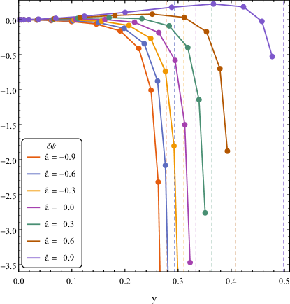
Figure 1: Numerical results for $\delta\psi$ for various values of the spin $a$. The vertical dashed lines show the location of the lightring for that value of the spin, where $\delta\psi$ diverges.

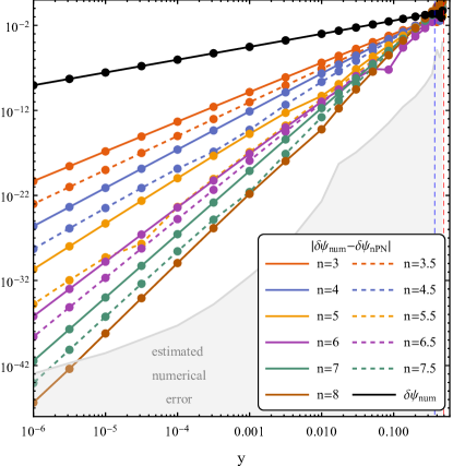
Figure 2: Comparison of the numerical and PN results for $\delta\psi$ in the weak field regime for $\hat{a}=0.9$. The plotted lines show the residual after subtracting the $n$th order PN approximation. The slopes of each line is compatible with an $(n+1/2)th$ order residual, as one would expect. The blue and red vertical dashed lines show the location of the ISCO and the lightring respectively. The shade region gives an estimate on the numerical error in the calculation of $\delta\psi_{\mathrm{num}}$

Figure 3: Comparison of the numerical and PN results for $\delta\psi$ in the strong field regime for $\hat{a}=0.9$. Above $y\approx 0.23$ the PN residuals no longer consistently improve with higher PN order, demonstrating the asymptotic nature of the PN expansion. The relatively good performance of the $6PN$ approximant seems mostly coincidental due to a zero crossing. The blue and red vertical dashed lines show the location of the ISCO and the lightring respectively.

Method III obtains high accuracy numerical results for $\delta\psi$ without any post-Newtonian assumptions. Fig. 1 shows the results for a variety of spins. One obvious feature is that as the (unstable) circular orbits approach the lightring $\delta\psi$ diverges. This behaviour is well-known in the analogous case of the redshift invariant Barack and Sago (2011); Akcay et al. (2012); Bini et al. (2015), and was studied in the case of $\delta\psi$ around Schwarzschild in Bini and Damour (2014d), which concluded that the light-ring divergence of $\delta\psi$ is proportional to $E^{2}$, where $E$ is the orbital energy. The data here is also compatible with a divergence $\propto E^{2}$. The full numerical results are available from the black hole perturbation toolkit website BHP .

Fig. 2 shows a comparison of the numerical results with the obtained PN results in the weak field regime. Shown are the residuals after subtracting successive orders in the PN expansion. We see a consistent improvement in the weak field, providing a strong verification of both the analytical PN results and the numerical results.

Fig. 3 shows the same plot but with a focus on the strong field regime. Here the picture is very different. Around $y\approx 0.24$ we observe a locus where all PN approximants do about equally well (with the 6 and 6.5 PN terms as notable exceptions). Above this there is no noticeable improvement from going to higher PN orders.

V Discussion and outlook

In this paper we have, for the first time, calculated the GSF corrections to the spin precession invariant along circular equatorial geodesic orbits in a perturbed Kerr spacetime, generalizing previous results limited to the case of a perturbed Schwarzschild spacetime. This calculation has been done with a variety of methods and techniques providing ample cross-validation.

Comparison with existing PN results using the first law of binary mechanics Blanchet et al. (2013), provides a strong validation of the used radiation gauge GSF techniques employed here, while also validating the previous PN results.

Cross validation between the different GSF calculations, which vary in the level of rigor in their derivation, validates some of the underlying assumptions. In particular, a subtle importance is the agreement we find between the methods despite the differences in harmonic projections. State of the art radiation gauge self-force codes project from spin-weighted spheroidal harmonics to scalar spherical harmonics to meet up with rigorously defined regularization techniques, which has a large negative impact on the computational costs. In this work we have shown agreement between such a projected numerical code, and an unprojected analytical code without needing and additional correction terms. Investigating if such agreements between projections hold in more generic orbital configurations or for gauge dependent quantities (such as the self-force itself) would be of great importance in developing more efficient numerical codes for realistic self-force models.

An important application of the results in this paper will be to inform effective-one-body (EOB) theory Buonanno and Damour (1999); Damour (2001). As shown in Bini and Damour (2014d), the spin precession can be used to determine contributions to the effective-one-body Hamiltonian for spinning black holes relating to the secondary spin. This transcription will be left to future work.

This work, focusing on circular equatorial orbits, is a first step in determining the spin precession around Kerr black holes. The formalism for extending this work to eccentric equatorial orbits has already been laid out Akcay (2017) and should provide a basis for generalizing to generically inclined orbits. This should provide additional avenues of cross-validating difficult GSF calculations and informing EOB.

References

- Abbott et al. (2016a) B. P. Abbott et al. (Virgo, LIGO Scientific), “Observation of Gravitational Waves from a Binary Black Hole Merger,” Phys. Rev. Lett. 116, 061102 (2016a), arXiv:1602.03837 [gr-qc] .
- Abbott et al. (2016b) B. P. Abbott et al. (Virgo, LIGO Scientific), “GW151226: Observation of Gravitational Waves from a 22-Solar-Mass Binary Black Hole Coalescence,” Phys. Rev. Lett. 116, 241103 (2016b), arXiv:1606.04855 [gr-qc] .
- Abbott et al. (2017a) B. P. Abbott et al. (Virgo, LIGO Scientific), “GW170814: A Three-Detector Observation of Gravitational Waves from a Binary Black Hole Coalescence,” Phys. Rev. Lett. 119, 141101 (2017a), arXiv:1709.09660 [gr-qc] .
- Abbott et al. (2017b) B. P. Abbott et al. (Virgo, LIGO Scientific), “GW170817: Observation of Gravitational Waves from a Binary Neutron Star Inspiral,” Phys. Rev. Lett. 119, 161101 (2017b), arXiv:1710.05832 [gr-qc] .
- Klein et al. (2016) Antoine Klein et al., “Science with the space-based interferometer eLISA: Supermassive black hole binaries,” Phys. Rev. D93, 024003 (2016), arXiv:1511.05581 [gr-qc] .
- Caprini et al. (2016) Chiara Caprini et al., “Science with the space-based interferometer eLISA. II: Gravitational waves from cosmological phase transitions,” JCAP 1604, 001 (2016), arXiv:1512.06239 [astro-ph.CO] .
- Tamanini et al. (2016) Nicola Tamanini, Chiara Caprini, Enrico Barausse, Alberto Sesana, Antoine Klein, and Antoine Petiteau, “Science with the space-based interferometer eLISA. III: Probing the expansion of the Universe using gravitational wave standard sirens,” JCAP 1604, 002 (2016), arXiv:1601.07112 [astro-ph.CO] .
- Bartolo et al. (2016) Nicola Bartolo et al., “Science with the space-based interferometer LISA. IV: Probing inflation with gravitational waves,” JCAP 1612, 026 (2016), arXiv:1610.06481 [astro-ph.CO] .
- Babak et al. (2017) Stanislav Babak, Jonathan Gair, Alberto Sesana, Enrico Barausse, Carlos F. Sopuerta, Christopher P. L. Berry, Emanuele Berti, Pau Amaro-Seoane, Antoine Petiteau, and Antoine Klein, “Science with the space-based interferometer LISA. V: Extreme mass-ratio inspirals,” Phys. Rev. D95, 103012 (2017), arXiv:1703.09722 [gr-qc] .
- Barack et al. (2010) Leor Barack, Thibault Damour, and Norichika Sago, “Precession effect of the gravitational self-force in a Schwarzschild spacetime and the effective one-body formalism,” Phys. Rev. D 82, 084036 (2010), arXiv:1008.0935 [gr-qc] .
- van de Meent (2017) Maarten van de Meent, “Self-force corrections to the periapsis advance around a spinning black hole,” Phys. Rev. Lett. 118, 011101 (2017), arXiv:1610.03497 [gr-qc] .
- Detweiler (2008) Steven L. Detweiler, “A Consequence of the gravitational self-force for circular orbits of the Schwarzschild geometry,” Phys. Rev. D 77, 124026 (2008), arXiv:0804.3529 [gr-qc] .
- Barack and Sago (2011) Leor Barack and Norichika Sago, “Beyond the geodesic approximation: conservative effects of the gravitational self-force in eccentric orbits around a Schwarzschild black hole,” Phys. Rev. D 83, 084023 (2011), arXiv:1101.3331 [gr-qc] .
- Sago et al. (2008) Norichika Sago, Leor Barack, and Steven L. Detweiler, “Two approaches for the gravitational self force in black hole spacetime: Comparison of numerical results,” Phys. Rev. D 78, 124024 (2008), arXiv:0810.2530 [gr-qc] .
- Shah et al. (2011) Abhay G. Shah, Tobias S. Keidl, John L. Friedman, Dong-Hoon Kim, and Larry R. Price, “Conservative, gravitational self-force for a particle in circular orbit around a Schwarzschild black hole in a Radiation Gauge,” Phys. Rev. D 83, 064018 (2011), arXiv:1009.4876 [gr-qc] .
- Shah et al. (2012) Abhay G. Shah, John L. Friedman, and Tobias S. Keidl, “EMRI corrections to the angular velocity and redshift factor of a mass in circular orbit about a Kerr black hole,” Phys. Rev. D 86, 084059 (2012), arXiv:1207.5595 [gr-qc] .
- van de Meent and Shah (2015) Maarten van de Meent and Abhay G. Shah, “Metric perturbations produced by eccentric equatorial orbits around a Kerr black hole,” Phys. Rev. D 92, 064025 (2015), arXiv:1506.04755 [gr-qc] .
- Kavanagh et al. (2016) Chris Kavanagh, Adrian C. Ottewill, and Barry Wardell, “Analytical high-order post-Newtonian expansions for spinning extreme mass ratio binaries,” Phys. Rev. D 93, 124038 (2016), arXiv:1601.03394 [gr-qc] .
- Kavanagh et al. (2015) Chris Kavanagh, Adrian C. Ottewill, and Barry Wardell, “Analytical high-order post-Newtonian expansions for extreme mass ratio binaries,” Phys. Rev. D 92, 084025 (2015), arXiv:1503.02334 [gr-qc] .
- Bini et al. (2016a) Donato Bini, Thibault Damour, and Andrea Geralico, “High post-Newtonian order gravitational self-force analytical results for eccentric equatorial orbits around a Kerr black hole,” Phys. Rev. D93, 124058 (2016a), arXiv:1602.08282 [gr-qc] .
- Barack and Pound (2018) Leor Barack and Adam Pound, “Self-force and radiation reaction in general relativity,” (2018), arXiv:1805.10385 [gr-qc] .
- Dolan et al. (2014) Sam R. Dolan, Niels Warburton, Abraham I. Harte, Alexandre Le Tiec, Barry Wardell, and Leor Barack, “Gravitational self-torque and spin precession in compact binaries,” Phys. Rev. D89, 064011 (2014), arXiv:1312.0775 [gr-qc] .
- Bini and Damour (2014a) Donato Bini and Thibault Damour, “Two-body gravitational spin-orbit interaction at linear order in the mass ratio,” Phys. Rev. D90, 024039 (2014a), arXiv:1404.2747 [gr-qc] .
- Akcay et al. (2017) Sarp Akcay, David Dempsey, and Sam R. Dolan, “Spin–orbit precession for eccentric black hole binaries at first order in the mass ratio,” Class. Quant. Grav. 34, 084001 (2017), arXiv:1608.04811 [gr-qc] .
- Kavanagh et al. (2017) Chris Kavanagh, Donato Bini, Thibault Damour, Seth Hopper, Adrian C. Ottewill, and Barry Wardell, “Spin-orbit precession along eccentric orbits for extreme mass ratio black hole binaries and its effective-one-body transcription,” Phys. Rev. D96, 064012 (2017), arXiv:1706.00459 [gr-qc] .
- Akcay (2017) Sarp Akcay, “Self-force correction to geodetic spin precession in Kerr spacetime,” Phys. Rev. D96, 044024 (2017), arXiv:1705.03282 [gr-qc] .
- Bini and Damour (2013) Donato Bini and Thibault Damour, “Analytical determination of the two-body gravitational interaction potential at the fourth post-Newtonian approximation,” Phys. Rev. D87, 121501 (2013), arXiv:1305.4884 [gr-qc] .
- Bini and Damour (2014b) Donato Bini and Thibault Damour, “High-order post-Newtonian contributions to the two-body gravitational interaction potential from analytical gravitational self-force calculations,” Phys. Rev. D89, 064063 (2014b), arXiv:1312.2503 [gr-qc] .
- Bini and Damour (2014c) Donato Bini and Thibault Damour, “Analytic determination of the eight-and-a-half post-Newtonian self-force contributions to the two-body gravitational interaction potential,” Phys. Rev. D 89, 104047 (2014c), arXiv:1403.2366 [gr-qc] .
- Hopper et al. (2016) Seth Hopper, Chris Kavanagh, and Adrian C. Ottewill, “Analytic self-force calculations in the post-Newtonian regime: eccentric orbits on a Schwarzschild background,” Phys. Rev. D93, 044010 (2016), arXiv:1512.01556 [gr-qc] .
- Johnson-McDaniel et al. (2015) Nathan K. Johnson-McDaniel, Abhay G. Shah, and Bernard F. Whiting, “Experimental mathematics meets gravitational self-force,” (2015), arXiv:1503.02638 [gr-qc] .
- Bini and Damour (2015a) Donato Bini and Thibault Damour, “Detweiler’s gauge-invariant redshift variable: Analytic determination of the nine and nine-and-a-half post-Newtonian self-force contributions,” Phys. Rev. D 91, 064050 (2015a), arXiv:1502.02450 [gr-qc] .
- Bini et al. (2016b) Donato Bini, Thibault Damour, and Andrea Geralico, “Confirming and improving post-Newtonian and effective-one-body results from self-force computations along eccentric orbits around a Schwarzschild black hole,” Phys. Rev. D 93, 064023 (2016b), arXiv:1511.04533 [gr-qc] .
- Bini et al. (2016c) Donato Bini, Thibault Damour, and Andrea Geralico, “New gravitational self-force analytical results for eccentric orbits around a Schwarzschild black hole,” Phys. Rev. D 93, 104017 (2016c), arXiv:1601.02988 [gr-qc] .
- Bini et al. (2018a) Donato Bini, Thibault Damour, Andrea Geralico, and Chris Kavanagh, “Detweiler’s redshift invariant for spinning particles along circular orbits on a Schwarzschild background,” Phys. Rev. D97, 104022 (2018a), arXiv:1801.09616 [gr-qc] .
- Shah et al. (2014) Abhay G Shah, John L Friedman, and Bernard F Whiting, “Finding high-order analytic post-Newtonian parameters from a high-precision numerical self-force calculation,” Phys. Rev. D 89, 064042 (2014), arXiv:1312.1952 [gr-qc] .
- Bini et al. (2015) Donato Bini, Thibault Damour, and Andrea Geralico, “Spin-dependent two-body interactions from gravitational self-force computations,” Phys. Rev. D92, 124058 (2015), [Erratum: Phys. Rev.D93,no.10,109902(2016)], arXiv:1510.06230 [gr-qc] .
- Bini and Damour (2015b) Donato Bini and Thibault Damour, “Analytic determination of high-order post-Newtonian self-force contributions to gravitational spin precession,” Phys. Rev. D 91, 064064 (2015b), arXiv:1503.01272 [gr-qc] .
- Shah and Pound (2015) Abhay G. Shah and Adam Pound, “Linear-in-mass-ratio contribution to spin precession and tidal invariants in Schwarzschild spacetime at very high post-Newtonian order,” Phys. Rev. D91, 124022 (2015), arXiv:1503.02414 [gr-qc] .
- Bini et al. (2018b) Donato Bini, Thibault Damour, and Andrea Geralico, “Spin-orbit precession along eccentric orbits: improving the knowledge of self-force corrections and of their effective-one-body counterparts,” Phys. Rev. D97, 104046 (2018b), arXiv:1801.03704 [gr-qc] .
- Dolan et al. (2015) Sam R. Dolan, Patrick Nolan, Adrian C. Ottewill, Niels Warburton, and Barry Wardell, “Tidal invariants for compact binaries on quasicircular orbits,” Phys. Rev. D 91, 023009 (2015), arXiv:1406.4890 [gr-qc] .
- Bini and Damour (2014d) Donato Bini and Thibault Damour, “Gravitational self-force corrections to two-body tidal interactions and the effective one-body formalism,” Phys. Rev. D 90, 124037 (2014d), arXiv:1409.6933 [gr-qc] .
- Bini and Geralico (2018a) Donato Bini and Andrea Geralico, “Gravitational self-force corrections to tidal invariants for particles on eccentric orbits in a Schwarzschild spacetime,” (2018a), arXiv:1806.06635 [gr-qc] .
- Bini and Geralico (2018b) Donato Bini and Andrea Geralico, “Gravitational self-force corrections to tidal invariants for particles on circular orbits in a Kerr spacetime,” (2018b), arXiv:1806.08765 [gr-qc] .
- Nolan et al. (2015) Patrick Nolan, Chris Kavanagh, Sam R Dolan, Adrian C Ottewill, Niels Warburton, et al., “Octupolar invariants for compact binaries on quasi-circular orbits,” (2015), arXiv:1505.04447 [gr-qc] .
- Cohen and Kegeles (1974) J.M. Cohen and L.S. Kegeles, “Electromagnetic fields in curved spaces - a constructive procedure,” Phys. Rev. D 10, 1070–1084 (1974).
- Chrzanowski (1975) P.L. Chrzanowski, “Vector Potential and Metric Perturbations of a Rotating Black Hole,” Phys. Rev. D 11, 2042–2062 (1975).
- Kegeles and Cohen (1979) L.S. Kegeles and J.M. Cohen, “Constructive procedure for perturbations of space-times,” Phys. Rev. D 19, 1641–1664 (1979).
- Wald (1978) Robert M. Wald, “Construction of Solutions of Gravitational, Electromagnetic, Or Other Perturbation Equations from Solutions of Decoupled Equations,” Phys. Rev. Lett. 41, 203–206 (1978).
- Lousto and Whiting (2002) Carlos O. Lousto and Bernard F. Whiting, “Reconstruction of black hole metric perturbations from Weyl curvature,” Phys. Rev. D 66, 024026 (2002), arXiv:gr-qc/0203061 .
- Ori (2003) Amos Ori, “Reconstruction of inhomogeneous metric perturbations and electromagnetic four potential in Kerr space-time,” Phys. Rev. D 67, 124010 (2003), arXiv:gr-qc/0207045 .
- Keidl et al. (2010) Tobias S. Keidl, Abhay G. Shah, John L. Friedman, Dong-Hoon Kim, and Larry R. Price, “Gravitational Self-force in a Radiation Gauge,” Phys. Rev. D 82, 124012 (2010), arXiv:1004.2276 [gr-qc] .
- Barack and Ori (2001) Leor Barack and Amos Ori, “Gravitational selfforce and gauge transformations,” Phys. Rev. D 64, 124003 (2001), arXiv:gr-qc/0107056 .
- Pound et al. (2014) Adam Pound, Cesar Merlin, and Leor Barack, “Gravitational self-force from radiation-gauge metric perturbations,” Phys. Rev. D 89, 024009 (2014), arXiv:1310.1513 [gr-qc] .
- Keidl et al. (2007) Tobias S. Keidl, John L. Friedman, and Alan G. Wiseman, “On finding fields and self-force in a gauge appropriate to separable wave equations,” Phys. Rev. D 75, 124009 (2007), arXiv:gr-qc/0611072 .
- Mano and Takasugi (1997) Shuhei Mano and Eiichi Takasugi, “Analytic solutions of the Teukolsky equation and their properties,” 97, 213–232 (1997), arXiv:gr-qc/9611014 .
- Mano et al. (1996) Shuhei Mano, Hisao Suzuki, and Eiichi Takasugi, “Analytic solutions of the Teukolsky equation and their low frequency expansions,” 95, 1079–1096 (1996), arXiv:gr-qc/9603020 .
- Fujita and Tagoshi (2004) Ryuichi Fujita and Hideyuki Tagoshi, “New numerical methods to evaluate homogeneous solutions of the Teukolsky equation,” 112, 415–450 (2004), arXiv:gr-qc/0410018 .
- Fujita et al. (2009) Ryuichi Fujita, Wataru Hikida, and Hideyuki Tagoshi, “An Efficient Numerical Method for Computing Gravitational Waves Induced by a Particle Moving on Eccentric Inclined Orbits around a Kerr Black Hole,” 121, 843–874 (2009), arXiv:0904.3810 [gr-qc] .
- Throwe (2010) William Throwe, “High precision calculation of generic extreme mass ratio inspirals,” (2010), MIT bachelor’s thesis.
- Detweiler and Whiting (2003) Steven L. Detweiler and Bernard F. Whiting, “Selfforce via a Green’s function decomposition,” Phys. Rev. D 67, 024025 (2003), arXiv:gr-qc/0202086 .
- Barack et al. (2002) Leor Barack, Yasushi Mino, Hiroyuki Nakano, Amos Ori, and Misao Sasaki, “Calculating the gravitational selfforce in Schwarzschild space-time,” Phys. Rev. Lett. 88, 091101 (2002), arXiv:gr-qc/0111001 [gr-qc] .
- Heffernan et al. (2014) Anna Heffernan, Adrian Ottewill, and Barry Wardell, “High-order expansions of the Detweiler-Whiting singular field in Kerr spacetime,” Phys. Rev. D 89, 024030 (2014), arXiv:1211.6446 [gr-qc] .
- (64) Adam Pound, Maarten van de Meent, and Abhay G Shah, “Quasi-invariants from radiation gauge self-force calculations,” (unpublished).
- Merlin et al. (2016) Cesar Merlin, Amos Ori, Leor Barack, Adam Pound, and Maarten van de Meent, “Completion of metric reconstruction for a particle orbiting a Kerr black hole,” Phys. Rev. D 94, 104066 (2016), arXiv:1609.01227 [gr-qc] .
- van De Meent (2017) Maarten van De Meent, “The mass and angular momentum of reconstructed metric perturbations,” Class. Quant. Grav. 34, 124003 (2017), arXiv:1702.00969 [gr-qc] .
- Blanchet et al. (2013) Luc Blanchet, Alessandra Buonanno, and Alexandre Le Tiec, “First law of mechanics for black hole binaries with spins,” Phys. Rev. D 87, 024030 (2013), arXiv:1211.1060 [gr-qc] .
- Levi and Steinhoff (2016) Michele Levi and Jan Steinhoff, “Next-to-next-to-leading order gravitational spin-orbit coupling via the effective field theory for spinning objects in the post-Newtonian scheme,” JCAP 1601, 011 (2016), arXiv:1506.05056 [gr-qc] .
- Iyer and Vishveshwara (1993) Bala R. Iyer and C. V. Vishveshwara, “The Frenet-Serret description of gyroscopic precession,” Phys. Rev. D48, 5706–5720 (1993), arXiv:gr-qc/9310019 [gr-qc] .
- Akcay et al. (2012) Sarp Akcay, Leor Barack, Thibault Damour, and Norichika Sago, “Gravitational self-force and the effective-one-body formalism between the innermost stable circular orbit and the light ring,” Phys. Rev. D 86, 104041 (2012), arXiv:1209.0964 [gr-qc] .
- (71) “Black Hole Perturbation Toolkit,” bhptoolkit.org.
- Buonanno and Damour (1999) A. Buonanno and T. Damour, “Effective one-body approach to general relativistic two-body dynamics,” Phys. Rev. D 59, 084006 (1999), arXiv:gr-qc/9811091 .
- Damour (2001) Thibault Damour, “Coalescence of two spinning black holes: an effective one-body approach,” Phys. Rev. D64, 124013 (2001), arXiv:gr-qc/0103018 [gr-qc] .