Lattice Boltzmann model with self-tuning equation of state for multiphase flows

Abstract

A novel lattice Boltzmann (LB) model for multiphase flows is developed that complies with the thermodynamic foundations of kinetic theory. By directly devising the collision term for LB equation at the discrete level, a self-tuning equation of state is achieved, which can be interpreted as the incorporation of short-range molecular interaction. A pairwise interaction force is introduced to mimic the long-range molecular interaction, which is responsible for interfacial dynamics. The derived pressure tensor is naturally consistent with thermodynamic theory, and surface tension and interface thickness can be independently prescribed.

The lattice Boltzmann (LB) method firstly introduced in 1988 McNamara and Zanetti (1988) uses a set of distribution functions with discrete velocities to depict the complex fluid flows. Due to its kinetic nature, the LB method shows potential for considering microscopic and mesoscopic interactions. It is therefore believed that this method is particularly suitable for multiphase flows, which are complex at the macroscopic level but are much simpler from the microscopic viewpoint. The applications of LB method in multiphase flows emerged in the early 1990s Gunstensen et al. (1991) and have significantly increased in the past decade Li et al. (2016).

Although various LB models for multiphase flows exist Shan and Chen (1993); Swift et al. (1995); He et al. (1998), criticisms have been raised for a long time Luo (1998); He and Doolen (2002). In the pseudopotential LB model Shan and Chen (1993, 1994), a pairwise interaction force is used to mimic the microscopic interaction, which can recover nonideal-gas effects and interfacial dynamics at the same time. However, such simultaneous recoveries make this model suffer from thermodynamic inconsistency, though significant progress has been made in approximating the coexistence densities close to the thermodynamic results Sbragaglia et al. (2007); Li et al. (2012); Khajepor et al. (2015). In the free-energy LB model Swift et al. (1995, 1996), the thermodynamically consistent pressure tensor is directly incorporated to produce the dynamics of multiphase flows. Thus, the annoying evaluations of (high-order) derivatives are unavoidable, though improvements have been made to remedy the violation of Galilean invariance in this model Holdych et al. (1998); Inamuro et al. (2000); Kalarakis et al. (2002, 2003). Different from the pseudopotential and free-energy models, the multiphase LB model has also been developed from kinetic theory via systematic discretization procedures He et al. (1998); He and Doolen (2002). Complicated equivalent force terms exist in this model and severe numerical instability is encountered. Improved models were formulated He et al. (1999); Lee and Lin (2005) at the price of sacrificing the underlying physics and computational simplicity.

In this work, we develop a novel LB model for multiphase flows complying with the thermodynamic foundations of kinetic theory analyzed by He and Doolen He and Doolen (2002). The underlying molecular interaction responsible for multiphase flows is divided into the short-range and long-range parts, which are incorporated by constructing an LB model with self-tuning equation of state (EOS) and introducing a pairwise interaction force, respectively. The present LB model has the advantages of the popular pseudopotential and free-energy LB models and is free of the aforementioned drawbacks.

With the presence of a discrete force term $F_{v,i}$, the LB equation for the density distribution function $f_{i}$ can be generally expressed as McCracken and Abraham (2005)

$$f_{i}(\mathbf{x}+\mathbf{e}_{i}\delta_{t},t+\delta_{t})=f_{i}+\delta_{t}F_{v,i}-{\it\Lambda}_{ik}\big{(}f_{k}-f_{k}^{\text{eq}}+\tfrac{\delta_{t}}{2}F_{v,k}\big{)},$$ (1)

where $\mathbf{e}_{i}$ is the discrete velocity, ${\it\Lambda}_{ik}$ is the collision matrix in discrete velocity space, and the right-hand side (RHS), termed the collision process, is computed at position $\mathbf{x}$ and time $t$. Owing to the explicit physical significance of the moments of distribution function, it is more convenient to construct the collision term in moment space than in discrete velocity space. Orthogonal moments without weights are adopted Lallemand and Luo (2000), and the RHS of Eq. (1) is transformed into moment space

$$\bar{\mathbf{m}}=\mathbf{m}+\delta_{t}\mathbf{F}_{m}-\mathbf{S}\big{(}\mathbf{m}-\mathbf{m}^{\text{eq}}+\tfrac{\delta_{t}}{2}\mathbf{F}_{m}\big{)},$$ (2)

where $\mathbf{m}=\mathbf{M}(f_{i})^{\text{T}}$ is the rescaled moment with $\mathbf{M}$ being the dimensionless transformation matrix Lallemand and Luo (2000), and $\bar{\mathbf{m}}$ denotes the post-collision moment. For the sake of simplicity, the two-dimensional nine-velocity (D2Q9) lattice is considered here Qian et al. (1992), and the extension to three-dimensional lattice is straightforward though tedious. The equilibrium moment function $\mathbf{m}^{\text{eq}}=\mathbf{M}(f_{i}^{\text{eq}})^{\text{T}}$ is devised as

$$\begin{split}\mathbf{m}^{\text{eq}}=\big{[}\rho,\,2\alpha_{1}\rho+2\beta_{1}\eta+3\rho|\hat{\mathbf{u}}|^{2},\,\alpha_{2}\rho+\beta_{2}\eta-3\rho\times\enskip\quad&\\ |\hat{\mathbf{u}}|^{2}+9\rho\hat{u}_{x}^{2}\hat{u}_{y}^{2},\,\rho\hat{u}_{x},\,-\rho\hat{u}_{x}+3\rho\hat{u}_{x}\hat{u}_{y}^{2},\,\rho\hat{u}_{y},\quad&\\ -\rho\hat{u}_{y}+3\rho\hat{u}_{y}\hat{u}_{x}^{2},\,\rho(\hat{u}_{x}^{2}-\hat{u}_{y}^{2}),\,\rho\hat{u}_{x}\hat{u}_{y}\big{]}^{\text{T}}&,\end{split}$$ (3)

where $\hat{\mathbf{u}}=\mathbf{u}/c$ with lattice speed $c=\delta_{x}/\delta_{t}$, $\eta$ is introduced to achieve the self-tuning EOS, $\alpha_{1,2}$ and $\beta_{1,2}$ are coefficients that will be determined later. The corresponding discrete force term in moment space $\mathbf{F}_{m}=\mathbf{M}(F_{v,i})^{\text{T}}$ is set as follows

$$\begin{split}\mathbf{F}_{m}=\big{\{}0,\;6\hat{\mathbf{F}}\cdot\hat{\mathbf{u}},\,-6\hat{\mathbf{F}}\cdot\hat{\mathbf{u}}+9[\hat{\mathbf{F}}\hat{\mathbf{u}}\hat{\mathbf{u}}\hat{\mathbf{u}}]_{xxyy},\,\hat{F}_{x},\qquad\quad&\\ -\hat{F}_{x}+3[\hat{\mathbf{F}}\hat{\mathbf{u}}\hat{\mathbf{u}}]_{xyy},\,\hat{F}_{y},\,-\hat{F}_{y}+3[\hat{\mathbf{F}}\hat{\mathbf{u}}\hat{\mathbf{u}}]_{xxy},\quad&\\ 2(\hat{F}_{x}\hat{u}_{x}-\hat{F}_{y}\hat{u}_{y}),\,\hat{F}_{x}\hat{u}_{y}+\hat{F}_{y}\hat{u}_{x}\big{\}}^{\text{T}}&,\end{split}$$ (4)

where $\hat{\mathbf{F}}=\mathbf{F}/c$, $[\,\bullet\,]$ denotes permutation and the subscripts denote tensor indices. In Eqs. (3) and (4), the high-order terms of velocity correspond to the third- and fourth-order Hermite terms in $f_{i}^{\text{eq}}$ and $F_{v,i}$, whose effects will be discussed later. The macroscopic density $\rho$ and velocity $\mathbf{u}$ are defined as

$$\rho=\sum\nolimits_{i}f_{i},\quad\rho\mathbf{u}=\sum\nolimits_{i}\mathbf{e}_{i}f_{i}+\tfrac{\delta_{t}}{2}\mathbf{F}.$$ (5)

Once the equilibrium distribution function in LB equation is changed to achieve self-tuning EOS, it has been recognized previously that Newtonian viscous stress cannot be recovered correctly, and Galilean invariance will be lost Swift et al. (1996); Dellar (2002). From the Enskog equation for dense gases in kinetic theory, we note that an extra velocity-dependent term emerges in the collision term Chapman and Cowling (1970); Luo (1998); He and Doolen (2002). Inspired by this fact, some velocity-dependent non-diagonal elements are introduced in the collision matrix $\mathbf{S}$

$$\mathbf{S}=\!\begin{bmatrix}s_{0}&0&0&0&0&0&0&0&0\\ 0&s_{e}&ks_{\varepsilon}\omega_{e}&0&h\hat{u}_{x}s_{q}\omega_{e}&0&h\hat{u}_{y}s_{q}\omega_{e}&0&0\\ 0&0&s_{\varepsilon}&0&0&0&0&0&0\\ 0&0&0&s_{j}&0&0&0&0&0\\ 0&0&0&0&s_{q}&0&0&0&0\\ 0&0&0&0&0&s_{j}&0&0&0\\ 0&0&0&0&0&0&s_{q}&0&0\\ 0&0&0&0&2b\hat{u}_{x}s_{q}\omega_{p}&0&-2b\hat{u}_{y}s_{q}\omega_{p}&s_{p}&0\\ 0&0&0&0&b\hat{u}_{y}s_{q}\omega_{p}&0&b\hat{u}_{x}s_{q}\omega_{p}&0&s_{p}\\ \end{bmatrix},$$ (6)

where $\omega_{e,p}=s_{e,p}/2-1$, and $k$, $h$ and $b$ are coefficients. Note that this improved collision matrix is still invertible. Through the Chapman-Enskog (CE) analysis and to recover the correct Newtonian viscous stress (see Supplemental Material for details Sup ), the coefficients in $\mathbf{m}^{\text{eq}}$ and $\mathbf{S}$ should satisfy

$$\begin{array}[]{c}\alpha_{2}=-\tfrac{2\alpha_{1}+\varpi+1}{1-\varpi},\quad\beta_{2}=-\tfrac{2\beta_{1}}{1-\varpi},\\[4.30554pt] k=1-\varpi,\quad h=\tfrac{6\varpi(1-\varpi)}{1-3\varpi},\quad b=\tfrac{1-\varpi}{1-3\varpi},\end{array}$$ (7)

where $\varpi$ is related to the bulk viscosity. The recovered macroscopic equation at the Navier-Stokes level is

$$\begin{cases}\partial_{t}\rho+\nabla\cdot(\rho\mathbf{u})=0,\\ \partial_{t}(\rho\mathbf{u})+\nabla\cdot(\rho\mathbf{uu})=-\nabla p_{\text{\tiny LBE}}+\mathbf{F}+\nabla\cdot\mathbf{\Pi}+O(M\mspace{-3.0mu}a^{3}),\end{cases}$$ (8)

where $p_{\text{\tiny LBE}}$ is the recovered EOS, $\mathbf{\Pi}=\rho\nu[\nabla\mathbf{u}+\mathbf{u}\nabla-(\nabla\cdot\mathbf{u})\mathbf{I}]+\rho\varsigma(\nabla\cdot\mathbf{u})\mathbf{I}$ is the recovered Newtonian viscous stress, and $M\mspace{-3.0mu}a$ denotes the Mach number. Here, the EOS $p_{\text{\tiny LBE}}$, the kinematic viscosity $\nu$ and the bulk viscosity $\varsigma$ are expressed as

$$\begin{array}[]{c}p_{\text{\tiny LBE}}=c_{s}^{2}[(2+\alpha_{1})\rho+\beta_{1}\eta],\\[4.30554pt] \nu=c_{s}^{2}\big{(}s_{p}^{-1}-\tfrac{1}{2}\big{)}\delta_{t},\quad\varsigma=\varpi c_{s}^{2}\big{(}s_{e}^{-1}-\tfrac{1}{2}\big{)}\delta_{t},\end{array}$$ (9)

with lattice sound speed $c_{s}=c/\sqrt{3}$. Obviously, $p_{\text{\tiny LBE}}$ can be arbitrarily tuned via the built-in $\eta$. Before proceeding further, some discussion on the present LB model with self-tuning EOS is useful. For the coefficients $\alpha_{1,2}$ and $\beta_{1,2}$, $\alpha_{1}=-1$ and $\beta_{1}=1$ are set as ordinary, and one has $\alpha_{2}=1$. Therefore, $\mathbf{m}^{\text{eq}}$ given by Eq. (3) can be decomposed into the ordinary one derived from the Hermite expansion of the Maxwell-Boltzmann distribution and the extra one related to $\eta$. The coefficient $\varpi$ plays an important role here. When $\varpi=1$, one has $\beta_{2}\rightarrow\infty$, $k=0$, $h=0$, and $b=0$. Thus, $\eta$ should be set to $0$ to avoid singularity, implying that the present model degenerates into the classical LB model with ideal-gas EOS. When $\varpi=1/3$, one has $\beta_{2}=-3$, $k=2/3$, $h\rightarrow\infty$, and $b\rightarrow\infty$. Thus, the velocity-dependent terms in $\mathbf{S}$ should be removed to avoid singularity, which means that Newtonian viscous stress cannot be recovered and Galilean invariance is lost. Compared with previous LB models derived from the Enskog equation via systematic discretization procedures Luo (1998); He et al. (1998); He and Doolen (2002), the present model is directly constructed at the discrete level in moment space and thus is free of complicated derivative terms, which trigger numerical instability and restrict real applications of previous models He et al. (1999); Lee and Lin (2005).

In the macroscopic equation recovered at the Navier-Stokes level [Eq. (8)], some cubic terms of velocity exist, which are usually ignored under the low Mach number condition in LB method. By retaining the high-order terms of velocity in $\mathbf{m}^{\text{eq}}$ and $\mathbf{F}_{m}$ [Eqs. (3) and (4)], the additional cubic terms can be partially eliminated Dellar (2014). To eliminate the remaining cubic terms, the collision process described by Eq. (2) can be improved as

$$\begin{split}\bar{\mathbf{m}}=\mathbf{m}+\delta_{t}\mathbf{F}_{m}-\mathbf{S}\left(\mathbf{m}-\mathbf{m}^{\text{eq}}+\tfrac{\delta_{t}}{2}\mathbf{F}_{m}\right)&\\ -\mathbf{R}\left(\mathbf{I}-\tfrac{\mathbf{S}}{2}\right)\left(\mathbf{m}-\mathbf{m}^{\text{eq}}+\tfrac{\delta_{t}}{2}\mathbf{F}_{m}\right)&\\ -\delta_{x}\mathbf{T}\cdot\nabla\rho-\tfrac{\delta_{x}}{c^{2}}\mathbf{X}\cdot\nabla p_{\text{\tiny LBE}}&,\end{split}$$ (10)

where $\mathbf{R}$, $\mathbf{T}$ and $\mathbf{X}$ are $9\times 9$, $9\times 2$ and $9\times 2$ matrices of order $M\mspace{-3.0mu}a^{2}$, $M\mspace{-3.0mu}a^{3}$ and $M\mspace{-3.0mu}a^{3}$, respectively, and thus the corresponding terms have negligible effects on the numerical stability. These correction matrices are set in the following forms Huang et al. (2018)

$$\mathbf{R}=\begin{bmatrix}0&0&0&0&0&0&0&0&0\\[-1.72218pt] 0&R_{11}&0&0&0&0&0&R_{17}&R_{18}\\[-1.72218pt] 0&0&0&0&0&0&0&0&0\\[-1.72218pt] 0&0&0&0&0&0&0&0&0\\[-1.72218pt] 0&0&0&0&0&0&0&0&0\\[-1.72218pt] 0&0&0&0&0&0&0&0&0\\[-1.72218pt] 0&0&0&0&0&0&0&0&0\\[-1.72218pt] 0&R_{71}&0&0&0&0&0&R_{77}&R_{78}\\[-1.72218pt] 0&R_{81}&0&0&0&0&0&R_{87}&R_{88}\\ \end{bmatrix},$$ (11a)

$$\mathbf{T}=(\mathbf{0},\;\mathbf{T}_{1},\;\mathbf{0},\;\mathbf{0},\;\mathbf{0},\;\mathbf{0},\;\mathbf{0},\;\mathbf{T}_{7},\;\mathbf{T}_{8})^{\text{T}},$$ (11b)

$$\mathbf{X}=(\mathbf{0},\;\mathbf{X}_{1},\;\mathbf{0},\;\mathbf{0},\;\mathbf{0},\;\mathbf{0},\;\mathbf{0},\;\mathbf{X}_{7},\;\mathbf{X}_{8})^{\text{T}}.$$ (11c)

Through the CE analysis, the nonzero elements in Eq. (11) can be uniquely and locally determined, and the truncated term in Eq. (8) is improved from $O(M\mspace{-3.0mu}a^{3})$ to $O(M\mspace{-3.0mu}a^{5})$ (see Supplemental Material for details Sup ).

As analyzed by He and Doolen He and Doolen (2002), a thermodynamically consistent kinetic model for multiphase flows can be established by combining Enskog theory for dense gases and mean-field theory for long-range molecular interaction. In the Enskog equation, short-range molecular interaction is considered by the collision term, and consequently nonideal-gas EOS is recovered Chapman and Cowling (1970). From this viewpoint, the present LB model with self-tuning EOS can be interpreted as the incorporation of short-range molecular interaction, and thus the long-range molecular interaction remains to be included to construct a valid model for multiphase flows. Following the idea of the pseudopotential LB model Shan and Chen (1993, 1994), a pairwise interaction force is introduced to mimic the long-range molecular interaction. Here, nearest-neighbor interaction is considered, and the interaction force is given as

$$\mathbf{F}(\mathbf{x})=G^{2}\rho(\mathbf{x})\sum\nolimits_{i}\omega(|\mathbf{e}_{i}\delta_{t}|^{2})\rho(\mathbf{x}+\mathbf{e}_{i}\delta_{t})\mathbf{e}_{i}\delta_{t},$$ (12)

where $G^{2}$ is used to control the interaction strength, and the weights $\omega(\delta_{x}^{2})=1/3$ and $\omega(2\delta_{x}^{2})=1/12$ to maximize the isotropy degree of $\mathbf{F}$. Note that Eq. (12) implies that the long-range molecular interaction is attractive.

The interaction force given by Eq. (12) is incorporated into the LB equation via the discrete force term. Based on our previous analysis Huang and Wu (2016), some $\varepsilon^{3}\text{-order}$ terms will be caused by the discrete lattice effect on the force term, which should be considered for multiphase flows. In order to cancel such effects, a consistent scheme for the $\varepsilon^{3}\text{-order}$ additional term is employed. The collision process described by Eq. (10) is further improved as

$$\begin{split}\bar{\mathbf{m}}=\mathbf{m}+\delta_{t}\mathbf{F}_{m}-\mathbf{S}\left(\mathbf{m}-\mathbf{m}^{\text{eq}}+\tfrac{\delta_{t}}{2}\mathbf{F}_{m}\right)+\mathbf{S}\mathbf{Q}_{m}&\\ -\mathbf{R}\left(\mathbf{I}-\tfrac{\mathbf{S}}{2}\right)\left(\mathbf{m}-\mathbf{m}^{\text{eq}}+\tfrac{\delta_{t}}{2}\mathbf{F}_{m}\right)&\\ -\delta_{x}\mathbf{T}\cdot\nabla\rho-\tfrac{\delta_{x}}{c^{2}}\mathbf{X}\cdot\nabla p_{\text{\tiny LBE}}&,\end{split}$$ (13)

where the discrete additional term $\mathbf{Q}_{m}$ is set as

$$\mathbf{Q}_{m}=\Big{(}0,\,\tfrac{|\tilde{\mathbf{F}}|^{2}}{2},\,-\tfrac{|\tilde{\mathbf{F}}|^{2}}{2},\,0,\,0,\,0,\,0,\,\tfrac{\tilde{F}_{x}^{2}-\tilde{F}_{y}^{2}}{12},\,\tfrac{\tilde{F}_{x}\tilde{F}_{y}}{12}\Big{)}^{\text{T}},$$ (14)

and $\tilde{\mathbf{F}}=\mathbf{F}/(G\rho c)$. In the CE analysis, $\mathbf{F}$ is of order $\varepsilon^{1}$, and thus $\mathbf{Q}_{m}$ is of order $\varepsilon^{2}$. Through the third-order CE analysis, the following macroscopic equation in steady and stationary situation can be recovered (see Supplemental Material for details Sup )

$$\begin{cases}\partial_{t}\rho=0,\\ \partial_{t}(\rho\mathbf{u})=-\nabla p_{\text{\tiny LBE}}+\mathbf{F}+\mathbf{R}_{\text{iso}}+\mathbf{R}_{\text{add}}+\bar{\mathbf{R}}_{\text{iso}}+\bar{\mathbf{R}}_{\text{aniso}},\end{cases}$$ (15)

where $\mathbf{R}_{\text{iso}}=\tfrac{1}{12}\delta_{x}^{2}\nabla\!\cdot\!\nabla\mathbf{F}$ is the isotropic term caused by the discrete lattice effect, $\mathbf{R}_{\text{add}}=-\tfrac{1}{24}c^{2}\nabla\cdot[2\tilde{\mathbf{F}}\tilde{\mathbf{F}}+(\tilde{\mathbf{F}}\cdot\tilde{\mathbf{F}})\mathbf{I}]$ is the additional term introduced by $\mathbf{S}\mathbf{Q}_{m}$ to cancel the effect of $\mathbf{R}_{\text{iso}}$, $\bar{\mathbf{R}}_{\text{iso}}=-\tfrac{1}{6}\delta_{x}^{2}[(k+1)\tau_{e}\tau_{q}-\tau_{p}\tau_{q}]\nabla\!\cdot\!\nabla\nabla\bar{p}$ and $\bar{\mathbf{R}}_{\text{aniso}}=-\tfrac{1}{12}\delta_{x}^{2}(12\tau_{p}\tau_{q}-1)(\partial_{y}^{2}\partial_{x}\bar{p},\,\partial_{x}^{2}\partial_{y}\bar{p})^{\text{T}}$ are the isotropic and anisotropic terms caused by achieving self-tuning EOS, respectively. Here, $\tau_{e,p,q}=s_{e,p,q}^{-1}-1/2$ and $\bar{p}=(3+\beta_{2})c_{s}^{2}\eta$. Note that $\mathbf{R}_{\text{iso}}$, $\mathbf{R}_{\text{add}}$, $\bar{\mathbf{R}}_{\text{iso}}$ and $\bar{\mathbf{R}}_{\text{aniso}}$ are all recovered at the $\varepsilon^{3}\text{-order}$ and thus disappear from the macroscopic equation at the Navier-Stokes level. For multiphase flows, $\bar{\mathbf{R}}_{\text{iso}}$ and $\bar{\mathbf{R}}_{\text{aniso}}$ should be eliminated by setting

$$\tau_{p}\tau_{q}=(k+1)\tau_{e}\tau_{q}=1/12,$$ (16)

and $\mathbf{R}_{\text{iso}}$ and $\mathbf{R}_{\text{add}}$ can be absorbed into the pressure tensor. Therefore, the pressure tensor recovered by the present model is defined as $\nabla\cdot\mathbf{P}=\nabla p_{\text{\tiny LBE}}-\mathbf{F}-\mathbf{R}_{\text{iso}}-\mathbf{R}_{\text{add}}$. By performing Taylor series expansion of the interaction force, the following pressure tensor can be derived (see Supplemental Material for details Sup )

$$\mathbf{P}=\big{(}p_{\text{\tiny EOS}}-\kappa\rho\nabla\!\cdot\!\nabla\rho-\tfrac{\kappa}{2}\nabla\rho\!\cdot\!\nabla\rho\big{)}\mathbf{I}+\kappa\nabla\rho\nabla\rho,$$ (17)

where $\kappa=G^{2}\delta_{x}^{4}/4$ and the EOS is

$$p_{\text{\tiny EOS}}=p_{\text{\tiny LBE}}-\tfrac{G^{2}\delta_{x}^{2}}{2}\rho^{2}.$$ (18)

Obviously, $\mathbf{P}$ given by Eq. (17) is naturally consistent with thermodynamic theory Rowlinson and Widom (1982), where the free energy ${\it\Psi}$ is defined as

$${\it\Psi}=\int_{V}\big{(}\psi_{b}+\tfrac{\kappa}{2}|\nabla\rho|^{2}\big{)}d\mathbf{x}.$$ (19)

Here, $\psi_{b}$ is the bulk free-energy density related to EOS $p_{\text{\tiny EOS}}=\rho\partial_{\rho}\psi_{b}-\psi_{b}$, and $\tfrac{\kappa}{2}|\nabla\rho|^{2}$ is the interfacial free-energy density. Based on Eq. (17), the Maxwell construction can be derived.

In this work, the Carnahan-Starling EOS Carnahan and Starling (1969) is taken as an example

$$p_{\text{\tiny EOS}}=K_{\text{\tiny EOS}}\Big{[}\rho RT\tfrac{1+\vartheta+\vartheta^{2}-\vartheta^{3}}{(1-\vartheta)^{3}}-a\rho^{2}\Big{]},$$ (20)

where $R$ is the gas constant, $T$ is the temperature, $\vartheta=b\rho/4$, $a=0.496388R^{2}T_{c}^{2}/p_{c}$ and $b=0.187295RT_{c}/p_{c}$ with $T_{c}$ and $p_{c}$ denoting the critical temperature and pressure, respectively. The scaling factor $K_{\text{\tiny EOS}}$ Wagner and Pooley (2007) is introduced here to adjust the magnitude of bulk free-energy density $\psi_{b}$. In the Carnahan-Starling EOS, the first and second terms describe the effects of short-range (repulsive) and long-range (attractive) molecular interactions, respectively Carnahan and Starling (1969). Therefore, a consistency between Eqs. (18) and (20) can be established, and then the interaction strength is set as

$$G=K_{\text{\tiny INT}}\sqrt{2K_{\text{\tiny EOS}}a/\delta_{x}^{2}},$$ (21)

where the scaling factor $K_{\text{\tiny INT}}$ is introduced to adjust the interfacial free-energy density $\tfrac{\kappa}{2}|\nabla\rho|^{2}$, and the lattice sound speed is chosen as

$$c_{s}=K_{\text{\tiny INT}}\sqrt{\partial_{\rho}(p_{\text{\tiny EOS}}+K_{\text{\tiny EOS}}a\rho^{2})}\Big{|}_{\rho=\rho_{l}}.$$ (22)

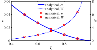
With this configuration, it is known from thermodynamic theory that the surface tension $\sigma$ and interface thickness $W$ satisfy

$$\sigma\propto K_{\text{\tiny EOS}}K_{\text{\tiny INT}},\quad W\propto K_{\text{\tiny INT}},$$ (23)

which have also been numerically validated (see Supplemental Material for details Sup ), and where the proportionality constants can be analytically determined by the pressure tensor. Thus, in real applications of the present LB model, the surface tension and interface thickness can be independently prescribed.

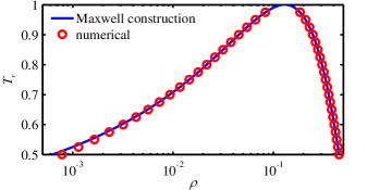
Simulations are performed with $\varpi=1/6$, $a=1$, $b=4$, $R=1$, and $\delta_{x}=1$, and a detailed implementation of the collision process [Eq. (13)] is given in Supplemental Material Sup . The coexistence curve, as a function of reduced temperature $T_{r}$, is firstly computed by simulating a flat interface on a $1024\delta_{x}\times 4\delta_{x}$ domain, as shown in Fig. 1. It can be seen that the numerical result agrees well with the thermodynamic result by Maxwell construction. When $T_{r}<0.6$, there exists slight deviation in the gas branch, which is caused by the spatial discretization error in the interfacial region and can be reduced by increasing the interface thickness. A liquid droplet is then simulated with various $K_{\text{\tiny EOS}}$ and $K_{\text{\tiny INT}}$ on a $1024\delta_{x}\times 1024\delta_{x}$ domain with the droplet diameter being $512\delta_{x}$. Accordingly, the surface tension is calculated via Laplace’s law and the interface thickness is measured from $\rho=0.95\rho_{g}+0.05\rho_{l}$ to $0.05\rho_{g}+0.95\rho_{l}$. Proportionalities described by Eq. (23) can be accurately observed, and the proportionality constants are in good agreement with $\sigma$ and $W$ predicted by $\mathbf{P}$ with $K_{\text{\tiny EOS}}=K_{\text{\tiny INT}}=1$ for flat interface, as shown in Fig. 2.

Figure 1: Coexistence curves obtained by simulation of flat interface and predicted by Maxwell construction.

Figure 2: Proportionality constants in Eq. (23) obtained by simulation of liquid droplet with various $K_{\text{\tiny EOS}}$ and $K_{\text{\tiny INT}}$ and predicted by pressure tensor with $K_{\text{\tiny EOS}}=K_{\text{\tiny INT}}=1$ for flat interface.

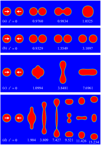
As a dynamic problem, oscillation of an elliptic droplet with the semi-major and minor axes being $96.0\delta_{x}$ and $42.7\delta_{x}$ is simulated on a $512\delta_{x}\times 512\delta_{x}$ domain. Here, $T_{r}=0.6$, $\sigma=0.01$, and $W=10$ are chosen. The oscillation period, numerically measured when the oscillation becomes weak enough, is $18346\delta_{t}$, which agrees well with the analytical solution $18628.0\delta_{t}$ Ana . Head-on collision of equal-sized droplets is further simulated with $T_{r}=0.7$, $\sigma=0.01$, and $W=10$. The computational domain size is $1024\times 1024$, and the droplet diameter is $128\delta_{x}$. The head-on collision outcome is mainly controlled by the Weber number $W\mspace{-3.0mu}e=\rho_{l}U^{2}D/\sigma$ and Reynolds number $R\mspace{-1.0mu}e=UD/\nu$, with $U$ and $D$ denoting the relative velocity and droplet diameter, respectively. All four regimes for head-on collision, experimentally observed by Qian and Law Qian and Law (1997), are successfully reproduced here, as shown in Fig. 3. For $W\mspace{-3.0mu}e=0.01$ and $R\mspace{-1.0mu}e=1$, the droplets approach each other and then merge with small deformation. As $W\mspace{-3.0mu}e$ increases to $0.1$, the droplets bounce back without merging. Here, it is interesting to note that this “bouncing” regime has not been observed in previous simulations by the pseudopotential and free-energy LB models Lycett-Brown et al. (2014); Moqaddam et al. (2016). For $W\mspace{-3.0mu}e=20$ and $R\mspace{-1.0mu}e=100$, merging happens again, accompanied with large deformation in this regime. For $W\mspace{-3.0mu}e=60$ and $R\mspace{-1.0mu}e=200$, the outward motion caused by strong impact splits the merged mass into three parts, with two main droplets separating from both sides and a satellite droplet residing at the center, as shown in Fig. 3(d).

Figure 3: Head-on collision processes of equal-sized droplets at different dimensionless time $t^{\ast}\!=tU/D$ with (a) $W\mspace{-3.0mu}e=0.01$ and $R\mspace{-1.0mu}e=1$, (b) $W\mspace{-3.0mu}e=0.1$ and $R\mspace{-1.0mu}e=1$, (c) $W\mspace{-3.0mu}e=20$ and $R\mspace{-1.0mu}e=100$, and (d) $W\mspace{-3.0mu}e=60$ and $R\mspace{-1.0mu}e=200$.

In summary, we have developed a novel LB model for multiphase flows, which complies with the thermodynamic foundations of kinetic theory and thus is naturally consistent with thermodynamic theory. The underlying short-range and long-range molecular interactions are separately incorporated by constructing an LB model with self-tuning EOS and introducing a pairwise interaction force. The present model combines the advantages of the popular pseudopotential and free-energy LB models. Most computations can be carried out locally, and the surface tension and interface thickness can be independently prescribed in real applications.

See pages 1, of Supplemental_Material.pdf See pages 2, of Supplemental_Material.pdf See pages 3, of Supplemental_Material.pdf See pages 4, of Supplemental_Material.pdf See pages 5, of Supplemental_Material.pdf See pages 6, of Supplemental_Material.pdf See pages 7, of Supplemental_Material.pdf See pages 8, of Supplemental_Material.pdf See pages 9, of Supplemental_Material.pdf See pages 10, of Supplemental_Material.pdf See pages 11, of Supplemental_Material.pdf See pages 12, of Supplemental_Material.pdf See pages 13, of Supplemental_Material.pdf