The assembly history of the Galactic inner halo inferred from $\alpha$-element patterns

Abstract

We explore the origin of the observed decline in [O/Fe] (and [Mg/Fe]) with Galactocentric distance for high-metallicity stars ([Fe/H] $>-1.1$), based on a sample of halo stars selected within the Apache Point Observatory Galactic Evolution Experiment (APOGEE) fourteenth data release (DR14). We also analyse the characteristics of the [$\alpha$/Fe] distributions in the inner-halo regions inferred from two zoom-in Milky Way mass-sized galaxies that are taken as case studies. One of them qualitatively reproduces the observed trend to have higher fraction of $\alpha$-rich star for decreasing galactocentric distance; the other exhibits the opposite trend. We find that stars with [Fe/H] $>-1.1$ located in the range [15 - 30] kpc are consistent with formation in two starbursts, with maxima separated by about $\sim 1$ Gyr. We explore the contributions of stellar populations with different origin to the [$\alpha$/Fe] gradients detected in stars with [Fe/H] $>-1.1$. Our analysis reveals that the simulated halo that best matches the observed chemical trends is characterised by an accretion history involving low to intermediate-mass satellite galaxies with a short and intense burst of star formation, and contributions from a more massive satellite with dynamical masses about $\sim 10^{10}M_{\sun}$, distributing low [$\alpha$/Fe] stars at intermediate radius.

1 Introduction

Observations of the Milky Way (MW) and the haloes of nearby galaxies have revealed spatial sub-structures (Majewski et al., 2003; Belokurov et al., 2006; Morrison et al., 2009; Bonaca et al., 2012; Sesar et al., 2012; Gilbert et al., 2013; Ibata et al., 2014), as well as differences in the kinematical and chemical properties of the stars in the inner region of the Galactic halo with respect to the outer region (Carollo et al., 2007, 2010; Beers et al., 2012; Fernández-Alvar et al., 2015). These results suggest that the stellar populations dominating the inner- and outer-halo regions formed in systems with different star-formation histories. One explanation proposed is that the outer halo was built mainly from mergers of satellite galaxies, whereas the inner halo might have received contributions of stars formed in-situ in the Galaxy (for example stars from a heated disc due to merger events, e.g. Sheffield et al., 2012; Nissen & Schuster, 2010; Schuster et al., 2012)

The formation of the stellar halo has been tackled using dynamical and hydrodynamical simulations (e.g., Bullock et al., 2010; Cooper et al., 2010; Tissera et al., 2013; Pillepich et al., 2015). All of these works predict the formation of the stellar halo mainly from the contribution of satellites with a variety of masses. However, hydrodynamical simulations also reported the possible existence of an in-situ component (Zolotov et al., 2009; Tissera et al., 2012; Cooper et al., 2015). Disc-heated stars are a possible candidate to explain the origin of the in-situ components (as proposed from both numerical simulations as well as observational works, e.g. Tissera et al., 2014; Bonaca et al., 2017), but they might have also formed from gas transported in by gas-rich satellites (Zolotov et al., 2009; Tissera et al., 2013). Harmsen et al. (2017) found that these simulations were able to reproduce global trends of the stellar haloes of nearby galaxies, although most of them predicted more massive stellar haloes than inferred from observations, and larger contributions of in-situ stars compared to the observed estimates.

However, recently observations have shown evidence for the accretion of a relatively massive satellite contributing stars to the inner halo of the Milky Way. Belokurov et al. (2018) observed that the orbits of stars with [Fe/H] $>-1.7$ are strongly radial, in a sausage-like distribution, and, by comparing with N-body simulations, deduced that they come from the merger of a satellite with virial mass M $>10^{10}$ M_⊙, which was called in following works the “Gaia sausage". Using data from the Gaia second data release (DR2), Deason et al. (2018) obtained that stars with very radial orbits (like in the “Gaia sausage") have apocentres which pile up at $r\sim$ 20 kpc, where the spatial break in the halo was measured in numerous previous papers. They conclude that these stars likely come from a satellite with stellar mass at least M $>10^{8}$ M_⊙, or from a group of dwarf satellites accreted at similar times. Helmi et al. (2018) identified stars in retrograde orbits, and they also constrained (from the star-formation rates obtained from similar stars in Fernández-Alvar et al., 2018b) the stellar mass of their progenitor satellite to be $\sim 6\times 10^{8}$ M_⊙ (which they called “Gaia-Enceladus").

From the analysis of globular clusters in the Galactic halo, other evidence was found for relatively massive mergers. Myeong et al. (2018) confirmed that the configuration of a group of globular clusters in action space is compatible with their coming from the “Gaia sausage" merger event. Kruijssen et al. (2018) used the age-metallicity relation in halo clusters, compared with the E-MOSAICS hydrodynamical simulations, to infer that the MW may have undergone mergers with three satellites with stellar masses between $10^{8}$ and $10^{9}$ (the most massive of which they refer to as “Kraken"). Other evidences have been also provided by Lancaster et al. (2018); Haywood et al. (2018); Fernández-Alvar et al. (2018a); Simion et al. (2018); Iorio & Belokurov (2018); Wegg et al. (2018); Mackereth et al. (2018).

An important piece of information is provided by $\alpha$-element abundances (e.g., Zolotov et al., 2009). Using the Aquarius haloes, Tissera et al. (2013) showed that stars in the stellar haloes have different $\alpha$-enrichments that could provide hints on the mass and star-formation history (SFH) of the accreted satellites, as well as the relative contributions of stars formed through different processes. In their simulations, the authors identifed accreted stars (or debris) formed in systems outside the virial radius of the main galaxy progenitor, and later on, in-situ stars, formed within the virial radius. Within the latter population, they also identified the so-called endo-debris stellar populations, formed from gas carried in by accreted satellites, and disc-heated stars, born in-situ in the disc and later, dynamically heated into the halo. Their different origin predicts different chemical and kinematical patterns in the inner regions of the stellar haloes, in particular different $\alpha$-enhancement patterns.

Indeed, a promising path for investigation is consideration of the [$\alpha$/Fe] abundance ratios that have been derived from observations of large numbers of stars in the MW stellar halo (Fernández-Alvar et al., 2015, 2017). The $\alpha$-elements are ejected into the interstellar medium (ISM) on short timescales (Myr), because these elements are produced mainly by massive stars that explode as Type II supernovae (SNeII). In contrast, release of the bulk of Fe occurs on longer timescales (Gyr), because iron is synthesised by binary stars of low and intermediate mass that explode as Type Ia supernovae (SNeIa) . The patterns in the relative abundances [$\alpha$/Fe] vs. [Fe/H]) are well-known to be affected by the star-formation rate and the initial mass function (e.g., see Fig. 1 of Fernández-Alvar et al. (2018b)).

Fernández-Alvar et al. (2017) identified abundance gradients for $\alpha$-elements and other chemical species relative to the iron abundance with distance from the Galactic center, based on an analysis of over 400 stars from the APOGEE twelfth data release (DR12). They found that the nature of these gradients depended on the [Fe/H] range, flattening as [Fe/H] decreases, suggesting a variation of the chemical-enrichment history for stars as a function of distance. The identification of Galactic halo simulations able to reproduce the observed trends can help to unravel the assembly history of our Galaxy.

In this work, we examine the [$\alpha$/Fe] trends with Galactocentric distance observed in the halo of the MW by the APOGEE fourteenth data release (DR14), which has tripled the number of stars with this information available. We compare them with the trends inferred from a set of simulated haloes of MW mass-size galaxies in order to constrain the assembly history that led to the stellar populations in the inner-halo region with the observed chemical compositions.

We employ the set of Aquarius haloes analysed by Tissera et al. (2012, 2013, 2014) and Carollo et al. (2018) that correspond to MW mass-size galaxies to study the chemical enrichment of baryons during Galactic assembly. These authors found that the stellar halo of the MW is characterised by combination of stellar populations with different chemistry, kinematics, ages, and binding energies depending on their origin. We acknowledge the fact that the Aquarius haloes (Scannapieco et al., 2009) are known to over-produce stars at high redshift. However, they comprise a diversity of assembly histories for galaxies of similar virial masses that allow us to explore which assembly history provides the best representation of the observations. Our approach is to use them as case studies to identify the main processes that could explain the origin of the $\alpha$-abundance patterns detected in observations of the MW’s halo.

This paper is organised as follows. In section 2 we describe the main characteristics of the observational and simulated data used in this work. In section 3 we infer the chemical trends from both sets, and analyse their similarities and differences. Finally, in section 4 we summarise our main results and conclusions.

2 Observational and simulated data

2.1 Observations

We make use of the APOGEE fourteenth data release, DR14 (Blanton et al., 2017). This stellar spectra database includes all the APOGEE observations gathered from May 2011 to July 2014 (Eisenstein et al., 2011), and the observations from the first two years of its extension, APOGEE-2. Using a multi-object infrared spectrograph (Wilson et al., 2010) coupled to the 2.5-meter telescope at the Apache Point Observatory (Gunn et al., 2006), high-resolution ($R\sim 22,500$) spectra were obtained with a typical signal-to-noise S/N$\sim 100$. Targets were spread over the main Galactic components, including the halo (Zasowski et al., 2013, 2017). DR14 offers elemental-abundance determinations for $\sim$19 chemical especies determined by the APOGEE Stellar Parameters and Abundances pipeline (ASPCAP; García Pérez et al., 2016).

We reproduce the analysis performed by Fernández-Alvar et al. (2017), now using the more extended sample of APOGEE-2 stars included in DR14. As in their work, we select stars at distances from the Galactic plane, $|h|$, larger then 5 kpc to avoid contamination from thick-disc stars. We consider distances derived by the Brazilian Participation Group (BPG Santiago et al., 2016; Queiroz et al., 2018) from the spectrophotometric stellar atmospheric parameters (effective temperature, $T_{\rm eff}$, and surface gravity, $\log g$) determined in DR14.

We reject objects with less reliable measured parameters, warned by the flags STAR_BAD, GRIDEDGE_BAD, PERSIST_LOW, PERSIST_MED, PERSIST_HIGH, TEFF_BAD, LOGG_BAD,METALS_BAD, ALPHAFE_BAD, CHI2_BAD, SN_BAD, and NO_ASPCAP_RESULT in the catalogue. In addition, we only consider stars with spectra having S/N $>80$, $T_{\rm eff}>4000$ K, and $1.0<\log g<3.5$.

These were the selection criteria chosen by Fernández-Alvar et al. (2017) for analysing the APOGEE DR12, to which we aim to compare our inferred chemical trends. Thus, we would like to maintain the same $T_{\rm eff}$ and $\log g$ selection cuts for consistence. Besides, although improvements in the ASPCAP were performed in DR14 (see Holtzman et al. (2018)), chemical issues have been still detected related to stars at lower $T_{\rm eff}$ and large $\log g$. For instance, Zasowski et al. (2019) revealed a strange high [O/Fe] trend at Solar metallicities in stars with $T_{\rm eff}<3800$ K. And due to the lack of surface gravity estimations from asteroseismology at the time DR14 was released, calibrated $\log g$ values for stars at $\log g>4$ are still not provided in DR14.

We also exclude stars likely belonging to clusters. We do not exclude targets in streams, because substructures will also be considered in the simulation analysis.

Our final sample comprises 1185 stars. The mean uncertainties estimated and their standard deviations, for the stellar parameters chemical abundances and distances in this stellar sample are the following: $\sigma(T_{\rm eff})=83\pm 17$ K, $\sigma(\log g)=0.09\pm 0.02$, $\sigma($[O/Fe]$)=0.07\pm 0.04$, $\sigma($[Mg/Fe]$)=0.05\pm 0.02$, and $\sigma(d_{\rm sun})/d_{\rm sun}=12\pm 3\%$.

2.2 Simulations

We analysed six Milky-Way mass-sized haloes from the Aquarius project (Scannapieco et al., 2009). The initial conditions of the Aquarius haloes are consistent with a $\Lambda$CDM model with $\Omega_{m}=0.25$, $\Omega_{\Lambda}=0.75$, $\sigma_{8}=0.9$, $n_{S}=1$, and $H_{0}=100h$ km $\rm s^{-1}$ Mp$\rm c^{-1}$ with $h=0.73$. Dark matter particles have masses on the order of $\sim 10^{6}M_{\odot}h^{-1}$; initially the particles have masses of $\sim 2\times 10^{5}M_{\odot}h^{-1}$. The analysed haloes correspond to level-5 resolution. The analysed haloes are Aq-C-5 and Aq-D-5. Hereafter, we will use them Aq-C and Aq-D for simplicity.

The simulations were performed using a modified version of GADGET-3 (Scannapieco et al., 2005, 2006) that includes the physics of the baryons, chemical evolution, and galactic mass-loaded outflows triggered by SNe explosions. The chemical model follows the enrichment from both SNeII and SNeIa.

The galactic systems are identified using the Friends-of-Friends algorithm, and have virial masses in the range $\sim 5-11\times 10^{11}M_{\odot}h^{-1}$. Within the virial radius the simulations are numerically resolved using $\sim 1$ million total particles at z=0. Satellite galaxies that could be identified by the SUBFIND (Springel, 2005) were taken out. Streams and substructures were not removed.

To define the stellar haloes, we applied the same criteria described in Tissera et al. (2012), with an extra condition on the minimum height ($|h|$) above the disc plane. We define the disc components by considering particles dominated by rotation (i.e., using the ratio ($\epsilon$) between the angular momentum along the z-axis and the total angular momentum at that binding energy, so that star particles with $\epsilon>0.65$ are taken as part of the disc components). Star particles that are dominated by dispersion and have a height $|h|<5$ kpc are excluded from the analysis. This condition allows us to better mimic the observations that, as described above, apply a similar condition (see also Carollo et al., 2018; Monachesi et al., 2018). For this analysis we consider the entire stellar haloes (i.e., no separation between inner and outer haloes is applied).

In order to explore in more detail the origin of the $\alpha$-element patterns in the inner region (within 30 kpc) of the stellar haloes, we adopt the same classification as Tissera et al. (2013): (1) Stars born from gas accreted in the first stages of assembly, (2) Disc-heated stars formed in the disc structure of the main progenitor galaxy, then heated kinematically, and (3) Stars formed from gas carried in by gas-rich satellite galaxies (’endo-debris’).

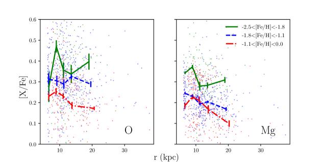
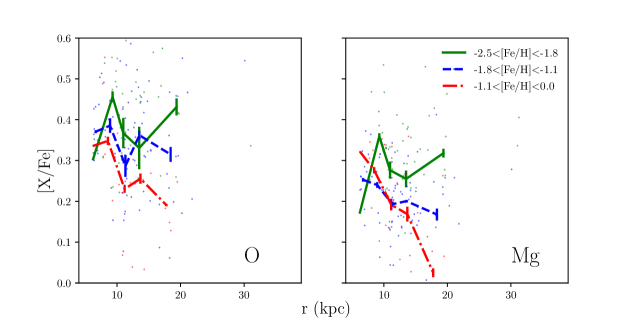
Figure 1: Top panels: Median [O/Fe] and [Mg/Fe] ratios determined for the selected whole sample in bins $r$ (from 5 kpc to 30 kpc) for stars in three different ranges in [Fe/H] ($-2.5<$ [Fe/H] $<-1.8$, $-1.8<$ [Fe/H] $<-1.1$, and -$1.1<$ [Fe/H] $<0.0$). The error bars are the statistical error for each median determined, the median absolute deviation (MAD). Bottom panels: Same as top panels but considering only stars with 4600 < $T_{\rm eff}$ < 4800 (reduced sample).

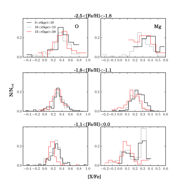
Figure 2: Distribution of [X/Fe] of the whole sample for each $r$ range (each histogram: 5 $<r<10$ kpc in black, 10 $<r<$ 15 kpc in grey, and 15 $<r<30$ kpc in red) at the three different [Fe/H] bins considered, from the first to the third rows of panels, respectively. The y-axis corresponds to the number of stars ($N$) in each [X/Fe] bin, normalized to the total number of stars ($N_{tot}$) in each bin of $r$ and [Fe/H].

We acknowledge the fact that these simulated haloes appear to be more massive than suggested by observations (Harmsen et al., 2017). In part, this could be due to an excess of in-situ stars or a misclassification of thick-disc stars as disc-heated stars. Depending on the halo, the in-situ fraction contributes about 30 per cent of the inner stellar halo (Tissera et al., 2012). A better agreement between observations and simulations is found if the in-situ components are not considered (Carollo et al., 2018). This is also the case for other simulations that have been performed with different numerical codes and baryonic physics (e.g. Monachesi et al., 2018). Nevertheless, the comparative analysis of the assembly histories and the $\alpha$-element patterns of these two haloes provides useful clues for the interpretation of the current observations, as they have been performed with the same subgrid physics and numerical resolution, being the initial conditions (i.e. assembly histories) the only difference between them.

In this paper, we focus on the simulated [O/Fe] distributions as a function of radius, which we take to be representative of [Mg/Fe] as well. The yields adopted for SNII are those of Woosley & Weaver (1995) and they have some issues with Mg so that they produce less elements than expected. However the O abundances are well-reproduced. As a consequence we decided to use O abundances for the simulations.

3 The analysis

3.1 Observed chemical patterns

We aim to properly study the [X/Fe] abundance variations across the halo for $\alpha$-elements, as a function of metallicity, which we identify with the [Fe/H] abundance ratio. We perform this analysis for the [O/Fe] and [Mg/Fe] abundances released in DR14. These two elements have a similar origin, and are mainly released into the interstellar medium through the explosion of Type II supernovae.

As in Fernández-Alvar et al. (2017), we calculate the median [X/Fe] from the abundances available in the DR14 catalogue in bins of distance from the Galactic center, $r$, of 2.5 kpc, assuring a minimum of 5 stars per bin. We calculate the medians for different metallicity ranges: $-2.5<$ [Fe/H] $<-1.8$ (low-metallicity population), $-1.8<$ [Fe/H] $<-1.1$ (intermediate-metallicity population), and $-1.1<$ [Fe/H] $<0.0$ (high-metallicity population).

The derived chemical trends for our entire halo sample are shown in Figure 1. The panels exhibit the resulting [X/Fe] medians, as well as their corresponding median absolute deviation (MAD), as a function of $r$.

The chemical trends for both elemental-abundance ratios exhibit a significant decrease with $r$ for stars at $-1.1<$ [Fe/H] $<0.0$. We first evaluate the possibility that this gradient is the result of our selection criteria. We obtain the $\log g$ distribution at each [Fe/H] and radial bin. We note that for $r>15$ kpc the $\log g$ distribution is skewed toward lower values (peak at $\log g\sim 1.0$), whereas at lower distances the distribution peaks at higher $\log g$ values. The [O/Fe] abundances do not show a trend with $\log g$, except a slightly increasing trend with $\log g$ in the $-1.1<$ [Fe/H] $<0.0$ bin at $r>15$ kpc. Stars in this bin exhibit lower [O/Fe] values at $\log g\sim 1.0$ than stars at $r<15$ kpc. However, this trend with $\log g$ is not observed in the case of [Mg/Fe], for which the decreasing trend of this ratio with distance is the same as observed for [O/Fe]. For this reason, we consider that the decrease detected for the [$\alpha$-elements/Fe] ratio with distance from the Galactic center is not due to the shift in the $\log g$ distribution toward lower values at the largest distances.

The oxygen abundances are determined from 50 regions of the spectra covering mostly OH molecular bands (Holtzman et al. 2018). The OH bands are very sensitive to the adopted $T_{\rm eff}$. We detect a bias in [Fe/H] towards high values at $T_{\rm eff}>$ 4600 K. We also detect an increasing trend of [O/Fe] with $T_{\rm eff}$, and an important increase in the abundance dispersion for stars with $T_{\rm eff}>5000$ K. [Mg/Fe] abundances also show an increasing trend with $T_{\rm eff}$, although much lower than for [O/Fe]. In order to avoid artificial distortions in the derived trends with distance due to these systematic effects, we reduce our sample to a narrower range of $T_{\rm eff}$, [4600 , 4800] K, where there is no bias toward higher [Fe/H] and no dependence of the chemical abundances with $T_{\rm eff}$ is observed. This reduced sample comprised 183 stars. The bottom panels in Fig. 1 show the resulting trends inferred from this smaller group. Due to the lower number of stars, the dispersion in the resulting median trends is larger and the statistical results are less robust. However, the trends inferred are qualitatively the same as those derived from the whole sample, in particular the steeper decreasing trend observed in the most metal-rich bin. The fact that we detected the same patterns with $r$ using a sample where the chemical abundances do not show systematic correlations with stellar parameters suggests that these trends are real, and not an artifact.

Figure 2 shows the [X/Fe] distribution in each of the [Fe/H] ranges considered, and three radial bins, $5<r<10$ kpc, $10<r<15$ kpc, and $15<r<30$ kpc, normalised to the total number of stars in each radial bin.

These trends, inferred from a larger number of halo stars and improved abundance determinations and distances, confirm the decrease in [$\alpha$/Fe] with $r$ for stars at [Fe/H] $>-1.1$ reported by Fernández-Alvar et al. (2017).

3.2 Simulated chemical trends

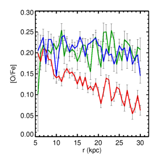
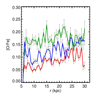
Figure 3: Median [O/Fe] values derived from the Aq-C (top panel) and the Aq-D (bottom panel) halos obtained from the Aquarius cosmological simulations, in the same [Fe/H] and $r$ bins, and using the same color coding, as the observations.

We estimated the [O/Fe] profiles for the seven Aquarius haloes (A, B, C, D, F, G, H) analysed by Tissera et al. (2012), calculating medians in the same [Fe/H] and $r$ intervals used for the observations. We only considered stars located at $|h|>5$ kpc, the same requirement imposed for the APOGEE observations. In the case of the simulations, ¹⁶O is our $\alpha$-element reference. After exploring the trends in all the haloes, we choose two of them to make a detailed analysis in relation to their assembly histories, Aq-C and Aq-D. The simulated halo that best represents the observational [O/Fe] and [Mg/Fe] trends shown in Fig.  1 is Aq-C, which exhibits a decrease in these trends with $r$ for the most metal-rich bin, stars with [Fe/H]$>-1.1$. On the contrary, the halo that differs the most from the observations is Aq-D, exhibiting a slightly increasing $\alpha$-enrichment with increasing radius. We show the trends for both haloes in Fig.3. From these figures, we also note that, for the intermediate-[Fe/H] interval, Aq-D also exhibits an increase of [O/Fe], while Aq-C has a flat trend with radius. In the low-[Fe/H] interval, the trends with radius are flat for both simulated haloes.

In order to further compare the observations and simulations, Fig. 4 shows the [O/Fe] distributions for the defined radial intervals. At first sight, the distributions appear different from the observed ones shown in Fig. 2. However, when examined in detail, some similarities emerge. In the case of Aq-C, the trends from the the inner to outer radii for the three metallicity sub-samples are similar: the inner radii are more dominated by $\alpha$-rich stars with respect to the $\alpha$-poor stars, principally in the outer radial interval. Althougth at all radii and metallicities, there is a larger contribution of $\alpha$-rich stars in Aq-C, the relative contribution of $\alpha$-poor stars increases remarkably for high metallicities in outer radial interval. It is this different relative contribution of $\alpha$-poor stas that results in a slope more comparable to the MW abundance patterns. A similar change in the relative contribution of $\alpha$-rich to $\alpha$-poor stars can be seen in Fig. 2. However, we acknowledge the fact that the observations show a sharper decrease of $\alpha$-rich and high-metallicity stars in the outer region than that predicted by Aq-C.

Conversely, Aq-D does not exhibit such a significant contribution from $\alpha$-rich stars in the high-metallicity interval at any radius, because there is a larger contribution of $\alpha$-poor stars at all radii. In addition, the contribution of $\alpha$-rich stars increases for $r>15$ kpc. This is why the median [O/Fe] in the central regions of Aq-D are lower than in the outer radial interval, producing the opposite trend to that found in Aq-C. Below we explore why this happens in Aq-D but not in Aq-C, the simulated halo that is most like the observed MW [O/Fe] pattern.

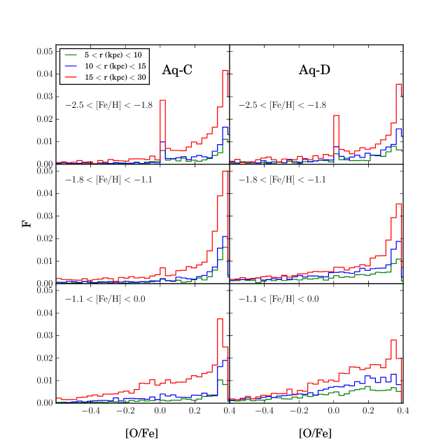
Figure 4: Mass fractions of stars within the three metallicity intervals: $-2.5<$ [Fe/H] $<-1.8$ (upper), $-1.8<$ [Fe/H] $<-1.1$ (middle), and $-1.1<$ [Fe/H] $<0.0$ (lower panels) and in three radial intervals: $5<r<10$ kpc (blue lines), $10<r<15$ kpc (green lines), and $15<r<30$ kpc (red lines), for haloes Aq-C and Aq-D (left and right columns, respectively), normalized to the total mass in each bin of $r$ and [Fe/H].

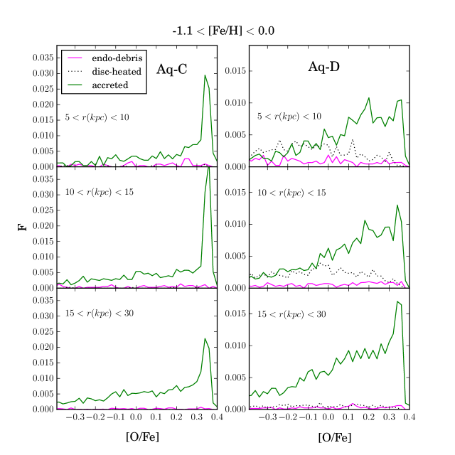
Figure 5: Mass fractions of stars, F, at $-1.1<$ [Fe/H]$<0.0$ in the three radial intervals: $5<r<10$ kpc (green lines), $10<r<15$ kpc (blue lines), and $15<r<30$ kpc (red lines), normalized to the total mass in this [Fe/H] bin, for haloes Aq-C and Aq-D (left and right columns, respectively), considering separately each sub-population with a different origin.

3.3 The high-metallicity stellar population

To understand which stellar populations (according to their origin) are responsible of the [O/Fe] gradient in stars with $-1.1<$ [Fe/H] $<0.0$, we examine the contribution of each sub-population according to their origin. We focus on this metallicity interval because it is the one which shows the strongest signature in the observations (see Fig. 1).

Figure 5 shows the contribution of the stellar populations to the [O/Fe] distributions for those stars with $-1.1<$ [Fe/H]$<0.0$, divided into the three defined radial intervals for the Aq-C and Aq-D simulated haloes. Each sub-sample has been normalised to the total stellar mass within a radial interval. This figure reveals that the Aq-C halo is characterised by a conspicuous fraction of accreted stars with high-[O/Fe] ($\sim+0.3$) for each $r$ interval. The contribution of in-situ stars is almost negligible compared with the contribution of accreted stars. The fraction of accreted stars with [O/Fe] $<+0.2$ increases with $r$, whereas that corresponding to high [O/Fe] decreases, causing the negative [O/Fe] gradient with $r$. Therefore, the stellar population responsible for the negative [O/Fe] gradient with distance is the large fraction of accreted stars with low $\alpha$-values.

In Aq-D, there is smaller relative contribution of accreted high-[O/Fe] stars. There is also a larger contribution of disc-heated stars with low [O/Fe]. This fraction of in-situ stars decreases as $r$ increases, so the contribution of stars with high [O/Fe] increases with $r$. In addition, the distribution of [O/Fe] is broader, without a strong peak at high [O/Fe], as in the case of Aq-C. The relative fraction of high-[O/Fe] stars tend to increase with $r$. Consequently, the median [O/Fe] value for stars within this metallicity range is higher, as they are located farther away. In this simulated halo, the $\alpha$-poor stars are more concentrated in the inner regions.

3.4 The assembly history behind the $\alpha$-element trends

In the case of Aq-C, the distribution of [O/Fe], with a peak at high [O/Fe] $\sim+0.35$ at high metallicities ([Fe/H] $>-1.1$), implies that these stars should have formed from a short and intense burst of star formation. The ISM would have reached large [Fe/H] and [O/H], both mainly due to the contribution of SNeII. The stars contributing to the nearer regions ($r<15$ kpc) should be old and contemporaneous, otherwise SNeIa would have had time to explode, enriching the ISM so that the subsequently born stars would have lower [O/Fe]. On the other hand, the increase of low [O/Fe] at more distant radii implies that these stars would be comparatively younger.

The broader distribution of [O/Fe] displayed by the accreted sample in the halo Aq-D, with a more similar fraction of low-[O/Fe] stars with respect to high-[O/Fe] stars, indicates that they would have formed during an extended star-formation era, allowing for a significant fraction of stars to be formed from gas enriched by SNeIa.

To further probe this hypothesis, we examine the age distribution of each stellar population. As can be seen from Fig. 6, the accreted stars in the halo Aq-C populating the nearer region are concentrated in an age range [$\sim 11.5,13.0$] Gyr. A secondary peak at $\sim 11$ Gyr, which would correspond to stars with lower [O/Fe] values, is considerably lower with respect to the rest of the distribution, but increases with increasing radii and extends towards lower ages. This age distribution explains the increment of low-[O/Fe] stars, which are indeed slightly younger stars, formed at an epoch when the ISM would have been already enriched by SNeIa. There is also a fraction of in-situ endo-debris stars peaked at $\sim 12$ Gyr for stars at $r<10$ kpc, which diminishes at higher radii.

Conversely, the distribution of stellar ages for the halo Aq-D peaks at slightly lower values, $\sim 11.5$ Gyr, and extends over the range [$\sim 9.5$, $\sim 13$] Gyr. These stars formed during a more extending period compared with Aq-C. From Fig. 7 we can also see that there are disc-heated stars with ages in the range [$\sim 7$, $\sim 9.5$] Gyr. In the intermediate radial range, there is also an significant contribution from disc-heated stars in this halo.

The main difference between the age distributions of the high-metallicity stars in Aq-C and Aq-D is that the former has older stellar populations in the inner regions, and in the outer radial interval the age distributions are consistent with two star-formation episodes. This is not the case for Aq-D, which exhibits a more extended period of star formation in all three radial intervals.

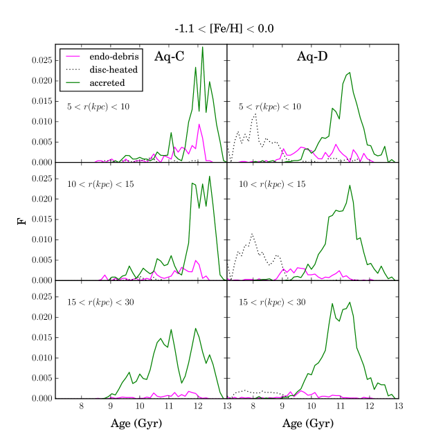
Figure 6: Distribution of simulated ages from the Aq-C and Aq-D haloes for each stellar population with different origin and [Fe/H] > -1.1. We show the distributions for each adopted radial interval as in Fig. 5.

3.5 Accreted satellites

To further understand the contributions of the accreted satellite galaxies to the formation of the inner regions of these haloes and, therefore, their role in setting the [O/Fe] profiles, Fig. 7 and Fig. 8 show the contribution of stars with different metallicities to the different radial intervals of the inner stellar haloes, by small (M $<10^{9}$M_⊙) , intermediate ($10^{9}$M${}_{\odot}<$ M $<10^{10}$M_⊙), and massive (M $>10^{10}$M_⊙) satellites (where M denotes the dynamical mass of the accreted satellites at the time it enters the virial radius of the main progenitor galaxy).

As shown in Fig. 7, Aq-C has a larger contribution from intermediate-mass satellites for the lower metallicity interval. The higher-metallicity accreted stars are formed in massive and intermediate-mass satellites. For increasing radius, the contributions from massive satellites increases. This is consistent with the previous trends showing these stars have lower [O/Fe] abundances. From figure 4 in Tissera et al. (2014), we know that the Aq-C inner region did not receive satellites larger than about $\sim 2\times 10^{10}$M_⊙. Our analysis shows that three satellites, with dynamical masses not larger than $2\times 10^{10}$ M_⊙, contribute stars particularly in the outer radial interval.

Regarding Aq-D, the trends in Fig. 8 show a different assembly history, with a more significant contribution coming from massive satellites, also in agreement with figure 4 in Tissera et al. (2014). These satellites are more massive, and contribute to all radial and metallicity intervals. These more massive satellite accretion affects the inner region and contributes less $\alpha$-enhanced stars to the inner radial bins. We identify contributions from up to four satellites with mean dynamical masses $\sim 2.5\times 10^{10}$M_⊙ (i.e., in the range [$\sim 2.5$ , $\sim 4.3\times 10^{10}$] M_⊙).

For both Aq-C and Aq-D, these satellites did not deposit all of their stars within these regions. There are partial contributions as the satellites are disrupted. In the case of Aq-D, the more-massive satellites contribute $\sim 75\%$, $\sim 66\%$, and $\sim 56\%$ of the stars in the high-, intermediate-, and low-metallicity populations. Conversely, for Aq-C, the higher-mass satellites contribute $\sim 39\%$, $\sim 28\%$, and $\sim 21\%$ for the same metallicity populations. However, this halo has the largest contributions coming from intermediate-mass satellites:$\sim 52\%$, $\sim 53\%$, and $\sim 47\%$ of the stars in the high-, intermediate-, and low-metallicity populations, respectively.

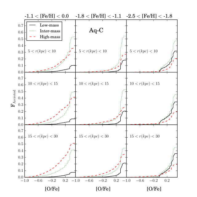
Figure 7: Mass-weighted distributions of the accreted stellar populations of Aq-C, grouped according to the mass of their host satellites, normalized to each $r$ and [Fe/H] bin. Accreted stars are shown according to different metallicity intervals (left:high-metallicity, middle: intermediate-metallicity, right: low-metallicity), and different radial intervals (upper: inner regions, middle: intermediate regions, lower panels: outer regions).

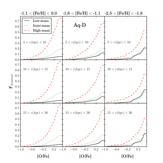
Figure 8: Mass-weighted distributions of the accreted stellar populations of Aq-D, grouped according to the mass of their host satellites, normalized to each $r$ and [Fe/H] bin. Accreted stars are shown according to different metallicity intervals (left:high-metallicity, middle: intermediate-metallicity, right: low-metallicity), and different radial intervals (upper: inner regions, middle: intermediate regions, lower panels: outer regions).

In summary, Aq-C shows a similar [$\alpha$/Fe] trend as a function of radius to the observations; it has been already reported that a late-infalling massive satellite with an extended SFH is contributing significant mass at intermediate distances – for a very detailed description of that satellite orbit see Parry et al. (2012) and Appendix A1 of Cooper et al. (2017). Aq-D shows the opposite trend, supporting the idea that incomplete mixing of a massive progenitor is responsible for what is observed in the MW.

In fact, considering recent observational results in the MW regarding the existence of remnants of accreted satellites in the stellar halo (Belokurov et al., 2018; Helmi et al., 2018), we carried out the exercise of selecting high-metallicity star particles with large radial velocities ($|v_{r}|>150$ km/s) and small tangential ones $|v_{t}|<30$ km/s, contributed by satellites of different masses in order to find out clues on their origins. We find that, in Aq-C, 50, 32 and 18 per cent of high-metallicity stars were contributed by massive, intermediate and small mass galaxies. While for Aq-D these percentages are 73, 19, and 7 per cent, respectively, in agreement with the trends shown in Fig.6 and Fig.7. It is clear that in both cases the majority of the high-metallicity stars are associated to massive satellites. However, in the case of Aq-D, the massive satellite clearly has the principal role. Nevertheless, this last halo do not have a distribution of $\alpha$-elements consistent with observations in the MW because most of the stars are $\alpha$-poor and they have been able to reach the center. So that the $\alpha$-profiles is inverted with respect to that of Aq-C. It is very interesting to take into account the results of Cooper et al. (2017) that tracked the satellite in time and found it has gone several pass-bye in the last 8 Gyrs. We cannot prevent the obvious question: in the case of the MW, could be the satellite responsible of imprinting this $\alpha$-pattern still around (e.g. Belokurov et al., 2018; Koposov et al., 2018)?

4 Conclusions

The elemental-abundance ratios for the two $\alpha$-elements O and Mg reported in the DR14 APOGEE/APOGEE-2 database for relatively metal-rich halo stars ([Fe/H] $>-1.1$) at Galactocentric radii between 5 and $\sim$30 kpc exhibit a gradient with distance, which becomes flatter at lower metallicity. The simulated halo that best reproduces this observational feature is Aq-C. This halo exhibits a decreasing trend in [O/Fe] with $r$ for stars at [Fe/H] $>-1.1$ and flat trends at lower [Fe/H], for stars at $r>5$ kpc, qualitatively similar to the [O/Fe] trends inferred from the APOGEE/APOGEE-2 DR14 observations.

The results from the comparative analysis of Aq-C and Aq-D indicates that the decreasing [O/Fe] with radius for more metal-rich stars is due to the contribution of accreted stars from satellite galaxies with about $10^{10}$ M$\sun$ dynamical mass that did not get all way to the central region. The assembly history for Aq-C is characterised by the larger contribution from intermediate-mass satellites in the inner regions ($r<15$ kpc) with old high-$\alpha$ stars, and the increase of the contribution from more-massive satellites, populating it with younger low-$\alpha$ stars, at $r>15$ kpc.

The large fraction of old high-[O/Fe] stars at $r<15$ kpc is due to short and intense bursts of star formation, while the low-[O/Fe] stellar populations are associated with a later second burst. There is a clear gap between the two starbursts, which provides enough time for SNIa enrichment. Note that these two $\alpha$-enriched populations might have formed in different accreted satellites.

An intermediate/massive satellite would be able to retain gas to have a second starburst, after the first one quenched star formation by heating up the ISM (Aq-C). However, if it is sufficiently massive, then the period of star formation would be more extended, and the satellite would also be able to reach the inner regions (Amorisco, 2017; Fattahi et al., 2018) as is the case in Aq-D. The resulting [O/Fe] patterns will be different: more enriched material would be able to reach the central region in the latter case, thus producing a positive increases of [O/Fe] with radius. Note that these satellites could also heat up the old disc, contributing with more disc-heated stars in the halo. Our results are in agreement with those recently reported in the literature pointing to the accretion of a relatively massive satellite. In particular, our results agree with Mackereth et al. (2018) who analysed simulated galaxies from the EAGLE project and inferred a merger history for the Milky Way of satellites with stellar masses in the range $10^{8}$-$10^{9}$M_⊙.

The comparative analysis between Aq-C and Aq-D we have carried out suggests that, in order to reproduce the observed $\alpha$-element patterns in the inner region of the MW, in particular the decrease of [O/Fe] for increasing radius, intermediate- and low-mass satellites would be expected to contribute to the very inner regions but a more-massive satellite (i.e., dynamical mass about $\sim 10^{10}$ M_⊙ at the time the satellite enters the virial radius of the MW progenitor) is expected to contribute low-$\alpha$ stars farther away. Considering our results and those of Cooper et al . (2017) we speculate that the surviving remnant of this massive satellite could be still orbiting the MW.

References

- Amorisco (2017) Amorisco N. C., 2017, MNRAS, 464, 2882
- Beers et al. (2012) Beers T. C., et al., 2012, ApJ, 746, 34
- Belokurov et al. (2006) Belokurov V., et al., 2006, ApJ, 642, L137
- Belokurov et al. (2018) Belokurov V., Erkal D., Evans N. W., Koposov S. E., Deason A. J., 2018, MNRAS, 478, 611
- Blanton et al. (2017) Blanton M. R., et al., 2017, AJ, 154, 28
- Bonaca et al. (2012) Bonaca A., et al., 2012, AJ, 143, 105
- Bonaca et al. (2017) Bonaca A., Conroy C., Wetzel A., Hopkins P. F., Kereš D., 2017, ApJ, 845, 101
- Bullock et al. (2010) Bullock J. S., Stewart K. R., Kaplinghat M., Tollerud E. J., Wolf J., 2010, ApJ, 717, 1043
- Carollo et al. (2007) Carollo D., et al., 2007, Nature, 450, 1020
- Carollo et al. (2010) Carollo D., et al., 2010, ApJ, 712, 692
- Carollo et al. (2018) Carollo D., Tissera P. B., Beers T. C., Gudin D., Gibson B. K., Freeman K. C., Monachesi A., 2018, ApJ, 859, L7
- Cooper et al. (2010) Cooper A. P., et al., 2010, MNRAS, 406, 744
- Cooper et al. (2015) Cooper A. P., Parry O. H., Lowing B., Cole S., Frenk C., 2015, MNRAS, 454, 3185
- Cooper et al. (2017) Cooper A. P., Cole S., Frenk C. S., Le Bret T., Pontzen A., 2017, MNRAS, 469, 1691
- Deason et al. (2018) Deason A. J., Belokurov V., Koposov S. E., Lancaster L., 2018, ApJ, 862, L1
- Eisenstein et al. (2011) Eisenstein D. J., et al., 2011, AJ, 142, 72
- Fattahi et al. (2018) Fattahi A., et al., 2018, arXiv e-prints,