Fast greedy algorithms for dictionary selection
with generalized sparsity constraints

Abstract

In dictionary selection, several atoms are selected from finite candidates that successfully approximate given data points in the sparse representation. We propose a novel efficient greedy algorithm for dictionary selection. Not only does our algorithm work much faster than the known methods, but it can also handle more complex sparsity constraints, such as average sparsity. Using numerical experiments, we show that our algorithm outperforms the known methods for dictionary selection, achieving competitive performances with dictionary learning algorithms in a smaller running time.

1 Introduction

Learning sparse representations of data and signals has been extensively studied for the past decades in machine learning and signal processing [16]. In these methods, a specific set of basis signals (atoms), called a dictionary, is required and used to approximate a given signal in a sparse representation. The design of a dictionary is highly nontrivial, and many studies have been devoted to the construction of a good dictionary for each signal domain, such as natural images and sounds. Recently, approaches to construct a dictionary from data have shown the state-of-the-art results in various domains. The standard approach is called dictionary learning [3, 32, 1]. Although many studies have been devoted to dictionary learning, it is usually difficult to solve, requiring a non-convex optimization problem that often suffers from local minima. Also, standard dictionary learning methods (e.g., MOD [14] or $k$-SVD [2]) require a heavy time complexity.

Krause and Cevher [22] proposed a combinatorial analogue of dictionary learning, called dictionary selection. In dictionary selection, given a finite set of candidate atoms, a dictionary is constructed by selecting a few atoms from the set. Dictionary selection could be faster than dictionary learning due to its discrete nature. Another advantage of dictionary selection is that the approximation guarantees hold even in agnostic settings, i.e., we do not need stochastic generating models of the data. Furthermore, dictionary selection algorithms can be used for media summarization, in which the atoms must be selected from given data points [8, 9].

The basic dictionary selection is formalized as follows. Let $V$ be a finite set of candidate atoms and $n=\lvert V\rvert$. Throughout the paper, we assume that the atoms are unit vectors in $\mathbb{R}^{d}$ without loss of generality. We represent the candidate atoms as a matrix $\mathbf{A}\in\mathbb{R}^{d\times n}$ whose columns are the atoms in $V$. Let $\mathbf{y}_{t}\in\mathbb{R}^{d}$ ($t\in[T]$) be data points, where $[T]=\{1,\dots,T\}$, and $k$ and $s$ be positive integers with $k\geq s$. We assume that a utility function $u:\mathbb{R}^{d}\times\mathbb{R}^{d}\to\mathbb{R}_{+}$ exists, which measures the similarity of the input vectors. For example, one can use the $\ell^{2}$-utility function $u(\mathbf{y},\mathbf{x})=\lVert\mathbf{y}\rVert_{2}^{2}-\lVert\mathbf{y}-\mathbf{x}\rVert_{2}^{2}$ as in Krause and Cevher [22]. Then, the dictionary selection finds a set $X\subseteq V$ of size $k$ that maximizes

$$h(X)=\sum_{t=1}^{T}\max_{\mathbf{w}\in\mathbb{R}^{k}\colon\lVert\mathbf{w}\rVert_{0}\leq s}u(\mathbf{y}_{t},\mathbf{A}_{X}\mathbf{w}),$$ (1)

where $\lVert\mathbf{w}\rVert_{0}$ is the number of nonzero entries in $\mathbf{w}$ and $\mathbf{A}_{X}$ is the column submatrix of $\mathbf{A}$ with respect to $X$. That is, we approximate a data point $\mathbf{y}_{t}$ with a sparse representation in atoms in $X$, where the approximation quality is measured by $u$. Letting $f_{t}(Z_{t}):=\max_{\mathbf{w}}u(\mathbf{y}_{t},\mathbf{A}_{Z_{t}}\mathbf{w})$ ($t\in[T]$), we can rewrite this as the following two-stage optimization: $h(X)=\sum_{t=1}^{T}\max_{Z_{t}\subseteq X\colon\lvert Z_{t}\rvert\leq s}f_{t}(Z_{t})$. Here $Z_{t}$ is the set of atoms used in a sparse representation of data point $\mathbf{y}_{t}$. The main challenges in dictionary selection are that the evaluation of $h$ is NP-hard in general [25], and the objective function $h$ is not submodular [17] and therefore the well-known greedy algorithm [27] cannot be applied. The previous approaches construct a good proxy of dictionary selection that can be easily solved, and analyze the approximation ratio.

1.1 Our contribution

Our main contribution is a novel and efficient algorithm called the replacement orthogonal matching pursuit (Replacement OMP) for dictionary selection. This algorithm is based on a previous approach called Replacement Greedy [30] for two-stage submodular maximization, a similar problem to dictionary selection. However, the algorithm was not analyzed for dictionary selection. We extend their approach to dictionary selection in the present work, with an additional improvement that exploits techniques in orthogonal matching pursuit. We compare our method with the previous methods in Table 1. Replacement OMP has a smaller running time than $\textsf{SDS}_{\textsf{OMP}}$ [10] and Replacement Greedy. The only exception is $\textsf{SDS}_{\textsf{MA}}$ [10], which intuitively ignores any correlation of the atoms. In our experiment, we demonstrate that Replacement OMP outperforms $\textsf{SDS}_{\textsf{MA}}$ in terms of test residual variance. We note that the constant approximation ratios of $\textsf{SDS}_{\textsf{MA}}$, Replacement Greedy, and Replacement OMP are incomparable in general. In addition, we demonstrate that Replacement OMP achieves a competitive performance with dictionary learning algorithms in a smaller running time, in numerical experiments.

Generalized sparsity constraint

Incorporating further prior knowledge on the data domain often improves the quality of dictionaries [28, 29, 11]. A typical example is a combinatorial constraint independently imposed on each support $Z_{t}$. This can be regarded as a natural extension of the structured sparsity [19] in sparse regression, which requires the support to satisfy some combinatorial constraint, rather than a cardinality constraint. A global structure of supports is also useful prior information. Cevher and Krause [6] proposed a global sparsity constraint called the average sparsity, in which they add a global constraint $\sum_{t=1}^{T}\lvert Z_{t}\rvert\leq s^{\prime}$. Intuitively, the average sparsity constraint requires that the most data points can be represented by a small number of atoms. If the data points are patches of a natural image, most patches are a simple background, and therefore the number of the total size of the supports must be small. The average sparsity has been also intensively studied in dictionary learning [11]. To deal with these generalized sparsities in a unified manner, we propose a novel class of sparsity constraints, namely $p$-replacement sparsity families. We prove that Replacement OMP can be applied for the generalized sparsity constraint with a slightly worse approximation ratio. We emphasize that the OMP approach is essential for efficiency; in contrast, Replacement Greedy cannot be extended to the average sparsity setting because it can only handle local constraints on $Z_{t}$, and yields an exponential running time.

Table 1: Comparison of known methods with Replacement OMP. The constants $m_{s}$, $M_{s}$, and $M_{s,2}$ are the restricted concavity and smoothness constants of $u(\mathbf{y}_{t},\cdot)$ ($t\in[T]$); see Section 2. The running time is from the $\ell^{2}$-utility function $u$ and the individual sparsity constraint.

Method	Approximation ratio	Running time	Generalized sparsity
$\textsf{SDS}_{\textsf{MA}}$ [22]	$\frac{m_{1}m_{s}}{M_{1}M_{s}}(1-1/\mathrm{e})$ [10]	$\mathrm{O}((k+d)nT)$	No
$\textsf{SDS}_{\textsf{OMP}}$ [22]	$\mathrm{O}(1/k)$ [10]	$\mathrm{O}((s+k)sdknT)$	No
Replacement Greedy [30]	$\left(\frac{m_{2s}}{M_{s,2}}\right)^{2}\left(1-\exp\left(-\frac{M_{s,2}}{m_{2s}}\right)\right)$	$\mathrm{O}(s^{2}dknT)$	No
this paper	$\left(\frac{m_{2s}}{M_{s,2}}\right)^{2}\left(1-\exp\left(-\frac{M_{s,2}}{m_{2s}}\right)\right)$	$\mathrm{O}((n+ds)kT)$	Yes

Online extension

In some practical situations, it is not always feasible to store all data points $\mathbf{y}_{t}$, but these data points arrive in an online fashion. We show that Replacement OMP can be extended to the online setting, with a sublinear approximate regret. The details are given in Section 5.

1.2 Related work

Krause and Cevher [22] first introduced dictionary selection as a combinatorial analogue of dictionary learning. They proposed $\textsf{SDS}_{\textsf{MA}}$ and $\textsf{SDS}_{\textsf{OMP}}$, and analyzed the approximation ratio using the coherence of the matrix $\mathbf{A}$. Das and Kempe [10] introduced the concept of the submodularity ratio and refined the analysis via the restricted isometry property [5]. A connection to the restricted concavity and submodularity ratio has been investigated by Elenberg et al. [13], Khanna et al. [21] for sparse regression and matrix completion. Balkanski et al. [4] studied two-stage submodular maximization as a submodular proxy of dictionary selection, devising various algorithms. Stan et al. [30] proposed Replacement Greedy for two-stage submodular maximization. It is unclear that these methods provide an approximation guarantee for the original dictionary selection.

To the best of our knowledge, there is no existing research in the literature that addresses online dictionary selection. For a related problem in sparse optimization, namely online linear regression, Kale et al. [20] proposed an algorithm based on supermodular minimization [23] with a sublinear approximate regret guarantee. Elenberg et al. [12] devised a streaming algorithm for weak submodular function maximization. Chen et al. [7] dealt with online maximization of weakly DR-submodular functions.

Organization

The rest of this paper is organized as follows. Section 2 provides the basic concepts and definitions. Section 3 formally defines dictionary selection with generalized sparsity constraints. Section 4 presents our algorithm, Replacement OMP. Section 5 sketches the extension to the online setting. The experimental results are presented in Section 6.

2 Preliminaries

Notation

For a positive integer $n$, $[n]$ denotes the set $\{1,2,\dots,n\}$. The sets of reals and nonnegative reals are denoted by $\mathbb{R}$ and $\mathbb{R}_{\geq 0}$, respectively. We similarly define $\mathbb{Z}$ and $\mathbb{Z}_{\geq 0}$. Vectors and matrices are denoted by lower and upper case letters in boldface, respectively: $\mathbf{a},\mathbf{x},\mathbf{y}$ for vectors and $\mathbf{A},\mathbf{X},\mathbf{Y}$ for matrices. The $i$th standard unit vector is denoted by $\mathbf{e}_{i}$; that is, $\mathbf{e}_{i}$ is the vector such that its $i$th entry is equal to one and all other entries are zero. For a matrix $\mathbf{A}\in\mathbb{R}^{d\times n}$ and $X\subseteq[n]$, $\mathbf{A}_{X}$ denotes the column submatrix of $\mathbf{A}$ with respect to $X$. The maximum and minimum singular values of a matrix $\mathbf{A}$ are denoted by $\sigma_{\mathrm{max}}(\mathbf{A})$ and $\sigma_{\mathrm{min}}(\mathbf{A})$, respectively. For a positive integer $k$, we define $\sigma_{\mathrm{max}}(\mathbf{A},k)\coloneqq\max_{X\subseteq[n]\colon\lvert X\rvert\leq k}\sigma_{\mathrm{max}}(\mathbf{A}_{X})$. We define $\sigma_{\mathrm{min}}(\mathbf{A},k)$ in a similar way. For $t\in[T]$, let $u_{t}(\mathbf{w}):=u(\mathbf{y}_{t},\mathbf{A}\mathbf{w})$. Let $\mathbf{w}^{(Z_{t})}_{t}$ denote the maximizer of $u_{t}(\mathbf{w})$ subject to $\mathrm{supp}(\mathbf{w})\subseteq Z_{t}$. Throughout the paper, $V$ denotes the fixed finite ground set. For $X\subseteq V$ and $a\in V\setminus X$, we define $X+a\coloneqq X\cup\{a\}$. Similarly, for $a\in V\setminus X$ and $b\in X$, we define $X-b+a\coloneqq(X\setminus\{b\})\cup\{a\}$.

2.1 Restricted concavity and smoothness

The following concept of restricted strong concavity and smoothness is crucial in our analysis.

Definition 2.1 (Restricted strong concavity and restricted smoothness [26]).

Let $\Omega$ be a subset of $\mathbb{R}^{d}\times\mathbb{R}^{d}$ and $u\colon\mathbb{R}^{d}\to\mathbb{R}$ be a continuously differentiable function. We say that $u$ is restricted strongly concave with parameter $m_{\Omega}$ and restricted smooth with parameter $M_{\Omega}$ if,

$$-\frac{m_{\Omega}}{2}\lVert\mathbf{y}-\mathbf{x}\rVert_{2}^{2}\geq u(\mathbf{y})-u(\mathbf{x})-\langle\nabla u(\mathbf{x}),\mathbf{y}-\mathbf{x}\rangle\geq-\frac{M_{\Omega}}{2}\lVert\mathbf{y}-\mathbf{x}\rVert^{2}_{2}$$

for all $(\mathbf{x},\mathbf{y})\in\Omega$.

We define $\Omega_{s,p}\coloneqq\{(\mathbf{x},\mathbf{y})\in\mathbb{R}^{d}\times\mathbb{R}^{d}\colon\lVert\mathbf{x}\rVert_{0},\lVert\mathbf{y}\rVert_{0}\leq s,\lVert\mathbf{x}-\mathbf{y}\rVert_{0}\leq p\}$ and $\Omega_{s}\coloneqq\Omega_{s,s}$ for positive integers $s$ and $p$. We often abbreviate $M_{\Omega_{s}}$, $M_{\Omega_{s,p}}$, and $m_{\Omega_{s}}$ as $M_{s}$, $M_{s,p}$, and $m_{s}$, respectively.

3 Dictionary selection with generalized sparsity constraints

In this section, we formalize our problem, dictionary selection with generalized sparsity constraints. In this setting, the supports $Z_{t}$ for each $t\in[T]$ cannot be independently selected, but we impose a global constraint on them. We formally write such constraints as a down-closed  family $\mathcal{I}\subseteq\prod_{t=1}^{T}2^{V}$. Therefore, we aim to find $X\subseteq V$ with $\lvert X\rvert\leq k$ maximizing

$$h(X)=\max_{Z_{1},\dots,Z_{t}\subseteq X\mid(Z_{1},\dots,Z_{t})\in\mathcal{I}}\sum_{t=1}^{T}f_{t}(Z_{t})$$ (2)

Since a general down-closed family is too abstract, we focus on the following class. First, we define the set of feasible replacements for the current support $Z_{1},\cdots,Z_{T}$ and an atom $a$ as

$$\mathcal{F}_{a}(Z_{1},\cdots,Z_{T})=\left\{(Z^{\prime}_{1},\cdots,Z^{\prime}_{T})\in\mathcal{I}\mid Z^{\prime}_{t}\subseteq Z_{T}+a,\,|Z_{t}\setminus Z^{\prime}_{t}|\leq 1~{}(\forall t\in[T])\right\}.$$ (3)

That is, the set of members in $\mathcal{I}$ obtained by adding $a$ and removing at most one element from each $Z_{t}$. Let $\mathcal{F}(Z_{1},\cdots,Z_{T})=\bigcup_{a\in V}\mathcal{F}_{a}(Z_{1},\cdots,Z_{T})$. If $Z_{1},\dots,Z_{T}$ are clear from the context, we simply write it as $\mathcal{F}_{a}$.

Definition 3.1 ($p$-replacement sparsity).

A sparsity constraint $\mathcal{I}\subseteq\prod_{t=1}^{T}2^{V}$ is $p$-replacement sparse if for any $(Z_{1},\dots,Z_{T}),(Z_{1}^{*},\dots,Z_{T}^{*})\in\mathcal{I}$, there is a sequence of $p$ feasible replacements $(Z^{p^{\prime}}_{1},\dots,Z^{p^{\prime}}_{T})\in\mathcal{F}(Z_{1},\dots,Z_{T})$ ($p^{\prime}\in[p]$) such that each element in $Z^{*}_{t}\setminus Z_{t}$ appears at least once in the sequence $(Z^{p^{\prime}}_{t}\setminus Z_{t})_{p^{\prime}=1}^{p}$ and each element in $Z_{t}\setminus Z_{t}^{*}$ appears at most once in the sequence $(Z_{t}\setminus Z^{p^{\prime}}_{t})_{p^{\prime}=1}^{p}$.

The following sparsity constraints are all $p$-replacement sparsity families. See Appendix B for proof.

Example 3.2 (individual sparsity).

The sparsity constraint for the standard dictionary selection can be written as $\mathcal{I}=\{(Z_{1},\cdots,Z_{T})\mid|Z_{t}|\leq s~{}(\forall t\in[T])\}$. We call it the individual sparsity constraint. This constraint is a special case of an individual matroid constraint, described below.

Example 3.3 (individual matroids).

This was proposed by [30] as a sparsity constraint for two-stage submodular maximization. An individual matroid constraint can be written as $\mathcal{I}=\{(Z_{1},\cdots,Z_{T})\mid Z_{t}\in\mathcal{I}_{t}~{}(\forall t\in[T])\}$ where $(V,\mathcal{I}_{t})$ is a matroid for each $t\in[T]$. An individual sparsity constraint is a special case of an individual matroid constraint where $(V,\mathcal{I}_{t})$ is the uniform matroid for all $t$.

Example 3.4 (block sparsity).

Block sparsity was proposed by Krause and Cevher [22]. This sparsity requires that the support must be sparse within each prespecified block. That is, disjoint blocks $B_{1},\cdots,B_{b}\subseteq[T]$ of data points are given in advance, and an only small subset of atoms can be used in each block. Formally, $\mathcal{I}=\{(Z_{1},\cdots,Z_{T})\mid|\bigcup_{t\in B_{b^{\prime}}}Z_{t}|\leq s_{b^{\prime}}~{}(\forall b^{\prime}\in[b])\}$ where $s_{b^{\prime}}\in\mathbb{Z}_{+}$ for each $b^{\prime}\in[b]$ are sparsity parameters.

Example 3.5 (average sparsity [6]).

This sparsity imposes a constraint on the average number of used atoms among all data points. The number of atoms used for each data point is also restricted. Formally, $\mathcal{I}=\{(Z_{1},\cdots,Z_{T})\mid|Z_{t}|\leq s_{t},\sum_{t=1}^{T}|Z_{t}|\leq s^{\prime}\}$ where $s_{t}\in\mathbb{Z}_{+}$ for each $t\in[T]$ and $s^{\prime}\in\mathbb{Z}_{+}$ are sparsity parameters.

Proposition 3.6.

The replacement sparsity parameters of individual matroids, block sparsity, and average sparsity are upper-bounded by $k$, $k$, and $3k-1$, respectively.

4 Algortihms

In this section, we present Replacement Greedy [30] and Replacement OMP for dictionary selection with generalized sparsity constraints.

4.1 Replacement Greedy

Replacement Greedy was first proposed as an algorithm for a different problem, two-stage submodular maximization [4]. In two-stage submodular maximization, the goal is to maximize

$$h(X)=\sum_{t=1}^{T}\max_{Z_{t}\subseteq X\colon Z_{t}\in\mathcal{I}_{t}}f_{t}(Z_{t}),$$ (4)

where $f_{t}$ is a nonnegative monotone submodular function ($t\in[T]$) and $\mathcal{I}_{t}$ is a matroid. Despite the similarity of the formulation, in dictionary selection, the functions $f_{t}$ are not necessarily submodular, but come from the continuous function $u_{t}$. Furthermore, in two-stage submodular maximization, the constraints on $Z_{t}$ are individual for each $t\in[T]$, while we pose a global constraint $\mathcal{I}$. In the following, we present an adaptation of Replacement Greedy to dictionary selection with generalized sparsity constraints.

Replacement Greedy stores the current dictionary $X$ and supports $Z_{t}\subseteq X$ such that $(Z_{1},\dots,Z_{T})\in\mathcal{I}$, which are initialized as $X=\varnothing$ and $Z_{t}=\varnothing$ ($t\in[T]$). At each step, the algorithm considers the gain of adding an element $a\in V$ to $X$ with respect to each function $f_{t}$, i.e., the algorithm selects $a$ that maximizes $\max_{(Z_{1}^{\prime},\dots,Z_{T}^{\prime})\in\mathcal{F}_{a}}\sum_{t=1}^{T}\{f_{t}(Z_{t}^{\prime})-f(Z_{t})\}$. See Algorithm 1 for a pseudocode description. Note that for the individual matroid constraint $\mathcal{I}$, the algorithm coincides with the original Replacement Greedy [30].

Algorithm 1 Replacement Greedy & Replacement OMP

1:  Initialize $X\leftarrow\varnothing$ and $Z_{t}\leftarrow\varnothing$ for $t=1,\dots,T$.

2:  for $i=1,\dots,k$ do

3:     Pick $a^{*}\in V$ that maximizes$\begin{cases}\max_{(Z^{\prime}_{1},\cdots,Z^{\prime}_{T})\in\mathcal{F}_{a^{*}}}\sum_{t=1}^{T}\left\{f_{t}(Z^{\prime}_{t})-f_{t}(Z_{t})\right\}\quad\text{({Replacement Greedy}{})}\\ \max_{(Z^{\prime}_{1},\cdots,Z^{\prime}_{T})\in\mathcal{F}_{a^{*}}}\left\{\frac{1}{M_{s,2}}\sum_{t=1}^{T}\lVert\nabla u_{t}(\mathbf{w}^{(Z_{t})}_{t})_{Z^{\prime}_{t}\setminus Z_{t}}\rVert^{2}-M_{s,2}\sum_{t=1}^{T}\lVert(\mathbf{w}^{(Z_{t})}_{t})_{Z_{t}\setminus Z^{\prime}_{t}}\rVert^{2}\right\}\\ \end{cases}$ (Replacement OMP)and let $(Z^{\prime}_{1},\cdots,Z^{\prime}_{T})$ be a replacement achieving a maximum.

4:     Set $X\leftarrow X+a^{*}$ and $Z_{t}\leftarrow Z^{\prime}_{t}$ for each $t\in[T]$.

5:  return $X$.

Stan et al. [30] showed that Replacement Greedy achieves an $((1-1/\sqrt{e})/2)$-approximation when $f_{t}$ are monotone submodular. We extend their analysis to our non-submodular setting. The proof can be found in Appendix C.

Theorem 4.1.

Assume that $u_{t}$ is $m_{2s}$-strongly concave on $\Omega_{2s}$ and $M_{s,2}$-smooth on $\Omega_{s,2}$ for $t\in[T]$ and that the sparsity constraint $\mathcal{I}$ is $p$-replacement sparse. Let $(Z_{1}^{*},\cdots,Z_{T}^{*})\in\mathcal{I}$ be optimal supports of an optimal dictionary $X^{*}$. Then the solution $(Z_{1},\cdots,Z_{T})\in\mathcal{I}$ of Replacement Greedy after $k^{\prime}$ steps satisfies

$$\sum_{t=1}^{T}f_{t}(Z_{t})\geq\frac{m^{2}_{2s}}{M_{s,2}^{2}}\left(1-\exp\left(-\frac{k^{\prime}}{p}\frac{M_{s,2}}{m_{2s}}\right)\right)\sum_{t=1}^{T}f_{t}(Z^{*}_{t})$$

4.2 Replacement OMP

Now we propose our algorithm, Replacement OMP. A down-side of Replacement Greedy is its heavy computation: in each greedy step, we need to evaluate $\sum_{t=1}^{T}f_{t}(Z_{t}^{\prime})$ for each $(Z_{1}^{\prime},\dots,Z_{t}^{\prime})\in\mathcal{F}_{a}(Z_{1},\dots,Z_{t})$, which amounts to solving linear regression problems $snT$ times if $u$ is the $\ell^{2}$-utility function. To avoid heavy computation, we propose a proxy of this quantity by borrowing an idea from orthogonal matching pursuit. Replacement OMP selects an atom $a\in V$ that maximizes

$$\max_{(Z^{\prime}_{1},\cdots,Z^{\prime}_{T})\in\mathcal{F}_{a}(Z_{1},\cdots,Z_{T})}\left\{\frac{1}{M_{s,2}}\sum_{t=1}^{T}\lVert\nabla u_{t}(\mathbf{w}^{(Z_{t})}_{t})_{Z^{\prime}_{t}\setminus Z_{t}}\rVert^{2}-M_{s,2}\sum_{t=1}^{T}\lVert(\mathbf{w}^{(Z_{t})}_{t})_{Z_{t}\setminus Z^{\prime}_{t}}\rVert^{2}\right\}.$$ (5)

This algorithm requires the smoothness parameter $M_{s,2}$ before the execution. Computing $M_{s,2}$ is generally difficult, but this parameter for the squared $\ell^{2}$-utility function can be bounded by $\sigma_{\mathrm{max}}^{2}(\mathbf{A},2)$. This value can be computed in $O(n^{2}d)$ time.

Theorem 4.2.

Assume that $u_{t}$ is $m_{2s}$-strongly concave on $\Omega_{2s}$ and $M_{s,2}$-smooth on $\Omega_{s,2}$ for $t\in[T]$ and that the sparsity constraint $\mathcal{I}$ is $p$-replacement sparse. Let $(Z_{1}^{*},\cdots,Z_{T}^{*})\in\mathcal{I}$ be optimal supports of an optimal dictionary $X^{*}$. Then the solution $(Z_{1},\cdots,Z_{T})\in\mathcal{I}$ of Replacement OMP after $k^{\prime}$ steps satisfies

$$\sum_{t=1}^{T}f_{t}(Z_{t})\geq\frac{m^{2}_{2s}}{M_{s,2}^{2}}\left(1-\exp\left(-\frac{k^{\prime}}{p}\frac{M_{s,2}}{m_{2s}}\right)\right)\sum_{t=1}^{T}f_{t}(Z^{*}_{t}).$$

4.3 Complexity

Now we analyze the time complexity of Replacement Greedy and Replacement OMP. In general, $\mathcal{F}_{a}$ has $O(n^{T})$ members, and therefore it is difficult to compute $\mathcal{F}_{a}$. Nevertheless, we show that Replacement OMP can run much faster for the examples presented in Section 3.

In Replacement Greedy, it is difficult to find an atom with the largest gain at each step. This is because we need to maximize a nonlinear function $\sum_{t=1}^{T}f_{t}(Z_{t}^{\prime})$. Conversely, in Replacement OMP, if we can calculate $\mathbf{w}^{(Z_{t})}_{t}$ and $\nabla u_{t}(\mathbf{w}^{(Z_{t})}_{t})$ for all $t\in[T]$, the problem of calculating gain of each atom is reduced to maximizing a linear function.

In the following, we consider the $\ell_{2}$-utility function and average sparsity constraint because it is the most complex constraint. A similar result holds for the other examples. In fact, we show that this task reduces to maximum weighted bipartite matching. The Hungarian method returns the maximum weight bipartite matching in $\mathrm{O}(T^{3})$ time. We can further improve the running time to $O(T\log T)$ time by utilizing the structure of this problem. Due to the limitation of space, we defer the details to Appendix C. In summary, we obtain the following:

Theorem 4.3.

Assume that the assumption of Theorem 4.2 holds. Further assume that $u$ is the $\ell^{2}$-utility function and $\mathcal{I}$ is the average sparsity constraint. Then Replacement OMP finds the solution $(Z_{1},\cdots,Z_{T})\in\mathcal{I}$

$$\sum_{t=1}^{T}f_{t}(Z_{t})\geq\left(\frac{\sigma_{\mathrm{max}}^{2}(\mathbf{A},2s)}{\sigma_{\mathrm{min}}^{2}(\mathbf{A},2)}\right)^{2}\left(1-\exp\left(-\frac{1}{3}\frac{\sigma_{\mathrm{min}}^{2}(\mathbf{A},2)}{\sigma_{\mathrm{max}}^{2}(\mathbf{A},2s)}\right)\right)\sum_{t=1}^{T}f_{t}(Z^{*}_{t})$$

in $O(Tk(n\log T+ds))$ time.

Remark 4.4.

If finding an atom with the largest gain is computationally intractable, we can add an atom whose gain is no less than $\tau$ times the largest gain. In this case, we can bound the approximation ratio with replacing $k^{\prime}$ with $\tau k^{\prime}$ in Theorem 4.1 and 4.2.

5 Extensions to the online setting

Our algorithms can be extended to the following online setting. The problem is formalized as a two-player game between a player and an adversary. At each round $t=1,\dots,T$, the player must select (possibly in a randomized manner) a dictionary $X_{t}\subseteq V$ with $\lvert X_{t}\rvert\leq k$. Then, the adversary reveals a data point $\mathbf{y}_{t}\in\mathbb{R}^{d}$ and the player gains $f_{t}(X_{t})=\max_{\mathbf{w}\in\mathbb{R}^{k}:\lVert\mathbf{w}\rVert_{0}\leq s}u(\mathbf{y}_{t},\mathbf{A}_{X}\mathbf{w})$. The performance measure of a player’s strategy is the expected $\alpha$-regret:

$$\operatorname{regret}_{\alpha}(T)=\alpha\max_{X^{*}:\lvert X^{*}\rvert\leq k}\sum_{t=1}^{T}f_{t}(X^{*})-\operatorname*{\mathbf{E}}\left[\sum_{t=1}^{T}f_{t}(X_{t})\right],$$

where $\alpha>0$ is a constant independent from $T$ corresponding to the offline approximation ratio, and the expectation is taken over the randomness in the player.

For this online setting, we present an extension of Replacement Greedy and Replacement OMP with sublinear $\alpha$-regret, where $\alpha$ is the corresponding offline approximation ratio. The details are provided in Appendix D.

6 Experiments

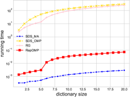
(a) synthetic, $T=100$, time

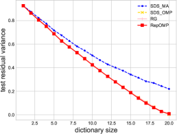
(b) synthetic, $T=100$, residual

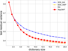
(c) voc, $T=100$, residual

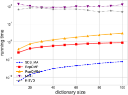
(d) synthetic, $T=1000$, time

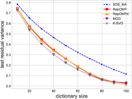
(e) synthetic, $T=1000$, residual

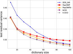
(f) voc, $T=1000$, residual

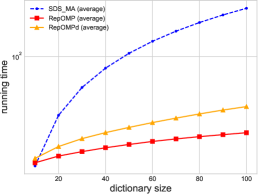
(g) synthetic, $T=1000$, time

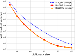
(h) synthetic, $T=1000$, residual

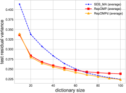
(i) voc, $T=1000$, residual

Figure 1: The experimental results for the offline setting. In all figures, the horizontal axis indicates the size of the output dictionary. 1(a), 1(b), and 1(c) are the results for $T=100$. 1(d), 1(e), and 1(f) are the results for $T=1000$. 1(g), 1(h), and 1(i) are the results for $T=1000$ with an average sparsity constraint. For each setting, we provide the plot of the running time for the synthetic dataset, test residual variance for the synthetic dataset, and test residual variance for VOC2006 image dataset.

In this section, we empirically evaluate our proposed algorithms on several dictionary selection problems with synthetic and real-world datasets. We use the squared $\ell^{2}$-utility function for all of the experiments. Since evaluating the value of the objective function is NP-hard, we plot the approximated residual variance obtained by orthogonal matching pursuit.

Ground set

We use the ground set consisting of several orthonormal bases that are standard choices in signal and image processing, such as 2D discrete cosine transform and several 2D discrete wavelet transforms (Haar, Daubechies 4, and coiflet). In all of the experiments, the dimension is set to $d=64$, which corresponds to images of size $8\times 8$ pixels. The size of the ground set is $n=256$.

Machine

All the algorithms are implemented in Python 3.6. We conduct the experiments in a machine with Intel Xeon E3-1225 V2 (3.20 GHz and 4 cores) and 16 GB RAM.

Datasets

We conduct experiments on two types of datasets. The first one is a synthetic dataset. In each trial, we randomly pick a dictionary with size $k$ out of the ground set, and generate sparse linear combinations of the columns of this dictionary. The weights of the linear combinations are generated from the standard normal distribution. The second one is a dataset of real-world images extracted from PASCAL VOC2006 image datasets [15]. In each trial, we randomly select an image out of 2618 images and divide it into patches of $8\times 8$ pixels, then select $T$ patches uniformly at random. All the patches are normalized to zero mean and unit variance. We make datasets for training and test in the same way, and use the training dataset for obtaining a dictionary and the test dataset for measuring the quality of the output dictionary.

6.1 Experiments on the offline setting

We implement our proposed methods, Replacement Greedy (RG) and Replacement OMP (ROMP), as well as the existing methods for dictionary selection, $\textsf{SDS}_{\textsf{MA}}$ and $\textsf{SDS}_{\textsf{OMP}}$. We also implement a heuristically modified version of ROMP, which we call ROMPd. In ROMPd, we replace $M_{s,2}$ with some parameter that decreases as the size of the current dictionary grows, which prevents the gains of all the atoms from being zero. Here we use $M_{s,2}/\sqrt{i}$ as the decreasing parameter where $i$ is the number of iterations so far. In addition, we compare these methods with standard methods for dictionary learning, MOD [14] and KSVD [2], which is set to stop when the change of the objective value becomes no more than $10^{-6}$ or 200 iterations are finished. Orthogonal matching pursuit is used as a subroutine in both methods.

First, we compare the methods for dictionary selection with small datasets of $T=100$. The parameter of sparsity constraints is set to $s=5$. The results averaged over 20 trials are shown in Figure 1(a), 1(b), and 1(c). The plot of the running time for VOC2006 datasets is omitted as it is much similar to that for synthetic datasets. In terms of running time, $\textsf{SDS}_{\textsf{MA}}$ is the fastest, but the quality of the output dictionary is poor. ROMP is several magnitudes faster than $\textsf{SDS}_{\textsf{OMP}}$ and RG, but its quality is almost the same with $\textsf{SDS}_{\textsf{OMP}}$ and RG. In Figure 1(b), test residual variance of $\textsf{SDS}_{\textsf{OMP}}$, RG, and ROMP are overlapped, and in Figure 1(c), test residual variance of ROMP is slightly worse than that of $\textsf{SDS}_{\textsf{OMP}}$ and RG. From these results, we can conclude that ROMP is by far the most practical method for dictionary selection.

Next we compare the dictionary selection methods with the dictionary learning methods with larger datasets of $T=1000$. $\textsf{SDS}_{\textsf{OMP}}$ and RG are omitted because they are too slow to be applied to datasets of this size. The results averaged over 20 trials are shown in Figure 1(d), 1(e), and 1(f). In terms of running time, ROMP and ROMPd are much faster than MOD and KSVD, but their performances are competitive with MOD and KSVD.

Finally, we conduct experiments with the average sparsity constraints. We compare ROMP and ROMPd with Algorithm 2 in Appendix C with a variant of $\textsf{SDS}_{\textsf{MA}}$ proposed for average sparsity in Cevher and Krause [6]. The parameters of constraints are set to $s_{t}=8$ for all $t\in[T]$ and $s^{\prime}=5T$. The results averaged over 20 trials are shown in Figure 1(g), 1(h), and 1(i). ROMP and ROMPd outperform $\textsf{SDS}_{\textsf{MA}}$ both in running time and quality of the output.

In Appendix E, We provide further experimental results. There we provide examples of image restoration, in which the average sparsity works better than the standard dictionary selection.

6.2 Experiments on the online setting

Here we give the experimental results on the online setting. We implement the online version of $\textsf{SDS}_{\textsf{MA}}$, RG and ROMP, as well as an online dictionary learning algorithm proposed by Mairal et al. [24]. For all the online dictionary selection methods, the hedge algorithm is used as the subroutines. The parameters are set to $k=20$ and $s=5$. The results averaged over 50 trials are shown in Figure 2(a), 2(b). For both datasets, Online ROMP shows a better performance than Online $\textsf{SDS}_{\textsf{MA}}$, Online RG, and the online dictionary learning algorithm.

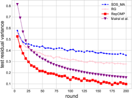
(a) synthetic

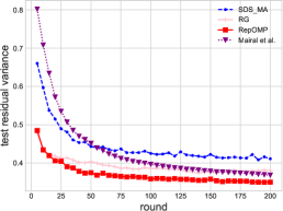
(b) voc

Figure 2: The experimental results for the online setting. In both figures, the horizontal axis indicates the number of rounds. 2(a) is the result with synthetic datasets, and 2(b) is the result with VOC2006 image datasets.

Appendix A Miscellaneous fact

The following folklore result is often useful for proving an approximate ratio.

Lemma A.1.

Suppose that $\Delta_{i},r_{i}\geq 0$ ($i=1,2,\dots$) satisfies

$$\Delta_{i}\geq C\left(v^{*}-\sum_{j=1}^{i-1}\Delta_{j}\right)-r_{i},$$ (6)

for $i=1,2,\dots$, for some constants $C\in[0,1]$ and $v^{*}\geq 0$. Then

$$\sum_{i=1}^{l}\Delta_{i}\geq\left[1-(1-C)^{l}\right]v^{*}-\sum_{i=1}^{l}r_{i}\geq(1-\exp(-Cl))v^{*}-\sum_{i=1}^{l}r_{i}.$$ (7)

for any nonnegative integer $l$.

Proof.

We show

$$v^{*}-\sum_{i=1}^{l}\Delta_{i}\leq\left(1-C\right)^{l}v^{*}+\sum_{i=1}^{l}r_{i}$$ (8)

for $l=0,1,2,\dots$ by the induction on $l$. For $l=0$, (8) is trivial. For $l\geq 1$, we have

$$v^{*}-\sum_{i=1}^{l}\Delta_{i} =v^{*}-\sum_{i=1}^{l-1}\Delta_{i}-\Delta_{l}$$

$$\leq v^{*}-\sum_{i=1}^{l-1}\Delta_{i}-C\left(v^{*}-\sum_{j=1}^{l-1}\Delta_{j}\right)+r_{l}$$

$$=\left(1-C\right)\left(v^{*}-\sum_{i=1}^{l-1}\Delta_{i}\right)+r_{l}.$$

Now (8) follows from the induction and $1-C\in[0,1]$. ∎

Appendix B Missing proofs for generalized sparsity constraints

B.1 Individual matroids

Proposition B.1.

An individual matroid constraint is $k$-replacement sparse.

Proof.

Let $(Z_{1},\cdots,Z_{T}),(Z^{*}_{1},\cdots,Z^{*}_{T})\in\mathcal{I}$ be arbitrary sparse subsets. First we consider the case where $Z_{t}$ and $Z^{*}_{t}$ are both bases of the matroid for all $t\in[T]$. For such $Z_{t}$ and $Z^{*}_{t}$, we can make $k$ replacements as follows: For each $t\in[T]$, there exists a bijection $\pi_{t}\colon Z^{*}_{t}\to Z_{t}$ by the exchange property of matroids. For each atom $a^{*}\in\bigcup_{t=1}^{T}Z^{*}_{t}$, we make a replacement that adds $a^{*}$ to and removes $\pi_{t}(a^{*})$ from $Z_{t}$ for all $t\in[T]$ such that $a^{*}\in Z^{*}_{t}$.

If $Z_{t}$ or $Z^{*}_{t}$ is not a base of the matroid, we can add arbitrary atoms to $Z_{t}$ and $Z^{*}_{t}$ until they are both bases, and make $k$ replacements for them in the same way as described above. Removing the atoms that do not exist in $Z_{t}$ and $Z^{*}_{t}$ from these $k$ replacements, we obtain replacements for original $Z_{t}$ and $Z^{*}_{t}$. ∎

B.2 Block sparsity

Proposition B.2.

A block sparsity constraint is $k$-replacement sparse.

Proof.

Let $(Z_{1},\cdots,Z_{T}),(Z^{*}_{1},\cdots,Z^{*}_{T})\in\mathcal{I}$ be arbitrary sparse subsets. We can make $k$ replacements as follows: Let $Z_{b^{\prime}}=\bigcup_{t\in B_{b^{\prime}}}Z_{t}$ and $Z^{*}_{b^{\prime}}=\bigcup_{t\in B_{b^{\prime}}}Z^{*}_{t}$. If $|Z_{b^{\prime}}|<s_{b^{\prime}}$ or $|Z_{b^{\prime}}|<s_{b^{\prime}}$, we can add arbitrary atoms until these inequalities are tight. For each block $b^{\prime}\in[b]$, we can make a bijection $\pi_{t}\colon Z^{*}_{b}\to Z_{b}$. For each atom $a^{*}\in\bigcup_{t=1}^{T}Z^{*}_{t}$, we make one replacement that adds $a^{*}$ for all $t\in[T]$ such that $a^{*}\in Z^{*}_{t}$ and removes $\pi_{t}(a^{*})$ from all blocks such that $a^{*}\in\bigcup_{t\in B_{b^{\prime}}}Z^{*}_{t}$. ∎

We can show the common generalization of an individual matroid sparsity and block sparsity is also $k$-replacement sparse by combining the proofs.

B.3 Average sparsity without individual sparsity

First we consider an easier case with only a total number constraint, that is, $\mathcal{I}=\{(Z_{1},\cdots,Z_{T})\mid\sum_{t=1}^{T}|Z_{t}|\leq s^{\prime}\}$. We call it an average sparsity constraint without individual sparsity.

Proposition B.3.

An average sparsity constraint without individual sparsity is $(2k-1)$-replacement sparse.

Proof.

Let $(Z_{1},\cdots,Z_{T}),(Z^{*}_{1},\cdots,Z^{*}_{T})\in\mathcal{I}$ be arbitrary feasible sparse subsets. We assume $(Z_{1},\cdots,Z_{T})$ and $(Z^{*}_{1},\cdots,Z^{*}_{T})$ are maximal in $\mathcal{I}$, but we can deal with non-maximal ones by filling them with dummy elements in the same way as the proof of Proposition B.1. Here we show it is possible to greedily make a sequence of $2k-1$ feasible replacements $(Z^{r^{\prime}}_{1},\cdots,Z^{r^{\prime}}_{T})_{r^{\prime}=1}^{2k-1}$ such that each atom in $Z^{*}_{t}\setminus Z_{t}$ appears at least once in the sequence $(Z^{r^{\prime}}_{t}\setminus Z_{t})_{r^{\prime}=1}^{2k-1}$ and each atom in $Z_{t}\setminus Z_{t}^{*}$ appears at most once in the sequence $(Z_{t}\setminus Z^{r^{\prime}}_{t})_{r^{\prime}=1}^{2k-1}$.

Let $X$ and $X^{*}$ be the sets of atoms appearing in $(Z_{1},\cdots,Z_{T})$ and $(Z^{*}_{1},\cdots,Z^{*}_{T})$, respectively. We arrange the atoms in each of $X$ and $X^{*}$ in an arbitrary order and consider them one by one in parallel. Let us suppose we currently consider $a\in X$ and $a^{*}\in X^{*}$. We make a replacement that adds $a^{*}$ for several $t\in[T]$ and removes $a$ for the other several $t\in[T]$ in the following way. Let $\tau$ be the number of $Z_{t}\setminus Z^{*}_{t}$ that contains $a$, i.e., $\tau=|\{t\in[T]\mid a\in Z_{t}\setminus Z^{*}_{t}\}|$ and $\tau^{*}$ the number of $Z^{*}_{t}\setminus Z_{t}$ that contains $a^{*}$, i.e., $\tau=|\{t\in[T]\mid a^{*}\in Z^{*}_{t}\setminus Z_{t}\}|$. If $\tau>\tau^{*}$, we can let this replacement add $a^{*}$ for all $t\in[T]$ such that $a^{*}\in Z^{*}_{t}\setminus Z_{t}$ and remove $a$ for any subset of $\{t\in[T]\mid a\in Z_{t}\setminus Z^{*}_{t}\}$ with size $\tau^{*}$. Conversely, if $\tau\leq\tau^{*}$, we can let this replacement add $a^{*}$ for an arbitrary subset of $\{t\in[T]\mid a^{*}\in Z^{*}_{t}\setminus Z_{t}\}$ of size $\tau$ and remove $a$ for all $t\in[T]$ such that $a\in Z_{t}\setminus Z^{*}_{t}$. We proceed to a next replacement after removing $a^{*}$ from $Z^{*}_{t}$ for all $t\in[T]$ such that $a^{*}$ is added in this replacement, and $a$ from $Z_{t}$ for all $t\in[T]$ such that $a$ is removed in this replacement. If $a\not\in Z_{t}\setminus Z^{*}_{t}$ for all $t\in[T]$, we move the focus from $a$ to the next atom. Similarly, if $a^{*}\not\in Z^{*}_{t}\setminus Z_{t}$ for all $t\in[T]$, we move the focus from $a$ to the next atom.

This procedure ends after at most $2k-1$ iterations. This is because at each iteration we move the focus from $a$ to the next atom in $X$ or from $a^{*}$ to the next atom in $X^{*}$, and we obtain $|X|\leq k$ and $|X^{*}|\leq k$. ∎

Here we show this bound is tight for an average sparsity constraint without individual sparsity by giving an example.

Example B.4.

Assume $T\geq k^{2}$. For simplicity, we further assume $T$ is a multiple of $k$. Let us consider the case of $s^{\prime}=T$, i.e., $\mathcal{I}=\{(Z_{1},\cdots,Z_{T})\mid\sum_{t=1}^{T}|Z_{t}|\leq T\}$. Let $V=\{v_{1},\cdots,v_{2k}\}$ be the ground set. Here we show the replacement sparsity parameter of this sparsity constraint is at least $2k-1$ by giving $(Z_{1},\cdots,Z_{T})$ and $(Z^{*}_{1},\cdots,Z^{*}_{T})$ that require $2k-1$ replacements. Suppose $Z_{t}=\{v_{1},\cdots,v_{k}\}$ for $1\leq t\leq T/k$ and $Z_{t}=\varnothing$ for other $t$. Let $Z^{*}_{t}=\{v_{k+1}\}$ for $1\leq t\leq T-k+1$ and $Z^{*}_{T-k+i}=\{v_{k+i}\}$ for each $i=2,\cdots,k$. .

It can be seen that we must use $k-1$ different replacements for $Z^{*}_{T-k+2},\cdots,Z^{*}_{T}$. In each replacement, an added element is restricted to a single atom, but $Z^{*}_{T-k+2},\cdots,Z^{*}_{T}$ are all singleton sets of different atoms. Then elements in $Z^{*}_{T-k+2},\cdots,Z^{*}_{T}$ must be dealt with by different replacements, and $k-1$ replacements are needed.

In addition, we must use $k$ other replacements for $Z^{*}_{1},\cdots,Z^{*}_{T-k+1}$. Since $(Z_{1},\cdots,Z_{T})$ is maximal in $\mathcal{I}$, the total number of added atoms of each replacement must be at most the total number of removed atoms of this replacement. However, in each replacement, the number of atoms removed from each $Z_{t}$ is at most one, and only $Z_{1},\cdots,Z_{T/k}$ are non-empty, hence at most $T/k$ elements can be removed in each replacement. Therefore, we must use $k$ different replacements for $Z^{*}_{1},\cdots,Z^{*}_{T-k+1}$ because there are $T-k+1$ singleton sets $Z^{*}_{1},\cdots,Z^{*}_{T-k+1}$ and $T\geq k^{2}$.

In conclusion, the replacement sparsity parameter of this sparsity constraint is at least $2k-1$.

B.4 Average sparsity

We bound the replacement sparsity parameter of an average sparsity constraint based on the analysis on average sparsity without individual sparsity.

Proposition B.5.

An average sparsity constraint is $(3k-1)$-replacement sparse.

Proof.

Here we give a sequence of $3k-1$ replacements that satisfies the conditions for replacement sparsity.

First we use $k$ replacements for dealing with the individual sparsity constraints. Let $S\subseteq[T]$ be the set of indices such that $|Z_{t}|=s_{t}$. For each $a^{*}\in X^{*}$, we make a replacement that adds $a^{*}$ for all $t\in S$ such that $a^{*}\in Z^{*}_{t}\setminus Z_{t}$ and possibly removes an atom in $Z_{t}\setminus Z^{*}_{t}$ for all $t\in S$. By selecting the removed atoms so that they do not overlap, we can define these $k$ replacements such that, for all $t\in S$, each atom in $Z^{*}_{t}\setminus Z_{t}$ is added once and each atom in $Z_{t}\setminus Z^{*}_{t}$ is removed once.

For the rest of the elements, we need not consider the individual sparsity constraints, therefore the rest elements can be dealt with $2k-1$ replacements in the same way as the proof of Proposition B.3. ∎

Appendix C Proofs for Replacement Greedy and Replacement OMP

C.1 Proof for Replacement Greedy

Lemma C.1.

Assume $\mathcal{I}$ is $p$-replacement sparse. Suppose that at some step, the solution is updated from $(Z_{1},\cdots,Z_{T})$ to $(Z^{\prime}_{1},\cdots,Z^{\prime}_{T})$ by Replacement Greedy. Let $(Z^{*}_{1},\cdots,Z^{*}_{T})\in\operatorname*{argmax}_{(Z_{1},\cdots,Z_{T})\in\mathcal{I}\colon Z_{t}\subseteq X^{*}}f_{t}(Z)$ where $X^{*}$ is an optimal solution for dictionary selection. Then, the marginal gain of Replacement Greedy is bounded from below as follows:

$$\sum_{t=1}^{T}f_{t}(Z^{\prime}_{t})-\sum_{t=1}^{T}f_{t}(Z_{t})\geq\frac{1}{p}\left\{\frac{m_{2s}}{M_{s,2}}\sum_{t=1}^{T}f_{t}(Z^{*}_{t})-\frac{M_{s,2}}{m_{2s}}\sum_{t=1}^{T}f_{t}(Z_{t})\right\}$$

where $s=\max_{(Z_{t})_{t=1}^{T}\in\mathcal{I}}\max_{t\in[T]}|Z_{t}|$.

Proof.

Note that from the condition on feasible replacements, we have $|Z_{t}\triangle Z^{\prime}_{t}|\leq 2$. Since $u_{t}$ is $M_{s,2}$-smooth on $\Omega_{s,2}$, it holds that for any $\mathbf{z}\in\mathbb{R}^{n}$ with $\mathrm{supp}(\mathbf{z})\subseteq Z^{\prime}_{t}\setminus Z_{t}$,

$$f_{t}(Z^{\prime}_{t})-f_{t}(Z_{t}) =u_{t}(\mathbf{w}^{(Z^{\prime}_{t})})-u_{t}(\mathbf{w}^{(Z_{t})})$$

$$\geq u_{t}((\mathbf{w}^{(Z_{t})})_{Z_{t}\cap Z^{\prime}_{t}}+\mathbf{z})-u_{t}(\mathbf{w}^{(Z_{t})})$$

$$\geq\left\langle\nabla u_{t}(\mathbf{w}^{(Z_{t})}),\mathbf{z}-(\mathbf{w}^{(Z_{t})})_{Z_{t}\setminus Z^{\prime}_{t}}\right\rangle-\frac{M_{s,2}}{2}\lVert\mathbf{z}-(\mathbf{w}^{(Z_{t})})_{Z_{t}\setminus Z^{\prime}_{t}}\rVert^{2}$$

Since this inequality holds for every $\mathbf{z}$ with $\mathrm{supp}(\mathbf{z})\subseteq Z^{\prime}_{t}\setminus Z_{t}$, by optimizing it for $\mathbf{z}$, we obtain

$$f_{t}(Z^{\prime}_{t})-f_{t}(Z_{t})\geq\frac{1}{2M_{s,2}}\lVert\nabla u_{t}(\mathbf{w}_{t}^{(Z_{t})})_{Z^{\prime}_{t}\setminus Z_{t}}\rVert^{2}-\frac{M_{s,2}}{2}\lVert(\mathbf{w}_{t}^{(Z_{t})})_{Z_{t}\setminus Z^{\prime}_{t}}\rVert^{2}.$$ (9)

In addition, due to the strong concavity of $u_{t}$, we have

$$f_{t}(Z_{t}^{*})-f_{t}(Z_{t}) =u_{t}(\mathbf{w}^{(Z_{t}^{*})})-u_{t}(\mathbf{w}^{(Z_{t})})$$

$$\leq\left\langle\nabla u_{t}(\mathbf{w}_{t}^{(Z_{t})}),\mathbf{w}_{t}^{(Z^{*}_{t})}-\mathbf{w}_{t}^{(Z_{t})}\right\rangle-\frac{m_{2s}}{2}\left\|\mathbf{w}_{t}^{(Z_{t}^{*})}-\mathbf{w}_{t}^{(Z_{t})}\right\|^{2}$$

$$\leq\max_{\mathbf{z}\colon\mathrm{supp}(\mathbf{z})\subseteq Z_{t}^{*}}\left\{\left\langle\nabla u_{t}(\mathbf{w}_{t}^{(Z_{t})}),\mathbf{z}-\mathbf{w}_{t}^{(Z_{t})}\right\rangle-\frac{m_{2s}}{2}\left\|\mathbf{z}-\mathbf{w}_{t}^{(Z_{t})}\right\|^{2}\right\}$$

$$=\frac{1}{2m_{2s}}\left\|(\nabla u_{t}(\mathbf{w}^{(Z_{t})}))_{Z_{t}^{*}\setminus Z_{t}}\right\|^{2}-\frac{m_{2s}}{2}\left\|(\mathbf{w}^{(Z_{t})})_{Z_{t}\setminus Z_{t}^{*}}\right\|^{2}.$$ (10)

Similarly, due to the strong concavity of $u_{t}$, we have

$$-f_{t}(Z_{t}) =u_{t}(\mathbf{0})-u_{t}(\mathbf{w}_{t}^{(Z_{t})})$$

$$\leq\left\langle\nabla u_{t}(\mathbf{w}_{t}^{(Z_{t})}),-\mathbf{w}_{t}^{(Z_{t})}\right\rangle-\frac{m_{2s}}{2}\left\|\mathbf{w}_{t}^{(Z_{t})}\right\|^{2}$$

$$=-\frac{m_{2s}}{2}\left\|\mathbf{w}_{t}^{(Z_{t})}\right\|^{2}$$

$$\leq-\frac{m_{2s}}{2}\left\|(\mathbf{w}_{t}^{(Z_{t})})_{Z_{t}\setminus Z^{*}_{t}}\right\|^{2}$$ (11)

Since $\mathcal{I}$ is $p$-replacement sparse, we can take a sequence of $p$ replacements $(Z^{p^{\prime}}_{1},\cdots,Z^{p^{\prime}}_{T})_{p^{\prime}=1}^{p}$ such that

• $(Z^{p^{\prime}}_{1},\cdots,Z^{p^{\prime}}_{T})\in\mathcal{F}(Z_{1},\cdots,Z_{T})$,

• each element in $Z^{*}_{t}\setminus Z_{t}$ appears at least once in sequence $(Z^{p^{\prime}}_{t}\setminus Z_{t})_{p^{\prime}=1}^{p}$ for each $t\in[T]$,

• each element in $Z_{t}\setminus Z_{t}^{*}$ appears at most once in sequence $(Z_{t}\setminus Z^{p^{\prime}}_{t})_{p^{\prime}=1}^{p}$ for each $t\in[T]$.

Now we prove the lemma by utilizing these properties.

$$\sum_{t=1}^{T}f_{t}(Z^{\prime}_{t})-\sum_{t=1}^{T}f_{t}(Z_{t})$$

$$\geq\frac{1}{p}\sum_{p^{\prime}=1}^{p}\left\{\sum_{t=1}^{T}f_{t}(Z^{p^{\prime}}_{t})-\sum_{t=1}^{T}f_{t}(Z_{t})\right\} (Z_{1}^{\prime},\dots,Z_{T}^{\prime}) (Z^{p^{\prime}}_{1},\cdots,Z^{p^{\prime}}_{T})$$ (by the choice of and the feasibility of )

$$\geq\frac{1}{p}\sum_{p^{\prime}=1}^{p}\sum_{t=1}^{T}\left\{\frac{1}{2M_{s,2}}\left\lVert\nabla u_{t}(\mathbf{w}_{t}^{(Z_{t})})_{Z^{p^{\prime}}_{t}\setminus Z_{t}}\right\rVert^{2}-\frac{M_{s,2}}{2}\left\lVert\left(\mathbf{w}_{t}^{(Z_{t})}\right)_{Z_{t}\setminus Z^{p^{\prime}}_{t}}\right\rVert^{2}\right\}$$ (by (9))

$$\geq\frac{1}{p}\sum_{t=1}^{T}\left\{\frac{1}{2M_{s,2}}\left\lVert\nabla u_{t}(\mathbf{w}_{t}^{(Z_{t})})_{Z^{*}_{t}\setminus Z_{t}}\right\rVert^{2}-\frac{M_{s,2}}{2}\left\lVert\left(\mathbf{w}_{t}^{(Z_{t})}\right)_{Z_{t}\setminus Z_{t}^{*}}\right\rVert^{2}\right\} (Z_{t}^{p^{\prime}})_{p^{\prime}=1}^{p}$$ (by the property of )

$$\geq\frac{1}{p}\sum_{t=1}^{T}\left\{\frac{m_{2s}}{M_{s,2}}\left(f_{t}(Z_{t}^{*})-f_{t}(Z_{t})\right)-\left(\frac{M_{s,2}}{m_{2s}}-\frac{m_{2s}}{M_{s,2}}\right)f_{t}(Z_{t})\right\}$$ (by (C.1) and (C.1))

$$=\frac{1}{p}\sum_{t=1}^{T}\left\{\frac{m_{2s}}{M_{s,2}}f_{t}(Z_{t}^{*})-\frac{M_{s,2}}{m_{2s}}f_{t}(Z_{t})\right\}.$$

∎

Combined with Lemma A.1, Theorem 4.1 is obtained.

C.2 Proof for Replacement OMP

Lemma C.2.

Assume $\mathcal{I}$ is $p$-replacement sparse. Suppose at some step, the solution is updated from $(Z_{1},\cdots,Z_{T})$ to $(Z^{\prime}_{1},\cdots,Z^{\prime}_{T})$ by Replacement OMP. Let $(Z^{*}_{1},\cdots,Z^{*}_{T})\in\operatorname*{argmax}_{(Z_{1},\cdots,Z_{T})\in\mathcal{I}\colon Z_{t}\subseteq X^{*}}f_{t}(Z)$ where $X^{*}$ is an optimal solution for dictionary selection. Then, the marginal gain of Replacement OMP is bounded from below as follows:

$$\sum_{t=1}^{T}f_{t}(Z^{\prime}_{t})-\sum_{t=1}^{T}f_{t}(Z_{t})\geq\frac{1}{p}\left\{\frac{m_{2s}}{M_{s,2}}\sum_{t=1}^{T}f_{t}(Z^{*}_{t})-\frac{M_{s,2}}{m_{2s}}\sum_{t=1}^{T}f_{t}(Z_{t})\right\}$$

where $s=\max_{(Z_{t})_{t=1}^{T}\in\mathcal{I}}\max_{t\in[T]}|Z_{t}|$.

Proof.

We can obtain the following inequalities from the strong concavity and smoothness of $u_{t}$ in the same way as the above proof of Lemma C.1.

$$f_{t}(Z^{\prime}_{t})-f_{t}(Z_{t}) \geq\frac{1}{2M_{s,2}}\left\lVert\nabla u_{t}(\mathbf{w}_{t}^{(Z_{t})})_{Z^{\prime}_{t}\setminus Z_{t}}\right\rVert^{2}-\frac{M_{s,2}}{2}\left\lVert(\mathbf{w}_{t}^{(Z_{t})})_{Z_{t}\setminus Z^{\prime}_{t}}\right\rVert^{2}.$$ (12)

$$f_{t}(Z_{t}^{*})-f_{t}(Z_{t}) \leq\frac{1}{2m_{2s}}\left\|(\nabla u_{t}(\mathbf{w}^{(Z_{t})}))_{Z_{t}^{*}\setminus Z_{t}}\right\|^{2}-\frac{m_{2s}}{2}\left\|(\mathbf{w}^{(Z_{t})})_{Z_{t}\setminus Z_{t}^{*}}\right\|^{2}.$$ (13)

$$-f_{t}(Z_{t}) \leq-\frac{m_{2s}}{2}\left\|(\mathbf{w}_{t}^{(Z_{t})})_{Z_{t}\setminus Z^{*}_{t}}\right\|^{2}.$$ (14)

Since $\mathcal{I}$ is $p$-replacement sparse, we can take a sequence of $p$ replacements $(Z^{p^{\prime}}_{1},\cdots,Z^{p^{\prime}}_{T})_{p^{\prime}=1}^{p}$ that satisfies the properties mentioned in the proof of Lemma C.1. With these properties, we obtain

$$\sum_{t=1}^{T}f_{t}(Z^{\prime}_{t})-\sum_{t=1}^{T}f_{t}(Z_{t})$$

$$\geq\sum_{t=1}^{T}\left\{\frac{1}{2M_{s,2}}\left\lVert\nabla u_{t}(\mathbf{w}_{t}^{(Z_{t})})_{Z^{\prime}_{t}\setminus Z_{t}}\right\rVert^{2}-\frac{M_{s,2}}{2}\left\lVert(\mathbf{w}_{t}^{(Z_{t})})_{Z_{t}\setminus Z^{\prime}_{t}}\right\rVert^{2}\right\}$$ (by (12))

$$\geq\frac{1}{p}\sum_{p^{\prime}=1}^{p}\sum_{t=1}^{T}\left\{\frac{1}{2M_{s,2}}\left\lVert\nabla u_{t}(\mathbf{w}_{t}^{(Z_{t})})_{Z^{p^{\prime}}_{t}\setminus Z_{t}}\right\rVert^{2}-\frac{M_{s,2}}{2}\left\lVert\left(\mathbf{w}_{t}^{(Z_{t})}\right)_{Z_{t}\setminus Z^{p^{\prime}}_{t}}\right\rVert^{2}\right\} (Z_{1}^{\prime},\dots,Z_{T}^{\prime}) (Z^{p^{\prime}}_{1},\cdots,Z^{p^{\prime}}_{T})$$ (by the choice of and the feasibility of )

$$\geq\frac{1}{p}\sum_{t=1}^{T}\left\{\frac{1}{2M_{s,2}}\left\lVert\nabla u_{t}(\mathbf{w}_{t}^{(Z_{t})})_{Z^{*}_{t}\setminus Z_{t}}\right\rVert^{2}-\frac{M_{s,2}}{2}\left\lVert\left(\mathbf{w}_{t}^{(Z_{t})}\right)_{Z_{t}\setminus Z_{t}^{*}}\right\rVert^{2}\right\} (Z_{t}^{p^{\prime}})_{p^{\prime}=1}^{p}$$ (by the property of )

$$\geq\frac{1}{p}\sum_{t=1}^{T}\left\{\frac{m_{2s}}{M_{s,2}}\left(f_{t}(Z_{t}^{*})-f_{t}(Z_{t})\right)-\left(\frac{M_{s,2}}{m_{2s}}-\frac{m_{2s}}{M_{s,2}}\right)f_{t}(Z_{t})\right\}$$ (by (13) and (14))

$$=\frac{1}{p}\sum_{t=1}^{T}\left\{\frac{m_{2s}}{M_{s,2}}f_{t}(Z_{t}^{*})-\frac{M_{s,2}}{m_{2s}}f_{t}(Z_{t})\right\}.$$

∎

Combined with Lemma A.1, we obtain Theorem 4.2.

C.2.1 About greedy selection at each step

Next we consider how to find the atom with the largest gain at each step of Replacement OMP for the average sparsity constraints.

First we show that this task reduces to weighted bipartite matching. Let us fix an atom $a^{*}$ because we can simply check all the atoms in $V$. Let $g_{t}=(\nabla u_{t}(\mathbf{w}^{(Z_{t})}))^{2}_{a^{*}}$ and $c_{t}=\min_{a\in Z_{t}}(\mathbf{w}^{(Z_{t})})^{2}_{a}$ for each $t\in[T]$. Let $S=\{t\in[T]\mid|Z_{t}|=s_{t}\}$ be the set of $t\in[T]$ such that the constraint on $|Z_{t}|$ is tight.

For each $a^{*}\in V$, the problem of finding the best replacement can be formulated as follows: The goal is to maximize $\sum_{t\in A}g_{t}-\sum_{t\in B}c_{t}$ by selecting $A\subseteq[T]$ (the set of indices $t$ such that $a^{*}$ is added to $Z_{t}$) and $B\subseteq[T]$ (the set of indices $t$ such that an atom is removed from $Z_{t}$). We have two constraints on $A$ and $B$. The first constraint is $|A|-|B|\leq\theta$ where $\theta=s^{\prime}-\sum_{t=1}^{T}|Z_{t}|$, derived from the total number constraint $\sum_{t=1}^{T}|Z_{t}|$. The second constraint is $A\cap S\subseteq B$, derived from the individual constraint $|Z_{t}|\leq s_{t}$. In summary, the formulation as an optimization problem is:

$$\max_{A,B\subseteq[T]}\quad \sum_{t\in A}g_{t}-\sum_{t\in B}c_{t}$$

subject to $$|A|-|B|\leq\theta$$

$$A\cap S\subseteq B.$$

This problem can be regarded as a special case of maximum weight bipartite matching problem. Let $U=[T]$ and $V=[T]\cup\{d_{1},\cdots,d_{\theta}\}$ be the set of vertices where $d_{1},\cdots,d_{\theta}$ are dummy elements with zero cost, i.e., $c_{d_{i}}=0$ for all $i\in[\theta]$. Let $E=\{(t,t)\mid t\in S\}\cup(U\setminus S)\times V$ be the set of edges. The weight of each edge $(\alpha,\beta)\in E$ is defined as $w((\alpha,\beta))=g_{\alpha}-c_{\beta}$. Then any matching $M\subseteq E$ in this graph corresponds to a solution $A=\partial M\cap U$ and $B=\partial M\cap V\setminus\{d_{1},\cdots,d_{\theta}\}$ in the above optimization problem.

Algorithm 2 Calculation of the gain for average sparsity constraints

0:  $S=\{t\in[T]\mid|Z_{t}|=s_{t}\}$ the set of indices $t$ such that $Z_{t}$ is tight, $g_{t}=(\nabla u_{t}(\mathbf{w}^{(Z_{t})}))^{2}_{a^{*}}$, $c_{t}=\min_{a\in Z_{t}}(\mathbf{w}^{(Z_{t})})^{2}_{a}$ for each $t\in[T]$, and $\theta=s^{\prime}-\sum_{t=1}^{T}|Z_{t}|$.

0:  $A,B\subseteq[T]$ maximizing $\sum_{t\in A}g_{t}-\sum_{t\in B}c_{t}$ subject to $A\cap S\subseteq B$ and $|A|\leq|B|+\theta$.

1:  Initialize $A_{0}\leftarrow\varnothing$ and $B_{0}\leftarrow\varnothing$.

2:  Let $S=\{t\in[T]\mid|Z_{t}|=s_{t}\}$.

3:  Sort $t\in[T]\setminus S$ according to $g_{t}$ into the priority queue $Q_{1}$ in descending order.

4:  Sort $t\in[T]$ according to $c_{t}$ into the priority queue $Q_{2}$ in ascending order.

5:  Sort $t\in S$ according to $g_{t}-c_{t}$ into the priority queue $Q_{3}$ in descending order.

6:  for $i=1,\cdots,T$ do

7:     Let $\alpha$, $\beta$ and $\gamma$ be the top elements in $Q_{1}$, $Q_{2}$, and $Q_{3}$, respectively.

8:     if $g_{\alpha}-c_{\beta}\mathbf{1}\{|A_{i-1}|=|B_{i-1}|+\theta\}\leq 0$ and $g_{\gamma}-c_{\gamma}\leq 0$ then

9:        return $A_{i-1}$ and $B_{i-1}$

10:     else

11:        if $g_{\alpha}-c_{\beta}\mathbf{1}\{|A_{i-1}|=|B_{i-1}|+\theta\}\geq g_{\gamma}-c_{\gamma}$ then

12:           $A_{i}\leftarrow A_{i-1}+\alpha$ and remove $\alpha$ from $Q_{1}$.

13:           if $|A_{i-1}|=|B_{i-1}|+\theta$ then

14:              $B_{i}\leftarrow B_{i-1}+\beta$ and remove $\beta$ from $Q_{2}$.

15:              if $\beta\in S$ then

16:                 Remove $\beta$ from $Q_{3}$ and add $\beta$ to $Q_{1}$.

17:        else

18:           $A_{i}\leftarrow A_{i-1}+\gamma$ and $B_{i}\leftarrow B_{i-1}+\gamma$.

19:           Remove $\gamma$ from $Q_{3}$.

20:  return $A_{T}$ and $B_{T}$

Here we give a fast greedy method for calculating the gain of each atom. This algorithm can be executed in $\mathrm{O}(T\log T)$ time. The detailed description of this algorithm is given in Algorithm 2.

Proposition C.3.

Algorithm 2 returns an optimal solution in $\mathrm{O}(T\log T)$ time.

Proof.

First we show the validity of the algorithm.

Before proving the optimality of the output, we note that the marginal gain of each step of the algorithm is largest among all the feasible updates. Let us consider the addition of $\alpha$ to $A_{i-1}$. There are three cases of updates. If $\alpha\in S\setminus B_{i-1}$ is added to $A_{i-1}$, we must also add $\alpha$ to $B_{i-1}$. If $\alpha\not\in S\setminus B_{i-1}$ and $|A_{i-1}|=|B_{i-1}|+\theta$, adding $\beta\not\in B_{i-1}$ with smallest cost $c_{t}$ is the best choice. If $\alpha\not\in S\setminus B_{i-1}$ and $|A_{i-1}|<|B_{i-1}|+\theta$, not changing $B_{i-1}$ is the best choice. Algorithm 2 selects the best one from these cases.

We show $(A_{i},B_{i})$ be optimal among feasible solutions such that $|A|=i$ by induction on $i$. It is clear that $(A_{0},B_{0})$ is optimal among feasible solutions such that $|A|=0$.

Now we assume $(A_{i-1},B_{i-1})$ is optimal among feasible solutions such that $|A|=i-1$. Let $(A^{\prime}_{i},B^{\prime}_{i})$ be an optimal solution among feasible solutions such that $|A|=i$. If there exist $\alpha\in A^{\prime}_{i}\setminus A_{i-1}$ and $\beta\in B^{\prime}_{i}\setminus B_{i-1}$ such that $(A_{i-1}+\alpha,B_{i-1}+\beta)$ and $(A^{\prime}_{i}-\alpha,B^{\prime}_{i}-\beta)$ are both feasible, we obtain

$$\sum_{t\in A_{i}}g_{t}-\sum_{t\in B_{i}}c_{t} \geq\left(\sum_{t\in A_{i-1}}g_{t}-\sum_{t\in B_{i-1}}c_{t}\right)+\left(g_{\alpha_{i}}-c_{\beta_{i}}\right)$$

$$\geq\left(\sum_{t\in A^{\prime}_{i-1}}g_{t}-\sum_{t\in B^{\prime}_{i-1}}c_{t}\right)+\left(g_{\alpha^{\prime}}-c_{\beta^{\prime}}\right)$$

$$\geq\left(\sum_{t\in A^{\prime}_{i}}g_{t}-\sum_{t\in B^{\prime}_{i}}c_{t}\right),$$

which proves the optimality of $(A_{i},B_{i})$. The second inequality is because the marginal gain of $\alpha_{i}$ (or possibly $\alpha_{i}$ and $\beta_{i}$) is largest among feasible additions. In the same way, if there exist $\alpha\in A^{\prime}_{i}\setminus A_{i-1}$ such that $(A_{i-1}+\alpha,B_{i-1})$ and $(A^{\prime}_{i}-\alpha,B^{\prime}_{i})$ are both feasible, then $(A_{i},B_{i})$ is optimal.

We show the existence of such an $\alpha$ or pair $(\alpha,\beta)$. Since $|A^{\prime}_{i}|>|A_{i-1}|$, we have $A^{\prime}_{i}\setminus A_{i-1}\neq\varnothing$. Let $\alpha\in A^{\prime}_{i}\setminus A_{i-1}$ be an arbitrary element. If $\alpha\in B^{\prime}_{i}\setminus B_{i-1}$, the pair $(\alpha,\alpha)$ satisfies the condition. If $\alpha\not\in B^{\prime}_{i}\setminus B_{i-1}$ and $|A_{i-1}|<|B_{i-1}|+\theta$, then $\alpha$ satisfies the condition. If $\alpha\not\in B^{\prime}_{i}\setminus B_{i-1}$ and $|A_{i-1}|=|B_{i-1}|+\theta$, we have $|B^{\prime}_{i}|\geq|A^{\prime}_{i}|-\theta>|B_{i-1}|$, then $B^{\prime}_{i}\setminus B_{i-1}\neq\varnothing$. Therefore a pair of $\alpha$ and an arbitrary $\beta\in B^{\prime}_{i}\setminus B_{i-1}$ satisfies the condition.

Finally we consider the running time of this algorithm. Sorting requires $\mathrm{O}(T\log T)$ time. Each iteration requires $\mathrm{O}(\log T)$ time. Thus, the total running time is $\mathrm{O}(T\log T)$. ∎

C.3 Proof of Theorem 4.3

Proof.

In each iteration, we need to find an atom with the largest gain and the corresponding new supports $(Z_{1}^{\prime},\dots,Z_{t}^{\prime})$. This can be done in $\mathrm{O}(nT\log T)$ time. Furthermore, we need to compute a new coefficient $\mathbf{w}^{(Z^{\prime}_{t})}_{t}=\mathbf{A}_{{Z^{\prime}_{t}}}^{+}\mathbf{y}_{t}$ for the new support ${Z^{\prime}_{t}}$ ($t\in[T]$), where $\mathbf{A}^{+}$ is the pseudo inverse. This can be done efficiently via maintaining the QR-decomposition of $\mathbf{A}_{Z_{t}}$ under rank-two update [18] with a cost of $\mathrm{O}(s^{2}+ds)=\mathrm{O}(ds)$ time for each matrix. Thus each iteration requires $\mathrm{O}(T(n\log T+ds))$ time, which proves the theorem. ∎

Appendix D Online dictionary selection

Online dictionary selection is the problem of selecting a dictionary at each round. At each round $t$, the player selects a dictionary $X_{t}\subseteq V$ with $|X_{t}|\leq k$, then the adversary reveals a data point $\mathbf{y}_{t}\in\mathbb{R}^{d}$. Then the player gains with respect to the best $s$-sparse approximation to $\mathbf{y}_{t}$ with the selected dictionary $X_{t}$:

$$\max_{\mathbf{w}\colon\lVert\mathbf{w}\rVert_{0}\leq s}u(\mathbf{y}_{t},\mathbf{A}_{X_{t}}\mathbf{w}),$$ (15)

where $\mathbf{A}_{X_{t}}$ is the matrix obtained by arranging all vectors contained in $X_{t}$. Let $g_{t}(X)=\max_{Z\subseteq X\colon|Z|\leq s}f_{t}(Z)$ be the objective function at the $t$th round, where $f_{t}(Z)=\max_{\mathbf{w}\colon\lVert\mathbf{w}\rVert_{0}\leq s}u(\mathbf{y}_{t},A_{Z}\mathbf{w})$. In the following, we provide the online versions of algorithms for offline dictionary selection: Online $\textsf{SDS}_{\textsf{MA}}$, Online Replacement Greedy, and Online Replacement OMP.

D.1 Online $\textsf{SDS}_{\textsf{MA}}$

The first algorithm is based on $\textsf{SDS}_{\textsf{MA}}$ for offline dictionary selection, which was proposed by Krause and Cevher [22] and given an improved analysis by Das and Kempe [10]. At each round $t$, we consider a function $\tilde{f}_{t}(Z)=\sum_{a\in Z}f_{t}(a|\varnothing)$, which is a modular approximation of $f_{t}$. Intuitively, the modular approximation $\tilde{f}_{t}$ ignores the interactions among the atoms. We define the surrogate objective $\tilde{g}_{t}$ as

$$\tilde{g}_{t}(X)=\max_{Z\subseteq X\colon|Z|\leq s}\tilde{f}_{t}(Z).$$ (16)

It is easy to show that $\tilde{g}_{t}$ is monotone submodular. Hence, we can apply the online greedy algorithm [31] to these surrogate functions.

Let $u_{t}(\mathbf{w})\coloneqq u(\mathbf{y}_{t},\mathbf{A}\mathbf{w})$ for $t\in[T]$. Assuming the strong concavity and smoothness of $u_{t}$, the original objective function $g_{t}$ can be bounded from lower and upper with the surrogate function $\tilde{g}_{t}$. A similar result is given in Elenberg et al. [13] for offline sparse regression.

Lemma D.1.

Suppose $u_{t}$ is $m_{1}$-strongly concave and $M_{1}$-smooth on $\Omega_{1}$, and $m_{s}$-strongly concave and $M_{s}$-smooth on $\Omega_{s}$. Then,

$$\frac{m_{1}}{M_{s}}\tilde{g}_{t}(X)\leq g_{t}(X)\leq\frac{M_{1}}{m_{s}}\tilde{g}_{t}(X).$$

Proof.

Let $Z\subseteq V$ be an arbitrary subset such that $|Z|\leq s$. Since the submodularity ratio $\gamma_{\varnothing,s}$ of $f$ is no less than $m_{s}/M_{1}$ [13],

$$\frac{m_{s}}{M_{1}}f_{t}(Z)\leq\sum_{a\in Z}\tilde{f}_{t}(a)=\tilde{f}_{t}(Z).$$

As this bound holds for any $Z\subseteq V$ of size no more than $s$, we have

$$g_{t}(X)=\max_{Z\subseteq X\colon|Z|\leq s}f_{t}(Z)\leq\frac{M_{1}}{m_{s}}\max_{Z\subseteq X\colon|Z|\leq s}\tilde{f}_{t}(Z)=\frac{M_{1}}{m_{s}}\tilde{g}_{t}(X).$$

Next we prove the lower bound of $g_{t}(X)$. From the optimality of $\mathbf{w}^{(Z)}$, for any $\mathbf{z}$ such that $\mathrm{supp}(\mathbf{z})\subseteq Z$,

$$f_{t}(Z) =u_{t}(\mathbf{w}^{(Z)})-u_{t}(\mathbf{0})$$

$$\geq u_{t}(\mathbf{z})-u_{t}(\mathbf{0})$$

$$\geq\langle\nabla u_{t}(\mathbf{0}),\mathbf{z}\rangle-\frac{M_{s}}{2}\|\mathbf{z}\|^{2}$$

where the last inequality is due to the strong concavity of $u_{t}$. Using $\mathbf{z}=\frac{1}{M_{s}}(\nabla u_{t}(\mathbf{0}))_{Z}$, we obtain

$$f_{t}(Z)\geq\frac{1}{2M_{s}}\|(\nabla u_{t}(\mathbf{0}))_{Z}\|^{2}.$$ (17)

On the other hand, from the smoothness of $u_{t}$, we have for all $a\in Z$,

$$f_{t}(a) =u_{t}(\mathbf{w}^{(a)})-u_{t}(\mathbf{0})$$

$$\leq\langle\nabla u_{t}(\mathbf{0}),\mathbf{w}^{(a)}\rangle-\frac{m_{1}}{2}\|\mathbf{w}^{(a)}\|^{2}$$

$$\leq\max_{c\in\mathbb{R}}\langle\nabla u_{t}(\mathbf{0}),c\mathbf{e}_{a}\rangle-\frac{m_{1}}{2}\|c\mathbf{e}_{a}\|^{2}$$

$$=\frac{1}{2m_{1}}(\nabla u_{t}(\mathbf{0}))_{a}^{2}.$$

Summing up for all $a\in Z$, we obtain

$$\tilde{f}_{t}(Z)=\sum_{a\in Z}f_{t}(a)\leq\frac{1}{2m_{1}}\|(\nabla u_{t}(\mathbf{0}))_{Z}\|^{2}.$$ (18)

Combining (17) and (18), we obtain the lower bound

$$f_{t}(Z)\geq\frac{m_{1}}{M_{s}}\tilde{f}_{t}(Z),$$

which proves the lower bound of $g_{t}(X)$ in the same way as the upper bound. ∎

The expected regret of this algorithm can be bounded as follows.

Theorem D.2.

Let $\alpha=(1-\frac{1}{\mathrm{e}})\frac{m_{1}m_{s}}{M_{1}M_{s}}$. The expected $\alpha$-regret of the modular approximation algorithm after $T$ rounds is bounded as follows:

$$\operatorname{regret}_{\alpha}(T)\leq\frac{k\Delta_{\max}m_{1}}{M_{s}}\sqrt{2T\ln n}$$

where $n=|V|$ and $\Delta_{\max}=\max_{a\in V}\max_{t\in[T]}f_{t}(a|\varnothing)$.

Proof.

Applying the regret bound for online submodular maximization [31], we obtain

$$\left(1-\frac{1}{\mathrm{e}}\right)\sum_{t=1}^{T}\tilde{g}_{t}(X^{*})-\sum_{t=1}^{T}\tilde{g}_{t}(X_{t})\leq k\Delta_{\max}\sqrt{2T\ln n}.$$ (19)

since the gains for each subroutine are bounded by $\Delta_{\max}$. From Lemma D.1, we obtain the bound in the statement. ∎

For the squared $\ell^{2}$-utility function $u(\mathbf{y},\mathbf{x})=\frac{1}{2}\lVert\mathbf{y}\rVert_{2}^{2}-\frac{1}{2}\lVert\mathbf{y}-\mathbf{x}\rVert_{2}^{2}$, $\alpha$ is equal to an approximation ratio shown in Das and Kempe [10].

Corollary D.3.

For the squared $\ell^{2}$-utility function, the expected regret of the modular approximation algorithm is

$$\operatorname{regret}_{\alpha}(T)\leq\frac{k\Delta_{\max}}{\sigma_{\mathrm{max}}^{2}(\mathbf{A},s)}\sqrt{2T\ln n},$$

where $\alpha=(1-\frac{1}{\mathrm{e}})\frac{\sigma_{\mathrm{min}}^{2}(\mathbf{A},s)}{\sigma_{\mathrm{max}}^{2}(\mathbf{A},s)}$.

D.2 Online Replacement Greedy

In the following, we provide online adoptation of Replacement Greedy. Similarly to Streeter and Golovin [31], we use $k$ expert algorithms $\mathcal{A}^{1},\cdots,\mathcal{A}^{k}$ as subroutines. At each round, online Replacement Greedy selects a set of $k$ elements $a_{t}^{1},\cdots,a_{t}^{k}$ according to the expert algorithms $\mathcal{A}^{1},\cdots,\mathcal{A}^{k}$, respectively. After the target point $\mathbf{y}_{t}$ is revealed, the algorithm decides the feedback to the subroutines by considering how $Z_{t}$ changes if $a_{t}^{1},\cdots,a_{t}^{k}$ are added to $X$ sequentially. As in the offline version of Replacement Greedy, we start with $Z_{t}^{0}=\varnothing$ and consider adding $a_{t}^{i}$ to $Z_{t}$ or not with keeping $|Z_{t}|\leq s$ for each $i=1,\cdots,k$. Denoting $Z_{t}$ at the $i$th step by $Z_{t}^{i}$, we can write the feedback given to the subroutine $\mathcal{A}^{i}$ as $\Delta_{t}(\cdot,Z_{t}^{i-1})$ where

$$\Delta_{t}(a,Z_{t}^{i})=\begin{cases}\displaystyle f_{t}(Z_{t}^{i}+a)-f_{t}(Z_{t}^{i})&(i<s)\\ \displaystyle\max\left\{0,\max_{a^{\prime}\in Z_{t}^{i}}\left\{f_{t}(Z_{t}^{i}-a^{\prime}+a)-f_{t}(Z_{t}^{i})\right\}\right\}&(i\geq s)\end{cases}$$

is the gain obtained by adding $a$ to $Z_{t}^{i}$. If $\Delta_{t}(a^{i}_{t},Z_{t}^{i-1})>0$, the algorithm updates $Z_{t}$ by adding $a_{t}^{i}$ and, if $i>s$, removing $a^{\prime}$ that maximizing $f_{t}(Z_{t}^{i-1}-a^{\prime}+a_{t}^{i})$. For each $a\in V$, the value of gain $\Delta_{t}(a,Z_{t}^{i-1})$ is given to $\mathcal{A}^{i}$ as the feedback about $a$. A pseudocode description of our algorithm is shown in Algorithm 3.

Theorem D.4.

Assume that $u_{t}$ is $m_{2s}$-strongly concave on $\Omega_{2s}$ and $M_{s,2}$-smooth on $\Omega_{s,2}$ for $t\in[T]$. Then the online replacement greedy algorithm achieves the regret bound $\operatorname{regret}_{\alpha}(T)\leq\sum_{i=1}^{k}r_{i}$, where $r_{i}$ is the regret of the online greedy selection subroutine $\mathcal{A}^{i}$ for $i\in[k]$ and

$$\alpha=\left(\frac{m_{2s}}{M_{s,2}}\right)^{2}\left(1-\exp\left(-\frac{M_{s,2}}{m_{2s}}\right)\right).$$

In particular, if we use the hedge algorithm as the online greedy selection subroutines, we obtain $\operatorname{regret}_{\alpha}(T)\leq k\sqrt{2T\ln{n}}$.

Corollary D.5.

For the squared $\ell^{2}$-utility function,

$$\alpha\geq\left(\frac{\sigma_{\mathrm{min}}^{2}(\mathbf{A},2s)}{\sigma_{\mathrm{max}}^{2}(\mathbf{A},2)}\right)^{2}\left(1-\exp\left(-\frac{\sigma_{\mathrm{max}}^{2}(\mathbf{A},2)}{\sigma_{\mathrm{min}}^{2}(\mathbf{A},2s)}\right)\right).$$

Proof of Theorem D.4.

We provide a lower bound on the sum of the $i$th step marginal gains of the algorithm. Let $Z_{t}^{*}$ be an optimal sparse subset of $X^{*}$ for $f_{t}$, i.e., $Z_{t}^{*}\in\operatorname*{argmax}_{Z\subseteq X^{*}\colon|Z|\leq s}f_{t}(Z)$. Then we have

$$\sum_{t=1}^{T}\Delta_{t}(a_{t}^{i},Z_{t}^{i-1}) \geq\max_{x\in V}\sum_{t=1}^{T}\Delta_{t}(x,Z_{t}^{i-1})-r_{i}$$

$$\geq\frac{1}{k}\sum_{a\in X^{*}}\sum_{t=1}^{T}\Delta_{t}(a,Z_{t}^{i-1})-r_{i}$$

$$\geq\frac{1}{k}\sum_{t=1}^{T}\sum_{a\in Z_{t}^{*}}\Delta_{t}(a,Z_{t}^{i-1})-r_{i}$$

$$\geq\frac{1}{k}\sum_{t=1}^{T}\left(C_{1}f_{t}(Z_{i}^{*})-C_{2}f_{t}(Z_{t}^{i-1})\right)-r_{i}$$ (20)

where $C_{1}=\frac{m_{2s}}{M_{s,2}}$ and $C_{2}=\frac{M_{s,2}}{m_{2s}}$. The first inequality is due to the regret bound for the subroutine $\mathcal{A}^{i}$. The last inequality is due to Lemma C.1. Now the theorem directly follows from Lemma A.1. ∎

D.3 Online Replacement OMP

In this section, we consider an online version of Replacement OMP. This algorithm is the same as Online Replacement Greedy except the gain at each step. The gain obtained when $a$ is added to $Z_{t}^{i}$ is

$$\frac{1}{2M_{s,2}}\left(\nabla u_{t}(\mathbf{w}_{t}^{(Z^{i}_{t})})\right)^{2}_{a}$$

when $i<s$, and

$$\max\left\{0,\frac{1}{2M_{s,2}}\left(\nabla u_{t}(\mathbf{w}_{t}^{(Z^{i}_{t})})\right)^{2}_{a}-\min_{a^{\prime}\in Z^{i}_{t}}\frac{M_{s,2}}{2}\left(\mathbf{w}_{t}^{(Z^{i}_{t})}\right)^{2}_{a^{\prime}}\right\}$$

when $i\geq s$, where $\mathbf{w}_{t}^{(Z^{i}_{t})}\in\operatorname*{argmax}_{\mathbf{w}:\mathrm{supp}(\mathbf{w})\subseteq Z^{i}_{t}}u_{t}(\mathbf{w})$.

Theorem D.6.

Assume that $u_{t}$ is $m_{2s}$-strongly concave on $\Omega_{2s}$ and $M_{s,2}$-smooth on $\Omega_{s,2}$ for $t\in[T]$. Then Online Replacement OMP algorithm achieves the regret bound $\operatorname{regret}_{\alpha}(T)\leq\sum_{i=1}^{k}r_{i}$, where $r_{i}$ is the regret of the online greedy selection subroutine $\mathcal{A}^{i}$ for $i\in[k]$ and

$$\alpha=\left(\frac{m_{2s}}{M_{s,2}}\right)^{2}\left(1-\exp\left(-\frac{M_{s,2}}{m_{2s}}\right)\right).$$

In particular, if we use the hedge algorithm as the online greedy selection subroutines, we obtain $\operatorname{regret}_{\alpha}(T)\leq k\sqrt{2T\ln{n}}$.

Proof.

Since $f_{t}$ is $M_{s,2}$-smooth on $\Omega_{s,2}$, it holds that for any $a,a^{\prime}\in V$ and $Z_{t}\subseteq V$ of size at most $s$,

$$f_{t}(Z_{t}-a^{\prime}+a)-f_{t}(Z_{t})\geq\frac{1}{2M_{s,2}}\left(\nabla u_{t}(\mathbf{w}_{t}^{(Z_{t})})\right)_{a}^{2}-\frac{M_{s,2}}{2}\left(\mathbf{w}_{t}^{(Z_{t})}\right)_{a^{\prime}}^{2}.$$

In addition, we have

$$\frac{1}{2M_{s,2}}\|(\nabla u_{t}(\mathbf{w}^{(Z)}))_{X\setminus Z}\|^{2}-\frac{M_{s,2}}{2}\|(\mathbf{w}^{(Z)})_{Z\setminus X}\|^{2}\leq\frac{m_{2s}}{M_{s,2}}f(X)-\frac{M_{s,2}}{m_{s2}}f(Z)$$

from the proof of Lemma C.1.

We provide a lower bound on the $i$th step marginal gain of the algorithm. Let $Z_{t}^{*}$ be an optimal sparse subset of $X^{*}$ for $f_{t}$, i.e., $Z_{t}^{*}\in\operatorname*{argmax}_{Z\subseteq X^{*}\colon|Z|\leq s}f_{t}(Z)$. If $i\leq s$, then $|Z_{t}^{i-1}|<s$ holds for all $t$. Then we have

$$\sum_{t=1}^{T}\Delta_{t}(a_{t}^{i},Z_{t}^{i-1}) =\sum_{t=1}^{T}\left\{f_{t}(Z_{t}^{i-1}+a_{t}^{i})-f_{t}(Z_{t}^{i-1})\right\}$$

$$\geq\sum_{t=1}^{T}\frac{1}{2M_{s,2}}\left(\nabla u_{t}(\mathbf{w}_{t}^{(Z_{t})})\right)^{2}_{a_{t}^{i}}$$

$$\geq\max_{a^{i}\in V}\sum_{t=1}^{T}\frac{1}{2M_{s,2}}\left(\nabla u_{t}(\mathbf{w}_{t}^{(Z_{t})})\right)^{2}_{a^{i}}-r_{i}$$

$$\geq\frac{1}{k}\sum_{a\in X^{*}}\sum_{t=1}^{T}\frac{1}{2M_{s,2}}\left(\nabla u_{t}(\mathbf{w}_{t}^{(Z_{t})})\right)^{2}_{a}-r_{i}$$

$$\geq\frac{1}{k}\sum_{t=1}^{T}\sum_{a\in Z_{t}^{*}\setminus Z_{t}}\frac{1}{2M_{s,2}}\left(\nabla u_{t}(\mathbf{w}_{t}^{(Z_{t})})\right)^{2}_{a}-r_{i}$$

$$\geq\frac{1}{k}\sum_{t=1}^{T}\frac{1}{2M_{s,2}}\left\|\nabla u_{t}(\mathbf{w}_{t}^{(Z_{t})})\right\|^{2}_{Z^{*}_{t}\setminus Z_{t}}-r_{i}$$

$$\geq\frac{1}{k}\sum_{t=1}^{T}\left(\frac{m_{s,2}}{M_{s,2}}f_{t}(Z_{i}^{*})-\frac{M_{s,2}}{m_{2s}}f_{t}(Z_{t}^{i-1})\right)-r_{i}.$$

Otherwise, $|Z_{t}^{i-1}|=s$ holds for all $t$, therefore

$$\sum_{t=1}^{T}\Delta_{t}(a_{t}^{i},Z_{t}^{i-1}) \geq\sum_{t=1}^{T}\max\left\{0,\max_{a^{\prime}_{t}\in Z_{t}}\left\{f_{t}(Z_{t}-a^{\prime}_{t}+a_{t}^{i})-f_{t}(Z_{t})\right\}\right\}$$

$$\geq\sum_{t=1}^{T}\max\left\{0,\frac{1}{2M_{s,2}}\left(\nabla u_{t}(\mathbf{w}_{t}^{(Z_{t})})\right)^{2}_{a_{t}^{i}}-\min_{a^{\prime}_{t}\in Z_{t}}\frac{M_{s,2}}{2}\left(\mathbf{w}_{t}^{(Z_{t})}\right)^{2}_{a^{\prime}_{t}}\right\}$$

$$\geq\max_{a^{i}\in V}\sum_{t=1}^{T}\max\left\{0,\frac{1}{2M_{s,2}}\left(\nabla u_{t}(\mathbf{w}_{t}^{(Z_{t})})\right)^{2}_{a^{i}}-\min_{a^{\prime}_{t}\in Z_{t}}\frac{M_{s,2}}{2}\left(\mathbf{w}_{t}^{(Z_{t})}\right)^{2}_{a^{\prime}_{t}}\right\}-r_{i}$$

$$\geq\frac{1}{k}\sum_{a\in X^{*}}\sum_{t=1}^{T}\max\left\{0,\frac{1}{2M_{s,2}}\left(\nabla u_{t}(\mathbf{w}_{t}^{(Z_{t})})\right)^{2}_{a}-\min_{a^{\prime}_{t}\in Z_{t}}\frac{M_{s,2}}{2}\left(\mathbf{w}_{t}^{(Z_{t})}\right)^{2}_{a^{\prime}_{t}}\right\}-r_{i}$$

$$\geq\frac{1}{k}\sum_{t=1}^{T}\sum_{a\in Z_{t}^{*}\setminus Z_{t}}\left\{\frac{1}{2M_{s,2}}\left(\nabla u_{t}(\mathbf{w}_{t}^{(Z_{t})})\right)^{2}_{a}-\frac{M_{s,2}}{2}\left(\mathbf{w}_{t}^{(Z_{t})}\right)^{2}_{\pi_{t}(a)}\right\}-r_{i}$$

$$\geq\frac{1}{k}\sum_{t=1}^{T}\left\{\frac{1}{2M_{s,2}}\left\|(\nabla u_{t}(\mathbf{w}_{t}^{(Z_{t})}))_{Z^{*}_{t}\setminus Z_{t}}\right\|^{2}-\frac{M_{s,2}}{2}\left\|(\mathbf{w}_{t}^{(Z_{t})})_{Z_{t}\setminus Z_{t}^{*}}\right\|^{2}\right\}-r_{i}$$

$$\geq\frac{1}{k}\sum_{t=1}^{T}\left(\frac{m_{2s}}{M_{s,2}}f_{t}(Z_{i}^{*})-\frac{M_{s,2}}{m_{2s}}f_{t}(Z_{t}^{i-1})\right)-r_{i}.$$ (21)

where a map $\pi_{t}\colon Z^{*}_{t}\setminus Z_{t}\to Z_{t}\setminus Z_{t}^{*}$ is an arbitrary bijection for each $t$.

Combining with Lemma A.1, we obtain the theorem. ∎

Algorithm 3 Online Replacement Greedy & Online Replacement OMP

1:  Initialize online greedy selection subroutines $\mathcal{A}^{i}$ for $i=1,\dots,k$.

2:  for $t=1,\dots,T$ do

3:     Initialize $X_{t}^{0}\leftarrow\varnothing$ and $Z_{t}^{0}\leftarrow\varnothing$ for all $t\in[T]$.

4:     for $i=1,\dots,k$ do

5:        Pick $a_{t}^{i}\in V$ according to $\mathcal{A}^{i}$.

6:        Set $X_{t}^{i}\leftarrow X_{t}^{i-1}+a_{t}^{i}$.

7:     Play $X^{k}_{t}$ and observe $\mathbf{y}_{t}$.

8:     for $i=1,\dots,k$ do

9:        To the subroutine $\mathcal{A}_{i}$, feed the gain of $a$ defined as

• $\Delta_{t}(a,Z_{t}^{i-1})$ (Online Replacement Greedy)

• $\begin{cases}\displaystyle\frac{1}{M_{s,2}}\left(\nabla u_{t}\left(\mathbf{w}_{t}^{(Z_{t})}\right)\right)^{2}_{a}&\text{ if $i\leq s$, }\\ \displaystyle\max\left\{0,\frac{1}{M_{s,2}}\left(\nabla u_{t}(\mathbf{w}_{t}^{(Z^{i-1}_{t})})\right)^{2}_{a}-M_{s,2}\min_{a^{\prime}_{t}\in Z^{i-1}_{t}}\left(\mathbf{w}_{t}^{(Z^{i-1}_{t})}\right)^{2}_{a_{t}^{\prime}}\right\}&\text{otherwise}\end{cases}$

  (Online Replacement OMP)

10:        Do the optimal replacement of $Z_{t}^{i-1}$ with respect to $a_{t}^{i}$ that achieves the above gain for Replacement Greedy or Replacement OMP, and obtain $Z_{t}^{i}$.

Appendix E Experiments on dimensionality reduced data

In this section, we conduct experiments on the task called image restoration. In this task, we are given an incomplete image, that is, a portion of its pixels are missing. First, we divide this incomplete image into small patches of $8\times 8$ pixels. Then we regard each of these patches as a data point $\mathbf{y}_{t}$, and aim to select a dictionary that yields a sparse representation of these patches. In the procedure of the algorithms, the loss is evaluated only on the given pixels. Finally, we restore the original image by replacing each patch with a sparse approximation using the selected dictionaries, and the loss is evaluated on the whole pixels.

First we conduct experiments with synthetic datasets to investigate the behavior of the algorithms. For each of the training and test datasets, we generate a bit mask such that each value takes $0$ or $1$ with equal probability. We give the masked training dataset to the algorithms and let them learn a dictionary. With this dictionary, we create the sparse representation of each data point in the test dataset with only unmasked elements and evaluate its residual variance with the whole elements. Figure 3(a) and 3(b) are the results for smaller datasets of $T=100$, and Figure 3(c) and 3(d) are the results for larger datasets of $T=1000$. In both experiments, we can see the relationship of the algorithms’ performance is similar to the one in the non-masked settings, Figure 1(a), 1(b), 1(d), and 1(e).

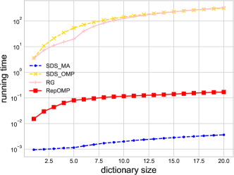
(a) $T=100$, time

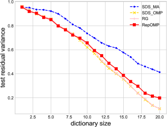
(b) $T=100$, residual

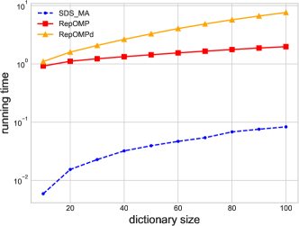
(c) $T=1000$, time

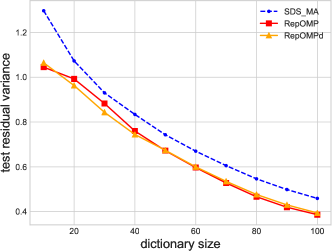
(d) $T=1000$, residual

Figure 3: The experimental results for dimensionality reduced synthetic datasets. In all figures, the horizontal axis indicates the size of the output dictionary. 3(a) and 3(b) are the results for $T=100$. 3(c) and 3(d) are the results for $T=1000$. For each setting, we give the plot of the running time and the test residual variance.

In order to illustrate the advantage of the average sparsity to ordinary dictionary learning (the individual sparsity), we give image restoration examples with real-world images. We use Replacement OMP for both the individual sparsity and the average sparsity. With setting $s_{t}=s$ for all $t\in[T]$, the parameters $k$, $s$, and $s^{\prime}$ are determined with the grid search. We apply Replacement OMP to incomplete images and obtain a dictionary. Then with this dictionary, we repeatedly compute the sparse representation of patches in the input image while shifting a single pixel. OMP is used for obtaining the sparse representation. When calculating the coefficients of the sparse representation of each patch, we use only the observed pixels and restore the whole pixels with these coefficients. We take the median value of all the restored patches for each pixel. In Figure 4, the input image, the image restored with the individual sparsity, and the image restored with the individual sparsity are shown with PSNR ratios. The method with the average sparsity obtains higher PSNR ratios than one with the individual sparsity for all the images.

(a) Input

(b) individual, 34.42dB

(c) average, 34.62dB

(d) Input

(e) individual, 32.18dB

(f) average, 32.25dB

(g) Input

(h) individual, 33.94dB

(i) average, 34.14dB

(j) Input

(k) individual, 33.16dB

(l) average, 33.40dB

Figure 4: The results of the image restoration experiment from images with 80% of pixels missing.

References

- Agarwal et al. [2016] A. Agarwal, A. Anandkumar, P. Jain, and P. Netrapalli. Learning sparsely used overcomplete dictionaries via alternating minimization. SIAM Journal on Optimization, 26(4):2775–2799, 2016.
- Aharon et al. [2006] M. Aharon, M. Elad, and A. Bruckstein. -SVD: An algorithm for designing overcomplete dictionaries for sparse representation. IEEE Transactions on Signal Processing, 54(11):4311–4322, 2006.
- Arora et al. [2014] S. Arora, R. Ge, and A. Moitra. New algorithms for learning incoherent and overcomplete dictionaries. In Proceedings of the Conference on Learning Theory (COLT), pages 779–806, 2014.
- Balkanski et al. [2016] E. Balkanski, B. Mirzasoleiman, A. Krause, and Y. Singer. Learning sparse combinatorial representations via two-stage submodular maximization. In Proceedings of The 33rd International Conference on Machine Learning (ICML), pages 2207–2216, 2016.
- Candes and Tao [2005] E. J. Candes and T. Tao. Decoding by linear programming. IEEE Transactions on Information Theory, 51(12):4203–4215, 2005.
- Cevher and Krause [2011] V. Cevher and A. Krause. Greedy dictionary selection for sparse representation. IEEE Journal of Selected Topics in Signal Processing, 5(5):979–988, 2011.
- Chen et al. [2018] L. Chen, H. Hassani, and A. Karbasi. Online continuous submodular maximization. In Proceedings of the 21st International Conference on Artificial Intelligence and Statistics (AISTATS), volume 84, pages 1896–1905, 2018.
- Cong et al. [2012] Y. Cong, J. Yuan, and J. Luo. Towards scalable summarization of consumer videos via sparse dictionary selection. IEEE Transactions on Multimedia, 14(1):66–75, 2012.
- Cong et al. [2017] Y. Cong, J. Liu, G. Sun, Q. You, Y. Li, and J. Luo. Adaptive greedy dictionary selection for web media summarization. IEEE Transactions on Image Processing, 26(1):185–195, 2017.
- Das and Kempe [2011] A. Das and D. Kempe. Submodular meets spectral: Greedy algorithms for subset selection, sparse approximation and dictionary selection. In Proceedings of the 28th International Conference on Machine Learning (ICML), pages 1057–1064, 2011.
- Dumitrescu and Irofti [2018] B. Dumitrescu and P. Irofti. Dictionary Learning Algorithms and Applications. Springer, 2018.
- Elenberg et al. [2017] E. Elenberg, A. G. Dimakis, M. Feldman, and A. Karbasi. Streaming weak submodularity: Interpreting neural networks on the fly. In Advances in Neural Information Processing Systems (NIPS) 30, pages 4047–4057. 2017.
- Elenberg et al. [2016] E. R. Elenberg, R. Khanna, and A. G. Dimakis. Restricted strong convexity implies weak submodularity. In Proceedings of NIPS Workshop on Learning in High Dimensions with Structure, 2016.
- Engan et al. [1999] K. Engan, S. O. Aase, and J. Hakon Husoy. Method of optimal directions for frame design. In Proceedings of the IEEE International Conference on the Acoustics, Speech, and Signal Processing, volume 05, pages 2443–2446, 1999.
- [15] M. Everingham, A. Zisserman, C. K. I. Williams, and L. Van Gool. The PASCAL Visual Object Classes Challenge 2006 (VOC2006) Results. http://www.pascal-network.org/challenges/VOC/voc2006/results.pdf.
- Foucart and Rauhut [2013] S. Foucart and H. Rauhut. A Mathematical Introduction to Compressive Sensing. Springer, 2013.
- Fujishige [2005] S. Fujishige. Submodular Functions and Optimization. Elsevier, 2nd edition, 2005.
- Golub and Van Loan [2012] G. H. Golub and C. F. Van Loan. Matrix Computations, volume 3. JHU Press, 2012.
- Huang et al. [2009] J. Huang, T. Zhang, and D. Metaxas. Learning with structured sparsity. The Journal of Machine Learning Research, 12:3371–3412, 2009.
- Kale et al. [2017] S. Kale, Z. Karnin, T. Liang, and D. Pál. Adaptive feature selection: Computationally efficient online sparse linear regression under RIP. In Proceedings of the 34th International Conference on Machine Learning (ICML), pages 1–22, 2017.
- Khanna et al. [2017] R. Khanna, E. Elenberg, A. Dimakis, J. Ghosh, and S. Neghaban. On approximation guarantees for greedy low rank optimization. In Proceedings of the 34th International Conference on Machine Learning (ICML), pages 1837–1846, 2017.
- Krause and Cevher [2010] A. Krause and V. Cevher. Submodular dictionary selection for sparse representation. In Proceedings of the 27th International Conference on Machine Learning (ICML), pages 567–574, 2010.
- Liberty and Sviridenko [2017] E. Liberty and M. Sviridenko. Greedy minimization of weakly supermodular set functions. In Approximation, Randomization, and Combinatorial Optimization. Algorithms and Techniques (APPROX/RANDOM 2017), volume 81, pages 19:1–19:11, 2017.
- Mairal et al. [2010] J. Mairal, F. Bach, J. Ponce, and G. Sapiro. Online learning for matrix factorization and sparse coding. Journal of Machine Learning Research, 11:19–60, 2010.
- Natarajan [1995] B. K. Natarajan. Sparse approximate solutions to linear systems. SIAM Journal on Computing, 24(2):227–234, 1995.
- Negahban et al. [2012] S. N. Negahban, P. Ravikumar, M. J. Wainwright, and B. Yu. A unified framework for high-dimensional analysis of -estimators with decomposable regularizers. Statistical Science, 27(4):538–557, 2012.
- Nemhauser et al. [1978] G. L. Nemhauser, L. A. Wolsey, and M. L. Fisher. An analysis of approximations for maximizing submodular set functions - I. Mathematical Programming, 14(1):265–294, 1978.
- Rubinstein et al. [2010] R. Rubinstein, M. Zibulevsky, and M. Elad. Double sparsity: Learning sparse dictionaries for sparse signal approximation. IEEE Transactions on Signal Processing, 58(3):1553–1564, 2010.
- Rusu et al. [2014] C. Rusu, B. Dumitrescu, and S. A. Tsaftaris. Explicit shift-invariant dictionary learning. IEEE Signal Processing Letters, 21(1):6–9, 2014.
- Stan et al. [2017] S. Stan, M. Zadimoghaddam, A. Krause, and A. Karbasi. Probabilistic submodular maximization in sub-linear time. Proceedings of the 34th International Conference on Machine Learning (ICML), pages 3241–3250, 2017.
- Streeter and Golovin [2009] M. Streeter and D. Golovin. An online algorithm for maximizing submodular functions. In Advances in Neural Information Processing Systems (NIPS), pages 1577–1584, 2009.
- Zhou et al. [2009] M. Zhou, H. Chen, L. Ren, G. Sapiro, L. Carin, and J. W. Paisley. Non-parametric bayesian dictionary learning for sparse image representations. In Advances in Neural Information Processing Systems (NIPS) 22, pages 2295–2303. 2009.