A Block Coordinate Ascent Algorithm
for Mean-Variance Optimization

Abstract

Risk management in dynamic decision problems is a primary concern in many fields, including financial investment, autonomous driving, and healthcare. The mean-variance function is one of the most widely used objective functions in risk management due to its simplicity and interpretability. Existing algorithms for mean-variance optimization are based on multi-time-scale stochastic approximation, whose learning rate schedules are often hard to tune, and have only asymptotic convergence proof. In this paper, we develop a model-free policy search framework for mean-variance optimization with finite-sample error bound analysis (to local optima). Our starting point is a reformulation of the original mean-variance function with its Legendre-Fenchel dual, from which we propose a stochastic block coordinate ascent policy search algorithm. Both the asymptotic convergence guarantee of the last iteration’s solution and the convergence rate of the randomly picked solution are provided, and their applicability is demonstrated on several benchmark domains.

1 Introduction

Risk management plays a central role in sequential decision-making problems, common in fields such as portfolio management [Lai et al.,, 2011], autonomous driving [Maurer et al.,, 2016], and healthcare [Parker,, 2009]. A common risk-measure is the variance of the expected sum of rewards/costs and the mean-variance trade-off function [Sobel,, 1982; Mannor and Tsitsiklis,, 2011] is one of the most widely used objective functions in risk-sensitive decision-making. Other risk-sensitive objectives have also been studied, for example, Borkar, [2002] studied exponential utility functions, Tamar et al., [2012] experimented with the Sharpe Ratio measurement, Chow et al., [2018] studied value at risk (VaR) and mean-VaR optimization, Chow and Ghavamzadeh, [2014], Tamar et al., 2015b , and Chow et al., [2018] investigated conditional value at risk (CVaR) and mean-CVaR optimization in a static setting, and Tamar et al., 2015a investigated coherent risk for both linear and nonlinear system dynamics. Compared with other widely used performance measurements, such as the Sharpe Ratio and CVaR, the mean-variance measurement has explicit interpretability and computational advantages [Markowitz et al.,, 2000; Li and Ng,, 2000]. For example, the Sharpe Ratio tends to lead to solutions with less mean return [Tamar et al.,, 2012]. Existing mean-variance reinforcement learning (RL) algorithms [Tamar et al.,, 2012; Prashanth and Ghavamzadeh,, 2013, 2016] often suffer from heavy computational cost, slow convergence, and difficulties in tuning their learning rate schedules. Moreover, all their analyses are asymptotic and no rigorous finite-sample complexity analysis has been reported. Recently, Dalal et al., [2018] provided a general approach to compute finite sample analysis in the case of linear multiple time scales stochastic approximation problems. However, existing multiple time scales algorithms like [Tamar et al.,, 2012] consist of nonlinear term in its update, and cannot be analyzed via the method in Dalal et al., [2018]. All these make it difficult to use them in real-world problems. The goal of this paper is to propose a mean-variance optimization algorithm that is both computationally efficient and has finite-sample analysis guarantees. This paper makes the following contributions: 1) We develop a computationally efficient RL algorithm for mean-variance optimization. By reformulating the mean-variance function with its Legendre-Fenchel dual [Boyd and Vandenberghe,, 2004], we propose a new formulation for mean-variance optimization and use it to derive a computationally efficient algorithm that is based on stochastic cyclic block coordinate descent. 2) We provide the sample complexity analysis of our proposed algorithm. This result is novel because although cyclic block coordinate descent algorithms usually have empirically better performance than randomized block coordinate descent algorithms, yet almost all the reported analysis of these algorithms are asymptotic [Xu and Yin,, 2015].

Here is a roadmap for the rest of the paper. Section 2 offers a brief background on risk-sensitive RL and stochastic variance reduction. In Section 3, the problem is reformulated using the Legendre-Fenchel duality and a novel algorithm is proposed based on stochastic block coordinate descent. Section 4 contains the theoretical analysis of the paper that includes both asymptotic convergence and finite-sample error bound. The experimental results of Section 5 validate the effectiveness of the proposed algorithms.

2 Backgrounds

This section offers a brief overview of risk-sensitive RL, including the objective functions and algorithms. We then introduce block coordinate descent methods. Finally, we introduce the Legendre-Fenchel duality, the key ingredient in formulating our new algorithms.

2.1 Risk-Sensitive Reinforcement Learning

Reinforcement Learning (RL) [Sutton and Barto,, 1998] is a class of learning problems in which an agent interacts with an unfamiliar, dynamic, and stochastic environment, where the agent’s goal is to optimize some measures of its long-term performance. This interaction is conventionally modeled as a Markov decision process (MDP), defined as the tuple $({\mathcal{S},\mathcal{A},P_{0},P_{ss^{\prime}}^{a},r,\gamma})$, where $\mathcal{S}$ and $\mathcal{A}$ are the sets of states and actions, $P_{0}$ is the initial state distribution, $P_{ss^{\prime}}^{a}$ is the transition kernel that specifies the probability of transition from state $s\in\mathcal{S}$ to state $s^{\prime}\in\mathcal{S}$ by taking action $a\in\mathcal{A}$, $r(s,a):\mathcal{S}\times\mathcal{A}\to\mathbb{R}$ is the reward function bounded by $R_{\max}$, and $0\leq\gamma<1$ is a discount factor. A parameterized stochastic policy $\pi_{\theta}(a|s):\mathcal{S}\times\mathcal{A}\to\left[{0,1}\right]$ is a probabilistic mapping from states to actions, where $\theta$ is the tunable parameter and $\pi_{\theta}(a|s)$ is a differentiable function w.r.t. $\theta$.

One commonly used performance measure for policies in episodic MDPs is the return or cumulative sum of rewards from the starting state, i.e., $R=\sum\nolimits_{k=1}^{{\tau}}{r({s_{k}},{a_{k}})}$, where $s_{1}\sim P_{0}$ and $\tau$ is the first passage time to the recurrent state $s^{*}$ [Puterman,, 1994; Tamar et al.,, 2012], and thus, $\tau\coloneqq\min\{k>0\;|\;{s_{k}}={s^{*}}\}$. In risk-neutral MDPs, the algorithms aim at finding a near-optimal policy that maximizes the expected sum of rewards $J(\theta)\coloneqq\mathbb{E}_{\pi_{\theta}}[R]=\mathbb{E}_{\pi_{\theta}}\big{[}\sum_{k=1}^{{\tau}}{r({s_{k}},{a_{k}})}\big{]}$. We also define the square-return $M(\theta)\coloneqq{\mathbb{E}_{{\pi_{\theta}}}}[{R^{2}}]={\mathbb{E}_{{\pi_{\theta}}}}\Big{[}{\big{(}\sum_{k=1}^{\tau}{r({s_{k}},{a_{k}})}\big{)}^{2}}\Big{]}$. In the following, we sometimes drop the subscript $\pi_{\theta}$ to simplify the notation.

In risk-sensitive mean-variance optimization MDPs, the objective is often to maximize $J(\theta)$ with a variance constraint, i.e.,

$$\max_{\theta} J(\theta)=\mathbb{E}_{\pi_{\theta}}[R]$$ (1)

s.t. $$\text{Var}_{\pi_{\theta}}(R)\leq\zeta,$$

where $\text{Var}_{\pi_{\theta}}(R)=M(\theta)-J^{2}(\theta)$ measures the variance of the return random variable $R$, and $\zeta>0$ is a given risk parameter [Tamar et al.,, 2012; Prashanth and Ghavamzadeh,, 2013]. Using the Lagrangian relaxation procedure [Bertsekas,, 1999], we can transform the optimization problem (1) to maximizing the following unconstrained objective function:

$${J_{\lambda}}(\theta)\coloneqq \mathbb{E}_{\pi_{\theta}}[R]-\lambda\big{(}\text{Var}_{\pi_{\theta}}(R)-\zeta)$$ (2)

$$= J(\theta)-\lambda\big{(}M(\theta)-J(\theta)^{2}-\zeta\big{)}.$$ (3)

It is important to note that the mean-variance objective function is NP-hard in general [Mannor and Tsitsiklis,, 2011]. The main reason for the hardness of this optimization problem is that although the variance satisfies a Bellman equation [Sobel,, 1982], unfortunately, it lacks the monotonicity property of dynamic programming (DP), and thus, it is not clear how the related risk measures can be optimized by standard DP algorithms [Sobel,, 1982].

The existing methods to maximize the objective function (3) are mostly based on stochastic approximation that often converge to an equilibrium point of an ordinary differential equation (ODE) [Borkar,, 2008]. For example, Tamar et al., [2012] proposed a policy gradient algorithm, a two-time-scale stochastic approximation, to maximize (3) for a fixed value of $\lambda$ (they optimize over $\lambda$ by selecting its best value in a finite set), while the algorithm in Prashanth and Ghavamzadeh, [2013] to maximize (3) is actor-critic and is a three-time-scale stochastic approximation algorithm (the third time-scale optimizes over $\lambda$). These approaches suffer from certain drawbacks: 1) Most of the analyses of ODE-based methods are asymptotic, with no sample complexity analysis. 2) It is well-known that multi-time-scale approaches are sensitive to the choice of the stepsize schedules, which is a non-trivial burden in real-world problems. 3) The ODE approach does not allow extra penalty functions. Adding penalty functions can often strengthen the robustness of the algorithm, encourages sparsity and incorporates prior knowledge into the problem [Hastie et al.,, 2001].

2.2 Coordinate Descent Optimization

Coordinate descent (CD) and the more general block coordinate descent (BCD) algorithms solve a minimization problem by iteratively updating variables along coordinate directions or coordinate hyperplanes [Wright,, 2015]. At each iteration of BCD, the objective function is (approximately) minimized w.r.t. a coordinate or a block of coordinates by fixing the remaining ones, and thus, an easier lower-dimensional subproblem needs to be solved. A number of comprehensive studies on BCD have already been carried out, such as Luo and Tseng, [1992] and Nesterov, [2012] for convex problems, and Tseng, [2001], Xu and Yin, [2013], and Razaviyayn et al., [2013] for nonconvex cases (also see Wright, 2015 for a review paper). For stochastic problems with a block structure, Dang and Lan, [2015] proposed stochastic block mirror descent (SBMD) by combining BCD with stochastic mirror descent [Beck and Teboulle,, 2003; Nemirovski et al.,, 2009]. Another line of research on this topic is block stochastic gradient coordinate descent (BSG) [Xu and Yin,, 2015]. The key difference between SBMD and BSG is that at each iteration, SBMD randomly picks one block of variables to update, while BSG cyclically updates all block variables.

In this paper, we develop mean-variance optimization algorithms based on both nonconvex stochastic BSG and SBMD. Since it has been shown that the BSG-based methods usually have better empirical performance than their SBMD counterparts, the main algorithm we report, analyze, and evaluate in the paper is BSG-based. We report our SBMD-based algorithm in Appendix C and use it as a baseline in the experiments of Section 5. The finite-sample analysis of our BSG-based algorithm reported in Section 4 is novel because although there exists such analysis for convex stochastic BSG methods [Xu and Yin,, 2015], we are not aware of similar results for their nonconvex version to the best our knowledge.

3 Algorithm Design

In this section, we first discuss the difficulties of using the regular stochastic gradient ascent to maximize the mean-variance objective function. We then propose a new formulation of the mean-variance objective function that is based on its Legendre-Fenchel dual and derive novel algorithms that are based on the recent results in stochastic nonconvex block coordinate descent. We conclude this section with an asymptotic analysis of a version of our proposed algorithm.

3.1 Problem Formulation

In this section, we describe why the vanilla stochastic gradient cannot be used to maximize $J_{\lambda}(\theta)$ defined in Eq. (3). Taking the gradient of $J_{\lambda}(\theta)$ w.r.t. $\theta$, we have

$$\nabla_{\theta}{J_{\lambda}}({\theta_{t}})= {\nabla_{\theta}}J({\theta_{t}})-\lambda{\nabla_{\theta}}{\rm{Var}}(R)$$ (4)

$$= {\nabla_{\theta}}J({\theta_{t}})-\lambda\big{(}\nabla_{\theta}M(\theta)-2J({\theta})\nabla_{\theta}J({\theta})\big{)}.$$ (5)

Computing $\nabla_{\theta}{J_{\lambda}}({\theta_{t}})$ in (5) involves computing three quantities: $\nabla_{\theta}J({\theta}),\nabla_{\theta}M({\theta})$, and $J({\theta})\nabla_{\theta}J({\theta})$. We can obtain unbiased estimates of $\nabla_{\theta}J(\theta)$ and $\nabla_{\theta}M(\theta)$ from a single trajectory generated by the policy $\pi_{\theta}$ using the likelihood ratio method [Williams,, 1992], as $\nabla_{\theta}J({\theta})=\mathbb{E}[{R_{t}}\omega_{t}(\theta)]$ and $\nabla_{\theta}M({\theta})=\mathbb{E}[R_{t}^{2}\omega_{t}(\theta)]$. Note that $R_{t}$ is the cumulative reward of the $t$-th episode, i.e., $R_{t}=\sum\nolimits_{k=1}^{{\tau_{t}}}r_{k}$, which is possibly a nonconvex function, and $\omega_{t}(\theta)=\sum_{k=1}^{{\tau_{t}}}{\nabla_{\theta}\ln{\pi_{\theta}}({a_{k}}|{s_{k}})}$ is the likelihood ratio derivative. In the setting considered in the paper, an episode is the trajectory between two visits to the recurrent state $s^{*}$. For example, the $t$-th episode refers to the trajectory between the ($t$-1)-th and the $t$-th visits to $s^{*}$. We denote by $\tau_{t}$ the length of this episode.

However, it is not possible to compute an unbiased estimate of $J(\theta)\nabla_{\theta}J(\theta)$ without having access to a generative model of the environment that allows us to sample at least two next states $s^{\prime}$ for each state-action pair $(s,a)$. As also noted by Tamar et al., [2012] and Prashanth and Ghavamzadeh, [2013], computing an unbiased estimate of $J(\theta)\nabla_{\theta}J(\theta)$ requires double sampling (sampling from two different trajectories), and thus, cannot be done using a single trajectory. To circumvent the double-sampling problem, these papers proposed multi-time-scale stochastic approximation algorithms, the former a policy gradient algorithm and the latter an actor-critic algorithm that uses simultaneous perturbation methods [Bhatnagar et al.,, 2013]. However, as discussed in Section 2.1, multi-time-scale stochastic approximation approach suffers from several weaknesses such as no available finite-sample analysis and difficult-to-tune stepsize schedules. To overcome these weaknesses, we reformulate the mean-variance objective function and use it to present novel algorithms with in-depth analysis in the rest of the paper.

3.2 Block Coordinate Reformulation

In this section, we present a new formulation for $J_{\lambda}(\theta)$ that is later used to derive our algorithms and do not suffer from the double-sampling problem in estimating $J(\theta)\nabla_{\theta}J(\theta)$. We begin with the following lemma.

Lemma 1.

For the quadratic function $f(z)=z^{2},\;z\in\mathbb{R}$, we define its Legendre-Fenchel dual as $f(z)=z^{2}=\mathop{\max}_{y\in\mathbb{R}}(2zy-{y^{2}})$.

This is a special case of the Lengendre-Fenchel duality [Boyd and Vandenberghe,, 2004] that has been used in several recent RL papers (e.g., Liu et al., 2015; Du et al., 2017; Liu et al., 2018). Let ${F_{\lambda}}(\theta)\coloneqq{\left({J(\theta)+\frac{1}{{2\lambda}}}\right)^{2}}-M(\theta)$, which follows ${F_{\lambda}}(\theta)=\frac{{{J_{\lambda}}(\theta)}}{\lambda}+\frac{1}{{4{\lambda^{2}}}}-\zeta$. Since $\lambda>0$ is a constant, maximizing $J_{\lambda}(\theta)$ is equivalent to maximizing ${F_{\lambda}}(\theta)$. Using Lemma 1 with $z=J(\theta)+\frac{1}{2\lambda}$, we may reformulate ${F_{\lambda}}(\theta)$ as

$${F_{\lambda}}(\theta)=\mathop{\max}_{y}\Big{(}{2y\big{(}J(\theta)+\frac{1}{{2\lambda}}\big{)}-{y^{2}}}\Big{)}-M(\theta).$$ (6)

Using (6), the maximization problem $\mathop{\max}_{\theta}{F_{\lambda}}(\theta)$ is equivalent to

$$\mathop{\max}_{\theta,y} {\hat{f}_{\lambda}}(\theta,y),$$ (7)

where $${{{\hat{f}}_{\lambda}}(\theta,y)\coloneqq 2y\big{(}J(\theta)+\frac{1}{{2\lambda}}\big{)}-{y^{2}}-M(\theta)}.$$

Our optimization problem is now formulated as the standard nonconvex coordinate ascent problem (7). We use three stochastic solvers to solve (7): SBMD method [Dang and Lan,, 2015], BSG method [Xu and Yin,, 2015], and the vanilla stochastic gradient ascent (SGA) method [Nemirovski et al.,, 2009]. We report our BSG-based algorithm in Section 3.3 and leave the details of the SBMD and SGA based algorithms to Appendix C. In the following sections, we denote by $\beta_{t}^{\theta}$ and $\beta_{t}^{y}$ the stepsizes of $\theta$ and $y$, respectively, and by the subscripts $t$ and $k$ the episode and time-step numbers.

3.3 Mean-Variance Policy Gradient

We now present our main algorithm that is based on a block coordinate update to maximize (7). Let ${g}_{t}^{\theta}$ and ${g}_{t}^{y}$ be block gradients and $\tilde{g}_{t}^{\theta}$ and $\tilde{g}_{t}^{y}$ be their sample-based estimations defined as

$$g^{y}_{t}=\mathbb{E}[\tilde{g}^{y}_{t}]=2J(\theta_{t})+\frac{1}{\lambda}-2y_{t}\quad,\quad \tilde{g}^{y}_{t}=2R_{t}+\frac{1}{\lambda}-2y_{t},$$ (8)

$$g^{\theta}_{t}=\mathbb{E}[\tilde{g}^{\theta}_{t}]=2y_{t+1}\nabla_{\theta}{J(\theta_{t})}-\nabla_{\theta}M(\theta_{t})\quad,\quad \tilde{g}^{\theta}_{t}=\left({2y_{t+1}{R_{t}}-{{({R_{t}})}^{2}}}\right){\omega_{t}}({\theta_{t}}).$$ (9)

The block coordinate updates are

$${y_{t+1}}= {y_{t}}+{\beta^{y}_{t}}{\tilde{g}_{t}^{y}},$$ (10)

$${\theta_{t+1}}= {\theta_{t}}+{\beta^{\theta}_{t}}{\tilde{g}_{t}^{\theta}}.$$ (11)

To obtain unbiased estimates of $g^{y}_{t}$ and $g^{\theta}_{t}$, we shall update $y$ (to obtain $y_{t+1}$) prior to computing $g^{\theta}_{t}$ at each iteration. Now it is ready to introduce the Mean-Variance Policy Gradient (MVP) Algorithm 1.

Algorithm 1 Mean-Variance Policy Gradient (MVP)

1:  Input: Stepsizes $\{\beta_{t}^{\theta}\}$ and $\{\beta_{t}^{y}\}$, and number of iterations $N$    Option I: $\{\beta_{t}^{\theta}\}$ and $\{\beta_{t}^{y}\}$ satisfy the Robbins-Monro condition    Option II: $\beta_{t}^{\theta}$ and $\beta_{t}^{y}$ are set to be constants

2:  for episode $t=1,\dotsc,N$ do

3:     Generate the initial state $s_{1}\sim P_{0}$

4:     while $s_{k}\neq s^{*}$ do

5:        Take the action $a_{k}\sim\pi_{\theta_{t}}(a|s_{k})$ and observe the reward $r_{k}$ and next state $s_{k+1}$

6:     end while

7:     Update the parameters

$${R_{t}}= \sum_{k=1}^{\tau_{t}}{{r_{k}}}$$ (12)

$${\omega_{t}}(\theta_{t})= \sum_{k=1}^{{\tau_{t}}}{\nabla_{\theta}\ln{\pi_{\theta_{t}}}({a_{k}}|{s_{k}})}$$ (13)

$${y_{t+1}}= {y_{t}}+{\beta_{t}^{y}}\left(2R_{t}+\frac{1}{\lambda}-2y_{t}\right)$$ (14)

$${\theta_{t+1}}= {\theta_{t}}+{\beta_{t}^{\theta}}\left({2y_{t+1}{R_{t}}-{{({R_{t}})}^{2}}}\right){\omega_{t}}({\theta_{t}})$$ (15)

8:  end for

9:  Output $\bar{x}_{N}$:    Option I: Set $\bar{x}_{N}=x_{N}=[\theta_{N},y_{N}]^{\top}$    Option II: Set $\bar{x}_{N}=x_{z}=[\theta_{z},y_{z}]^{\top}$, where $z$ is uniformly drawn from $\{1,2,\ldots,N\}$

Before presenting our theoretical analysis, we first introduce the assumptions needed for these results.

Assumption 1 (Bounded Gradient and Variance).

There exist constants $G$ and $\sigma$ such that

$$\|\nabla_{y}\hat{f}_{\lambda}(x)\|_{2}\leq G,~{} \|\nabla_{\theta}\hat{f}_{\lambda}(x)\|_{2}\leq G,$$ (16)

$$\mathbb{E}[\|\Delta^{y}_{t}\|_{2}^{2}]\leq{\sigma}^{2},~{} \mathbb{E}[\|\Delta^{\theta}_{t}\|_{2}^{2}]\leq{\sigma}^{2},$$ (17)

for any $t$ and $x$, where $\|\cdot\|_{2}$ denotes the Euclidean norm, ${\Delta}^{y}_{t}\coloneqq\tilde{g}^{y}_{t}-{g}^{y}_{t}$ and ${\Delta}^{\theta}_{t}\coloneqq\tilde{g}^{\theta}_{t}-{g}^{\theta}_{t}$.

Assumption 1 is standard in nonconvex coordinate descent algorithms [Xu and Yin,, 2015; Dang and Lan,, 2015]. We also need the following assumption that is standard in the policy gradient literature.

Assumption 2 (Ergodicity).

The Markov chains induced by all the policies generated by the algorithm are ergodic, i.e., irreducible, aperiodic, and recurrent.

In practice, we can choose either Option I with the result of the final iteration as output or Option II with the result of a randomly selected iteration as output. In what follows in this section, we report an asymptotic convergence analysis of MVP with Option I, and in Section 4, we derive a finite-sample analysis of MVP with Option II.

Theorem 1 (Asymptotic Convergence).

Let $\big{\{}x_{t}=(\theta_{t},y_{t})\big{\}}$ be the sequence of the outputs generated by Algorithm 1 with Option I. If $\{\beta_{t}^{\theta}\}$ and $\{\beta_{t}^{y}\}$ are time-diminishing real positive sequences satisfying the Robbins-Monro condition, i.e., $\sum_{t=1}^{\infty}{\beta_{t}^{\theta}}=\infty$, $\sum_{t=1}^{\infty}{{{(\beta_{t}^{\theta})}^{2}}}<\infty$, $\sum_{t=1}^{\infty}{\beta_{t}^{y}}=\infty$, and $\sum_{t=1}^{\infty}{{{(\beta_{t}^{y})}^{2}}}<\infty$, then Algorithm 1 will converge such that $\;\lim_{t\rightarrow\infty}\mathbb{E}[\|\nabla\hat{f}_{\lambda}(x_{t})\|_{2}]=0$.

The proof of Theorem 1 follows from the analysis in Xu and Yin, [2013]. Due to space constraint, we report it in Appendix A.

Algorithm 1 is a special case of nonconvex block stochastic gradient (BSG) methods. To the best of our knowledge, no finite-sample analysis has been reported for this class of algorithms. Motivated by the recent papers by Nemirovski et al., [2009], Ghadimi and Lan, [2013], Xu and Yin, [2015], and Dang and Lan, [2015], in Section 4, we provide a finite-sample analysis for general nonconvex block stochastic gradient methods and apply it to Algorithm 1 with Option II.

4 Finite-Sample Analysis

In this section, we first present a finite-sample analysis for the general class of nonconvex BSG algorithms [Xu and Yin,, 2013], for which there are no established results, in Section 4.1. We then use these results and prove a finite-sample bound for our MVP algorithm with Option II, that belongs to this class, in Section 4.2. Due to space constraint, we report the detailed proofs in Appendix A.

4.1 Finite-Sample Analysis of Nonconvex BSG Algorithms

In this section, we provide a finite-sample analysis of the general nonconvex block stochastic gradient (BSG) method, where the problem formulation is given by

$$\min_{x\in\mathbb{R}^{n}}~{}f(x)=\mathbb{E}_{\xi}[F(x,\xi)].$$ (18)

$\xi$ is a random vector, and $F(\cdot,\xi):\mathbb{R}^{n}\rightarrow\mathbb{R}$ is continuously differentiable and possibly nonconvex for every $\xi$. The variable $x\in\mathbb{R}^{n}$ can be partitioned into $b$ disjoint blocks as $x=\{x^{1},x^{2},\dotsc,x^{b}\}$, where $x^{i}\in\mathbb{R}^{n_{i}}$ denotes the $i$-th block of variables, and $\sum_{i=1}^{b}n_{i}=n$. For simplicity, we use $x^{<i}$ for $(x_{i},\dots,x_{i-1})$, and $x^{\leq i}$,$x^{>i}$, and $x^{\geq i}$ are defined correspondingly. We also use $\nabla_{x^{i}}$ to denote $\frac{\partial}{\partial x^{i}}$ for the partial gradient with respect to $x^{i}$. $\Xi_{t}$ is the sample set generated at $t$-th iteration, and $\mathbf{\Xi}_{[t]}=(\Xi_{1},\dots,\Xi_{t})$ denotes the history of sample sets from the first through $t$-th iteration. $\{\beta_{t}^{i}:i=1,\cdots,b\}_{t=1}^{\infty}$ are denoted as the stepsizes. Also, let $\beta_{t}^{\max}=\max_{i}\beta_{t}^{i}$, and $\beta_{t}^{\min}=\min_{i}\beta_{t}^{i}$. Similar to Algorithm 1, the BSG algorithm cyclically updates all blocks of variables in each iteration, and the detailed algorithm for BSG method is presented in Appendix B.

Without loss of generality, we assume a fixed update order in the BSG algorithm. Let $\Xi_{t}=\{\xi_{t,1},\dotsc,\xi_{t,m_{t}}\}$ be the samples in the $t$-th iteration with size $m_{t}\geq 1$. Therefore, the stochastic partial gradient is computed as $\tilde{g}_{t}^{i}=\frac{1}{m_{t}}\sum_{l=1}^{m_{t}}\nabla_{x^{i}}F(x_{t+1}^{<i},x_{t}^{\geq i};\xi_{t,l}).$ Similar to Section 3, we define $g_{t}^{i}=\nabla_{x^{i}}f(x_{t+1}^{<i},x_{t}^{\geq i})$, and the approximation error as $\Delta_{t}^{i}=\tilde{g}_{t}^{i}-g_{t}^{i}$. We assume that the objective function $f$ is bounded and Lipschitz smooth, i.e., there exists a positive Lipschitz constant $L>0$ such that $\|\nabla_{x^{i}}f(x)-\nabla_{x^{i}}f(y)\|_{2}\leq L\|x-y\|_{2}$, $\forall i\in\{1,\dots,b\}$ and $\forall x,y\in\mathbb{R}^{n}$. Each block gradient of $f$ is also bounded, i.e., there exist a positive constant $G$ such that $\|\nabla_{x^{i}}f(x)\|_{2}\leq G$, for any $i\in\{1,\dots,b\}$ and any $x\in\mathbb{R}^{n}$. We also need Assumption 1 for all block variables, i.e., $\mathbb{E}[\|\Delta_{t}^{i}\|_{2}]\leq\sigma$, for any $i$ and $t$. Then we have the following lemma.

Lemma 2.

For any $i$ and $t$, there exist a positive constant $A$, such that

$$\|\mathbb{E}[\Delta_{t}^{i}|\mathbf{\Xi}_{[t-1]}]\|_{2}\leq A\beta_{t}^{\max}.$$ (19)

The proof of Lemma 2 is in Appendix B. It should be noted that in practice, it is natural to take the final iteration’s result as the output as in Algorithm 1. However, a standard strategy for analyzing nonconvex optimization methods is to pick up one previous iteration’s result randomly according to a discrete probability distribution over $\{1,2,\dotsc,N\}$ [Nemirovski et al.,, 2009; Ghadimi and Lan,, 2013; Dang and Lan,, 2015]. Similarly, our finite-sample analysis is based on the strategy that randomly pick up $\bar{x}_{N}=x_{z}$ according to

$$\Pr(z=t)=\frac{\beta_{t}^{\min}-\frac{L}{2}(\beta_{t}^{\max})^{2}}{\sum_{t=1}^{N}(\beta_{t}^{\min}-\frac{L}{2}(\beta_{t}^{\max})^{2})},\ t=1,\dotsc,N.$$ (20)

Now we provide the finite-sample analysis result for the general nonconvex BSG algorithm as in [Xu and Yin,, 2015].

Theorem 2.

Let the output of the nonconvex BSG algorithm be $\bar{x}_{N}=x_{z}$ according to Eq. (20). If stepsizes satisfy $2\beta_{t}^{\min}>L(\beta_{t}^{\max})^{2}$ for $t=1,\cdots,N$, then we have

$$\mathbb{E}\left[\|\nabla f(\bar{x}_{N})\|_{2}^{2}\right]\leq\frac{f(x_{1})-f^{*}+\sum_{t=1}^{N}(\beta_{t}^{\max})^{2}C_{t}}{\sum_{t=1}^{N}(\beta_{t}^{\min}-\frac{L}{2}(\beta_{t}^{\max})^{2})},$$ (21)

where $f^{*}=\max_{x}f(x)$. $C_{t}=(1-\frac{L}{2}\beta_{t}^{\max})\sum_{i=1}^{b}L\sqrt{\sum_{j<i}(G^{2}+\sigma^{2})}+b\left(AG+\frac{L}{2}\sigma^{2}\right),$ where $G$ is the gradient bound, $L$ is the Lipschitz constants, $\sigma$ is the variance bound, and $A$ is defined in Eq. (19).

As a special case, we discuss the convergence rate with constant stepsizes $\mathcal{O}(1/\sqrt{N})$ in Corollary 1, which implies that the sample complexity $N=\mathcal{O}(1/\varepsilon^{2})$ in order to find $\varepsilon$-stationary solution of problem (18).

Corollary 1.

If we take constant stepsize such that $\beta_{t}^{i}=\beta^{i}=\mathcal{O}(1/\sqrt{N})$ for any $t$, and let $\beta^{\max}\coloneqq\max_{i}\beta^{i}$, $\beta^{\min}\coloneqq\min_{i}\beta^{i}$, then we have $\mathbb{E}\left[\|\nabla f(\bar{x}_{N})\|_{2}^{2}\right]\leq\mathcal{O}\left(\sqrt{\frac{f(x_{1})-f^{*}+C}{N}}\right),$ where $C_{t}$ in Eq. (21) reduces to a constant $C$ defined as $C=(1-\frac{L}{2}\beta^{\max})\sum_{i=1}^{b}L\sqrt{\sum_{j<i}(G^{2}+\sigma^{2})}+b\left(AG+\frac{L}{2}\sigma^{2}\right).$

4.2 Finite-Sample Analysis of Algorithm 1

We present the major theoretical results of this paper, i.e., the finite-sample analysis of Algorithm 1 with Option II. The proof of Theorem 3 is in Appendix A.

Theorem 3.

Let the output of the Algorithm 1 be $\bar{x}_{N}$ as in Theorem 2. If $\{\beta_{t}^{\theta}\}$, $\{\beta_{t}^{y}\}$ are constants as in Option II in Algorithm 1, and also satisfies $2\beta_{t}^{\min}>L(\beta_{t}^{\max})^{2}$ for $t=1,\cdots,N$, we have

$$\mathbb{E}\left[\|\nabla\hat{f}_{\lambda}(\bar{x}_{N})\|_{2}^{2}\right]\leq\dfrac{\hat{f}_{\lambda}^{*}-\hat{f}_{\lambda}(x_{1})+N(\beta_{t}^{\max})^{2}C}{N(\beta_{t}^{\min}-\frac{L}{2}(\beta_{t}^{\max})^{2})}$$ (22)

where $\hat{f}_{\lambda}^{*}=\max_{x}\hat{f}_{\lambda}(x)$, and

$$C= (1-\dfrac{L}{2}\beta_{t}^{\max})(L^{2}\beta_{t}^{\max}(G^{2}+\sigma^{2})+L(2G^{2}+\sigma^{2}))+AG+L\sigma^{2}+2L(1+L\beta_{t}^{\max})(3\sigma^{2}+2G^{2}).$$ (23)

Proof Sketch.

The proof follows the following major steps.

(I). First, we need to prove the bound of each block coordinate gradient, i.e., $\mathbb{E}[\|g_{t}^{\theta}\|_{2}^{2}]$ and $\mathbb{E}[\|g_{t}^{y}\|_{2}^{2}]$, which is bounded as

$$(\beta_{t}^{\min}-\dfrac{L}{2}(\beta_{t}^{\max})^{2})\mathbb{E}[\|g_{t}^{\theta}\|_{2}^{2}+\|g_{t}^{y}\|_{2}^{2}]$$ (24)

$$\leq \mathbb{E}[\hat{f}_{\lambda}(x_{t+1})]-\mathbb{E}[\hat{f}_{\lambda}(x_{t})]+(\beta_{t}^{\max})^{2}AM_{\rho}+L(\beta_{t}^{\max})^{2}\sigma^{2}+2L\beta_{t}^{\max}(\beta_{t}^{\max}+L(\beta_{t}^{\max})^{2})(3\sigma^{2}+2G^{2}).$$ (25)

Summing up over $t$, we have

$$\sum_{t=1}^{N}(\beta_{t}^{\min}-\dfrac{L}{2}(\beta_{t}^{\max})^{2})\mathbb{E}[\|g_{t}^{\theta}\|_{2}^{2}+\|g_{t}^{y}\|_{2}^{2}]$$ (26)

$$\leq \hat{f}_{\lambda}^{*}-\hat{f}_{\lambda}(x_{1})+\sum_{t=1}^{N}[(\beta_{t}^{\max})^{2}AG+L(\beta_{t}^{\max})^{2}\sigma^{2}+2L\beta_{t}^{\max}(\beta_{t}^{\max}+L(\beta_{t}^{\max})^{2})(3\sigma^{2}+2G^{2})].$$ (27)

(II). Next, we need to bound $\mathbb{E}[\|\nabla\hat{f}_{\lambda}(x_{t})\|_{2}^{2}]$ using $\mathbb{E}[\|g_{t}^{\theta}\|_{2}^{2}+\|g_{t}^{y}\|_{2}^{2}]$, which is proven to be

$$\mathbb{E}[\|\nabla\hat{f}_{\lambda}(x_{t})\|_{2}^{2}]\leq L^{2}(\beta_{t}^{\max})^{2}(G^{2}+\sigma^{2})+L\beta_{t}^{\max}(2G^{2}+\sigma^{2})+\mathbb{E}[\|g_{t}^{\theta}\|_{2}^{2}+\|g_{t}^{y}\|_{2}^{2}].$$ (28)

(III). Finally, combining (I) and (II), and rearranging the terms, Eq. (22) can be obtained as a special case of Theorem 2, which completes the proof. ∎

5 Experimental Study

In this section, we evaluate our MVP algorithm with Option I in three risk-sensitive domains: the portfolio management [Tamar et al.,, 2012], the American-style option [Tamar et al.,, 2014], and the optimal stopping [Chow and Ghavamzadeh,, 2014; Chow et al.,, 2018]. The baseline algorithms are the vanilla policy gradient (PG), the mean-variance policy gradient in Tamar et al., [2012], the stochastic gradient ascent (SGA) applied to our optimization problem (7), and the randomized coordinate ascent policy gradient (RCPG), i.e., the SBMD-based version of our algorithm. Details of SGA and RCPG can be found in Appendix C. For each algorithm, we optimize its Lagrangian parameter $\lambda$ by grid search and report the mean and variance of its return random variable as a Gaussian. Since the algorithms presented in the paper (MVP and RCPG) are policy gradient, we only compare them with Monte-Carlo based policy gradient algorithms and do not use any actor-critic algorithms, such as those in Prashanth and Ghavamzadeh, [2013] and TRPO [Schulman et al.,, 2015], in the experiments.

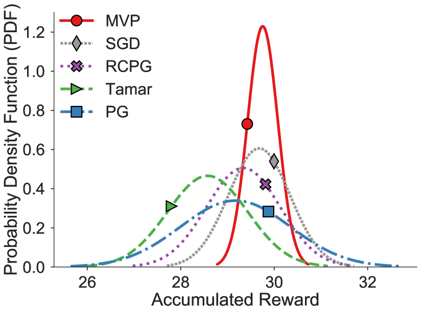
(a) Portfolio management domain

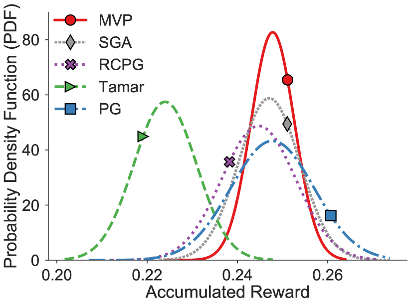
(b) American-style option domain

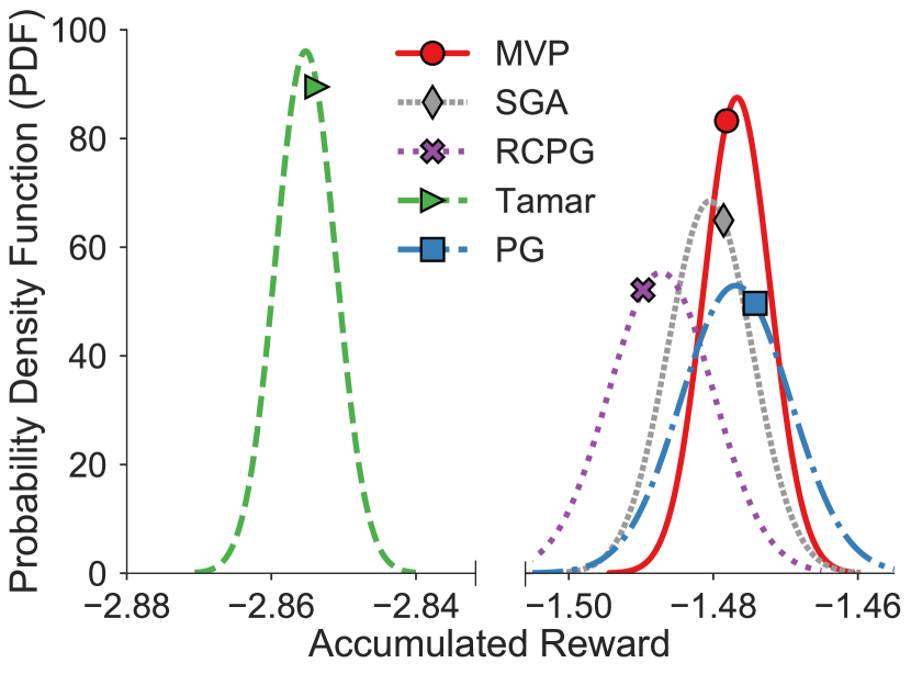
(c) Optimal stopping domain

Figure 1: Empirical results of the distributions of the return (cumulative rewards) random variable. Note that markers only indicate different methods.

5.1 Portfolio Management

The portfolio domain Tamar et al., [2012] is composed of the liquid and non-liquid assets. A liquid asset has a fixed interest rate $r_{l}$ and can be sold at any time-step $k\leq{\tau}$. A non-liquid asset can be sold only after a fixed period of $W$ time-steps with a time-dependent interest rate $r_{\text{nl}}(k)$, which can take either $r_{\text{nl}}^{\text{low}}$ or $r_{\text{nl}}^{\text{high}}$, and the transition follows a switching probability $p_{\text{switch}}$. The non-liquid asset also suffers a default risk (i.e., not being paid) with a probability $p_{\text{risk}}$. All investments are in liquid assets at the initial time-step $k=0$. At the $k$-th step, the state is denoted by $x(k)\in\mathbb{R}^{W+2}$, where $x_{1}\in[0,1]$ is the portion of the investment in liquid assets, $x_{2},\cdots,x_{W+1}\in[0,1]$ is the portion in non-liquid assets with time to maturity of $1,\cdots,W$ time-steps, respectively, and $x_{W+2}(k)=r_{\text{nl}}(k)-\mathbb{E}[r_{\text{nl}}(k)]$. The investor can choose to invest a fixed portion $\eta$ ($0<\eta<1$) of his total available cash in the non-liquid asset or do nothing. More details about this domain can be found in Tamar et al., [2012]. Figure 1(a) shows the results of the algorithms. PG has a large variance and the Tamar’s method has the lowest mean return. The results indicate that MVP yields a higher mean return with less variance compared to the competing algorithms.

5.2 American-style Option

An American-style option Tamar et al., [2014] is a contract that gives the buyer the right to buy or sell the asset at a strike price $W$ at or before the maturity time ${\tau}$. The initial price of the option is $x_{0}$, and the buyer has bought a put option with the strike price $W_{\text{put}}<x_{0}$ and a call option with the strike price $W_{\text{call}}>x_{0}$. At the $k$-th step ($k\leq\tau$), the state is $\{x_{k},k\}$, where $x_{k}$ is the current price of the option. The action $a_{k}$ is either executing the option or holding it. $x_{k+1}$ is $f_{u}x_{k}$ w.p. $p$ and $f_{d}x_{k}$ w.p. $1-p$, where $f_{u}$ and $f_{d}$ are constants. The reward is $0$ unless an option is executed and the reward for executing an option is ${r_{k}}=\max(0,{W_{{\rm{put}}}}-{x_{k}})+\max(0,{x_{k}}-{W_{{\rm{call}}}})$. More details about this domain can be found in Tamar et al., [2014]. Figure 1(b) shows the performance of the algorithms. The results suggest that MVP can yield a higher mean return with less variance compared to the other algorithms.

5.3 Optimal Stopping

The optimal stopping problem [Chow and Ghavamzadeh,, 2014; Chow et al.,, 2018] is a continuous state domain. At the $k$-th time-step ($k\leq\tau$, $\tau$ is the stopping time), the state is $\{x_{k},k\}$, where $x_{k}$ is the cost. The buyer decide either to accept the present cost or wait. If the buyer accepts or when $k=T$, the system reaches a terminal state and the cost $x_{k}$ is received, otherwise, the buyer receives the cost $p_{h}$ and the new state is $\{x_{k+1},k+1\}$, where $x_{k+1}$ is $f_{u}x_{k}$ w.p. $p$ and $f_{d}x_{k}$ w.p. $1-p$ ($f_{u}>1$ and $f_{d}<1$ are constants). More details about this domain can be found in Chow and Ghavamzadeh, [2014]. Figure 1(c) shows the performance of the algorithms. The results indicate that MVP is able to yield much less variance without affecting its mean return. We also summarize the performance of these algorithms in all three risk-sensitive domains as Table 1, where Std is short for Standard Deviation.

	Portfolio Management		American-style Option		Optimal Stopping
	Mean	Std	Mean	Std	Mean	Std
MVP	29.754	0.325	0.2478	0.00482	-1.4767	0.00456
PG	29.170	1.177	0.2477	0.00922	-1.4769	0.00754
Tamar	28.575	0.857	0.2240	0.00694	-2.8553	0.00415
SGA	29.679	0.658	0.2470	0.00679	-1.4805	0.00583
RCPG	29.340	0.789	0.2447	0.00819	-1.4872	0.00721

Table 1: Performance Comparison among Algorithms

6 Conclusion

This paper is motivated to provide a risk-sensitive policy search algorithm with provable sample complexity analysis to maximize the mean-variance objective function. To this end, the objective function is reformulated based on the Legendre-Fenchel duality, and a novel stochastic block coordinate ascent algorithm is proposed with in-depth analysis. There are many interesting future directions on this research topic. Besides stochastic policy gradient, deterministic policy gradient [Silver et al.,, 2014] has shown great potential in large discrete action space. It is interesting to design a risk-sensitive deterministic policy gradient method. Secondly, other reformulations of the mean-variance objective function are also worth exploring, which will lead to new families of algorithms. Thirdly, distributional RL [Bellemare et al.,, 2016] is strongly related to risk-sensitive policy search, and it is interesting to investigate the connections between risk-sensitive policy gradient methods and distributional RL. Last but not least, it is interesting to test the performance of the proposed algorithms together with other risk-sensitive RL algorithms on highly-complex risk-sensitive tasks, such as autonomous driving problems and other challenging tasks.

Appendix A Theoretical Analysis of Algorithm 1

Now we present the theoretical analysis of Algorithm 1, with both asymptotic convergence and finite-sample error bound analysis. For the purpose of clarity, in the following analysis, $x$ is defined as $x:=[y,\theta]^{\top}$, where $x^{1}:=y,\ x^{2}:=\theta$. Similarly, $g_{t}^{i}$ (resp. $\beta^{i}_{t}$) is used to denote $g_{t}^{y}$(resp. $\beta^{y}_{t}$) and $g_{t}^{\theta}$(resp. $\beta^{\theta}_{t}$), where $g_{t}^{1}:=g_{t}^{y},\ g_{t}^{2}:=g_{t}^{\theta}$(resp. $\beta^{1}_{t}:=\beta^{y}_{t},\ \beta^{2}_{t}:=\beta^{\theta}_{t}$). Let $\beta_{t}^{\max}=\max\{\beta_{t}^{1},\beta_{t}^{2}\}$, $\beta_{t}^{\min}=\min\{\beta_{t}^{1},\beta_{t}^{2}\}$, and $\|\cdot\|_{2}$ denotes the Euclidean norm.

A.1 Asymptotic Convergence Proof Algorithm 1

In this section, we provide the asymptotic convergence analysis for Algorithm 1 with Option I, i.e., the stepsizes are chosen to satisfy the Robbins-Monro condition and the output is the last iteration’s result. We first introduce a useful lemma, which follows from Lemma 2.

Lemma 3.

Under Assumption 1, we have

$$\mathbb{E}[\langle\nabla_{y}\hat{f}_{\lambda}(x_{t}),\Delta_{t}^{y}\rangle]= 0$$ (29)

$$\mathbb{E}[\langle\nabla_{\theta}\hat{f}_{\lambda}(x_{t}),\Delta_{t}^{\theta}\rangle]\leq \beta^{\max}_{t}AG,$$ (30)

where $A$ is defined in Eq (19).

Proof.

Let $\Xi_{t}$ denote the history of random samples from the first to the $t$–th episode, then $x_{t}$ is independent of $\Delta_{t}^{i}$ conditioned on $\Xi_{t-1}$ (since $x_{t}$ is deterministic conditioned on $\Xi_{t-1}$). Then we have

$$\mathbb{E}[\langle\nabla_{y}\hat{f}_{\lambda}(x_{t}),\Delta_{t}^{y}\rangle]=\mathbb{E}_{\Xi_{t-1}}[\mathbb{E}[\langle\nabla_{y}\hat{f}_{\lambda}(x_{t}),\Delta_{t}^{y}\rangle|\Xi_{t-1}]]$$ (31)

$$= \mathbb{E}_{\Xi_{t-1}}[\langle\mathbb{E}[\nabla_{y}\hat{f}_{\lambda}(x_{t})|\Xi_{t-1}],\mathbb{E}[\Delta_{t}^{y}|\Xi_{t-1}]\rangle]=0,$$ (32)

$$\mathbb{E}[\langle\nabla_{\theta}\hat{f}_{\lambda}(x_{t}),\Delta_{t}^{\theta}\rangle]=\mathbb{E}_{\Xi_{t-1}}[\mathbb{E}[\langle\nabla_{\theta}\hat{f}_{\lambda}(x_{t}),\Delta_{t}^{\theta}\rangle|\Xi_{t-1}]]$$ (33)

$$= \mathbb{E}_{\Xi_{t-1}}[\langle\mathbb{E}[\nabla_{\theta}\hat{f}_{\lambda}(x_{t})|\Xi_{t-1}],\mathbb{E}[\Delta_{t}^{\theta}|\Xi_{t-1}]\rangle]$$ (34)

$$\leq \mathbb{E}_{\Xi_{t-1}}[\|\mathbb{E}[\nabla_{\theta}\hat{f}_{\lambda}(x_{t})|\Xi_{t-1}]\|_{2}\cdot\|\mathbb{E}[\Delta_{t}^{\theta}|\Xi_{t-1}]\|_{2}]$$ (35)

$$\leq \beta^{\max}_{t}A\mathbb{E}_{\Xi_{t-1}}[\|\mathbb{E}[\nabla_{\theta}\hat{f}_{\lambda}(x_{t})|\Xi_{t-1}]\|_{2}]$$ (36)

$$\leq \beta^{\max}_{t}A\mathbb{E}[\|\nabla_{\theta}\hat{f}_{\lambda}(x_{t})\|_{2}]\leq\beta^{\max}_{t}AG,$$ (37)

where the second equality in both Eq.(32) and Eq.(37) follows from the conditional independence between $x_{t}$ and $\Delta_{t}^{i}$, the second inequality in Eq.(37) follows from Assumption 1, and the last inequality in Eq.(37) follows from the Jensen’s inequality and $G$ is the gradient bound. ∎

Then, we introduce Lemma 4, which is essential for proving Theorem 1.

Lemma 4.

For two non-negative scalar sequences $\{a_{t}\}$ and $\{b_{t}\}$, if $\sum_{t=1}^{\infty}a_{t}=+\infty$ and $\sum_{t=1}^{\infty}a_{t}b_{t}<+\infty$, we then have

$$\mathop{\lim}_{t\to\infty}\inf{b_{t}}=0.$$ (38)

Further, if there exists a constant $K>0$ such that $|b_{t+1}-b_{t}|\leq a_{t}K$, then

$$\lim_{t\rightarrow\infty}b_{t}=0.$$ (39)

The detailed proof can be found in Lemma A.5 of [Mairal,, 2013] and Proposition 1.2.4 of [Bertsekas,, 1999]. Now it is ready to prove Theorem 1.

Proof of Theorem 1.

We define $\Gamma_{t}^{1}:=\hat{f}(x_{t}^{1},x_{t}^{2})-\hat{f}(x_{t+1}^{1},x_{t}^{2}),\Gamma_{t}^{2}:=\hat{f}(x_{t+1}^{1},x_{t}^{2})-\hat{f}(x_{t+1}^{1},x_{t+1}^{2})$ to denote the block update. It turns out that for $i=1,2$, and $\Gamma_{t}^{i}$ can be bounded following the Lipschitz smoothness as

$$\Gamma_{t}^{i}\leq \langle g_{t}^{i},x_{t}^{i}-x_{t+1}^{i}\rangle+\dfrac{L}{2}\|x_{t}^{i}-x_{t+1}^{i}\|_{2}^{2}$$ (40)

$$= -\beta_{t}^{i}\langle g_{t}^{i},\tilde{g}_{t}^{i}\rangle+\dfrac{L}{2}(\beta_{t}^{i})^{2}\|\tilde{g}_{t}^{i}\|_{2}^{2}$$ (41)

$$= -(\beta_{t}^{i}-\dfrac{L}{2}(\beta_{t}^{i})^{2})\|g_{t}^{i}\|_{2}^{2}+\dfrac{L}{2}(\beta_{t}^{i})^{2})\|\Delta_{t}^{i}\|_{2}^{2}-(\beta_{t}^{i}-L(\beta_{t}^{i})^{2})\langle g_{t}^{i},\Delta_{t}^{i}\rangle$$ (42)

$$= -(\beta_{t}^{i}-\dfrac{L}{2}(\beta_{t}^{i})^{2})\|g_{t}^{i}\|_{2}^{2}+\dfrac{L}{2}(\beta_{t}^{i})^{2}\|\Delta_{t}^{i}\|_{2}^{2}$$ (43)

$$-(\beta_{t}^{i}-L(\beta_{t}^{i})^{2})(\langle g_{t}^{i}-\nabla_{x^{i}}\hat{f}_{\lambda}(x_{t}),\Delta_{t}^{i}\rangle+\langle\nabla_{x^{i}}\hat{f}_{\lambda}(x_{t}),\Delta_{t}^{i}\rangle)$$ (44)

where the equalities follow the definition of $\Delta_{t}^{i}$ and the update law of Algorithm 1. We also have the following argument

$$-(\beta_{t}^{i}-L(\beta_{t}^{i})^{2})\langle g_{t}^{i}-\nabla_{x^{i}}\hat{f}_{\lambda}(x_{t}),\Delta_{t}^{i}\rangle$$ (45)

$$\leq |\beta_{t}^{i}-L(\beta_{t}^{i})^{2}|\|\Delta_{t}^{i}\|_{2}\|g_{t}^{i}-\nabla_{x^{i}}\hat{f}_{\lambda}(x_{t})\|_{2}$$ (46)

$$\leq L|\beta_{t}^{i}-L(\beta_{t}^{i})^{2}|\|\Delta_{t}^{i}\|_{2}\|x_{t+1}-x_{t}\|_{2}$$ (47)

$$\leq L|\beta_{t}^{i}-L(\beta_{t}^{i})^{2}|\|\Delta_{t}^{i}\|_{2}\sqrt{\sum_{j=1}^{2}\|\beta_{t}^{j}\tilde{g}_{t}^{j}\|_{2}^{2}}$$ (48)

$$\leq L(\beta_{t}^{i}+L(\beta_{t}^{i})^{2})\beta_{t}^{\max}\left(\|\Delta_{t}^{i}\|_{2}+\sum_{j=1}^{2}(\|g_{t}^{j}\|_{2}^{2}+\|\Delta_{t}^{j}\|_{2}^{2})\right),$$ (49)

where the first inequality follows from Cauchy-Schwarz inequality, the second inequality follows from the Lipschitz smoothness of objective function $\hat{f}_{\lambda}$, the third inequality follows from the update law of Algorithm 1, and the last inequality follows from the triangle inequality. Combining Eq. (44) and Eq. (49), we obtain

$$\Gamma_{t}^{i}\leq -(\beta_{t}^{i}-\dfrac{L}{2}(\beta_{t}^{i})^{2})\|g_{t}^{i}\|_{2}^{2}+\dfrac{L}{2}(\beta_{t}^{i})^{2}\|\Delta_{t}^{i}\|_{2}^{2}$$ (50)

$$-(\beta_{t}^{i}-L(\beta_{t}^{i})^{2})\langle\nabla_{x^{i}}\hat{f}_{\lambda}(x_{t}),\Delta_{t}^{i}\rangle$$ (51)

$$+L(\beta_{t}^{i}+L(\beta_{t}^{i})^{2})\cdot\beta_{t}^{\max}\left(\|\Delta_{t}^{i}\|_{2}^{2}+\sum_{j=1}^{2}(\|g_{t}^{j}\|_{2}^{2}+\|\Delta_{t}^{j}\|_{2}^{2})\right).$$ (52)

Summing Eq. (52) over $i$, then we obtain

$$\hat{f}_{\lambda}(x_{t})-\hat{f}_{\lambda}(x_{t+1})$$ (53)

$$\leq -\sum_{i=1}^{2}(\beta_{t}^{i}-\dfrac{L}{2}(\beta_{t}^{i})^{2})\|g_{t}^{i}\|_{2}^{2}-\sum_{i=1}^{2}(\beta_{t}^{i}-L(\beta_{t}^{i})^{2})\langle\nabla_{x^{i}}\hat{f}_{\lambda}(x_{t}),\Delta_{t}^{i}\rangle$$ (54)

$$+\sum_{i=1}^{2}\left(\dfrac{L}{2}(\beta_{t}^{i})^{2}\|\Delta_{t}^{i}\|_{2}^{2}+L(\beta_{t}^{i}+L(\beta_{t}^{i})^{2})\beta_{t}^{\max}(\|\Delta_{t}^{i}\|_{2}^{2}+\sum_{j=1}^{2}(\|g_{t}^{j}\|_{2}^{2}+\|\Delta_{t}^{j}\|_{2}^{2}))\right).$$ (55)

We also have the following fact,

$$\mathbb{E}[\langle\nabla_{y}\hat{f}_{\lambda}(x_{t}),\Delta_{t}^{y}\rangle]= 0$$ (56)

$$\mathbb{E}[\langle\nabla_{\theta}\hat{f}_{\lambda}(x_{t}),\Delta_{t}^{\theta}\rangle]\leq \beta^{\max}_{t}AG.$$ (57)

We prove this fact in Lemma 3 as a special case of Lemma 2, and the general analysis can be found in Lemma 1 in [Xu and Yin,, 2015]. Taking expectation w.r.t. $t$ on both sides of the inequality Eq. (53), we have

$$\mathbb{E}[\hat{f}_{\lambda}(x_{t})]-\mathbb{E}[\hat{f}_{\lambda}(x_{t+1})]$$ (58)

$$\leq -\sum_{i=1}^{2}(\beta_{t}^{i}-\dfrac{L}{2}(\beta_{t}^{i})^{2})\mathbb{E}[\|g_{t}^{i}\|_{2}^{2}]+(\beta_{t}^{\theta}-L(\beta_{t}^{\theta})^{2})\beta^{\max}_{t}AG$$ (59)

$$+\sum_{i=1}^{2}\left(\dfrac{L}{2}(\beta_{t}^{i})^{2}\mathbb{E}[\|\Delta_{t}^{i}\|_{2}^{2}]+L(\beta_{t}^{i}+L(\beta_{t}^{i})^{2})\beta_{t}^{\max}(\mathbb{E}[\|\Delta_{t}^{i}\|_{2}^{2}]+\sum_{j=1}^{2}(\mathbb{E}[\|g_{t}^{j}\|_{2}^{2}]+\mathbb{E}[\|\Delta_{t}^{j}\|_{2}^{2}]))\right)$$ (60)

$$\leq -\sum_{i=1}^{2}(\beta_{t}^{\min}-\dfrac{L}{2}(\beta_{t}^{\max})^{2})\mathbb{E}[\|g_{t}^{i}\|_{2}^{2}]+(\beta^{\max}_{t})^{2}AG$$ (61)

$$+(L(\beta_{t}^{\max})^{2}\sigma^{2}+2L\beta_{t}^{\max}(\beta_{t}^{\max}+L(\beta_{t}^{\max})^{2})(3\sigma^{2}+2G^{2})),$$ (62)

where the first inequality follows from Eq. (32) and Eq. (37), and the second inequality follows from the boundedness of $\mathbb{E}[\|\Delta_{t}^{i}\|_{2}]$ and $\mathbb{E}[\|g_{t}^{i}\|_{2}]$.

Rearranging Eq. (62), we obtain

$$\sum_{i=1}^{2}(\beta_{t}^{\min}-\dfrac{L}{2}(\beta_{t}^{\max})^{2})\mathbb{E}[\|g_{t}^{i}\|_{2}^{2}]$$ (63)

$$\leq \mathbb{E}[\hat{f}_{\lambda}(x_{t+1})]-\mathbb{E}[\hat{f}_{\lambda}(x_{t})]+(\beta_{t}^{\max})^{2}AM_{\rho}+L(\beta_{t}^{\max})^{2}\sigma^{2}$$ (64)

$$+2L\beta_{t}^{\max}(\beta_{t}^{\max}+L(\beta_{t}^{\max})^{2})(3\sigma^{2}+2G^{2}).$$ (65)

By further assuming $0<\inf_{t}\frac{\{\beta^{\theta}_{t}\}}{\{\beta^{y}_{t}\}}\leq\sup_{t}\frac{\{\beta^{\theta}_{t}\}}{\{\beta^{y}_{t}\}}<\infty$, it can be verified that $\{\beta^{\max}_{t}\}$ and $\{\beta^{\min}_{t}\}$ also satisfy Robbins-Monro condition. Note that $\hat{f}_{\lambda}$ is upper bounded, summing Eq. (65) over $t$ and using the Robbins-Monro condition of $\{\beta^{\theta}_{t}\},\{\beta^{y}_{t}\},\{\beta^{\max}_{t}\},\{\beta^{\min}_{t}\}$, we have

$$\sum_{t=1}^{\infty}\beta_{t}^{\min}\mathbb{E}[\|g_{t}^{i}\|_{2}^{2}]<\infty,~{}\forall i.$$ (66)

Furthermore, let $\xi^{1}_{t}=(x_{t}^{1},x_{t}^{2})$ and $\xi^{2}_{t}=(x_{t+1}^{1},x_{t}^{2})$, then

$$|\mathbb{E}[\|g_{t+1}^{i}\|_{2}^{2}]-\mathbb{E}[\|g_{t}^{i}\|_{2}^{2}]|\leq \mathbb{E}[\|g_{t+1}^{i}+g_{t}^{i}\|_{2}\cdot\|g_{t+1}^{i}-g_{t}^{i}\|_{2}]$$ (67)

$$\leq 2LM_{\rho}\mathbb{E}[\|\xi^{i}_{t+1}-\xi^{i}_{t}\|_{2}]$$ (68)

$$= 2LM_{\rho}\mathbb{E}\left[\sqrt{\sum_{j<i}\|\beta_{t+1}^{j}\tilde{g}_{t+1}^{j}\|_{2}^{2}+\sum_{j\geq i}\|\beta_{t}^{j}\tilde{g}_{t}^{j}\|_{2}^{2}}\right]$$ (69)

$$\leq 2LM_{\rho}\beta_{t}^{\max}\mathbb{E}\left[\sqrt{\sum_{j<i}\|\tilde{g}_{t+1}^{j}\|_{2}^{2}+\sum_{j\geq i}\|\tilde{g}_{t}^{j}\|_{2}^{2}}\right]$$ (70)

$$\leq 2LM_{\rho}\beta_{t}^{\max}\sqrt{\mathbb{E}[\sum_{j<i}\|\tilde{g}_{t+1}^{j}\|_{2}^{2}+\sum_{j\geq i}\|\tilde{g}_{t}^{j}\|_{2}^{2}]}$$ (71)

$$\leq 2LM_{\rho}\beta_{t}^{\max}\sqrt{2(G^{2}+\sigma^{2})},$$ (72)

where the first inequality follows from Jensen’s inequality, the second inequality follows from the definition of gradient bound $G$ and the gradient Lipschitz continuity of $\hat{f}_{\lambda}$, the third inequality follows from the Robbins-Monro condition of $\{\beta_{t}^{y}\}$ and $\{\beta_{t}^{\theta}\}$, and the last two inequalities follow Jensen’s inequality in probability theory.

Combining Eq. (66) and Eq. (72) and according to Lemma 4, we have $\lim_{t\rightarrow\infty}\mathbb{E}[\|g_{t}^{i}\|_{2}]=0$ for $i=1,2$ by Jensen’s inequality. Hence,

$$\mathbb{E}[\|\nabla_{y}\hat{f}_{\lambda}(x_{t})\|_{2}]= \mathbb{E}[\|g_{t}^{y}\|_{2}]$$ (73)

$$\mathbb{E}[\|\nabla_{\theta}\hat{f}_{\lambda}(x_{t})\|_{2}]\leq \mathbb{E}[\|\nabla_{\theta}\hat{f}_{\lambda}(x_{t})-g_{t}^{\theta}\|_{2}]+\mathbb{E}[\|g_{t}^{\theta}\|_{2}]$$ (74)

$$\leq L\cdot\mathbb{E}[\|y_{t+1}-y_{t}\|_{2}]+\mathbb{E}[\|g_{t}^{\theta}\|_{2}]$$ (75)

$$\leq L\beta_{t}^{\max}\mathbb{E}[\|\tilde{g}_{t}^{y}\|_{2}]+\mathbb{E}[\|g_{t}^{\theta}\|_{2}]$$ (76)

$$\leq L\beta_{t}^{\max}\sqrt{G^{2}+\sigma^{2}}+\mathbb{E}[\|g_{t}^{\theta}\|_{2}]$$ (77)

where the first inequality follows from the triangle inequality, the second inequality follows from the Lipschitz continuity of $\hat{f}_{\lambda}$, and the last inequality follows from the same argument for Eq. (72). Also, note that $\lim_{t\rightarrow\infty}\beta_{t}^{\max}=0$, $\lim_{t\rightarrow\infty}L\sqrt{G^{2}+\sigma^{2}}<\infty$, and $\lim_{t\rightarrow\infty}\mathbb{E}[\|g_{t}^{i}\|_{2}]=0$, so that when $t\to\infty$, $L\beta_{t}^{\max}\sqrt{G^{2}+\sigma^{2}}+\mathbb{E}[\|g_{t}^{y}\|_{2}]+\mathbb{E}[\|g_{t}^{\theta}\|_{2}]\to 0$. This completes the proof. ∎

Remark 1.

Different from the stringent two-time-scale setting where one stepsize needs to be “quasi-stationary” compared to the other [Tamar et al.,, 2012], the stepsizes in Algorithm 1 does not have such requirements, which makes it easy to tune in practice.

A.2 Finite-Sample Analysis of Algorithm 1

The above analysis provides asymptotic convergence guarantee of Algorithm 1, however, it is desirable to know the sample complexity of the algorithm in real applications. Motivated by offering RL practitioners confidence in applying the algorithm, we then present the sample complexity analysis with Option II described in Algorithm 1, i.e., the stepsizes are set to be a constant, and the output is randomly selected from $\{x_{1},\cdots,x_{N}\}$ with a discrete uniform distribution. This is a standard strategy for nonconvex stochastic optimization approaches [Dang and Lan,, 2015]. With these algorithmic refinements, we are ready to present the finite-sample analysis as follows. It should be noted that this proof is a special case of the general stochastic nonconvex BSG algorithm analysis provided in Appendix B.2.

Proof of Theorem 3.

The proof of finite-sample analysis starts from the similar idea with asymptotic convergence. The following analysis follows from Eq. (65) in the proof of Theorem 1, but we are using stepsizes $\{\beta_{t}^{\theta}\}$, $\{\beta_{t}^{y}\}$ are constants which satisfy $2\beta_{t}^{\min}>L(\beta_{t}^{\max})^{2}$ for $t=1,\cdots,N$ in this proof.

Summing Eq. (65) over $t$, we have

$$\sum_{t=1}^{N}\sum_{i=1}^{2}(\beta_{t}^{\min}-\dfrac{L}{2}(\beta_{t}^{\max})^{2})\mathbb{E}[\|g_{t}^{i}\|_{2}^{2}]$$ (78)

$$\leq \hat{f}_{\lambda}^{*}-\hat{f}_{\lambda}(x_{1})+\sum_{t=1}^{N}[(\beta_{t}^{\max})^{2}AG+L(\beta_{t}^{\max})^{2}\sigma^{2}+2L\beta_{t}^{\max}(\beta_{t}^{\max}+L(\beta_{t}^{\max})^{2})(3\sigma^{2}+2G^{2})].$$ (79)

Next, we bound $\mathbb{E}[\|\nabla\hat{f}_{\lambda}(x_{t})\|_{2}^{2}]$ using $\mathbb{E}[\|g_{t}^{\theta}\|_{2}^{2}+\|g_{t}^{y}\|_{2}^{2}]$

$$\mathbb{E}[\|\nabla\hat{f}_{\lambda}(x_{t})\|_{2}^{2}]= \mathbb{E}[\|\nabla_{\theta}\hat{f}_{\lambda}(x_{t})\|_{2}^{2}+\|\nabla_{y}\hat{f}_{\lambda}(x_{t})\|_{2}^{2}]$$ (80)

$$\leq \mathbb{E}[\|\nabla_{\theta}\hat{f}_{\lambda}(\theta_{t},y_{t})-\nabla_{\theta}\hat{f}_{\lambda}(\theta_{t},y_{t+1})+\nabla_{\theta}\hat{f}_{\lambda}(\theta_{t},y_{t+1})\|_{2}^{2}+\|g_{t}^{y}\|_{2}^{2}]$$ (81)

$$\leq \mathbb{E}[\|\nabla_{\theta}\hat{f}_{\lambda}(\theta_{t},y_{t})-g_{t}^{\theta}\|_{2}^{2}+\|g_{t}^{\theta}\|_{2}^{2}+2\langle\nabla_{\theta}\hat{f}_{\lambda}(\theta_{t},y_{t})-g_{t}^{\theta},g_{t}^{\theta}\rangle+\|g_{t}^{y}\|_{2}^{2}]$$ (82)

$$\leq \mathbb{E}[\|\nabla_{\theta}\hat{f}_{\lambda}(\theta_{t},y_{t})-g_{t}^{\theta}\|_{2}^{2}+2\langle\nabla_{\theta}\hat{f}_{\lambda}(\theta_{t},y_{t})-g_{t}^{\theta},g_{t}^{\theta}\rangle]+\mathbb{E}[\|g_{t}^{\theta}\|_{2}^{2}+\|g_{t}^{y}\|_{2}^{2}]$$ (83)

$$\leq \mathbb{E}[L^{2}\|y_{t+1}-y_{t}\|_{2}^{2}+2L\|y_{t+1}-y_{t}\|_{2}\cdot\|g_{t}^{\theta}\|_{2}]+\mathbb{E}[\|g_{t}^{\theta}\|_{2}^{2}+\|g_{t}^{y}\|_{2}^{2}]$$ (84)

$$\leq \mathbb{E}[L^{2}(\beta_{t}^{y})^{2}\|\tilde{g}_{t}^{y}\|_{2}^{2}+2L\beta_{t}^{y}\|\tilde{g}_{t}^{y}\|_{2}\cdot\|g_{t}^{\theta}\|_{2}]+\mathbb{E}[\|g_{t}^{\theta}\|_{2}^{2}+\|g_{t}^{y}\|_{2}^{2}]$$ (85)

$$\leq L^{2}(\beta_{t}^{y})^{2}(G^{2}+\sigma^{2})+2L\beta_{t}^{y}\mathbb{E}[\|\tilde{g}_{t}^{y}\|_{2}\cdot\|g_{t}^{\theta}\|_{2}]+\mathbb{E}[\|g_{t}^{\theta}\|_{2}^{2}+\|g_{t}^{y}\|_{2}^{2}]$$ (86)

$$\leq L^{2}(\beta_{t}^{y})^{2}(G^{2}+\sigma^{2})+L\beta_{t}^{y}\mathbb{E}[\|\tilde{g}_{t}^{y}\|_{2}^{2}+\|g_{t}^{\theta}\|_{2}^{2}]+\mathbb{E}[\|g_{t}^{\theta}\|_{2}^{2}+\|g_{t}^{y}\|_{2}^{2}]$$ (87)

$$\leq L^{2}(\beta_{t}^{\max})^{2}(G^{2}+\sigma^{2})+L\beta_{t}^{\max}(2G^{2}+\sigma^{2})+\mathbb{E}[\|g_{t}^{\theta}\|_{2}^{2}+\|g_{t}^{y}\|_{2}^{2}].$$ (88)

Then, combine Eq. (88) with Eq. (78)

$$\sum_{t=1}^{N}(\beta_{t}^{\min}-\dfrac{L}{2}(\beta_{t}^{\max})^{2})\mathbb{E}[\|\nabla\hat{f}_{\lambda}(x_{t})\|_{2}^{2}]$$ (89)

$$\leq \sum_{t=1}^{N}(\beta_{t}^{\min}-\dfrac{L}{2}(\beta_{t}^{\max})^{2})\mathbb{E}[L^{2}(\beta_{t}^{\max})^{2}(G^{2}+\sigma^{2})+L\beta_{t}^{\max}(2G^{2}+\sigma^{2})+\|g_{t}^{\theta}\|_{2}^{2}+\|g_{t}^{y}\|_{2}^{2}]$$ (90)

$$\leq \hat{f}_{\lambda}^{*}-\hat{f}_{\lambda}(x_{1})+\sum_{t=1}^{N}[(\beta_{t}^{\min}-\dfrac{L}{2}(\beta_{t}^{\max})^{2})(L^{2}(\beta_{t}^{\max})^{2}(G^{2}+\sigma^{2})$$ (91)

$$+L\beta_{t}^{\max}(2G^{2}+\sigma^{2}))+(\beta_{t}^{\max})^{2}AG+L(\beta_{t}^{\max})^{2}\sigma^{2}+2L\beta_{t}^{\max}(\beta_{t}^{\max}+L(\beta_{t}^{\max})^{2})(3\sigma^{2}+2G^{2})]$$ (92)

$$\leq \hat{f}_{\lambda}^{*}-\hat{f}_{\lambda}(x_{1})+(\beta_{t}^{\max})^{2}\sum_{t=1}^{N}[(1-\dfrac{L}{2}\beta_{t}^{\max})(L^{2}\beta_{t}^{\max}(G^{2}+\sigma^{2})+L(2M_{\rho}^{2}+\sigma^{2}))+AG+L\sigma^{2}$$ (93)

$$+2L(1+L\beta_{t}^{\max})(3\sigma^{2}+2G^{2})].$$ (94)

Rearrange it, we obtain

$$\mathbb{E}[\|\nabla\hat{f}_{\lambda}(x_{z})\|_{2}^{2}]\leq\dfrac{\hat{f}_{\lambda}^{*}-\hat{f}_{\lambda}(x_{1})+N(\beta_{t}^{\max})^{2}C}{N(\beta_{t}^{\min}-\frac{L}{2}(\beta_{t}^{\max})^{2})},$$ (95)

where

$$C= (1-\dfrac{L}{2}\beta_{t}^{\max})(L^{2}\beta_{t}^{\max}(G^{2}+\sigma^{2})+L(2G^{2}+\sigma^{2}))+AG+L\sigma^{2}+2L(1+L\beta_{t}^{\max})(3\sigma^{2}+2G^{2}).$$ (96)

∎

Remark 2.

In Theorem 3, we have proven the finite-sample analysis of Algorithm 1 with Option II, i.e., constant stepsizes and randomly picked solution. Note that the error bound in Eq. (22) can be simplified as $\mathcal{O}(1/(N\beta_{t}^{\min}))+\mathcal{O}(\beta_{t}^{\max})$. Especially, if $\beta_{t}^{\max}=\beta_{t}^{\min}=\beta_{t}^{\theta}=\beta_{t}^{y}$ are set to be $\Theta(1/\sqrt{N})$, then the convergence rate of Option II in Algorithm 1 is $\mathcal{O}(1/\sqrt{N})$.

Appendix B Proofs in Convergence Analysis of Nonconvex BSG

This section includes proof of Lemma 2 and Algorithm 2. We first provide the pseudo-code for nonconvex BSG method as Algorithm 2.

Algorithm 2 The nonconvex BSG Algorithm

Input: Initial point $x_{1}\in\mathbb{R}^{n}$, stepsizes $\{\beta_{t}^{i}:i=1,\cdots,b\}_{k=1}^{\infty}$, positive integers $\{m_{t}\}_{k=1}^{\infty}$ that indicate the mini-batch sizes, and iteration limit $N$.

1:  for $k=1,2,\dotsc,N$ do

2:     Sample mini batch $\Xi_{t}=\{\xi_{t,1},\xi_{t,2},\dotsc,\xi_{t,m_{t}}\}$.

3:     Specify update order $\pi_{t}^{i}=i$, $i=1,\cdots,b$, or randomly shuffle $\{i=1,\cdots,b\}$ to $\{\pi_{t}^{1},\pi_{t}^{2},\dotsc,\pi_{t}^{b}\}$.

4:     for $i=1,2,\dotsc,b$ do

5:        Compute the stochastic partial gradient for the $\pi_{t}^{i}$th block as

$$\tilde{g}_{t}^{i}=\frac{1}{m_{t}}\sum_{j=1}^{m_{t}}\nabla_{x^{\pi_{t}^{i}}}F(x_{t+1}^{\pi_{t}^{<i}},x_{t}^{\pi_{t}^{\geq i}};\xi_{t,j}).$$ (97)

6:        Update $\pi_{t}^{i}$th block

$$x_{t+1}^{\pi_{t}^{i}}=x_{k}^{\pi_{t}^{i}}-\beta_{t}^{i}\tilde{g}_{t}^{i}.$$ (98)

7:     end for

8:  end for

9:  Return $\bar{x}_{N}=x_{z}$ randomly according to

$$\Pr(z=t)=\frac{\beta_{t}^{\min}-\frac{L}{2}(\beta_{t}^{\max})^{2}}{\sum_{t=1}^{N}(\beta_{t}^{\min}-\frac{L}{2}(\beta_{t}^{\max})^{2})},\ t=1,\dotsc,N.$$ (99)

B.1 Proof of Lemma 2

Proof of Lemma 2.

We prove Lemma 2 for the case of discrete $\xi$, note that the proof still holds for the case of continuous $\xi$ just by using probability density function to replace probability distribution. Without the loss of generality, we assume a fixed update order in Algorithm 2: $\pi_{t}^{i}=i,$ for all $i$ and $t$. Let $\Xi_{t}=\{\xi_{k,1},\xi_{k,2},\dotsc,\xi_{k,m_{t}}\}$ be any mini-batch samples in the $t$-th iteration. Let $\tilde{g}_{\Xi_{t},t}^{i}=\frac{1}{m_{t}}\sum_{j=1}^{m_{t}}\nabla_{x^{i}}F(x_{t+1}^{<i},x_{t}^{\geq i};\xi_{t,j})$ and $g_{\Xi_{t},t}^{i}=\nabla_{x^{i}}f(x_{t+1}^{<i},x_{t}^{\geq i})$, and $x_{\Xi_{t},t+1}^{i}=x_{t}^{i}-\beta_{t}^{i}\tilde{g}_{\Xi_{t},t}^{i}$. Then we have

$$\mathbb{E}[\tilde{g}_{\Xi_{t},t}^{i}|\mathbf{\Xi}_{[t-1]}]= \mathbb{E}_{\Xi_{t}}\left[\frac{1}{m_{t}}\sum_{j=1}^{m_{t}}\nabla_{x^{i}}F(x_{\Xi_{t},t+1}^{<i},x_{t}^{\geq i};\xi_{t,j})\right]$$ (100)

$$= \sum_{\xi_{1},\dotsc,\xi_{m_{t}}}\Pr(\Xi_{t}=\{\xi_{1},\xi_{2},\dotsc,\xi_{m_{t}}\})\frac{1}{m_{t}}\sum_{j=1}^{m_{t}}\nabla_{x^{i}}F(x_{\Xi_{t},t+1}^{<i},x_{t}^{\geq i};\xi_{j}),$$ (101)

and

$$\mathbb{E}[g_{\Xi_{t},t}^{i}|\mathbf{\Xi}_{[t-1]}]= \mathbb{E}_{\Xi_{t}}\left[\nabla_{x^{i}}f(x_{\Xi_{t},t+1}^{<i},x_{t}^{\geq i})\right]$$ (102)

$$= \sum_{\xi^{\prime}_{1},\dotsc,\xi^{\prime}_{m_{t}}}\Pr(\Xi^{\prime}_{t}=\{\xi^{\prime}_{1},\xi^{\prime}_{2},\dotsc,\xi^{\prime}_{m_{t}}\})\nabla_{x^{i}}f(x_{\Xi^{\prime}_{t},t+1}^{<i},x_{t}^{\geq i})$$ (103)

$$= \sum_{\xi^{\prime}_{1},\dotsc,\xi^{\prime}_{m_{t}}}\Pr(\Xi^{\prime}_{t}=\{\xi^{\prime}_{1},\xi^{\prime}_{2},\dotsc,\xi^{\prime}_{m_{t}}\})\sum_{\xi_{l}}\Pr(\xi=\xi_{l})\nabla_{x^{i}}F(x_{\Xi^{\prime}_{t},t+1}^{<i},x_{t}^{\geq i};\xi_{l})$$ (104)

$$= \sum_{\xi^{\prime}_{1},\dotsc,\xi^{\prime}_{m_{t}}}\Pr(\Xi^{\prime}_{t}=\{\xi^{\prime}_{1},\xi^{\prime}_{2},\dotsc,\xi^{\prime}_{m_{t}}\})\sum_{\xi_{1},\dotsc,\xi_{m_{t}}}\Pr(\Xi_{t}=\{\xi_{1},\xi_{2},\dotsc,\xi_{m_{t}}\})$$ (105)

$$\frac{1}{m_{t}}\sum_{j=1}^{m_{t}}\nabla_{x^{i}}F(x_{\Xi^{\prime}_{t},t+1}^{<i},x_{t}^{\geq i};\xi_{j}).$$ (106)

Combine Eq. (101) and Eq. (106), we can obtain the expectation of $\Delta_{t}^{i}$ as

$$\mathbb{E}[\Delta_{t}^{i}|\mathbf{\Xi}_{[t-1]}]= \mathbb{E}[\tilde{g}_{t}^{i}-g_{t}^{i}|\mathbf{\Xi}_{[t-1]}]$$ (107)

$$= \sum_{\xi^{\prime}_{1},\dotsc,\xi^{\prime}_{m_{t}}}\Pr(\Xi^{\prime}_{t}=\{\xi^{\prime}_{1},\xi^{\prime}_{2},\dotsc,\xi^{\prime}_{m_{t}}\})\sum_{\xi_{1},\dotsc,\xi_{m_{t}}}\Pr(\Xi_{t}=\{\xi_{1},\xi_{2},\dotsc,\xi_{m_{t}}\})$$ (108)

$$\frac{1}{m_{t}}\sum_{j=1}^{m_{t}}(\nabla_{x^{i}}F(x_{\Xi_{t},t+1}^{<i},x_{t}^{\geq i};\xi_{j})-\nabla_{x^{i}}F(x_{\Xi^{\prime}_{t},t+1}^{<i},x_{t}^{\geq i};\xi_{j}))$$ (109)

$$= \sum_{\xi^{\prime}_{1},\dotsc,\xi^{\prime}_{m_{t}}}\sum_{\xi_{1},\dotsc,\xi_{m_{t}}}\Pr(\Xi^{\prime}_{t}=\{\xi^{\prime}_{1},\xi^{\prime}_{2},\dotsc,\xi^{\prime}_{m_{t}}\})\Pr(\Xi_{t}=\{\xi_{1},\xi_{2},\dotsc,\xi_{m_{t}}\})$$ (110)

$$\frac{1}{m_{t}}\sum_{j=1}^{m_{t}}(\nabla_{x^{i}}F(x_{\Xi_{t},t+1}^{<i},x_{t}^{\geq i};\xi_{j})-\nabla_{x^{i}}F(x_{\Xi^{\prime}_{t},t+1}^{<i},x_{t}^{\geq i};\xi_{j})).$$ (111)

Note that, since the objection function is Lipschitz smoothness, $F(x;\xi)$ is also Lipschitz smoothness if $\Pr(\xi)>0$, and we use $L$ to denote the maximum Lipschitz constant for all $\Pr(\xi)>0$. Similarly, we can also obtain the gradient of $F(x;\xi)$ is also bounded using same analysis, and we use $G$ to denote the maximum bound for all $\Pr(\xi)>0$. Using these two fact, we have

$$\|\nabla_{x^{i}}F(x_{\Xi_{t},t+1}^{<i},x_{t}^{\geq i};\xi_{j})-\nabla_{x^{i}}F(x_{\Xi^{\prime}_{t},t+1}^{<i},x_{t}^{\geq i};\xi_{j})\|_{2}$$ (112)

$$\leq L\|x_{\Xi_{t},t+1}^{<i}-x_{\Xi^{\prime}_{t},t+1}^{<i}\|_{2}$$ (113)

$$\leq \sum_{l<i}L\|x_{\Xi_{t},t+1}^{l}-x_{\Xi^{\prime}_{t},t+1}^{l}\|_{2}$$ (114)

$$\leq \sum_{l<i}L\beta_{t}^{l}\|\tilde{g}_{\Xi_{t},t}^{l}-\tilde{g}_{\Xi^{\prime}_{t},t}^{l}\|_{2}$$ (115)

$$\leq 2LbG\beta_{t}^{\max}.$$ (116)

Combine Eq. (111) and Eq. (116), we complete the proof as

$$\mathbb{E}[\Delta_{t}^{i}|\mathbf{\Xi}_{[t-1]}]$$ (117)

$$\leq \sum_{\xi^{\prime}_{1},\dotsc,\xi^{\prime}_{m_{t}}}\sum_{\xi_{1},\dotsc,\xi_{m_{t}}}\Pr(\Xi^{\prime}_{t}=\{\xi^{\prime}_{1},\xi^{\prime}_{2},\dotsc,\xi^{\prime}_{m_{t}}\})\Pr(\Xi_{t}=\{\xi_{1},\xi_{2},\dotsc,\xi_{m_{t}}\})2LbG\beta_{t}^{\max}$$ (118)

$$= 2LbG\beta_{t}^{\max},$$ (119)

where the last equation follows from the Law of total probability. This completes the proof. ∎

B.2 Proof of Theorem 2

Let $\beta_{t}^{\max}\coloneqq\max_{i}\beta_{t}^{i}$, $\beta_{t}^{\min}\coloneqq\min_{i}\beta_{t}^{i}$. To establish the convergence rate analysis, we start with Lemma 5.

Lemma 5.

Let $u_{k}$ be a random vector that only depends on $\mathbf{\Xi}_{[t-1]}$. If $u_{t}$ is independent of $\Delta_{t}^{i}$, then

$$\mathbb{E}[\langle u_{t},\Delta_{t}^{i}\rangle]\leq A\beta_{t}^{\max}\mathbb{E}[\|u_{t}\|_{2}],$$ (120)

where $A$ is defined in Eq (19).

Now, it is ready to discuss the main convergence properties of the nonconvex Cyclic SBCD algorithm (Algorithm 2) and provide the rate of convergence for that.

Proof of Lemma 5.

We can obtain the result of Lemma 5 by follows

$$\mathbb{E}[\langle u_{t},\Delta_{t}^{i}\rangle]= \mathbb{E}_{\mathbf{\Xi}_{[t-1]}}\left[\mathbb{E}[\langle u_{t},\Delta_{t}^{i}\rangle|\mathbf{\Xi}_{[t-1]}]\right]$$ (121)

$$\overset{\text{(a)}}{=} \mathbb{E}_{\mathbf{\Xi}_{[t-1]}}\left[\langle\mathbb{E}[u_{t}|\mathbf{\Xi}_{[t-1]}],\mathbb{E}[\Delta_{t}^{i}|\mathbf{\Xi}_{[t-1]}]\rangle\right]$$ (122)

$$\leq \mathbb{E}_{\mathbf{\Xi}_{[t-1]}}\left[\|\mathbb{E}[u_{t}|\mathbf{\Xi}_{[t-1]}]\|_{2}\cdot\|\mathbb{E}[\Delta_{t}^{i}|\mathbf{\Xi}_{[t-1]}]\|_{2}\right]$$ (123)

$$\leq A\beta_{t}^{\max}\mathbb{E}_{\mathbf{\Xi}_{[t-1]}}\left[\|\mathbb{E}[u_{t}|\mathbf{\Xi}_{[t-1]}]\|_{2}\right]$$ (124)

$$\overset{\text{(b)}}{\leq} A\beta_{t}^{\max}\mathbb{E}\left[\|u_{t}\|_{2}\right],$$ (125)

where (a) follows from the conditional independence between $u_{t}$ and $\Delta_{t}^{i}$, and (b) follows from Jensen’s inequality. ∎

Proof of Theorem 2.

From the Lipschitz smoothness, it holds that

$$f(x_{t+1}^{\leq i},x_{t}^{>i})-f(x_{t+1}^{<i},x_{t}^{\geq i})$$ (126)

$$\leq \langle g_{t}^{i},x_{t+1}^{i}-x_{t}^{i}\rangle+\frac{L}{2}\|x_{t+1}^{i}-x_{t}^{i}\|_{2}^{2}$$ (127)

$$= -\beta_{t}^{i}\langle g_{t}^{i},\tilde{g}_{t}^{i}\rangle+\frac{L}{2}(\beta_{t}^{i})^{2}\|\tilde{g}_{t}^{i}\|_{2}^{2}$$ (128)

$$= -(\beta_{t}^{i}-\frac{L}{2}(\beta_{t}^{i})^{2})\|g_{t}^{i}\|_{2}^{2}+\frac{L}{2}(\beta_{t}^{i})^{2}\|\Delta_{t}^{i}\|_{2}^{2}-(\beta_{t}^{i}-L(\beta_{t}^{i})^{2})\langle g_{t}^{i},\Delta_{t}^{i}\rangle$$ (129)

where all the equations follow the definition of $\Delta_{t}^{i}$ and the update law of Algorithm 2.

Summing Eq. (129) over $i$, then we obtain

$$f(x_{t+1})-f(x_{t})\leq-\sum_{i=1}^{b}(\beta_{t}^{i}-\frac{L}{2}(\beta_{t}^{i})^{2})\|g_{t}^{i}\|_{2}^{2}+\sum_{i=1}^{b}\frac{L}{2}(\beta_{t}^{i})^{2}\|\Delta_{t}^{i}\|_{2}^{2}-\sum_{i=1}^{b}(\beta_{t}^{i}-L(\beta_{t}^{i})^{2})\langle g_{t}^{i},\Delta_{t}^{i}\rangle.$$ (130)

Use Lemma 5, we also have the following fact,

$$\mathbb{E}[\langle g_{t}^{i},\Delta_{t}^{i}\rangle]\leq\beta^{\max}_{t}AG.$$ (131)

Taking expectation over Eq. (130), we have

$$\mathbb{E}[f(x_{t+1})]-\mathbb{E}[f(x_{t})]$$ (132)

$$\leq -\sum_{i=1}^{b}(\beta_{t}^{i}-\frac{L}{2}(\beta_{t}^{i})^{2})\mathbb{E}[\|g_{t}^{i}\|_{2}^{2}]+\sum_{i=1}^{b}(\beta_{t}^{i}-L(\beta_{t}^{i})^{2})\beta^{\max}_{t}AG+\sum_{i=1}^{b}\frac{L}{2}(\beta_{t}^{i})^{2}\mathbb{E}[\|\Delta_{t}^{i}\|_{2}^{2}]$$ (133)

$$\leq -(\beta_{t}^{\min}-\frac{L}{2}(\beta_{t}^{\max})^{2})\sum_{i=1}^{b}\mathbb{E}[\|g_{t}^{i}\|_{2}^{2}]+\sum_{i=1}^{b}\left((\beta^{\max}_{t})^{2}AG+\frac{L}{2}(\beta_{t}^{i})^{2}\sigma^{2}\right),$$ (134)

where the first inequality follows from Eq. (131), and the second inequality follows from the boundedness of $\mathbb{E}[\|\Delta_{t}^{i}\|_{2}]$ and $\mathbb{E}[\|g_{t}^{i}\|_{2}]$.

Rearranging Eq. (134), we obtain

$$(\beta_{t}^{\min}-\frac{L}{2}(\beta_{t}^{\max})^{2})\sum_{i=1}^{b}\mathbb{E}[\|g_{t}^{i}\|_{2}^{2}]\leq\mathbb{E}[f(x_{t})]-\mathbb{E}[f(x_{t+1})]+\sum_{i=1}^{b}\left((\beta^{\max}_{t})^{2}AG+\frac{L}{2}(\beta_{t}^{i})^{2}\sigma^{2}\right).$$ (135)

Also, we have

$$\mathbb{E}[\|\nabla_{x^{i}}f(x_{t})\|_{2}]\leq \mathbb{E}[\|\nabla_{x^{i}}f(x_{t})-g_{t}^{i}\|_{2}]+\mathbb{E}[\|g_{t}^{i}\|_{2}]$$ (136)

$$\overset{\text{(a)}}{\leq} L\mathbb{E}[\|x_{t+1}^{<i}-x_{t}^{<i}\|_{2}]+\mathbb{E}[\|g_{t}^{i}\|_{2}]$$ (137)

$$\overset{\text{(b)}}{\leq} L\mathbb{E}\left[\sqrt{\sum_{j<i}\|\beta_{t}^{j}\tilde{g}_{t}^{j}\|_{2}^{2}}\right]+\mathbb{E}[\|g_{t}^{i}\|_{2}]$$ (138)

$$\leq L\beta_{t}^{\max}\mathbb{E}\left[\sqrt{\sum_{j<i}\|\tilde{g}_{t}^{j}\|_{2}^{2}}\right]+\mathbb{E}[\|g_{t}^{i}\|_{2}]$$ (139)

$$\overset{\text{(c)}}{\leq} L\beta_{t}^{\max}\sqrt{\mathbb{E}[\sum_{j<i}\|\tilde{g}_{t}^{j}\|_{2}^{2}]}+\mathbb{E}[\|g_{t}^{i}\|_{2}]$$ (140)

$$\overset{\text{(d)}}{\leq} L\beta_{t}^{\max}\sqrt{\sum_{j<i}(G^{2}+\sigma^{2})}+\mathbb{E}[\|g_{t}^{i}\|_{2}],$$ (141)

where (a) follows from the Lipschitz smoothness of $f$, (b) follows from $x_{t+1}^{j}=x_{t}^{j}-\beta_{t}^{j}\tilde{g}_{t}^{j}$, (c) follows from Jenson’s inequality, and (d) follows from the boundedness of gradient and boundedness of variance.

Summing Eq. (141) over $i$, we can obtain

$$\mathbb{E}[\|\nabla f(x_{t})\|_{2}^{2}]=\sum_{i=1}^{b}\mathbb{E}[\|\nabla_{x^{i}}f(x_{t})\|_{2}]\leq\sum_{i=1}^{b}L\beta_{t}^{\max}\sqrt{\sum_{j<i}(G^{2}+\sigma^{2})}+\sum_{i=1}^{b}\mathbb{E}[\|g_{t}^{i}\|_{2}].$$ (142)

Combine Eq. (142) with Eq. (135), we can obtain

$$(\beta_{t}^{\min}-\frac{L}{2}(\beta_{t}^{\max})^{2})\mathbb{E}[\|\nabla f(x_{t})\|_{2}^{2}]$$ (143)

$$\leq (\beta_{t}^{\min}-\frac{L}{2}(\beta_{t}^{\max})^{2})\sum_{i=1}^{b}L\beta_{t}^{\max}\sqrt{\sum_{j<i}(G^{2}+\sigma^{2})}+(\beta_{t}^{\min}-\frac{L}{2}(\beta_{t}^{\max})^{2})\sum_{i=1}^{b}\mathbb{E}[\|g_{t}^{i}\|_{2}]$$ (144)

$$\leq \mathbb{E}[f(x_{t})]-\mathbb{E}[f(x_{t+1})]+(\beta_{t}^{\min}-\frac{L}{2}(\beta_{t}^{\max})^{2})\sum_{i=1}^{b}L\beta_{t}^{\max}\sqrt{\sum_{j<i}(G^{2}+\sigma^{2})}$$ (145)

$$+\sum_{i=1}^{b}\left((\beta^{\max}_{t})^{2}AG+\frac{L}{2}(\beta_{t}^{i})^{2}\sigma^{2}\right),$$ (146)

where the first inequality follows from substituting Eq. (142) into the left-hand side of Eq. (135), and the second inequality follows from substituting Eq. (142) into the right-hand side of Eq. (135).

Summing Eq. (146) over $t$, we have

$$\sum_{t=1}^{N}(\beta_{t}^{\min}-\frac{L}{2}(\beta_{t}^{\max})^{2})\mathbb{E}[\|\nabla f(x_{t})\|_{2}^{2}]$$ (147)

$$\leq f(x_{1})-f(x^{*})$$ (148)

$$+\sum_{t=1}^{N}\left[(\beta_{t}^{\min}-\frac{L}{2}(\beta_{t}^{\max})^{2})\sum_{i=1}^{b}L\beta_{t}^{\max}\sqrt{\sum_{j<i}(G^{2}+\sigma^{2})}+\sum_{i=1}^{b}\left((\beta^{\max}_{t})^{2}AG+\frac{L}{2}(\beta_{t}^{i})^{2}\sigma^{2}\right)\right]$$ (149)

$$\leq f(x_{1})-f(x^{*})+\sum_{t=1}^{N}(\beta_{t}^{\max})^{2}C_{t}.$$ (150)

where $C_{t}$ is

$$C_{t}= (1-\frac{L}{2}\beta_{t}^{\max})\sum_{i=1}^{b}L\sqrt{\sum_{j<i}(G^{2}+\sigma^{2})}+b\left(AG+\frac{L}{2}\sigma^{2}\right).$$ (151)

Using the probability distribution of $R$ given in Eq. (99), we completes the proof. ∎

Proof of Corollary 1.

Combine these conditions with Eq. (150), we have

$$\sum_{t=1}^{N}(\beta^{\min}-\frac{L}{2}(\beta^{\max})^{2})\mathbb{E}[\|\nabla f(x_{t})\|_{2}^{2}]\leq f(x_{1})-f(x^{*})+N(\beta^{\max})^{2}C,$$ (152)

where $C$ is

$$C= (1-\frac{L}{2}\beta^{\max})\sum_{i=1}^{b}L\sqrt{\sum_{j<i}(G_{j}^{2}+\sigma^{2})}+b\left(AG+\frac{L}{2}\sigma^{2}\right).$$ (153)

Using the probability distribution of $z$ given in Eq. (99), we can obtain

$$\mathbb{E}\left[\|\nabla f(x_{z})\|_{2}^{2}\right]\leq\frac{f(x_{1})-f^{*}+N(\beta^{\max})^{2}C}{N(\beta^{\min}-\frac{L}{2}(\beta^{\max})^{2})}.$$ (154)

Thus, we can reach the rate of convergence of $\mathcal{O}(1/\sqrt{N})$ by setting $\beta^{\min}=\beta^{\max}=\mathcal{O}(1/\sqrt{N})$. ∎

Appendix C RCPG and SGA Algorithm

C.1 Randomized Stochastic Block Coordinate Descent Algorithm

We propose the randomized stochastic block coordinate descent algorithm as Algorithm 3. Note that we also use the same notation about gradient from Eq. (8) and Eq. (9) with very a tiny difference in practical, where $y_{t+1}=y_{t}$ in Eq. (9).

Algorithm 3 Risk-Sensitive Randomized Coordinate Descent Policy Gradient (RCPG)

1:  Input: Stepsizes $\{\beta_{t}^{\theta}\}$ and $\{\beta_{t}^{y}\}$, let $\beta_{t}^{\max}=\max\{\beta_{t}^{\theta},\beta_{t}^{y}\}$.Option I: $\{\beta_{t}^{\theta}\}$ and $\{\beta_{t}^{y}\}$ satisfy the Robbins-Monro condition.Option II: $\beta_{t}^{\theta}$ and $\beta_{t}^{y}$ are set to be constants.

2:  for episode $t=1,\dotsc,N$ do

3:     for time step $k=1,\dotsc,{\tau_{t}}$ do

4:        Compute $a_{k}\sim\pi_{\theta}(a|s_{k})$, observe $r_{k},s_{k+1}$.

5:     end for

6:     Compute

$${R_{t}} =\sum_{k=1}^{\tau_{t}}{{r_{k}}}$$ (155)

$${\omega_{t}}(\theta_{t}) =\sum_{k=1}^{{\tau_{t}}}{\nabla_{\theta}\ln{\pi_{\theta_{t}}}({a_{k}}|{s_{k}})}.$$ (156)

7:     Randomly select $i_{t}\in\{1,2\}$ with distribution $[0.5,0.5]$. If $i_{t}=1$,

$${y_{t+1}} ={y_{t}}+{\beta_{t}}\left(2R_{t}+\frac{1}{\lambda}-2y_{t}\right),$$ (157)

$${\theta_{t+1}} ={\theta_{t}}.$$ (158)

else

$${y_{t+1}} ={y_{t}},$$ (159)

$${\theta_{t+1}} ={\theta_{t}}+{\beta_{t}}\left({2y_{t}{R_{t}}-{{({R_{t}})}^{2}}}\right){\omega_{t}}({\theta_{t}}).$$ (160)

8:  end for

9:  Output $\bar{x}_{N}$: Option I: Set $\bar{x}_{N}=x_{N}$. Option II: Set $\bar{x}_{N}=x_{z}$, where $z$ is uniformly drawn from $\{1,2,\dotsc,N\}$.

Note that, the main difference between Cyclic SBCD and Randomized SBCD is that: at each iteration, Cyclic SBCD cyclically updates all blocks of variables, and the later updated blocks depending on the early updated blocks; while Randomized SBCD randomly chooses one block of variables to update.

C.2 Risk-Sensitive Stochastic Gradient Ascent Policy Gradient

We also proposed risk-sensitive stochastic gradient Ascent policy gradient as Algorithm 4.

Algorithm 4 Risk-Sensitive Stochastic Gradient Ascent Policy Gradient (SGA)

1:  Input: Stepsizes $\{\beta_{t}^{\theta}\}$ and $\{\beta_{t}^{y}\}$, let $\beta_{t}^{\max}=\max\{\beta_{t}^{\theta},\beta_{t}^{y}\}$.Option I: $\{\beta_{t}^{\theta}\}$ and $\{\beta_{t}^{y}\}$ satisfy the Robbins-Monro condition.Option II: $\beta_{t}^{\theta}$ and $\beta_{t}^{y}$ are set to be constants.

2:  for episode $t=1,\dotsc,N$ do

3:     for time step $k=1,\dotsc,{\tau_{t}}$ do

4:        Compute $a_{k}\sim\pi_{\theta}(a|s_{k})$, observe $r_{k},s_{k+1}$.

5:     end for

6:     Compute

$${R_{t}} =\sum_{k=1}^{\tau_{t}}{{r_{k}}}$$ (161)

$${\omega_{t}}(\theta_{t}) =\sum_{k=1}^{{\tau_{t}}}{\nabla_{\theta}\ln{\pi_{\theta_{t}}}({a_{k}}|{s_{k}})}.$$ (162)

7:     Update parameters,

$${y_{t+1}} ={y_{t}}+{\beta_{t}}\left(2R_{t}+\frac{1}{\lambda}-2y_{t}\right),$$ (163)

$${\theta_{t+1}} ={\theta_{t}}+{\beta_{t}}\left({2y_{t}{R_{t}}-{{({R_{t}})}^{2}}}\right){\omega_{t}}({\theta_{t}}).$$ (164)

8:  end for

9:  Output $\bar{x}_{N}$: Option I: Set $\bar{x}_{N}=x_{N}$. Option II: Set $\bar{x}_{N}=x_{z}$, where $z$ is uniformly drawn from $\{1,2,\dotsc,N\}$.

Appendix D Details of the Experiments

The parameter settings for portfolio management domain are as follows: $\tau=50$, $r_{l}=1.001$, $r_{\text{nl}}^{\text{high}}=2$, $r_{\text{nl}}^{\text{low}}=1.1$, $p_{\text{risk}}=0.05$, $p_{\text{switch}}=0.1$, $W=4$, $\eta=0.2$, startup cash $\$100,000$.

The parameter settings of American-style Option domain are as follows: $K_{\text{put}}=1$, $K_{\text{call}}=1.5$, $x_{0}=1.25$, $f_{u}=9/8$, $f_{d}=8/9$, $p=0.45$, $\tau=20$.

The parameter settings of optimal stopping domain are as follows: $x_{0}=1.25$, $f_{u}=2$, $f_{d}=0.5$, $p=0.65$, $\tau=20$.

References

- Beck and Teboulle, [2003] Beck, A. and Teboulle, M. (2003). Mirror descent and nonlinear projected subgradient methods for convex optimization. Operations Research Letters, 31:167–175.
- Bellemare et al., [2016] Bellemare, M. G., Dabney, W., and Munos, R. (2016). A distributional perspective on reinforcement learning. In International Conference on Machine Learning.
- Bertsekas, [1999] Bertsekas, D. P. (1999). Nonlinear programming. Athena scientific Belmont.
- Bhatnagar et al., [2013] Bhatnagar, S., Prasad, H., and Prashanth, L. (2013). Stochastic Recursive Algorithms for Optimization, volume 434. Springer.
- Borkar, [2002] Borkar, V. (2002). Q-learning for risk-sensitive control. Mathematics of operations research, 27(2):294–311.
- Borkar, [2008] Borkar, V. (2008). Stochastic Approximation: A Dynamical Systems Viewpoint. Cambridge University Press.
- Boyd and Vandenberghe, [2004] Boyd, S. and Vandenberghe, L. (2004). Convex Optimization. Cambridge University Press.
- Chow and Ghavamzadeh, [2014] Chow, Y. and Ghavamzadeh, M. (2014). Algorithms for CVaR optimization in MDPs. In Advances in Neural Information Processing Systems, pages 3509–3517.
- Chow et al., [2018] Chow, Y., Ghavamzadeh, M., Janson, L., and Pavone, M. (2018). Risk-constrained reinforcement learning with percentile risk criteria. Journal of Machine Learning Research.
- Dalal et al., [2018] Dalal, G., Thoppe, G., Szörényi, B., and Mannor, S. (2018). Finite sample analysis of two-timescale stochastic approximation with applications to reinforcement learning. In Bubeck, S., Perchet, V., and Rigollet, P., editors, Proceedings of the 31st Conference On Learning Theory, pages 1199–1233. PMLR.
- Dang and Lan, [2015] Dang, C. D. and Lan, G. (2015). Stochastic block mirror descent methods for nonsmooth and stochastic optimization. SIAM Journal on Optimization, 25(2):856–881.
- Du et al., [2017] Du, S. S., Chen, J., Li, L., Xiao, L., and Zhou, D. (2017). Stochastic variance reduction methods for policy evaluation. arXiv preprint arXiv:1702.07944.
- Ghadimi and Lan, [2013] Ghadimi, S. and Lan, G. (2013). Stochastic first-and zeroth-order methods for nonconvex stochastic programming. SIAM Journal on Optimization, 23(4):2341–2368.
- Hastie et al., [2001] Hastie, T., Tibshirani, R., and Friedman, J. (2001). The Elements of Statistical Learning. Springer.
- Lai et al., [2011] Lai, T., Xing, H., and Chen, Z. (2011). Mean-variance portfolio optimization when means and covariances are unknown. The Annals of Applied Statistics, pages 798–823.
- Li and Ng, [2000] Li, D. and Ng, W. (2000). Optimal dynamic portfolio selection: Multiperiod mean-variance formulation. Mathematical Finance, 10(3):387–406.
- Liu et al., [2018] Liu, B., Gemp, I., Ghavamzadeh, M., Liu, J., Mahadevan, S., and Petrik, M. (2018). Proximal gradient temporal difference learning: Stable reinforcement learning with polynomial sample complexity. Journal of Artificial Intelligence Research.
- Liu et al., [2015] Liu, B., Liu, J., Ghavamzadeh, M., Mahadevan, S., and Petrik, M. (2015). Finite-sample analysis of proximal gradient td algorithms. In Conference on Uncertainty in Artificial Intelligence.
- Luo and Tseng, [1992] Luo, Z. and Tseng, P. (1992). On the convergence of the coordinate descent method for convex differentiable minimization. Journal of Optimization Theory and Applications, 72(1):7–35.
- Mairal, [2013] Mairal, J. (2013). Stochastic majorization-minimization algorithms for large-scale optimization. In Advances in Neural Information Processing Systems, pages 2283–2291.
- Mannor and Tsitsiklis, [2011] Mannor, S. and Tsitsiklis, J. (2011). Mean-variance optimization in markov decision processes. In Proceedings of the 28th International Conference on Machine Learning (ICML-11).
- Markowitz et al., [2000] Markowitz, H. M., Todd, G. P., and Sharpe, W. F. (2000). Mean-variance analysis in portfolio choice and capital markets, volume 66. John Wiley & Sons.
- Maurer et al., [2016] Maurer, M., Gerdes, C., Lenz, B., and Winner, H. (2016). Autonomous driving: technical, legal and social aspects. Springer.
- Nemirovski et al., [2009] Nemirovski, A., Juditsky, A., Lan, G., and Shapiro, A. (2009). Robust stochastic approximation approach to stochastic programming. SIAM Journal on optimization, 19(4):1574–1609.
- Nesterov, [2012] Nesterov, Y. (2012). Efficiency of coordinate descent methods on huge-scale optimization problems. SIAM Journal on Optimization, 22(2):341–362.
- Parker, [2009] Parker, D. (2009). Managing risk in healthcare: understanding your safety culture using the manchester patient safety framework. Journal of nursing management, 17(2):218–222.
- Prashanth and Ghavamzadeh, [2013] Prashanth, L. A. and Ghavamzadeh, M. (2013). Actor-critic algorithms for risk-sensitive mdps. In Advances in Neural Information Processing Systems, pages 252–260.
- Prashanth and Ghavamzadeh, [2016] Prashanth, L. A. and Ghavamzadeh, M. (2016). Variance-constrained actor-critic algorithms for discounted and average reward mdps. Machine Learning Journal, 105(3):367–417.
- Puterman, [1994] Puterman, M. L. (1994). Markov Decision Processes. Wiley Interscience, New York, USA.
- Razaviyayn et al., [2013] Razaviyayn, M., Hong, M., and Luo, Z. (2013). A unified convergence analysis of block successive minimization methods for nonsmooth optimization. SIAM Journal on Optimization, 23(2):1126–1153.
- Schulman et al., [2015] Schulman, J., Levine, S., Abbeel, P., Jordan, M., and Moritz, P. (2015). Trust region policy optimization. In International Conference on Machine Learning, pages 1889–1897.
- Silver et al., [2014] Silver, D., Lever, G., Heess, N., Degris, T., Wierstra, D., and Riedmiller, M. (2014). Deterministic policy gradient algorithms. In ICML, pages 387–395.
- Sobel, [1982] Sobel, M. J. (1982). The variance of discounted markov decision processes. Journal of Applied Probability, 19(04):794–802.
- Sutton and Barto, [1998] Sutton, R. and Barto, A. G. (1998). Reinforcement Learning: An Introduction. MIT Press.
- Tamar et al., [2012] Tamar, A., Castro, D., and Mannor, S. (2012). Policy gradients with variance related risk criteria. In ICML, pages 935–942.
- [36] Tamar, A., Chow, Y., Ghavamzadeh, M., and Mannor, S. (2015a). Policy gradient for coherent risk measures. In NIPS, pages 1468–1476.
- [37] Tamar, A., Glassner, Y., and Mannor, S. (2015b). Optimizing the cvar via sampling. In AAAI Conference on Artificial Intelligence.
- Tamar et al., [2014] Tamar, A., Mannor, S., and Xu, H. (2014). Scaling up robust mdps using function approximation. In International Conference on Machine Learning, pages 181–189.
- Tseng, [2001] Tseng, P. (2001). Convergence of a block coordinate descent method for nondifferentiable minimization. Journal of optimization theory and applications, 109(3):475–494.
- Williams, [1992] Williams, R. (1992). Simple statistical gradient-following algorithms for connectionist reinforcement learning. Machine learning, 8(3-4):229–256.
- Wright, [2015] Wright, S. (2015). Coordinate descent algorithms. Mathematical Programming, 151(1):3–34.
- Xu and Yin, [2013] Xu, Y. and Yin, W. (2013). A block coordinate descent method for regularized multiconvex optimization with applications to nonnegative tensor factorization and completion. SIAM Journal on imaging sciences, 6(3):1758–1789.
- Xu and Yin, [2015] Xu, Y. and Yin, W. (2015). Block stochastic gradient iteration for convex and nonconvex optimization. SIAM Journal on Optimization, 25(3):1686–1716.