Cell-aware Stacked LSTMs for Modeling Sentences

Abstract

We propose a method of stacking multiple long short-term memory (LSTM) layers for modeling sentences. In contrast to the conventional stacked LSTMs where only hidden states are fed as input to the next layer, the suggested architecture accepts both hidden and memory cell states of the preceding layer and fuses information from the left and the lower context using the soft gating mechanism of LSTMs. Thus the architecture modulates the amount of information to be delivered not only in horizontal recurrence but also in vertical connections, from which useful features extracted from lower layers are effectively conveyed to upper layers. We dub this architecture Cell-aware Stacked LSTM (CAS-LSTM) and show from experiments that our models bring significant performance gain over the standard LSTMs on benchmark datasets for natural language inference, paraphrase detection, sentiment classification, and machine translation. We also conduct extensive qualitative analysis to understand the internal behavior of the suggested approach.

1 Introduction

In the field of natural language processing (NLP), one of the most prevalent neural approaches to obtaining sentence representations is to use recurrent neural networks (RNNs), where words in a sentence are processed in a sequential and recurrent manner. Along with their intuitive design, RNNs have shown outstanding performance across various NLP tasks e.g. language modeling (Mikolov et al., 2010; Graves, 2013), machine translation (Cho et al., 2014; Sutskever et al., 2014; Bahdanau et al., 2015), text classification (Zhou et al., 2015; Tang et al., 2015), and parsing (Kiperwasser and Goldberg, 2016; Dyer et al., 2016).

Among several variants of the original RNN (Elman, 1990), gated recurrent architectures such as long short-term memory (LSTM) (Hochreiter and Schmidhuber, 1997) and gated recurrent unit (GRU) (Cho et al., 2014) have been accepted as de-facto standard choices for RNNs due to their capability of addressing the vanishing and exploding gradient problem and considering long-term dependencies. Gated RNNs achieve these properties by introducing additional gating units that learn to control the amount of information to be transferred or forgotten (Goodfellow et al., 2016), and are proven to work well without relying on complex optimization algorithms or careful initialization (Sutskever, 2013).

Meanwhile, the common practice for further enhancing the expressiveness of RNNs is to stack multiple RNN layers, each of which has distinct parameter sets (stacked RNN) (Schmidhuber, 1992; El Hihi and Bengio, 1996). In stacked RNNs, the hidden states of a layer are fed as input to the subsequent layer, and they are shown to work well due to increased depth (Pascanu et al., 2014) or their ability to capture hierarchical time series (Hermans and Schrauwen, 2013) which are inherent to the nature of the problem being modeled.

However this setting of stacking RNNs might hinder the possibility of more sophisticated structures since the information from lower layers is simply treated as input to the next layer, rather than as another class of state that participates in core RNN computations. Especially for gated RNNs such as LSTMs and GRUs, this means that the vertical layer-to-layer connections cannot fully benefit from the carefully constructed gating mechanism used in temporal transitions.

In this paper, we study a method of constructing multi-layer LSTMs where memory cell states from the previous layer are used in controlling the vertical information flow. This system utilizes states from the left and the lower context equally in computation of the new state, thus the information from lower layers is elaborately filtered and reflected through a soft gating mechanism. Our method is easy-to-implement, effective, and can replace conventional stacked LSTMs without much modification of the overall architecture.

We call this architecture Cell-aware Stacked LSTM, or CAS-LSTM, and evaluate our method on multiple benchmark tasks: natural language inference, paraphrase identification, sentiment classification, and machine translation. From experiments we show that the CAS-LSTMs consistently outperform typical stacked LSTMs, opening the possibility of performance improvement of architectures based on stacked LSTMs.

Our contribution is summarized as follows. Firstly, we bring the idea of utilizing states coming from multiple directions to construction of stacked LSTM and apply the idea to the research of sentence representation learning. There is some prior work addressing the idea of incorporating more than one type of state (Graves et al., 2007; Kalchbrenner et al., 2016; Zhang et al., 2016), however to the best of our knowledge there is little work on applying the idea to modeling sentences for better understanding of natural language text.

Secondly, we conduct extensive evaluation of the proposed method and empirically prove its effectiveness. The CAS-LSTM architecture provides consistent performance gains over the stacked LSTM in all benchmark tasks: natural language inference, paraphrase identification, sentiment classification, and machine translation. Especially in SNLI, SST-2, and Quora Question Pairs datasets, our models outperform or at least are on par with the state-of-the-art models. We also conduct thorough qualitative analysis to understand the dynamics of the suggested approach.

This paper is organized in the following way. We study prior work related to our objective in §2, and §3 gives a detailed description about the proposed method. Experimental results are given in §4, and §5 concludes this paper.

2 Related Work

In this section, we summarize prior work related to the proposed method. We group the previous work that motivated our work into three classes: i) enhancing interaction between vertical layers, ii) RNN architectures that accepts latticed data, and iii) tree-structured RNNs.

Stacked RNNs.

There is some prior work on methods of stacking RNNs beyond the plain stacked RNNs (Schmidhuber, 1992; El Hihi and Bengio, 1996). Residual LSTMs (Kim et al., 2017; Tran et al., 2017) add residual connections between the hidden states computed at each LSTM layer, and shortcut-stacked LSTMs (Nie and Bansal, 2017) concatenate hidden states from all previous layers to make the backpropagation path short. In our method, the lower context is aggregated via a gating mechanism, and we believe it modulates the amount of information to be transmitted in a more efficient and effective way than vector addition or concatenation. Also, compared to concatenation, our method does not significantly increase the number of parameters.

Highway LSTMs (Zhang et al., 2016) and depth-gated LSTMs (Yao et al., 2015) are similar to our proposed models in that they use cell states from the previous layer, and they are successfully applied to the field of automatic speech recognition and language modeling. However in contrast to CAS-LSTM, where the additional forget gate aggregates the previous layer states and thus contexts from the left and below participate in computation equitably, in Highway LSTMs and depth-gated LSTMs the states from the previous time step are not considered in computing vertical gates. The comparison of our method and this architecture is presented in §4.6.

Multidimensional RNNs.

There is another line of research that aims to extend RNNs to operate with multidimensional inputs. Grid LSTMs (Kalchbrenner et al., 2016) are a general $n$-dimensional LSTM architecture that accepts $n$ sets of hidden and cell states as input and yields $n$ sets of states as output, in contrast to our architecture, which emits a single set of states. In their work, the authors utilize 2D and 3D Grid LSTMs in character-level language modeling and machine translation respectively and achieve performance improvement. Multidimensional RNNs (Graves et al., 2007; Graves and Schmidhuber, 2009) have similar formulation to ours, except that they reflect cell states via simple summation and weights for all columns (vertical layers in our case) are tied. However they are only employed to model multidimensional data such as images of handwritten text with RNNs, rather than stacking RNN layers for modeling sequential data. From this view, CAS-LSTM could be interpreted as an extension of two-dimensional LSTM architecture that accepts a 2D input $\{\mathbf{h}_{t}^{l}\}_{t=1,l=0}^{T,L}$ where $\mathbf{h}_{t}^{l}$ represents the hidden state at time $t$ and layer $l$.

Tree-structured RNNs.

The idea of having multiple states is also related to tree-structured RNNs (Goller and Kuchler, 1996; Socher et al., 2011). Among them, tree-structured LSTMs (tree-LSTMs) (Tai et al., 2015; Zhu et al., 2015; Le and Zuidema, 2015) are similar to ours in that they use both hidden and cell states of children nodes. In tree-LSTMs, states of children nodes are regarded as input, and they participate in computing the states of a parent node equally through weight-shared or weight-unshared projection. From this perspective, each CAS-LSTM layer can be seen as a binary tree-LSTM where the structures it operates on are fixed to right-branching trees.

Indeed, our work is motivated by the recent analysis (Williams et al., 2018a; Shi et al., 2018) on latent tree learning models (Yogatama et al., 2017; Choi et al., 2018b) which has shown that tree-LSTM models outperform the sequential LSTM models even when the resulting parsing strategy generates strictly left- or right-branching parses, where a tree-LSTM model should read words in the manner identical to a sequential LSTM model. We argue that the active use of cell state in computation could be one reason of these counter-intuitive results and empirically prove the hypothesis in this work.

3 Model Description

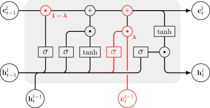
Figure 2: Schematic diagram of a CAS-LSTM block.

In this section, we give the detailed formulation of architectures used in experiments.

3.1 Stacked LSTMs

While there exist various versions of LSTM formulation, in this work we use the following, the most common variant:

$$\mathbf{i}_{t}^{l} =\sigma(\mathbf{W}_{i}^{l}\mathbf{h}_{t}^{l-1}+\mathbf{U}_{i}^{l}\mathbf{h}_{t-1}^{l}+\mathbf{b}_{i}^{l})$$ (1)

$$\mathbf{f}_{t}^{l} =\sigma(\mathbf{W}_{f}^{l}\mathbf{h}_{t}^{l-1}+\mathbf{U}_{f}^{l}\mathbf{h}_{t-1}^{l}+\mathbf{b}_{f}^{l})$$ (2)

$$\tilde{\mathbf{c}}_{t}^{l} =\tanh(\mathbf{W}_{c}^{l}\mathbf{h}_{t}^{l-1}+\mathbf{U}_{c}^{l}\mathbf{h}_{t-1}^{l}+\mathbf{b}_{c}^{l})$$ (3)

$$\mathbf{o}_{t}^{l} =\sigma(\mathbf{W}_{o}^{l}\mathbf{h}_{t}^{l-1}+\mathbf{U}_{o}^{l}\mathbf{h}_{t-1}^{l}+\mathbf{b}_{o}^{l})$$ (4)

$$\mathbf{c}_{t}^{l} =\mathbf{i}_{t}^{l}\odot\tilde{\mathbf{c}}_{t}^{l}+\mathbf{f}_{t}^{l}\odot\mathbf{c}_{t-1}^{l}$$ (5)

$$\mathbf{h}_{t}^{l} =\mathbf{o}_{t}^{l}\odot\tanh(\mathbf{c}_{t}^{l}),$$ (6)

where $t\in\{1,\cdots,T\}$ and $l\in\{1,\cdots,L\}$. $\mathbf{W}_{\cdot}^{l}\in\mathbb{R}^{d_{l}\times d_{l-1}}$, $\mathbf{U}_{\cdot}^{l}\in\mathbb{R}^{d_{l}\times d_{l}}$, $\mathbf{b}_{\cdot}^{l}\in\mathbb{R}^{d_{l}}$ are trainable parameters, and $\sigma(\cdot)$ and $\tanh(\cdot)$ are the sigmoid and the hyperbolic tangent function respectively. Also we assume that $\mathbf{h}_{t}^{0}=\mathbf{x}_{t}\in\mathbb{R}^{d_{0}}$ where $\mathbf{x}_{t}$ is the $t$-th element of an input sequence.

The input gate $\mathbf{i}_{t}^{l}$ and the forget gate $\mathbf{f}_{t}^{l}$ control the amount of information transmitted from $\tilde{\mathbf{c}}_{t}^{l}$ and $\mathbf{c}_{t-1}^{l}$, the candidate cell state and the previous cell state, to the new cell state $\mathbf{c}_{t}^{l}$. Similarly the output gate $\mathbf{o}_{t}^{l}$ soft-selects which portion of the cell state $\mathbf{c}_{t}^{l}$ is to be used in the final hidden state.

We can clearly see that the cell states $\mathbf{c}_{t-1}^{l}$, $\tilde{\mathbf{c}}_{t}^{l}$, $\mathbf{c}_{t}^{l}$ play a crucial role in forming horizontal recurrence. However the current formulation does not consider the cell state from $(l-1)$-th layer ($\mathbf{c}_{t}^{l-1}$) in computation and thus the lower context is reflected only through the rudimentary way, hindering the possibility of controlling vertical information flow.

3.2 Cell-aware Stacked LSTMs

Now we extend the stacked LSTM formulation defined above to address the problem noted in the previous subsection. To enhance the interaction between layers in a way similar to how LSTMs keep and forget the information from the previous time step, we introduce the additional forget gate $\mathbf{g}_{t}^{l}$ that determines whether to accept or ignore the signals coming from the previous layer.

The proposed Cell-aware Stacked LSTM (CAS-LSTM) architecture is defined as follows:

$$\mathbf{i}_{t}^{l} =\sigma(\mathbf{W}_{i}^{l}\mathbf{h}_{t}^{l-1}+\mathbf{U}_{i}^{l}\mathbf{h}_{t-1}^{l}+\mathbf{b}_{i}^{l})$$ (7)

$$\mathbf{f}_{t}^{l} =\sigma(\mathbf{W}_{f}^{l}\mathbf{h}_{t}^{l-1}+\mathbf{U}_{f}^{l}\mathbf{h}_{t-1}^{l}+\mathbf{b}_{f}^{l})$$ (8)

$$\mathbf{g}_{t}^{l} =\sigma(\mathbf{W}_{g}^{l}\mathbf{h}_{t}^{l-1}+\mathbf{U}_{g}^{l}\mathbf{h}_{t-1}^{l}+\mathbf{b}_{g}^{l})$$ (9)

$$\tilde{\mathbf{c}}_{t}^{l} =\tanh(\mathbf{W}_{c}^{l}\mathbf{h}_{t}^{l-1}+\mathbf{U}_{c}^{l}\mathbf{h}_{t-1}^{l}+\mathbf{b}_{c}^{l})$$ (10)

$$\mathbf{o}_{t}^{l} =\sigma(\mathbf{W}_{o}^{l}\mathbf{h}_{t}^{l-1}+\mathbf{U}_{o}^{l}\mathbf{h}_{t-1}^{l}+\mathbf{b}_{o}^{l})$$ (11)

$$\mathbf{c}_{t}^{l} =\mathbf{i}_{t}^{l}\odot{\tilde{\mathbf{c}}}_{t}^{l}+(\bm{1-\lambda})\odot\mathbf{f}_{t}^{l}\odot\mathbf{c}_{t-1}^{l}+\bm{\lambda}\odot\mathbf{g}_{t}^{l}\odot\mathbf{c}_{t}^{l-1}$$ (12)

$$\mathbf{h}_{t}^{l} =\mathbf{o}_{t}^{l}\odot\tanh(\mathbf{c}_{t}^{l}),$$ (13)

where $l>1$ and $d_{l}=d_{l-1}$. $\bm{\lambda}$ can either be a vector of constants or parameters. When $l=1$, the equations defined in the previous subsection are used. Therefore, it can be said that each non-bottom layer of CAS-LSTM accepts two sets of hidden and cell states—one from the left context and the other from the below context. The left and the below context participate in computation with the equivalent procedure so that the information from lower layers can be efficiently propagated. Fig. LABEL:fig:comparison compares CAS-LSTM to the conventional stacked LSTM architecture, and Fig. 2 depicts the computation flow of the CAS-LSTM.

We argue that considering $\mathbf{c}_{t}^{l-1}$ in computation is beneficial for the following reasons. First, contrary to $\mathbf{h}_{t}^{l-1}$, $\mathbf{c}_{t}^{l-1}$ contains information which is not filtered by $\mathbf{o}_{t}^{l-1}$. Thus a model that directly uses $\mathbf{c}_{t}^{l-1}$ does not rely solely on $\mathbf{o}_{t}^{l-1}$ for extracting information, due to the fact that it has access to the raw information $\mathbf{c}_{t}^{l-1}$, as in temporal connections. In other words, $\mathbf{o}_{t}^{l-1}$ no longer has to take all responsibility for selecting useful features for both horizontal and vertical transitions, and the burden of selecting information is shared with $\mathbf{g}_{t}^{l}$.

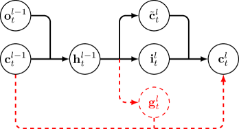
Figure 3: Visualization of paths between $\mathbf{c}_{t}^{l-1}$ and $\mathbf{c}_{t}^{l}$. In CAS-LSTM, the direct connection between $\mathbf{c}_{t}^{l-1}$ and $\mathbf{c}_{t}^{l}$ exists (denoted as red dashed lines).

Another advantage of using the $\mathbf{c}_{t}^{l-1}$ lies in the fact that it directly connects $\mathbf{c}_{t}^{l-1}$ and $\mathbf{c}_{t}^{l}$. This direct connection could help and stabilize training, since the terminal error signals can be easily backpropagated to the model parameters by the shortened propagation path. Fig. 3 illustrates paths between the two cell states.

Regarding $\bm{\lambda}$, we find experimentally that there is little difference between having it be a constant and a trainable vector bounded in $(0,1)$, and we practically find that setting $\lambda_{i}=0.5$ works well across multiple experiments. We also experimented with the architecture without $\bm{\lambda}$ i.e. two cell states are combined by unweighted summation similar to multidimensional RNNs (Graves and Schmidhuber, 2009), and found that it leads to performance degradation and unstable convergence, likely due to mismatch in the range of cell state values between layers ($(-2,2)$ for the first layer and $(-3,3)$ for the others). Experimental results on various $\bm{\lambda}$ are presented in §4.6.

3.3 Sentence Encoders

For text classification tasks, a variable-length sentence should be represented as a fixed-length vector. We describe the sentence encoder architectures used in experiments in this subsection.

First, we assume that a sequence of $T$ one-hot word vectors is given as input: $(\mathbf{w}_{1},\cdots,\mathbf{w}_{T})$, $\mathbf{w}_{t}\in\mathbb{R}^{|V|}$ where $V$ is the vocabulary set. The words are projected to corresponding word representations: $\mathbf{X}=(\mathbf{x}_{1},\cdots,\mathbf{x}_{T})$ where $\mathbf{x}_{t}=\mathbf{E}^{\top}\mathbf{w}_{t}\in\mathbb{R}^{d_{0}}$, $\mathbf{E}\in\mathbf{R}^{|V|\times d_{0}}$. Then $\mathbf{X}$ is fed to a $L$-layer CAS-LSTM model, resulting in the representations $\mathbf{H}=(\mathbf{h}_{1}^{L},\cdots,\mathbf{h}_{T}^{L})\in\mathbb{R}^{T\times d_{L}}$. The encoded sentence representation $\mathbf{s}\in\mathbb{R}^{d_{L}}$ is computed by max-pooling $\mathbf{H}$ over time as in the work of Conneau et al. (2017). Similar to their results, from preliminary experiments we found that the max-pooling performs consistently better than the mean-pooling and the last-pooling.

For better modeling of semantics, a bidirectional CAS-LSTM network may also be used. In the bidirectional case, the representations obtained by left-to-right reading $\mathbf{H}=(\mathbf{h}_{1}^{L},\cdots,\mathbf{h}_{T}^{L})\in\mathbb{R}^{T\times d_{L}}$ and those by right-to-left reading $\widehat{\mathbf{H}}=(\widehat{\mathbf{h}}_{1}^{L},\cdots,\widehat{\mathbf{h}}_{T}^{L})\in\mathbb{R}^{T\times d_{L}}$ are concatenated and max-pooled to yield the sentence representation $\mathbf{s}\in\mathbb{R}^{2d_{L}}$. We call this bidirectional architecture Bi-CAS-LSTM in experiments.

To predict the final task-specific label, we apply a task-specific feature extraction function $\phi$ to the sentence representation(s) and feed the extracted features to a classifier network. For the classifier network, a multi-layer perceptron (MLP) with the ReLU activation followed by the linear projection and the softmax function is used:

$$P(\mathbf{y}|\mathbf{X})=\text{softmax}(\mathbf{W}_{c}\text{MLP}(\phi(\cdot))),$$ (14)

where $\mathbf{W}_{c}\in\mathbb{R}^{|L|\times d_{h}}$, $|L|$ is the number of label classes, and $d_{h}$ the dimension of the MLP output.

4 Experiments

We evaluate our method on three benchmark tasks on sentence encoding: natural language inference (NLI), paraphrase identification (PI), and sentiment classification. To further demonstrate the general applicability of our method on text generation, we also evaluate the proposed method on machine translation. In addition, we conduct analysis on gate values model variations for the understanding of the architecture. We refer readers to the supplemental material for detailed experimental settings. The code will be made public for reproduction.

For the NLI and PI tasks, there exists architectures specializing in sentence pair classification. However in this work we confine our model to the architecture that encodes each sentence using a shared encoder without any inter-sentence interaction, in order to focus on the effectiveness of the architectures in extracting semantics. But note that the applicability of CAS-LSTM is not limited to sentence encoder–based approaches.

4.1 Natural Language Inference

Model	Acc. (%)	# Params
300D LSTM (Bowman et al., 2016)	80.6	3.0M
300D TBCNN (Mou et al., 2016)	82.1	3.5M
300D SPINN-PI (Bowman et al., 2016)	83.2	3.7M
600D BiLSTM with intra-attention (Liu et al., 2016)	84.2	2.8M
4096D BiLSTM with max-pooling (Conneau et al., 2017)	84.5	40M
300D BiLSTM with gated pooling (Chen et al., 2017)	85.5	12M
300D Gumbel Tree-LSTM (Choi et al., 2018b)	85.6	2.9M
600D Shortcut stacked BiLSTM (Nie and Bansal, 2017)	86.1	140M
300D Reinforced self-attention network (Shen et al., 2018)	86.3	3.1M
600D BiLSTM with generalized pooling (Chen et al., 2018)	86.6	65M
300D 2-layer CAS-LSTM (ours)	86.4	2.9M
300D 2-layer Bi-CAS-LSTM (ours)	86.8	6.8M
300D 3-layer CAS-LSTM (ours)	86.4	4.8M
300D 3-layer Bi-CAS-LSTM (ours)	87.0	8.6M

Table 1: Results of the models on the SNLI dataset.

Model	In (%)	Cross (%)	# Params
CBOW (Williams et al., 2018b)	64.8	64.5	-
BiLSTM (Williams et al., 2018b)	66.9	66.9	-
Shortcut stacked BiLSTM (Nie and Bansal, 2017)∗	74.6	73.6	140M
BiLSTM with gated pooling (Chen et al., 2017)	73.5	73.6	12M
BiLSTM with generalized pooling (Chen et al., 2018)	73.8	74.0	18M∗∗
2-layer CAS-LSTM (ours)	74.0	73.3	2.9M
2-layer Bi-CAS-LSTM (ours)	74.6	73.7	6.8M
3-layer CAS-LSTM (ours)	73.8	73.1	4.8M
3-layer Bi-CAS-LSTM (ours)	74.2	73.4	8.6M

Table 2: Results of the models on the MultiNLI dataset. ‘In’ and ‘Cross’ represent accuracy calculated from the matched and mismatched test set respectively. ^∗: SNLI dataset is used as additional training data. ^∗∗: computed from hyperparameters provided by the authors.

For the evaluation of performance of the proposed method on the NLI task, SNLI (Bowman et al., 2015) and MultiNLI (Williams et al., 2018b) datasets are used. The objective of both datasets is to predict the relationship between a premise and a hypothesis sentence: entailment, contradiction, and neutral. SNLI and MultiNLI datasets are composed of about 570k and 430k premise-hypothesis pairs respectively.

GloVe pretrained word embeddings (Pennington et al., 2014) are used and remain fixed during training. The dimension of encoder states ($d_{l}$) is set to 300 and a 1024D MLP with one or two hidden layers is used. We apply dropout (Srivastava et al., 2014) to the word embeddings and the MLP layers. The features used as input to the MLP classifier are extracted by the following equation:

$$\phi(\mathbf{s}_{1},\mathbf{s}_{2})=\mathbf{s}_{1}\oplus\mathbf{s}_{2}\oplus|\mathbf{s}_{1}-\mathbf{s}_{2}|\oplus(\mathbf{s}_{1}\odot\mathbf{s}_{2}),$$ (15)

where $\oplus$ is the vector concatenation operator.

Table 1 and 2 contain results of the models on SNLI and MultiNLI datasets. Along with other state-of-the-art models, the tables include several stacked LSTM–based models to facilitate comparison of our work with prior related work. Liu et al. (2016); Chen et al. (2017, 2018) adopt advanced pooling algorithms motivated by the attention mechanism to obtain a fixed-length sentence vector. Nie and Bansal (2017) use the concatenation of all outputs from previous layers as input to the next layer.

In SNLI, our best model achieves the accuracy of 87.0%, which is the new state-of-the-art among the sentence encoder–based models, with relatively fewer parameters. Similarly in MultiNLI, our models match the accuracy of state-of-the-art models in both in-domain (matched) and cross-domain (mismatched) test sets. Note that only the GloVe word vectors are used as word representations, as opposed to some models that introduce character-level features. It is also notable that our proposed architecture does not restrict the selection of pooling method; the performance could further be improved by replacing max-pooling with other advanced algorithms e.g. intra-sentence attention (Liu et al., 2016) and generalized pooling (Chen et al., 2018).

4.2 Paraphrase Identification

Model	Acc. (%)
CNN (Wang et al., 2017)	79.6
LSTM (Wang et al., 2017)	82.6
Multi-Perspective LSTM (Wang et al., 2017)	83.2
LSTM + ElBiS (Choi et al., 2018a)	87.3
REGMAPR (BASE+REG) (Brahma, 2018)	88.0
CAS-LSTM (ours)	88.4
Bi-CAS-LSTM (ours)	88.6

Table 3: Results of the models on the Quora Question Pairs dataset.

We use Quora Question Pairs dataset (Wang et al., 2017) in evaluating the performance of our method on the PI task. The dataset consists of over 400k question pairs, and each pair is annotated with whether the two sentences are paraphrase of each other or not.

Similarly to the NLI experiments, GloVe pretrained vectors, 300D encoders, and 1024D MLP are used. The number of CAS-LSTM layers is fixed to 2 in PI experiments. Two sentence vectors are aggregated using the following equation and fed as input to the classifier.

$$\phi(\mathbf{s}_{1},\mathbf{s}_{2})=|\mathbf{s}_{1}-\mathbf{s}_{2}|\oplus(\mathbf{s}_{1}\odot\mathbf{s}_{2})$$ (16)

The results on the Quora Question Pairs dataset are summarized in Table 3. Again we can see that our models outperform other models, especially compared to conventional LSTM–based models. Also note that Multi-Perspective LSTM (Wang et al., 2017), LSTM + ElBiS (Choi et al., 2018a), and REGMAPR (BASE+REG) (Brahma, 2018) in Table 3 are approaches that focus on designing a more sophisticated function for aggregating two sentence vectors, and their aggregation functions could be also applied to our work for further improvement.

4.3 Sentiment Classification

Model	SST-2 (%)	SST-5 (%)
Recursive Neural Tensor Network (Socher et al., 2013)	85.4	45.7
2-layer LSTM (Tai et al., 2015)	86.3	46.0
2-layer BiLSTM (Tai et al., 2015)	87.2	48.5
Constituency Tree-LSTM (Tai et al., 2015)	88.0	51.0
Constituency Tree-LSTM with recurrent dropout (Looks et al., 2017)	89.4	52.3
byte mLSTM (Radford et al., 2017)∗	91.8	52.9
Gumbel Tree-LSTM (Choi et al., 2018b)	90.7	53.7
BCN + Char + ELMo (Peters et al., 2018)∗	-	54.7
2-layer CAS-LSTM (ours)	91.1	53.0
2-layer Bi-CAS-LSTM (ours)	91.3	53.6

Table 4: Results of the models on the SST dataset. ^∗: models pretrained on large external corpora are used.

In evaluating sentiment classification performance, the Stanford Sentiment Treebank (SST) (Socher et al., 2013) is used. It consists of about 12,000 binary-parsed sentences where constituents (phrases) of each parse tree are annotated with a sentiment label (very positive, positive, neutral, negative, very negative). Following the convention of prior work, all phrases and their labels are used in training but only the sentence-level data are used in evaluation.

In evaluation we consider two settings, namely SST-2 and SST-5, the two differing only in their level of granularity with regard to labels. In SST-2, data samples annotated with ‘neutral’ are ignored from training and evaluation. The two positive labels (very positive, positive) are considered as the same label, and similarly for the two negative labels. As a result 98,794/872/1,821 data samples are used in training/validation/test, and the task is considered as a binary classification problem. In SST-5, all 318,582/1,101/2,210 data samples are used and the task is a 5-class classification problem.

Since the task is a single-sentence classification problem, we use the sentence representation itself as input to the classifier. We use 300D GloVe vectors, 2-layer 150D or 300D encoders, and a 300D MLP classifier for the models, however unlike previous experiments we tune the word embeddings during training. The results on SST are listed in Table 4. Our models clearly outperform plain LSTM- and BiLSTM-based models, and are competitive to other state-of-the-art models, without utilizing parse tree information.

4.4 Machine Translation

Model	BLEU
256D LSTM	28.1 $\pm$ 0.22
256D CAS-LSTM	28.8 $\pm$ 0.04∗
247D CAS-LSTM	28.7 $\pm$ 0.07∗

Table 5: Results of the models on the IWSLT 2014 de-en dataset. ^∗: $p<0.0005$ (one-tailed paired t-test).

We use the IWSLT 2014 machine evaluation campaign dataset (Cettolo et al., 2014) in machine translation experiments. We used the fairseq library (Gehring et al., 2017) for experiments. Moses tokenizer is used for word tokenization and the byte pair encoding (Sennrich et al., 2016) is applied to confine the size of the vocabulary set up to 10,000.

Similar to Wiseman and Rush (2016), a 2-layer 256D sequence-to-sequence LSTM model with the attentional decoder is used as baseline, and we replace the encoder and the decoder network with the proposed architecture for the evaluation of performance improvement. For decoding, beam search with $B=10$ is used. For fair comparison, we tune hyperparameters for all models based on the performance on the validation dataset and train the same model for five times with different random seeds. Also, to cancel out the increased number of parameters, we experiment with the 247D CAS-LSTM model which has the roughly same number of parameters as the baseline model (8.2M).

From Table 5, we can see that the CAS-LSTM models bring significant performance gains over the baseline model.

4.5 Forget Gate Analysis

To inspect the effect of the additional forget gate, we investigate how the values of vertical forget gates are distributed. We sample 1,000 random sentences from the development set of the SNLI dataset, and use the 3-layer CAS-LSTM model trained on the SNLI dataset to compute gate values.

If all values from a vertical forget gate $\mathbf{g}_{t}^{l}$ were to be 0, this would mean that the introduction of the additional forget gate is meaningless and the model would reduce to a plain stacked LSTM. On the contrary if all values were 1, meaning that the vertical forget gates were always open, it would be impossible to say that the information is modulated effectively.

Fig. LABEL:fig:gate-a and LABEL:fig:gate-b represent histograms of the vertical forget gate values from the second and the third layer. From the figures we can validate that the trained model does not fall into the degenerate case where vertical forget gates are ignored. Also the figures show that the values are right-skewed, which we conjecture to be a result of focusing more on a strong interaction between adjacent layers.

To further verify that the gate values are diverse enough within each time step, we compute the distribution of the range of values per time step, $R(\mathbf{g}_{t}^{l})=\max_{i}{g_{t,i}^{l}}-\min_{i}{{g}_{t,i}^{l}}$, where $\mathbf{g}_{t}^{l}=[g_{t,1}^{l},\cdots,g_{t,d_{l}}^{l}]^{\top}$. We plot the histograms in Fig. LABEL:fig:gate-c and LABEL:fig:gate-d. From the figures we see that the vertical forget gate controls the amount of information flow effectively, making diverse decisions of retaining or discarding signals across dimensions.

Finally, to investigate the argument presented in §3 that the additional forget gate helps the previous output gate with reducing the burden of extracting all needed information, we inspect the distribution of the values from $|\mathbf{g}_{t}^{l}-\mathbf{o}_{t}^{l-1}|$. This distribution indicates how differently the vertical forget gate and the previous output gate select information from $\mathbf{c}_{t}^{l-1}$. From Fig. LABEL:fig:gate-e and LABEL:fig:gate-f we can see that the two gates make fairly different decisions, from which we demonstrate that the direct path between $\mathbf{c}_{t}^{l-1}$ and $\mathbf{c}_{t}^{l}$ enables a model to utilize signals overlooked by $\mathbf{o}_{t}^{l-1}$.

4.6 Model Variations

In this subsection, we see the influence of each component of a model on performance by removing or replacing its components. the SNLI dataset is used for experiments, and the best performing configuration is used as a baseline for modifications. We consider the following variants: (i) models with different $\bm{\lambda}$, (ii) models without $\bm{\lambda}$, and (iii) models that integrate lower contexts via peephole connections.

Variant (iii) calculates and applies the forget gate $\mathbf{g}_{t}^{l}$ which takes charge of integrating lower contexts via the equations below, following the work of Zhang et al. (2016):

$$\begin{split}\mathbf{g}_{t}^{l}&=\sigma(\mathbf{W}_{g}^{l}\mathbf{h}_{t}^{l-1}+\mathbf{p}_{g_{1}}^{l}\odot\mathbf{c}_{t-1}^{l}+\mathbf{p}_{g_{2}}^{l}\odot\mathbf{c}_{t}^{l-1}+\mathbf{b}_{g}^{l})\end{split}$$ (17)

$$\mathbf{c}_{t}^{l} =\mathbf{i}_{t}^{l}\odot\tilde{\mathbf{c}}_{t}^{l}+\mathbf{f}_{t}^{l}\odot\mathbf{c}_{t-1}^{l}+\mathbf{g}_{t}^{l}\odot\mathbf{c}_{t}^{l-1},$$ (18)

where $\mathbf{p}_{\cdot}^{l}\in\mathbb{R}^{d_{l}}$ represent peephole weight vectors that take cell states into account. We can see that the computation formulae of $\mathbf{f}_{t}^{l}$ and $\mathbf{g}_{t}^{l}$ are not consistent, in that $\mathbf{h}_{t-1}^{l}$ does not participate in computing $\mathbf{g}_{t-1}^{l}$, and that the left and the below context are reflected in $\mathbf{g}_{t-1}^{l}$ only via element-wise multiplications which do not consider the interaction among dimensions. By contrast, ours uses the analogous formulae in calculating $\mathbf{f}_{t}^{l}$ and $\mathbf{g}_{t}^{l}$, considers $\mathbf{h}_{t-1}^{l}$ in calculating $\mathbf{g}_{t}^{l}$, and introduces the scaling factor $\bm{\lambda}$.

Table 6 summarizes the results of model variants. From the results of baseline and (i), we validate that the selection of $\bm{\lambda}$ does not significantly affect performance but introducing $\bm{\lambda}$ is beneficial (baseline vs. (ii)) possibly due to its effect on normalizing information from multiple sources, as mentioned in §3. Also, from the comparison between baseline and (iii), we show that the proposed way of combining the left and the lower contexts leads to better modeling of sentence representations than that of Zhang et al. (2016).

Model	Acc. (%)	$\Delta$
Bi-CAS-LSTM (baseline)	87.0
(i) Diverse $\bm{\lambda}$
(a) $\lambda_{i}=0.25$	86.8	-0.2
(b) $\lambda_{i}=0.75$	86.8	-0.2
(c) Trainable $\bm{\lambda}$	86.9	-0.1
(ii) No $\bm{\lambda}$	86.6	-0.4
(iii) Integration through peepholes	86.5	-0.5

Table 6: Results of model variants.

5 Conclusion

In this paper, we proposed a method of stacking multiple LSTM layers for modeling sentences, dubbed CAS-LSTM. It uses not only hidden states but also cell states from the previous layer, for the purpose of controlling the vertical information flow in a more elaborate way. We evaluated the proposed method on various benchmark tasks: natural language inference, paraphrase identification, and sentiment classification. Our models outperformed plain LSTM-based models in all experiments and were competitive other state-of-the-art models. The proposed architecture can replace any stacked LSTM only under one weak restriction—the size of states should be identical across all layers.

For future work we plan to apply the CAS-LSTM architecture beyond sentence modeling tasks. Various problems such as sequence labeling and language modeling might benefit from sophisticated modulation on context integration. Aggregating diverse contexts from sequential data, e.g. those from forward and backward reading of text, could also be an intriguing research direction.

References

- Bahdanau et al. (2015) Dzmitry Bahdanau, Kyunghyun Cho, and Yoshua Bengio. Neural machine translation by jointly learning to align and translate. In ICLR, 2015.
- Bowman et al. (2015) Samuel R. Bowman, Gabor Angeli, Christopher Potts, and Christopher D. Manning. A large annotated corpus for learning natural language inference. In EMNLP, pages 632–642, 2015.
- Bowman et al. (2016) Samuel R. Bowman, Jon Gauthier, Abhinav Rastogi, Raghav Gupta, Christopher D. Manning, and Christopher Potts. A fast unified model for parsing and sentence understanding. In ACL, pages 1466–1477, 2016.
- Brahma (2018) Siddhartha Brahma. REGMAPR - A recipe for textual matching. CoRR, cs.CL/1808.04343v1, 2018.
- Cettolo et al. (2014) Mauro Cettolo, Jan Niehues, Sebastian Stüker, Luisa Bentivogli, and Marcello Federico. Report on the 11th IWSLT evaluation campaign. In IWSLT, 2014.
- Chen et al. (2017) Qian Chen, Xiaodan Zhu, Zhen-Hua Ling, Si Wei, Hui Jiang, and Diana Inkpen. Recurrent neural network-based sentence encoder with gated attention for natural language inference. In RepEval, pages 36–40, 2017.
- Chen et al. (2018) Qian Chen, Zhen-Hua Ling, and Xiaodan Zhu. Enhancing sentence embedding with generalized pooling. In COLING, pages 1815–1826, 2018.
- Cho et al. (2014) Kyunghyun Cho, Bart van Merrienboer, Caglar Gulcehre, Dzmitry Bahdanau, Fethi Bougares, Holger Schwenk, and Yoshua Bengio. Learning phrase representations using RNN encoder–decoder for statistical machine translation. In EMNLP, pages 1724–1734, 2014.
- Choi et al. (2018a) Jihun Choi, Taeuk Kim, and Sang-goo Lee. Element-wise bilinear interaction for sentence matching. In *SEM, pages 107–112, 2018a.
- Choi et al. (2018b) Jihun Choi, Kang Min Yoo, and Sang-goo Lee. Learning to compose task-specific tree structures. In AAAI, pages 5094–5101, 2018b.
- Conneau et al. (2017) Alexis Conneau, Douwe Kiela, Holger Schwenk, Loïc Barrault, and Antoine Bordes. Supervised learning of universal sentence representations from natural language inference data. In EMNLP, pages 670–680, 2017.
- Dyer et al. (2016) Chris Dyer, Adhiguna Kuncoro, Miguel Ballesteros, and Noah A. Smith. Recurrent neural network grammars. In NAACL-HLT, pages 199–209, 2016.
- El Hihi and Bengio (1996) Salah El Hihi and Yoshua Bengio. Hierarchical recurrent neural networks for long-term dependencies. In NIPS, pages 493–499, 1996.
- Elman (1990) Jeffrey L. Elman. Finding structure in time. Cognitive Science, 14(2):179–211, 1990.
- Gehring et al. (2017) Jonas Gehring, Michael Auli, David Grangier, Denis Yarats, and Yann N. Dauphin. Convolutional sequence to sequence learning. In ICML, pages 1243–1252, 2017.
- Goller and Kuchler (1996) Christoph Goller and Andreas Kuchler. Learning task-dependent distributed representations by backpropagation through structure. In ICNN, pages 347–352, 1996.
- Goodfellow et al. (2016) Ian Goodfellow, Yoshua Bengio, and Aaron Courville. Deep Learning. MIT Press, 2016.
- Graves (2013) Alex Graves. Generating sequences with recurrent neural networks. CoRR, cs.NE/1308.0850v5, 2013.
- Graves and Schmidhuber (2009) Alex Graves and Jürgen Schmidhuber. Offline handwriting recognition with multidimensional recurrent neural networks. In NIPS, pages 545–552, 2009.
- Graves et al. (2007) Alex Graves, Santiago Fernández, and Jürgen Schmidhuber. Multi-dimensional recurrent neural networks. In ICANN, pages 549–558, 2007.
- Hermans and Schrauwen (2013) Michiel Hermans and Benjamin Schrauwen. Training and analysing deep recurrent neural networks. In NIPS, pages 190–198, 2013.
- Hochreiter and Schmidhuber (1997) Sepp Hochreiter and Jürgen Schmidhuber. Long short-term memory. Neural Computation, 9(8):1735–1780, 1997.
- Kalchbrenner et al. (2016) Nal Kalchbrenner, Ivo Danihelka, and Alex Graves. Grid long short-term memory. In ICLR, 2016.
- Kim et al. (2017) Jaeyoung Kim, Mostafa El-Khamy, and Jungwon Lee. Residual LSTM: Design of a deep recurrent architecture for distant speech recognition. In INTERSPEECH, pages 1591–1595, 2017.
- Kiperwasser and Goldberg (2016) Eliyahu Kiperwasser and Yoav Goldberg. Simple and accurate dependency parsing using bidirectional LSTM feature representations. Transactions of the Association for Computational Linguistics, 4:313–327, 2016.
- Le and Zuidema (2015) Phong Le and Willem Zuidema. Compositional distributional semantics with long short term memory. In *SEM, pages 10–19, 2015.
- Liu et al. (2016) Yang Liu, Chengjie Sun, Lei Lin, and Xiaolong Wang. Learning natural language inference using bidirectional LSTM model and inner-attention. CoRR, cs.CL/1605.09090v1, 2016.
- Looks et al. (2017) Moshe Looks, Marcello Herreshoff, DeLesley Hutchins, and Peter Norvig. Deep learning with dynamic computation graphs. In ICLR, 2017.
- Mikolov et al. (2010) Tomáš Mikolov, Martin Karafiát, Lukáš Burget, Jan Černockỳ, and Sanjeev Khudanpur. Recurrent neural network based language model. In INTERSPEECH, pages 1045–1048, 2010.
- Mou et al. (2016) Lili Mou, Rui Men, Ge Li, Yan Xu, Lu Zhang, Rui Yan, and Zhi Jin. Natural language inference by tree-based convolution and heuristic matching. In ACL, pages 130–136, 2016.
- Nie and Bansal (2017) Yixin Nie and Mohit Bansal. Shortcut-stacked sentence encoders for multi-domain inference. In RepEval, pages 41–45, 2017.
- Pascanu et al. (2014) Razvan Pascanu, Caglar Gulcehre, Kyunghyun Cho, and Yoshua Bengio. How to construct deep recurrent neural networks. In ICLR, 2014.
- Pennington et al. (2014) Jeffrey Pennington, Richard Socher, and Christopher Manning. GloVe: Global vectors for word representation. In EMNLP, pages 1532–1543, 2014.
- Peters et al. (2018) Matthew Peters, Mark Neumann, Mohit Iyyer, Matt Gardner, Christopher Clark, Kenton Lee, and Luke Zettlemoyer. Deep contextualized word representations. In NAACL-HLT, pages 2227–2237, 2018.
- Radford et al. (2017) Alec Radford, Rafal Jozefowicz, and Ilya Sutskever. Learning to generate reviews and discovering sentiment. CoRR, cs.LG/1704.01444v2, 2017.
- Schmidhuber (1992) Jürgen Schmidhuber. Learning complex, extended sequences using the principle of history compression. Neural Computation, 4(2):234–242, 1992.
- Sennrich et al. (2016) Rico Sennrich, Barry Haddow, and Alexandra Birch. Neural machine translation of rare words with subword units. In ACL, pages 1715–1725, 2016.
- Shen et al. (2018) Tao Shen, Tianyi Zhou, Guodong Long, Jing Jiang, Sen Wang, and Chengqi Zhang. Reinforced self-attention network: A hybrid of hard and soft attention for sequence modeling. In IJCAI, pages 4345–4352, 2018.
- Shi et al. (2018) Haoyue Shi, Hao Zhou, Jiaze Chen, and Lei Li. On tree-based neural sentence modeling. In EMNLP, pages 4631–4641, 2018.
- Socher et al. (2011) Richard Socher, Cliff Chiung-Yu Lin, Andrew Y. Ng, and Christopher D. Manning. Parsing natural scenes and natural language with recursive neural networks. In ICML, pages 129–136, 2011.
- Socher et al. (2013) Richard Socher, Alex Perelygin, Jean Wu, Jason Chuang, Christopher D. Manning, Andrew Ng, and Christopher Potts. Recursive deep models for semantic compositionality over a sentiment treebank. In EMNLP, pages 1631–1642, 2013.
- Srivastava et al. (2014) Nitish Srivastava, Geoffrey Hinton, Alex Krizhevsky, Ilya Sutskever, and Ruslan Salakhutdinov. Dropout: A simple way to prevent neural networks from overfitting. Journal of Machine Learning Research, 15:1929–1958, 2014.
- Sutskever (2013) Ilya Sutskever. Training recurrent neural networks. PhD thesis, University of Toronto, 2013.
- Sutskever et al. (2014) Ilya Sutskever, Oriol Vinyals, and Quoc V. Le. Sequence to sequence learning with neural networks. In NIPS, pages 3104–3112, 2014.
- Tai et al. (2015) Kai Sheng Tai, Richard Socher, and Christopher D. Manning. Improved semantic representations from tree-structured long short-term memory networks. In ACL-IJCNLP, pages 1556–1566, 2015.
- Tang et al. (2015) Duyu Tang, Bing Qin, and Ting Liu. Document modeling with gated recurrent neural network for sentiment classification. In EMNLP, pages 1422–1432, 2015.
- Tran et al. (2017) Quan Tran, Andrew MacKinlay, and Antonio Jimeno Yepes. Named entity recognition with stack residual LSTM and trainable bias decoding. In IJCNLP, pages 566–575, 2017.
- Wang et al. (2017) Zhiguo Wang, Wael Hamza, and Radu Florian. Bilateral multi-perspective matching for natural language sentences. In IJCAI, pages 4144–4150, 2017.
- Williams et al. (2018a) Adina Williams, Andrew Drozdov, and Samuel R. Bowman. Do latent tree learning models identify meaningful structure in sentences? Transactions of the Association for Computational Linguistics, 6:253–267, 2018a.
- Williams et al. (2018b) Adina Williams, Nikita Nangia, and Samuel Bowman. A broad-coverage challenge corpus for sentence understanding through inference. In NAACL-HLT, pages 1112–1122, 2018b.
- Wiseman and Rush (2016) Sam Wiseman and Alexander M. Rush. Sequence-to-sequence learning as beam-search optimization. In EMNLP, pages 1296–1306, 2016.
- Yao et al. (2015) Kaisheng Yao, Trevor Cohn, Katerina Vylomova, Kevin Duh, and Chris Dyer. Depth-gated LSTM. CoRR, cs.NE/1508.03790v4, 2015.
- Yogatama et al. (2017) Dani Yogatama, Phil Blunsom, Chris Dyer, Edward Grefenstette, and Wang Ling. Learning to compose words into sentences with reinforcement learning. In ICLR, 2017.
- Zhang et al. (2016) Yu Zhang, Guoguo Chen, Dong Yu, Kaisheng Yao, Sanjeev Khudanpur, and James Glass. Highway long short-term memory RNNs for distant speech recognition. In ICASSP, pages 5755–5759, 2016.
- Zhou et al. (2015) Chunting Zhou, Chonglin Sun, Zhiyuan Liu, and Francis Lau. A C-LSTM neural network for text classification. CoRR, cs.CL/1511.08630v2, 2015.
- Zhu et al. (2015) Xiaodan Zhu, Parinaz Sobihani, and Hongyu Guo. Long short-term memory over recursive structures. In ICML, pages 1604–1612, 2015.