Energy quantization at the three-quarter Dirac point in a magnetic field

Abstract

The quantization of the energy in a magnetic field (Landau quantization) at a three-quarter Dirac point is studied theoretically. The three-quarter Dirac point is realized in the system of massless Dirac fermions with the critically tilted Dirac cone in one direction, where a linear term disappears and a quadratic term $\alpha_{2}q_{x}^{2}$ with a constant $\alpha_{2}$ plays an important role. The energy is obtained as $E_{n}\propto\alpha_{2}^{\frac{3}{5}}(nB)^{\frac{4}{5}}$, where $n=1,2,3,\dots$, by means of numerically solving the differential equation. The same result is obtained analytically by adopting an approximation. The result is consistent with the semiclassical quantization rule studied previously. The existence of the $n=0$ state is studied by introducing the energy gap due to the inversion-symmetry-breaking term, and it is obtained that the $n=0$ state exists in one of a pair of three-quarter Dirac points, depending on the direction of the magnetic field when the energy gap is finite.

I Introduction

Massless Dirac fermions are observed in condensed matter physics, in graphene Novoselov et al. (2005); Zhang et al. (2005), organic conductorsTajima et al. (2000); Katayama et al. (2006); Kajita et al. (2014), and the surface of the 3D topological insulatorsFu et al. (2007); Hsieh et al. (2009).

When a two-dimensional system has an inversion symmetry and a time reversal symmetry, massless Dirac points ($\pm\mathbf{k}_{\textrm{D}}$) appear as a pair. The minimal model for the massless Dirac fermions is written asKobayashi et al. (2007); Goerbig et al. (2008); Kobayashi et al. (2009)

$$\mathcal{H}_{\mathrm{D}}=\begin{pmatrix}w_{0x}q_{x}+w_{0y}q_{y}&w_{x}q_{x}\mp iw_{y}q_{y}\\ w_{x}q_{x}\pm iw_{y}q_{y}&w_{0x}q_{x}+w_{0y}q_{y}\end{pmatrix},$$ (1)

where

$$\mathbf{q}=\mathbf{k}\mp\mathbf{k}_{\textrm{D}}.$$ (2)

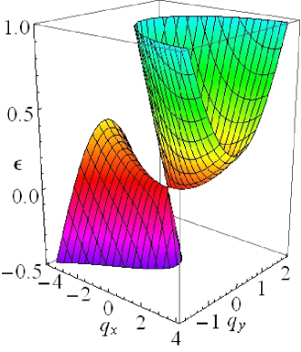
Figure 1: (Color online) Energy as a function of $q_{x}$ and $q_{y}$ at $B=0$ at the three-quarter Dirac point. Parameters are $w_{x}=0.4$, $w_{y}=1$, $w_{0x}=-w_{x}$, $w_{0y}=0$, $\alpha_{2}^{\prime}=\alpha_{2}^{\prime\prime}=0.01$,

Two bands touch at the Dirac points. When $w_{0x}=0$ and $w_{0y}=0$, the linear energy dispersion near the Dirac point (Dirac cone) is not tilted. By the finite $w_{0x}$ or $w_{0y}$, the Dirac cone is tilted, and if the condition

$$\left(\frac{w_{0x}}{w_{x}}\right)^{2}+\left(\frac{w_{0y}}{w_{y}}\right)^{2}=1,$$ (3)

is fulfilled, the Dirac cone is critically tilted, i.e., the conical edge of the Dirac cone is horizontal in one direction. In that case we have to take into account the quadratic terms in the tilted direction, except for the special case that the quadratic terms vanish by symmetry or by accident. Generally the quadratic terms exist as we have found previouslyKishigi and Hasegawa (2017) in the tight-binding model with pressure-dependent hoppings for the organic conductor, $\alpha$-(BEDT-TTF)₂I₃. The energy near the critically tilted Dirac point is shown in Fig. 1. Since the energy of the upper band depends linearly in three directions (for example, $-q_{x}$ and $\pm q_{y}$) and quadratically in one direction (for example, $+q_{x}$) in that case, we call the critically tilted Dirac point as the “three-quarter Dirac point”.Kishigi and Hasegawa (2017) It has been known that when two-Dirac points merge at the time-reversal-invariant momentum, the energy depends linearly in two directions and quadratically in two directions, and it is called the semi-Dirac pointHasegawa et al. (2006); Dietl et al. (2008); Montambaux et al. (2009); Banerjee et al. (2009); Delplace and Montambaux (2010).

Previously we have shown that the energy in a magnetic field (the Landau level) at the three-quarter Dirac point depends on the quantum number $n$ and the magnetic field $B$ as

$$\epsilon_{n}\propto(nB)^{\frac{4}{5}},$$ (4)

by calculating the energy of the tight-binding model for $\alpha$-(BEDT-TTF)₂I₃ in a magnetic field numericallyKishigi and Hasegawa (2017). In that paper we have explained these $n$ and $B$ dependences of Landau levels by using the semi-classical quantization rule. In this paper we study the Landau quantization at the three-quarter Dirac point in a numerical study and an analytical treatment with a crude approximation. The Dirac cone is taken to be critically tilted in the $k_{x}$ direction, i.e., $w_{0x}=-w_{x}$, and $w_{0y}=0$ in Eq. (1). For simplicity we take $w_{x}>0$, $w_{y}>0$, and we introduce the quadratic terms in the $q_{x}$ direction ($\alpha_{2}^{\prime}q_{x}^{2}$ in diagonal elements and $\alpha_{2}^{\prime\prime}q_{x}^{2}$ in off-diagonal elements). Then the three-quarter Dirac Hamiltonian we study in this paper is

$$\mathcal{H}_{\mathrm{tqD}}=\begin{pmatrix}-w_{x}q_{x}+\alpha_{2}^{\prime}q_{x}^{2}&w_{x}q_{x}+\alpha_{2}^{\prime\prime}q_{x}^{2}-iw_{y}q_{y}\\ w_{x}q_{x}+\alpha_{2}^{\prime\prime}q_{x}^{2}+iw_{y}q_{y}&-w_{x}q_{x}+\alpha_{2}^{\prime}q_{x}^{2}\end{pmatrix}.$$ (5)

II three-quarter Dirac point

II.1 energy at $B=0$

In the absence of the magnetic field the energy is obtained by

$$\mathcal{H}_{\mathrm{tqD}}\Psi=E(\mathbf{q})\Psi,$$ (6)

where $\Psi$ is a wave function which has two components, $\psi_{1}$ and $\Psi_{2}$. The eigenvalues of $\mathcal{H}_{\mathrm{tqD}}$ is obtained as $E(\mathbf{q})=\varepsilon^{0}_{\mathrm{tqD}_{\pm}}(\mathbf{q})$;

$$\varepsilon^{0}_{\textrm{tqD}_{\pm}}(\mathbf{q})= -w_{x}q_{x}+\alpha_{2}^{\prime}q_{x}^{2}$$

$$\pm\sqrt{(w_{x}q_{x}+\alpha_{2}^{\prime\prime}q_{x}^{2})^{2}+(w_{y}q_{y})^{2}},$$ (7)

which are plotted in Fig. 1. There exist the upper band ($\varepsilon^{0}_{\textrm{tqD}_{+}}(\mathbf{q})$) and the lower band ($\varepsilon^{0}_{\textrm{tqD}_{-}}(\mathbf{q})$). These two bands touch at $\mathbf{q}=(0,0)$. Along the $q_{x}$ axis, the linear term disappears in $\varepsilon^{0}_{\textrm{tqD}_{+}}(\mathbf{q})$ and $\varepsilon^{0}_{\textrm{tqD}_{-}}(\mathbf{q})$ for $q_{x}>0$ and $q_{x}<0$, respectively, whereas in other three directions the linear term exists;

$$\varepsilon_{\textrm{tqD}_{+}}(q_{x},q_{y}=0) =\left\{\begin{array}[]{ll}\alpha_{2}q_{x}^{2}&\mbox{ if $q_{x}>0$}\\ 2w_{x}|q_{x}|+\tilde{\alpha}_{2}q_{x}^{2}&\mbox{ if $q_{x}<0$}\end{array}\right.$$ (10)

$$\varepsilon_{\textrm{tqD}_{+}}(q_{x}=0,q_{y}) =w_{y}|q_{y}|$$ (11)

$$\varepsilon_{\textrm{tqD}_{-}}(q_{x},q_{y}=0) =\left\{\begin{array}[]{ll}-2w_{x}q_{x}+\tilde{\alpha}_{2}q_{x}^{2}&\mbox{ if $q_{x}>0$}\\ \alpha_{2}q_{x}^{2}&\mbox{ if $q_{x}<0$}\end{array}\right.$$ (14)

$$\varepsilon_{\textrm{tqD}_{-}}(q_{x}=0,q_{y}) =-w_{y}|q_{y}|,$$ (15)

where

$$\alpha_{2}=\alpha_{2}^{\prime}+|\alpha_{2}^{\prime\prime}|,$$ (16)

and

$$\tilde{\alpha}_{2}=\alpha_{2}^{\prime}-|\alpha_{2}^{\prime\prime}|.$$ (17)

If $\alpha_{2}>0$, $\mathbf{q}=0$ is a local minimum of $\varepsilon_{\textrm{tqD}_{+}}$ with the linear dispersion in three directions ($q_{x}<0$, $q_{y}>0$ and $q_{y}<0$) and quadratic dispersion in one direction ($q_{x}>0$). Note that the three-quarter Dirac point is neither the local maximum nor the local minimum of $\varepsilon_{\textrm{tqD}_{-}}$ if $\alpha_{2}>0$. If $\alpha_{2}<0$, the three-quarter Dirac point is the local maximum of $\varepsilon_{\textrm{tqD}_{-}}$, but it is neither the local maximum nor the local minimum of $\varepsilon_{\textrm{tqD}_{+}}$.

II.2 numerical results of the energy at $B>0$, using boundary condition at $y>0$

Hereafter we study the case $\alpha_{2}>0$, i.e., the three-quarter Dirac point is the minimum of $\varepsilon^{0}_{\mathrm{tqD}_{+}}$, as shown in Fig. 1. In this case it is expected that when the magnetic field is applied, there are the almost-localized bound states (the Landau levels) at $E>0$, since there exists a closed Fermi surface at $E>0$ in the $\varepsilon^{0}_{\mathrm{tqD}_{+}}$ band, and the semiclassical Landau quantization is expected for the closed orbit. On the other hand, the Fermi surface in the $\varepsilon^{0}_{\mathrm{tqD}_{-}}$ band is open and a continuous energy is expected in the $\varepsilon^{0}_{\mathrm{tqD}_{-}}$ band even in the presence of the magnetic field. Quantum mechanically the Landau levels in the $\varepsilon^{0}_{\mathrm{tqD}_{+}}$ band couple to the continuous energy in the $\varepsilon^{0}_{\mathrm{tqD}_{-}}$ band by quantum tunneling. In this subsection we show that the coupling between the almost-localized Landau levels and the continuous energy cannot be neglected for the quantized energy with the small quantum number, $n$, but it becomes small for the larger values of $n$.

In the presence of the magnetic field $\mathbf{B}$ ($\mathbf{B}=\nabla\times\mathbf{A}$, where $\mathbf{A}$ is the vector potential), we replace $q_{x}$ and $q_{y}$ as

$$q_{x} \rightarrow-i\hbar\frac{\partial}{\partial x}+eA_{x},$$ (18)

$$q_{y} \rightarrow-i\hbar\frac{\partial}{\partial y}+eA_{y}.$$ (19)

We study the case that the uniform magnetic field $B>0$ is applied along the $z$ direction. We take the vector potential as

$$\mathbf{A}=(-By,0,0).$$ (20)

Since there is no explicit $x$ in Eq. (6), we can write

$$\Psi(x,y)=e^{ik_{x}x}\begin{pmatrix}\Psi_{1}(y)\\ \Psi_{2}(y)\end{pmatrix}.$$ (21)

In this case we take

$$q_{x}\rightarrow\hbar k_{x}-eBy\equiv-eB\ell\bar{y},$$ (22)

where the magnetic length $\ell$ is defined as usual,

$$\ell=\sqrt{\frac{\hbar}{eB}},$$ (23)

and $\bar{y}$ is the dimensionless length. Hereafter we write $\bar{y}$ as $y$ for simplicity.

Then the equation we study is

$$\begin{pmatrix}(\tilde{\cal{H}}_{\textrm{tqD}})_{11}&(\tilde{\cal{H}}_{\textrm{tqD}})_{12}\\ (\tilde{\cal{H}}_{\textrm{tqD}})_{21}&(\tilde{\cal{H}}_{\textrm{tqD}})_{22}\end{pmatrix}\begin{pmatrix}\Psi_{1}({y})\\ \Psi_{2}({y})\end{pmatrix}=E\begin{pmatrix}\Psi_{1}({y})\\ \Psi_{2}({y})\end{pmatrix},$$ (24)

where

$$(\tilde{\cal{H}}_{\textrm{tqD}})_{11} =w_{y}\sqrt{\hbar eB}\left(\frac{w_{x}}{w_{y}}{y}+\frac{\alpha_{2}^{\prime}\sqrt{\hbar eB}}{w_{y}}{y}^{2}\right),$$ (25)

$$(\tilde{\cal{H}}_{\textrm{tqD}})_{12} =w_{y}\sqrt{\hbar eB}\left(-\frac{d}{d{y}}-\frac{w_{x}}{w_{y}}{y}+\frac{\alpha_{2}^{\prime\prime}\sqrt{\hbar eB}}{w_{y}}{y}^{2}\right),$$ (26)

$$(\tilde{\cal{H}}_{\textrm{tqD}})_{21} =w_{y}\sqrt{\hbar eB}\left(\frac{d}{d{y}}-\frac{w_{x}}{w_{y}}{y}+\frac{\alpha_{2}^{\prime\prime}\sqrt{\hbar eB}}{w_{y}}{y}^{2}\right),$$ (27)

$$(\tilde{\cal{H}}_{\textrm{tqD}})_{22} =(\tilde{\cal{H}}_{\textrm{tqD}})_{11}.$$ (28)

where $w_{y}\sqrt{\hbar eB}=\hbar w_{y}/\ell$ is the energy scale for the massless Dirac fermions. There are other dimensionless parameters, $w_{x}/w_{y}$, $\alpha_{2}^{\prime}\sqrt{\hbar eB}/w_{y}$, and $\alpha_{2}^{\prime\prime}\sqrt{\hbar eB}/w_{y}$. We assume that $w_{x}/w_{y}$ is order of $1$ and we mainly study the case $w_{x}=w_{y}$ in this paper. Other two dimensionless parameters are taken to be small, i.e.,

$$\alpha_{2}^{\prime}\sqrt{\hbar eB}/w_{y} \ll 1,$$ (29)

$$\alpha_{2}^{\prime\prime}\sqrt{\hbar eB}/w_{y} \ll 1.$$ (30)

We will show that the sum of these small dimensionless parameters ($\alpha_{2}\sqrt{\hbar eB}/w_{y}$) plays an important role in the quantization of energies for almost localized states in the magnetic field, but the difference ($\tilde{\alpha}_{2}\sqrt{\hbar eB}/w_{y}$) is irrelevant when these parameters are small. In other words there is another length scale $\ell\alpha_{2}\sqrt{\hbar eB}/w_{y}=\hbar\alpha_{2}/w_{y}$.

(a)                                     (b)

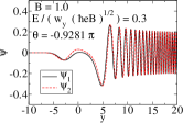
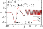
 (c)                                     (d)

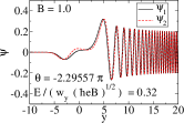
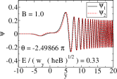
Figure 2: (Color online) Wave functions in the three-quarter Dirac point obtained numerically with $E/(w_{y}\sqrt{\hbar eB})=0.3$ (a), $0.31$ (b), $0.32$ (c), and $0.33$ (d). Parameters are $w_{x}=w_{y}=1$, $w_{0x}=-1$, $w_{0y}=0$, $\alpha_{2}^{\prime}\sqrt{\hbar eB}/w_{y}=\alpha_{2}^{\prime}\sqrt{\hbar eB}/w_{y}=0.01$, and $B=1$. The boundary condition at $y=20$ is taken to be Eq. (33).

(a)                                     (b)

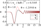
Figure 3: (Color online) Wave functions in the three-quarter Dirac point obtained numerically with $E/(w_{y}\sqrt{\hbar eB})=0.3105$ (a), and $0.3108$ (b).Parameters are $w_{x}=w_{y}=1$, $w_{0x}=-1$, $w_{0y}=0$, $\alpha_{2}^{\prime}\sqrt{\hbar eB}/w_{y}=\alpha_{2}^{\prime\prime}\sqrt{\hbar eB}/w_{y}=0.01$, and $B=1$. The boundary condition at $y=20$ is taken to be Eq. (33).

(a)                                (b)

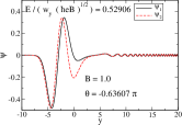
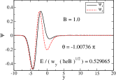
 (c)
    

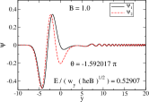
Figure 4: (Color online) Wave functions in the three-quarter Dirac point obtained numerically with $E/(w_{y}\sqrt{\hbar eB})=0.52906$ (a), $0.529065$ (b), and $0.52907$ (c). Parameters are $w_{x}=w_{y}=1$, $w_{0x}=-1$, $w_{0y}=0$, $\alpha_{2}^{\prime}\sqrt{\hbar eB}/w_{y}=\alpha_{2}^{\prime\prime}\sqrt{\hbar eB}/w_{y}=0.01$, and $B=1$. The boundary condition at $y=20$ is taken to be Eq. (33).

We seek the solution of Eq.(24) with $E\geq 0$ which satisfies the conditions that at $y\to-\infty$

$$\Psi_{1}(y)\to 0,$$ (31)

$$\Psi_{2}(y)\to 0.$$ (32)

Note that $y\to-\infty$ corresponds to $q_{x}\to+\infty$, as seen in Eq. (22). When $y\to+\infty$, $\Psi_{1}(y)$ and $\Psi_{2}(y)$ do not have to vanish because the lower band becomes positive when $q_{x}\to-\infty$ at $B=0$ as seen in Fig. 1. Therefore, the conditions, Eqs. (31) and (32) at $y\to-\infty$, do not make the energy quantized. There is the solution for any value of $E$, but the conditions, Eqs. (31) and (32) at $y\to-\infty$, make the restriction for the solutions. We solve the differential equations, Eq. (24), numerically by the fourth-order Runge-Kutta method in this and the next subsections. We take the step size in the Runge-Kutta method to be $0.01$. Since Eq. (24) is the real linear differential equations, the solutions can be taken as real functions, and the solutions multiplied by any constant values give the same solutions. Therefore, for each value of $E$ the only adjustable parameter to obtain the solution numerically by the Runge-Kutta method starting from a fixed $y=y_{+}>0$ and decreasing $y$ is the ratio $\Psi_{2}(y_{+})/\Psi_{1}(y_{+})$. In this subsection we take $y_{+}=20$. It is convenient to parametrize the ratio in terms of the angle $\theta$ defined by

$$\frac{\Psi_{2}(y=20)}{\Psi_{1}(y=20)}=\tan\theta.$$ (33)

The numerically obtained solution diverges as $y$ becomes a negative large value, if the chosen $\theta$ is not a suitable value for the given $E$. Only when $\theta$ is the correct value for $E$, the numerically obtained solution becomes zero as $y\to-\infty$. In this way we determine $\theta$ for any given $E>0$. The boundary condition $\theta$ depends on the choice of $y_{+}$ and it does not have an important meaning. The $E$-dependence of $\theta$, however, is important to obtain the almost-localized state. When $E$ is changed continuously, $\theta$ changes continuously. Note that the energy is semi-classically quantized by the magnetic field, since the closed Fermi surface $\varepsilon_{\textrm{tqD}_{+}}^{0}(\mathbf{q})$ exists at $B=0$. Quantum mechanically, these quantized states in $y\lesssim 0$ couple to the continuous-energy states, which exist mainly in $y\gtrsim 0$, by tunneling. With this mixing of the states $\theta$ changes by $\pi$ in the small region of energy variation. Note that $\theta$ and $\theta+n\pi$ with integer $n$ give the same condition. We show some examples of the solutions for $0.3\leq E/(w_{y}\sqrt{\hbar eB})\leq 0.33$ in Fig. 2 and Fig. 3 and for $0.52906\leq E/(w_{y}\sqrt{\hbar eB})\leq 0.52907$ in Fig. 4, where we have normalized the wave functions numerically as

$$\int_{-10}^{20}\left(|\Psi_{1}(y)|^{2}+|\Psi_{2}(y)|^{2}\right)dy=1.$$ (34)

(a)

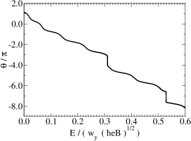
 (b)                                (c)

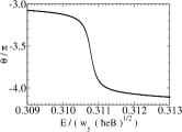
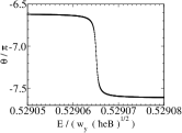
Figure 5: (Color online) Boundary condition $\theta$ at $y=20$ (Eq. (33)) as a function of energy for $w_{x}=w_{y}=1$, $w_{0x}=-1$, $w_{0y}=0$, $\alpha_{2}^{\prime}\sqrt{\hbar eB}/w_{y}=\alpha_{2}^{\prime\prime}\sqrt{\hbar eB}/w_{y}=0.01$, and $B=1$. (b) and (c) are the close-up of (a) near the energy of the almost-localized states at $y\lesssim 0$.

Nearly-localized states in $y\lesssim 0$ exist at $E/(w_{y}\sqrt{\hbar eB})\approx 0.3108$ and $0.529065$. The wave functions $(\Psi_{1}(y),\Psi_{2}(y))$ at $E=0.3105$ and $0.3108$ with the suitable boundary conditions have one node of $\Psi_{1}(y)$ and $\Psi_{2}(y)$ in $y\lesssim 0$, as seen in Fig. 3 (a) and (b), and the wave functions at $E/(w_{y}\sqrt{\hbar eB})=0.52906$, $0.529065$, and $0.52807$ have two nodes in $y\lesssim 0$, as seen in Fig. 4 (a) - (c). Therefore, $E/(w_{y}\sqrt{\hbar eB})\approx 0.3108$ and $E/(w_{y}\sqrt{\hbar eB})\approx 0.529065$ are the nearly-localized state energies with $n=1$ and $n=2$, respectively. Due to the tunneling these nearly-localized states are not completely localized in the region $y\lesssim 0$, which corresponds to the region $q_{x}\gtrsim 0$ in the case of $B=0$ (see Eq. (22) and Fig. 1). This interpretation of the nearly-localized states in three-quarter Dirac point is justified by plotting $\theta$ as a function of energy (Fig. 5). As seen in Fig. 5, $\theta$ changes continuously as $E$ increases. When the energy is close to one of the energies of the nearly-localized states, $\theta$ changes by $\pi$ in a narrow range of $E$. At $n=2$ ($E/(w_{y}\sqrt{\hbar eB})\approx 0.529065$) $\theta$ changes in a narrower range of the energy $E$ than at $n=1$ ($E/(w_{y}\sqrt{\hbar eB})\approx 0.3108$). The narrowing of the range in $\theta$ is reasonable because the tunneling of the almost-localized state at $y\lesssim 0$ into the region of $y\gtrless 0$ is weaker at $n=2$ than at $n=1$.

(a)
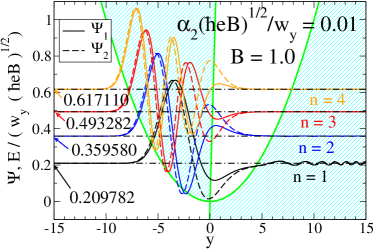
        (b)

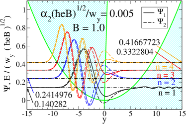
Figure 6: (Color online) Green lines are $\varepsilon_{\mathrm{tqD}_{\pm}}(q_{x},q_{y}=0)/(w_{y}\sqrt{\hbar eB})$ as a function of $y=-q_{x}/(\ell eB)=-q_{x}/\sqrt{\hbar eB}$, i.e. $E/(w_{y}\sqrt{\hbar eB})=(\alpha_{2}\sqrt{\hbar eB}/w_{y})y^{2}$ and $E/(w_{y}\sqrt{\hbar eB})=(2w_{x}/w_{y})y+(\tilde{\alpha}_{2}\sqrt{\hbar eB}/w_{y})y^{2}$. Classical particles can exist in the cyan-shaded regions. Wave functions of almost-localized state with the quantum number $n=1$, $2$, $3$, and $4$ near the three-quarter Dirac point are plotted as functions of $y$. Zero of the wave functions are shifted to their energies. Wave functions are calculated with the boundary conditions at $y=-15$ as in section II C. Parameters are $B=1$, $w_{x}=w_{y}=1$, $w_{0x}=-1$, $w_{0y}=0$ in (a) and (b), and $\alpha_{2}^{\prime}\sqrt{\hbar eB}/w_{y}=\alpha_{2}^{\prime\prime}\sqrt{\hbar eB}/w_{y}=0.005$ ($\alpha_{2}\sqrt{\hbar eB}/w_{y}=0.01$) in (a) and $\alpha_{2}^{\prime}\sqrt{\hbar eB}/w_{y}=\alpha_{2}^{\prime\prime}\sqrt{\hbar eB}/w_{y}=0.0025$ ($\alpha_{2}\sqrt{\hbar eB}/w_{y}=0.005$) in (b).

In Fig. 6, we plot $\varepsilon_{\textrm{tqD}_{\pm}}(q_{x},q_{y}=0)$ at $B=0$ (Eqs. (10) and (14)) with replacing $q_{x}\to-eB\ell y$ (Eq. (22)) divided by the energy scale of the massless Dirac fermions ($w_{y}\sqrt{\hbar eB}$) as a function of dimensionless length $y$ for the dimensionless parameter $\alpha_{2}\sqrt{\hbar eB}/wy=0.01$ (a) and $0.005$ (b). In these figures we also plot the wave functions of the almost-localized states at $y\lesssim 0$ with the quantum number $n=1-4$, which are calculated using the boundary condition at $y=y_{-}<0$ discussed in the next subsection. Classically, electrons can exist in the cyan-shaded regions in Fig. 6, and they can exist only by the quantum tunneling effect in the white regions. For the larger energy (larger quantum number $n$) the width and the hight of the classically-forbidden region (white region in Fig. 6) is larger. As a result the tunneling of the almost localized state with the larger quantum number at $y\lesssim 0$ into the $y\gtrsim 0$ region becomes smaller. Therefore, the numerical solutions of the bound states $n\geq 3$ are difficult to obtain by using the boundary condition at $y=y_{+}>0$, Eq. (33), since $\theta$ changes by $\pi$ in a very narrow region in energy. On the other hand, the almost-localized state with the quantum number $n=1$ couples strongly to the continuous states at $y\gtrsim 0$ as seen in Fig. 5(b), and the energy of the almost-localized state is “broadened”.

In the next subsection we use the boundary condition at $y<0$ to obtain the energy of the bound states.

II.3 numerical results of energy at $B>0$, using boundary condition at $y<0$

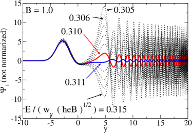
Figure 7: (Color online) Wave function $\Psi_{1}(y)$ in the three-quarter Dirac point obtained numerically by using the boundary condition at $y=-10$. Parameters are $w_{x}=w_{y}=1$, $w_{0x}=-1$, $w_{0y}=0$, $\alpha_{2}^{\prime}\sqrt{\hbar eB}/w_{y}=\alpha_{2}^{\prime\prime}\sqrt{\hbar eB}/w_{y}=0.01$, and $B=1$. We take several values of $E$, and we find that an eigenvalue for the nearly localized state at $y<0$ exists in the region $0.310<E/(w_{y}\sqrt{\hbar eB})<0.311$.

As shown in the previous subsection, it is difficult to obtain the energy of the almost-localized states at $y\lesssim 0$ with a large quantum number $n$ in Eq.(24) by using the boundary condition at $y=y_{+}>0$, since the boundary condition changes in a very narrow region and the energy of the almost-localized states at $y\lesssim 0$ may be overlooked. Therefore, we try to obtain the energy by using the boundary conditions at $y<0$. We study the solutions of Eq.(24) at $y\to-\infty$, assuming

$$\Psi_{j}(y)=c_{j}(y)e^{-g(y)},$$ (35)

($j=1,2$) and

$$\frac{d\Psi_{j}}{dy} =\left(-\frac{dg(y)}{dy}c_{j}(y)+\frac{dc_{j}(y)}{dy}\right)e^{-g(y)}$$

$$\sim-\frac{dg(y)}{dy}c_{j}e^{-g(y)},$$ (36)

as $y\to-\infty$. Then we obtain the equation

$$\begin{pmatrix}(\tilde{\cal{H}}_{\textrm{tqD}})_{11}&(\tilde{\cal{F}}_{\textrm{tqD}})_{12}\\ (\tilde{\cal{F}}_{\textrm{tqD}})_{21}&(\tilde{\cal{H}}_{\textrm{tqD}})_{22}\end{pmatrix}\begin{pmatrix}\Psi_{1}(y)\\ \Psi_{2}(y)\end{pmatrix}\approx E\begin{pmatrix}\Psi_{1}(y)\\ \Psi_{2}(y)\end{pmatrix},$$ (37)

where $(\tilde{\cal{H}}_{\textrm{tqD}})_{11}$ and $(\tilde{\cal{H}}_{\textrm{tqD}})_{22}$ are given in Eqs. (25) and (28) and

$$(\tilde{\cal{F}}_{\textrm{tqD}})_{12} =w_{y}\sqrt{\hbar eB}\left(\frac{dg}{dy}-\frac{w_{x}}{w_{y}}y+\frac{\alpha^{\prime\prime}\sqrt{\hbar eB}}{w_{y}}y^{2}\right),$$ (38)

$$(\tilde{\cal{F}}_{\textrm{tqD}})_{21} =w_{y}\sqrt{\hbar eB}\left(-\frac{dg}{dy}-\frac{w_{x}}{w_{y}}y+\frac{\alpha^{\prime\prime}\sqrt{\hbar eB}}{w_{y}}y^{2}\right).$$ (39)

The nontrivial solution exists when the condition

$$\det\begin{pmatrix}(\tilde{\cal{H}}_{\textrm{tqD}})_{11}-E&(\tilde{\cal{F}}_{\textrm{tqD}})_{12}\\ (\tilde{\cal{F}}_{\textrm{tqD}})_{21}&(\tilde{\cal{H}}_{\textrm{tqD}})_{22}-E\end{pmatrix}=0,$$ (40)

is fulfilled, i.e.,

$$\left(\frac{dg}{dy}\right)^{2} =\left(\frac{\alpha_{2}\sqrt{\hbar eB}}{w_{y}}y^{2}-\frac{E}{w_{y}\sqrt{\hbar eB}}\right)$$

$$\times\left(-\frac{2w_{x}}{w_{y}}y-\frac{\tilde{\alpha}_{2}\sqrt{\hbar eB}}{w_{y}}y^{2}+\frac{E}{w_{y}\sqrt{\hbar eB}}\right),$$ (41)

In the simple case that $\alpha_{2}>0$, $\tilde{\alpha}_{2}=0$ (i.e., $\alpha^{\prime}=\alpha^{\prime\prime}=\alpha_{2}/2$), and large $|y|$, we can neglect terms proportional to $E$. Then the approximate solution is

$$g(y)\sim\pm\frac{2\sqrt{2\alpha_{2}w_{x}\sqrt{\hbar eB}}}{5w_{y}}(-y)^{\frac{5}{2}}+\textrm{const.}$$ (42)

The solution which does not diverge at $y\to-\infty$ is obtained as

$$\begin{pmatrix}\Psi_{1}\\ \Psi_{2}\end{pmatrix}\sim\exp\left(-\frac{2\sqrt{2\alpha_{2}w_{x}\sqrt{\hbar eB}}}{5w_{y}}(-y)^{\frac{5}{2}}\right)\begin{pmatrix}c_{1}\\ c_{2}\end{pmatrix}.$$ (43)

Inserting Eq. (43) into Eq. (37) we obtain the approximate boundary condition at $y\to-\infty$ as

$$\frac{\Psi_{1}(y)}{\Psi_{2}(y)} \sim\frac{c_{1}(y)}{c_{2}(y)}$$

$$\sim\frac{w_{x}+{\alpha_{2}^{\prime}}B\sqrt{\hbar eB}y}{w_{x}-{\alpha_{2}^{\prime\prime}}\sqrt{\hbar eB}y-\sqrt{2\alpha_{2}w_{x}\sqrt{\hbar eB(-y)}}}.$$ (44)

With this boundary conditions at $y=y_{-}=-10.0$ we solve the differential equation Eq. (24) numerically in the Runge-Kutta method with increasing $y$. When we take $E$ to be one of the correct values of the Landau levels, the wave function is nearly localized at $y\lesssim 0$ and tunnels to $y>0$ very little. On the other hand, if we take the different value of $E$, the wave function becomes large as $y$ is increased at $y>0$, although it does not diverge. As shown in Fig. 7, the wave function in the region $y>0$ calculated numerically with the boundary condition at $y_{-}=-10$ becomes small only when we take the correct eigenvalue $0.310<E<0.311$. This value is consistent with the $n=1$ eigenvalue obtained numerically with the boundary condition at $y_{+}=20$ (Fig. 3). We also check numerically that the solution is not sensitive to the boundary condition; numerically the same result is obtained even when we take $\Psi_{1}=0$ and $\Psi_{2}\neq 0$ at $y=y_{-}=-10$. The independence on the boundary condition can be understood as follows. As seen in section II B, the coupling between the nearly-localized state at $y\lesssim 0$ and the continuous state as $y\gtrsim 0$ is small for $n\geq 2$. In section II B we first fixed the energy and obtain the wave functions not divergent at $y\to-\infty$ by changing the boundary condition at $y_{+}>0$ ($\theta$ at $y_{+}=20$). In this section we first take the approximate boundary condition at $y_{-}=-10$, and obtain the energy which gives the smallest amplitude of oscillations of the wave function at $y>0$. Even though the boundary condition is not exact, suitable linear combination of the nearly-localized state at $y\lesssim 0$ and continuous state as $y\gtrsim 0$ may give the non-divergent solution with the given boundary condition at $y=y_{-}$, if the energy is the correct energy of the nearly-localized state at $y\lesssim 0$.

In Fig. 8 we show the wave functions for nearly-localized states with quantum numbers $n=0$ – $6$.

(a)                                (b)

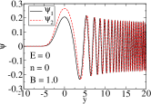
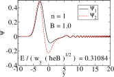
 (c)                                (d)

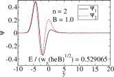
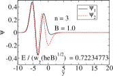
 (e)                                (f)

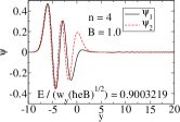
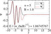
 (g)
    

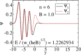
Figure 8: (Color online) Wave functions of nearly localized eigenstates at $y<0$ with quantum number (a) $n=0$, (b) $n=1$, (c) $n=2$, (d) $n=3$, (e) $n=4$, (f) $n=5$, and (g) $n=6$ in the three-quarter Dirac point obtained numerically with the boundary condition at $y=-10$. Parameters are $w_{x}=w_{y}=1$, $w_{0x}=-1$, $w_{0y}=0$, $\alpha_{2}^{\prime}\sqrt{\hbar eB}/w_{y}=\alpha_{2}^{\prime\prime}\sqrt{\hbar eB}/w_{y}=0.01$, and $B=1$.

For $n=0$, i.e. $E=0$, both components of the wave function have a broad peak at $y=0$, although each component of the wave functions is not small at $y>0$, as shown in Fig. 8(a). The oscillation of the wave function at $y>0$ can be understood as the continuous energy states at $y>0$. Since the upper band touches the lower band at the three-quarter Dirac point without the boundary barrier, the nearly-localized state at $y<0$ goes through to the region $y>0$. We will discuss the $n=0$ state in the next section.

The eigenstate for $n\geq 1$ is obtained by taking the suitable value of $E$, which minimize the amplitude of oscillation of the wave function in the region $y>0$. We find the tunneling through the barrier is smaller as $n$ becomes larger, as we have discussed in the previous subsection.

We also calculate the energy as a function of quantum number $n$ with different choice of parameters $\alpha_{2}^{\prime}\sqrt{\hbar eB}/w_{y}=0.02$ and $\alpha_{2}^{\prime\prime}=0$ from these used in Fig. 8 ($\alpha_{2}^{\prime}\sqrt{\hbar eB}/w_{y}=\alpha_{2}^{\prime\prime}\sqrt{\hbar eB}/w_{y}=0.01$). We plot the energy as a function of $n$ in Fig. 9. We obtain

$$E_{n}\propto n^{\frac{4}{5}}.$$ (45)

In Figs. 10 and 11 we plot the energy as a function of $\alpha_{2}$ and $B$, respectively. We obtain

$$E_{n}\propto\alpha_{2}^{\frac{3}{5}}(nB)^{\frac{4}{5}}.$$ (46)

We have previously obtained $n$ and $B$ dependence at the three-quarter Dirac point (Eq. (46)) in the tight-binding model of $\alpha$-(BEDT-TTF)₂I₃ at the critical pressureKishigi and Hasegawa (2017).

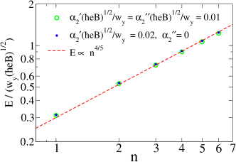
Figure 9: (Color online) Energy as a function of the quantum number $n$ for the three-quarter Dirac point. Parameters are $w_{x}=w_{y}=1$, $w_{0x}=-1$, $w_{0y}=0$, and $B=1$. We take two choices of parameters giving the same $\alpha_{2}$, $\alpha_{2}^{\prime}\sqrt{\hbar eB}/w_{y}=\alpha_{2}^{\prime\prime}\sqrt{\hbar eB}/w_{y}=0.01$ and $\alpha_{2}^{\prime}\sqrt{\hbar eB}/w_{y}=0.02$, $\alpha_{2}^{\prime\prime}=0$. The obtained values of the energy is well fitted by the red broken line ($E\propto 0.3n^{\frac{4}{5}}$).

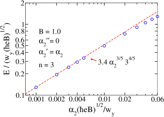
Figure 10: (Color online) Energy with the quantum number $n=3$ as a function of $\alpha_{2}$ for the three-quarter Dirac point. Parameters are $w_{x}=w_{y}=1$, $w_{0x}=-1$, $w_{0y}=0$, $\alpha_{2}^{\prime\prime}=0$, and $B=1$.

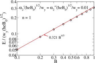
Figure 11: (Color online) Dimensionless energy ($E/(w_{y}\sqrt{\hbar eB_{0}})$ with $B_{0}=1$) as a function of magnetic field $B$ at the three quarter Dirac point. It is well fitted as a function of $B^{\frac{4}{5}}$.

II.4 analytical study with approximation in the magnetic-field- and $\alpha_{2}$-dependence of the Landau levels at the three-quarter Dirac point

In this subsection we give the analytical derivation of Eq. (46). Taking a sum and a difference, we obtain the equations

$$\left[\frac{\alpha_{2}\sqrt{\hbar eB}}{w_{y}}{y}^{2}-\frac{E}{w_{y}\sqrt{\hbar eB}}\right]\left(\Psi_{1}+\Psi_{2}\right)$$

$$+\frac{d}{d{y}}\left(\Psi_{1}-\Psi_{2}\right)=0,$$ (47)

$$\left[\frac{2w_{x}}{w_{y}}y+\frac{\tilde{\alpha}_{2}\sqrt{\hbar eB}}{w_{y}}{y}^{2}-\frac{E}{w_{y}\sqrt{\hbar eB}}\right]\left(\Psi_{1}-\Psi_{2}\right)$$

$$-\frac{d}{d{y}}\left(\Psi_{1}+\Psi_{2}\right)=0.$$ (48)

In the three-quarter Dirac case studied in this paper the term proportional to ${y}$ in Eq. (47) does not exist and the term proportional to ${y}^{2}$ in Eq. (47) cannot be neglected, while the term proportional to ${y}^{2}$ in Eq. (48) can be neglected. Then there appear dimensionless parameters $\alpha_{2}\sqrt{\hbar eB}/w_{y}$ and $w_{x}/w_{y}$. The energy depends not only the energy scale $w_{y}\sqrt{\hbar eB}$ but also these dimensionless parameters. Therefore, we may expect

$$E\propto\left(w_{y}\sqrt{\hbar eB}\right)\left(\frac{\alpha_{2}\sqrt{\hbar eB}}{w_{y}}\right)^{\beta}\left(\frac{w_{x}}{w_{y}}\right)^{\eta}n^{\delta},$$ (49)

where $n$ is the quantum number of the almost localized state at $y\lesssim 0$. We determine the exponents, $\beta$, $\eta$ and $\delta$. We take

$$\beta>0,$$ (50)

in order to obtain $E\to 0$ as $\alpha_{2}\to 0$. The almost-localized state has the finite absolute value of $|\Psi_{1}+\Psi_{2}|$ in the region

$$-{y}_{0}\lesssim{y}\lesssim 0,$$ (51)

and it is exponentially small in the region

$${y}\lesssim-{y}_{0},$$ (52)

where the dimensionless length ${y}_{0}$ is determined by the equation

$$\frac{\alpha_{2}\sqrt{\hbar eB}}{w_{y}}y_{0}^{2}=\frac{E}{w_{y}\sqrt{\hbar eB}}\sim\left(\frac{\alpha_{2}\sqrt{\hbar eB}}{w_{y}}\right)^{\beta}\left(\frac{w_{x}}{w_{y}}\right)^{\eta}n^{\delta}.$$ (53)

Then $y_{0}$ depends on the dimensionless parameters as

$$y_{0}\sim\left(\frac{\alpha_{2}\sqrt{\hbar eB}}{w_{y}}\right)^{\frac{\beta-1}{2}}\left(\frac{w_{x}}{w_{y}}\right)^{\frac{\eta}{2}}n^{\frac{1}{2}\delta}.$$ (54)

We expect

$$\left\langle\left|\frac{d}{dy}(\Psi_{1}-\Psi_{2})\right|\right\rangle\sim\frac{2cn}{{y}_{0}}\Bigl{\langle}\sqrt{|\Psi_{1}-\Psi_{2}|^{2}}\Bigr{\rangle},$$ (55)

where $\langle\cdots\rangle$ is the spacial average in ${y}_{0}\lesssim{y}\lesssim 0$ and $c$ is a dimensionless constant of order $1$. This approximation is not justified for small $n$. However, we may consider that $(\Psi_{1}-\Psi_{2})$ changes sign $n$ times in the length of $y_{0}$, i.e., $(\Psi_{1}-\Psi_{2})$ changes from $\pm c\left\langle\sqrt{|\Psi_{1}-\Psi_{2}|^{2}}\right\rangle$ to $\mp c\left\langle\sqrt{|\Psi_{1}-\Psi_{2}|^{2}}\right\rangle$ periodically in the half period ($y_{0}/n$). Approximating the oscillation of $(\Psi_{1}-\Psi_{2})$ by a triangle wave, we obtain Eq. (55). This crude approximation will give an approximate dependence on $n$ and $y_{0}$ in Eq. (55) in the limit of $n\gg 1$. With this approximation we obtain

$$\frac{\Bigl{\langle}\sqrt{|\Psi_{1}-\Psi_{2}|^{2}}\Bigr{\rangle}}{\Bigl{\langle}\sqrt{|\Psi_{1}+\Psi_{2}|^{2}}\Bigr{\rangle}}\sim\left(\frac{\alpha_{2}\sqrt{\hbar eB}}{w_{y}}\right)^{\frac{3\beta-1}{2}}\left(\frac{w_{x}}{w_{y}}\right)^{\frac{3}{2}\eta}(2cn)^{\frac{3\delta-2}{2}},$$ (56)

by taking the spacial average in Eq. (47). Next, we examine Eq. (48) in the same way. The second term and the third term in the coefficient of $\Psi_{1}-\Psi_{2}$ in Eq. (48), which depend on the dimensionless parameter as $\left(\alpha_{2}\sqrt{\hbar eB}/w_{y}\right)^{\beta}$, can be neglected with respect to the first term in the coefficient of $\Psi_{1}-\Psi_{2}$, since we study the case

$$\frac{\alpha_{2}\sqrt{\hbar eB}}{w_{y}}\ll\frac{w_{x}}{w_{y}}.$$ (57)

Then we obtain

$$\frac{\Bigl{\langle}\sqrt{|\Psi_{1}-\Psi_{2}|^{2}}\Bigr{\rangle}}{\Bigl{\langle}\sqrt{|\Psi_{1}+\Psi_{2}|^{2}}\Bigr{\rangle}}\sim\left(\frac{\alpha_{2}\sqrt{\hbar eB}}{w_{y}}\right)^{1-\beta}\left(\frac{w_{x}}{w_{y}}\right)^{1-\eta}(2cn)^{-\delta-1}.$$ (58)

Comparing Eq. (56) and Eq. (58), we obtain

$$\beta=\frac{3}{5},$$ (59)

$$\eta=-\frac{2}{5},$$ (60)

and

$$\delta=\frac{4}{5}.$$ (61)

Inserting these exponents in Eq. (49), we obtain

$$E\sim w_{x}^{-\frac{2}{5}}w_{y}^{\frac{4}{5}}\alpha_{2}^{\frac{3}{5}}(n\hbar eB)^{\frac{4}{5}}.$$ (62)

In Appendix we give a simpler derivation of Eq. (62).

This result is consistent with the result obtained by the semiclassical quantization rule in the previous paperKishigi and Hasegawa (2017), in which the energy is quantized as

$$A(E_{n})\propto(n+\gamma)B,$$ (63)

where $\gamma$ is a phase factor ($\gamma=1/2$ for 2D free electrons and semi-Dirac fermions and $\gamma=0$ for Dirac fermions and three-quarter Dirac fermions) and $A(\varepsilon)$ is the area of the Fermi surface in the 2D $\mathbf{k}$-space at $B=0$ with the Fermi energy $\varepsilon$. The area, $A(\epsilon)$, and the density of states, $D(\epsilon)$, are related by

$$\frac{1}{4\pi^{2}}\frac{dA(\varepsilon)}{d\varepsilon}=D(\varepsilon).$$ (64)

We plot $A(\varepsilon)$ and $D(\varepsilon)$ in Fig. 12. In the three-quarter Dirac case, we have obtainedKishigi and Hasegawa (2017)

$$A(\varepsilon)\propto\alpha_{2}^{-\frac{3}{4}}\varepsilon^{\frac{5}{4}},$$ (65)

in the limit $\epsilon\to 0$, and

$$E_{n}\propto\alpha_{2}^{\frac{3}{5}}(nB)^{\frac{4}{5}}.$$ (66)

(a)                                     (b)

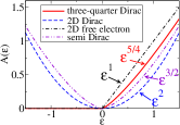
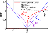
Figure 12: (Color online) Schematic plot of the areas of the Fermi surface and the density of states as a function of energy for the three-quarter Dirac fermion, massless 2D Dirac fermion, 2D free fermion, and 2D semi Dirac fermionHasegawa et al. (2006); Dietl et al. (2008). The density of states are scaled to be 1 at $\epsilon=1$.

III finite energy gap and $n=0$ state

In this section we study the $n=0$ state by introducing the energy gap in the three-quarter Dirac point, which may be caused by a difference of the site energy in two sublattices,

$$\mathcal{H}_{\textrm{tqD}}^{\prime}=\mathcal{H}_{\textrm{tqD}}+\begin{pmatrix}\Delta&0\\ 0&-\Delta\end{pmatrix},$$ (67)

where $2|\Delta|$ is the energy gap at the three-quarter Dirac point. Note that the minimum of the upper band is not at the three-quarter Dirac point ($\mathbf{q}=0$) and the minimum energy of the upper band is not $|\Delta|$. Then the equation we study at $B\neq 0$ is

$$\begin{pmatrix}(\tilde{\cal{H}}_{\textrm{tqD}})_{11}+\Delta&(\tilde{\cal{H}}_{\textrm{tqD}})_{12}\\ (\tilde{\cal{H}}_{\textrm{tqD}})_{21}&(\tilde{\cal{H}}_{\textrm{tqD}})_{22}-\Delta\end{pmatrix}\begin{pmatrix}\Psi_{1}(y)\\ \Psi_{2}(y)\end{pmatrix}= E\begin{pmatrix}\Psi_{1}(y)\\ \Psi_{2}(y)\end{pmatrix}.$$ (68)

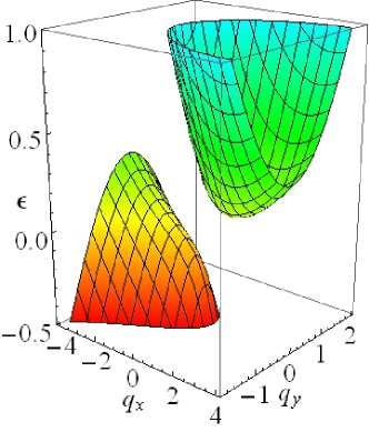
Figure 13: (Color online) Energy at $B=0$ as a function of $q_{x}$ and $q_{y}$ with parameters $w_{x}=0.4$, $w_{y}=1$, $\alpha_{2}^{\prime}=\alpha_{2}^{\prime\prime}=0.01$, $w_{0x}=-w_{x}$, $w_{0y}=0$, and $\Delta=\pm 0.3$.

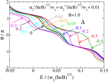
Figure 14: (Color online) Boundary condition $\theta$ at $y=y_{+}=20$ (Eq. (33)), which makes $|\Psi_{1,2}(y)|\to 0$ at $y\to-\infty$, as a function of the energy. We take parameters $w_{x}=w_{y}=1$, $\alpha_{2}^{\prime}\sqrt{\hbar eB}/w_{y}=\alpha_{2}^{\prime\prime}\sqrt{\hbar eB}/w_{y}=0.01$, $\Delta=0.3$, $0.2$, $\cdots$, $-0.3$, $-0.4$, and $B=1$.

(a)                                (b)

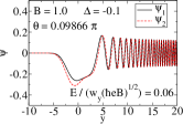
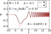
 (c)                                (d)

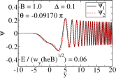
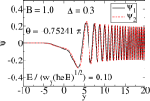
Figure 15: (Color online) Wave functions for (a) $\Delta=-0.1$, $E/(w_{y}\sqrt{\hbar eB})=0.06$, (b) $\Delta=-0.3$, $E/(w_{y}\sqrt{\hbar eB})=0.10$, (c) $\Delta=0.1$, $E/(w_{y}\sqrt{\hbar eB})=0.06$, and (d) $\Delta=0.3$, $E/(w_{y}\sqrt{\hbar eB})=0.10$, Other parameters are $w_{x}=w_{y}=1$, $\alpha_{2}^{\prime}\sqrt{\hbar eB}/w_{y}=\alpha_{2}^{\prime\prime}\sqrt{\hbar eB}/w_{y}=0.01$, and $B=1$. Boundary conditions at $y=20$ ($\theta$) are taken as in the case of $\Delta=0$ in section II B. The wave functions have large amplitudes in $y\lesssim 0$ region, when $\Delta<0$ [(a) and (b)], while no peaks are seen in $y\lesssim 0$ region, when $\Delta>0$ [(c) and (d)].

Although the energy dispersion at $B=0$ does not depend on the sign of $\Delta$, the quantized energies at $B\neq 0$ are not the same for $\pm\Delta\neq 0$. We take $\alpha_{2}^{\prime}=\alpha_{2}^{\prime\prime}=0.01$ and $B=1$ and we calculate the wave functions numerically with the boundary condition at $y=20$, as in Section II.2. We plot the boundary condition $\theta$ to exist a non-divergent solution as a function of energy in Fig. 14. For $\Delta\lesssim-0.1$, $\theta$ changes in a narrow region of $E$, which indicate that an almost-localized state exists at $y\lesssim 0$ as shown in Fig. 15 (a) and (b), while the variation of $\theta$ as a function of $E$ becomes broad for $\Delta\geq-0.1$, which indicate that an almost-localized state at $y\lesssim 0$ couples strongly to the continuous energy state at $y>0$ and an almost-localized state ceases to exist at $y\lesssim 0$ as shown in Fig. 15 (c) and (d). We think that the eigenstate with $n=0$ does not exist when $\Delta>0$, but the almost-localized state exists at $y\lesssim 0$ when $\Delta\leq 0$. The effect of the tunneling would become important as $\Delta$ approaches to zero and the almost-localized $n=0$ state at $y\lesssim 0$ couples strongly to the continuous energy levels in $y>0$. This situation that the $n=0$ mode exists only when $\Delta\leq 0$ is similar to the model studied by HaldaneHaldane (1988), where the zero mode exists either upper band or lower band depending on the sign of the mass, which is $\Delta$ in the present model, and the direction of the magnetic field. In our model the nearly bound state with $n=0$ exists when $\Delta\leq 0$. The $n=0$ ($E=0$) state at $\Delta=0$ in Fig. 8(a) is understood as the zero-mode of the almost-localized state at three-quarter Dirac point, which couples strongly to the continuous states at $y\gtrsim 0$. Note that the simultaneous changes of $B\leftrightarrow-B$, $y\leftrightarrow-y$, $\Psi_{1}\leftrightarrow\Psi_{2}$, and $\Delta\leftrightarrow-\Delta$ do not change Eq. (68).

IV Summary

We study the quantized energy at the three-quarter Dirac point in the presence of external magnetic field $B$. We obtain that the quantized energy is proportional to $\alpha_{2}^{\frac{3}{5}}(nB)^{\frac{4}{5}}$ (Eq. (46)) by calculating the solution of the differential equation (Eq. (24)) numerically. We also obtain the approximate result in the limit of $|\alpha_{2}\sqrt{\hbar eB}/w_{y}|\ll 1$ as $E\propto w_{x}^{-\frac{2}{5}}w_{y}^{\frac{4}{5}}\alpha_{2}^{\frac{3}{5}}(n\hbar eB)^{\frac{4}{5}}$ (Eq. (62)), which is consistent with the result obtained in the previous paperKishigi and Hasegawa (2017) by using the semiclassical quantization rule. We show that the zero mode exists by studying the finite-gap system. Since the three-quarter Dirac points with the finite gap appear as a pair when the time-reversal symmetry is not broken at $B=0$, sign of $\Delta$ is positive at one finite-gap three-quarter Dirac point and negative at another point. As a result, there is one zero mode in the system when $B\neq 0$ and $\Delta\neq 0$.

The quantization of the energy in the three-quarter Dirac point in a magnetic field can be observed experimentally in quasi-two-dimensional organic superconductor $\alpha$-(BEDT-TTF)₂I₃Kishigi and Hasegawa (2017) and ultra cold Fermi gas on a tunable optical latticeTarruell et al. (2012).

*

Appendix A another derivation of $E\propto\alpha_{2}^{\frac{3}{5}}B^{\frac{4}{5}}$

From Eq. (24) we formally obtain the equation

$$\det\begin{pmatrix}M&N_{-}\\ N_{+}&M\end{pmatrix}=0,$$ (69)

where

$$M =\frac{w_{x}}{w_{y}}y+\frac{\alpha_{2}^{\prime}\sqrt{\hbar eB}}{w_{y}}y^{2}-\frac{E}{w_{y}\sqrt{\hbar eB}},$$ (70)

$$N_{\pm} =\pm\frac{d}{dy}-\frac{w_{x}}{w_{y}}y+\frac{\alpha_{2}^{\prime\prime}\sqrt{\hbar eB}}{w_{y}}y^{2}$$ (71)

to get

$$\frac{E}{w_{y}\sqrt{\hbar eB}} =\frac{w_{x}}{w_{y}}y+\frac{\alpha_{2}^{\prime}\sqrt{\hbar eB}}{w_{y}}y^{2}$$

$$\pm\sqrt{\left(\frac{-w_{x}}{w_{y}}y+\frac{\alpha_{2}^{\prime\prime}\sqrt{\hbar eB}}{w_{y}}y^{2}\right)^{2}-\frac{d^{2}}{dy^{2}}}$$ (72)

The almost localized state in $y<0$ is obtained by taking the expansion

$$\left|\frac{d^{2}}{dy^{2}}\right| \ll\left(\frac{-w_{x}}{w_{y}}y+\frac{\alpha_{2}^{\prime\prime}\sqrt{\hbar eB}}{w_{y}}y^{2}\right)^{2}.$$ (73)

Then we obtain

$$\frac{E}{w_{y}\sqrt{\hbar eB}}\sim\frac{\alpha_{2}\sqrt{\hbar eB}}{w_{y}}y^{2}-\frac{w_{y}}{2w_{x}}\frac{1}{(-y)}\frac{d^{2}}{dy^{2}},$$ (74)

where we have used

$$\left|\frac{\alpha_{2}^{\prime\prime}\sqrt{\hbar eB}}{w_{y}}y^{2}\right|\ll\left|\frac{w_{x}}{w_{y}}y\right|.$$ (75)

Taking a new variable $Y$ as

$$y=\left(\frac{\alpha_{2}\sqrt{\hbar eB}}{w_{y}}\right)^{\sigma}\left(\frac{w_{x}}{w_{y}}\right)^{\nu}Y,$$ (76)

and making the two terms in the right hand side of Eq. (74) to be the same order in the dimensionless parameters $\alpha\sqrt{\hbar eB}/w_{y}$ and $w_{x}/w_{y}$, we obtain

$$\sigma=-\frac{1}{5},$$ (77)

and

$$\nu=-\frac{1}{5}.$$ (78)

Then we obtain

$$E \sim w_{y}\sqrt{\hbar eB}\left(\frac{\alpha_{2}\sqrt{\hbar eB}}{w_{y}}\right)^{\frac{3}{5}}\left(\frac{w_{x}}{w_{y}}\right)^{-\frac{2}{5}}$$

$$\times\left(Y^{2}-\frac{1}{(-2Y)}\frac{d^{2}}{dY^{2}}\right).$$ (79)

Since $Y$ does not depend on any parameters, we obtain

$$E\sim w_{x}^{-\frac{2}{5}}w_{y}^{\frac{4}{5}}\alpha_{2}^{\frac{3}{5}}(\hbar eB)^{\frac{4}{5}}.$$ (80)

References

- Novoselov et al. (2005) A. K. Novoselov, K. S.and Geim, S. V. Morozov, D. Jiang, M. I. Katsnelson, I. V. Grigorieva, S. V. Dubonos, and A. A. Firsov, Nature 438, 197 (2005).
- Zhang et al. (2005) Y. Zhang, Y.-W. Tan, H. L. Stormer, and P. Kim, Nature 438, 201 (2005).
- Tajima et al. (2000) N. Tajima, M. Tamura, Y. Nishio, K. Kajita, and Y. Iye, J. Phys. Soc. Jpn. 69, 543 (2000).
- Katayama et al. (2006) S. Katayama, A. Kobayashi, and Y. Suzumura, J. Phys. Soc. Jpn. 75, 054705 (2006).
- Kajita et al. (2014) K. Kajita, Y. Nishio, N. Tajima, Y. Suzumura, and A. Kobayashi, J. Phys. Soc. Jpn. 83, 072002 (2014).
- Fu et al. (2007) L. Fu, C. L. Kane, and E. J. Mele, Phys. Rev. Lett. 98, 106803 (2007).
- Hsieh et al. (2009) D. Hsieh, Y. Xia, D. Qian, L. Wray, J. H. Dil, F. Meier, J. Osterwalder, L. Patthey, J. G. Checkelsky, N. P. Ong, A. V. Fedorov, H. Lin, A. Bansil, D. Grauer, Y. S. Hor, R. J. Cava, and M. Z. Hasan, Nature 460, 1101 (2009).
- Kobayashi et al. (2007) A. Kobayashi, S. Katayama, Y. Suzumura, and H. Fukuyama, J. Phys. Soc. Jpn. 76, 034711 (2007).
- Goerbig et al. (2008) M. O. Goerbig, J.-N. Fuchs, G. Montambaux, and F. Piéchon, Phys. Rev. B 78, 045415 (2008).
- Kobayashi et al. (2009) A. Kobayashi, Y. Suzumura, H. Fukuyama, and M. O. Goerbig, Journal of the Physical Society of Japan 78, 114711 (2009).
- Kishigi and Hasegawa (2017) K. Kishigi and Y. Hasegawa, Phys. Rev. B 96, 085430 (2017).
- Hasegawa et al. (2006) Y. Hasegawa, R. Konno, H. Nakano, and M. Kohmoto, Phys. Rev. B 74, 033413 (2006).
- Dietl et al. (2008) P. Dietl, F. Piéchon, and G. Montambaux, Phys. Rev. Lett. 100, 236405 (2008).
- Montambaux et al. (2009) G. Montambaux, F. Piéchon, J.-N. Fuchs, and M. O. Goerbig, Eur. Phys. J. B 72, 509 (2009).
- Banerjee et al. (2009) S. Banerjee, R. R. P. Singh, V. Pardo, and W. E. Pickett, Phys. Rev. Lett. 103, 016402 (2009).
- Delplace and Montambaux (2010) P. Delplace and G. Montambaux, Phys. Rev. B 82, 035438 (2010).
- Haldane (1988) F. D. M. Haldane, Phys. Rev. Lett. 61, 2015 (1988).
- Tarruell et al. (2012) L. Tarruell, D. Greif, T. Uehlinger, G. Jotzu, and T. Esslinger, Nature 438, 302 (2012).