Learning Embeddings of Directed Networks with Text-Associated Nodes—with Application in Software Package Dependency Networks

Abstract

A network embedding consists of a vector representation for each node in the network. Its usefulness has been shown in many real-world application domains, such as social networks and web networks. Directed networks with text associated with each node, such as software package dependency networks, are commonplace. However, to the best of our knowledge, their embeddings have hitherto not been specifically studied. In this paper, we propose PCTADW-1 and PCTADW-2, two algorithms based on neural networks that learn embeddings of directed networks with text associated with each node. We create two new node-labeled such networks: The package dependency networks in two popular GNU/Linux distributions, Debian and Fedora. We experimentally demonstrate that the embeddings produced by our algorithms resulted in node classification with better quality than those of various baselines on these two networks. We observe that there exist systematic presence of analogies (similar to those in word embeddings) in the network embeddings of software package dependency networks. To the best of our knowledge, this is the first time that such systematic presence of analogies is observed in network and document embeddings. We further demonstrate that these network embeddings can be novelly used for better understanding software attributes, such as the development process and user interface of software, etc.

I Introduction

Machine learning has a long history of being applied to networks for multifarious tasks, such as network classification [1], prediction of protein binding [2], etc. Thanks to the advancement of technologies such as the Internet and database management systems, the amount of data that are available for machine learning algorithms have been growing tremendously over the past decade. Among these datasets, a huge fraction can be modeled as networks, such as web networks, brain networks, citation networks, street networks, etc. [3]. Therefore, improving machine learning algorithms on networks has become even more important.

However, due to the discrete and sparse nature of networks, it is often difficult to apply machine learning directly to them. To resolve this issue, one major school of thought to approach networks using machine learning is via network embeddings [4]. A network embedding consists of a real number-valued Euclidean vector representation for each node in the network. These vectors can then be fed into machine learning algorithms for various classification and regression tasks.

In recent years, there have been dramatic advancements in learning network embeddings, such as DeepWalk [5] (and its variants using personalized graph or node context distributions [6, 7]), LINE [8], node2vec [9], DNGR [10], metapath2vec [11], M-NMF [12], PRUNE [13], GraphSAGE [14], LANE [15], RSDNE [16], ANE [17], ATP [18] and SIDE [19]. Most of these works, however, focus on the structure of the networks alone and do not take data associated with nodes into account. But, in reality, there exist a huge amount of networks in which each node is associated with text data (a document), such as citation networks with titles and abstracts of articles, web networks with contents of web pages, etc.

To ameliorate this issue, [20] proposed text-associated DeepWalk (TADW), a network embedding learning algorithm that leverages the network and documents associated with nodes. Despite the presence of “DeepWalk” in its name, it does not directly use random walks. Instead, it is based on matrix factorization of adjacency matrices and thus bears scalability issues: Its space requirement scales quadratically with respect to the number of nodes. Therefore, developing an effective and scalable network embedding learning algorithm for networks with text-associated nodes remains imperative. Another related work is Paper2vec [21], which, however, is tailored for research paper citation networks.

One important kind of network with text-associated nodes is software package dependency networks (SPDN). They play essential roles in modern software package management systems. For example, in most cases, when a user installs a software package on a modern GNU/Linux distribution via its software package management system (which is the most common way to install software), an SPDN is queried so that the software package management system installs necessary dependencies of that software package. Unfortunately, to the best of our knowledge, SPDNs have not hitherto been studied in the context of network embeddings (despite that they have been studied in the context of data mining for other purposes, e.g., [22, 23])—the huge literature of network embeddings have been largely focusing on social networks, citation networks, and web networks (e.g., [20, 4]).

In this paper: (1) We create two new directed networks with text-associated and multi-labeled nodes, the package dependency networks in Debian and Fedora, two popular GNU/Linux distributions. (2) We propose parent-child text-associated DeepWalk-1/-2 (PCTADW-1/PCTADW-2), two algorithms for learning network embeddings for directed networks with text-associated nodes, and we demonstrate that PCTADW-1 and PCTADW-2 outperformed other algorithms in terms of effectiveness. (3) The systematic presence of analogies has been long observed in word embeddings and has played an essential role in human understanding of word embeddings and algorithmically understanding words (e.g., [24]). Unfortunately, such analogies have not been systematically observed in network and document embeddings. For the first time, we observe the systematic presence of analogies in network embeddings. (4) We finally demonstrate that a network embedding can be novelly used for better understanding software attributes (SAs), such as how software are developed, software user interface, etc.

II Background

II-A Software Package Dependency Network

A software package dependency network (SPDN) characterizes the dependency relationship between software packages in a software package management system. Simply speaking, a package $A$ depends on a package $B$ iff installing $A$ requires installing $B$ first. They are usually directed networks in which each node represents a software package and each directed edge characterizes a dependency relation. For example, in a SPDN that describes Python packages (such as those in PyPI), there would be an edge that connects the node representing “tensorflow” to the node representing “numpy” to represent the fact that the software package “tensorflow” depends on “numpy.” In addition, in modern software package management systems, each package is usually associated with text description.

II-B Learning Network Embeddings on Networks with Text-Associated Nodes

As mentioned in the introduction, the majority of current network embedding learning algorithms focus on the networks alone without taking into account data associated with nodes, especially text data. TADW is a recently developed algorithm that learns network embeddings on networks with text-associated nodes. It learns a network embedding by factorizing the matrix

$$M=(A+A^{2})/2,$$

where $A$ is the $|V|\times|V|$ probabilistic transition matrix characterizing the transitions of states of a randomly walking agent on the network, i.e.,

$$(A)_{uv}=\begin{cases}1/\deg(u)&\quad\text{if }(u,v)\in E\\ 0&\quad\text{otherwise},\end{cases}$$ (1)

where $\deg(u)$ is the degree of $u$. To incorporate text associated with nodes, TADW multiplies an additional matrix that represents text features during the matrix factorization. In other words, it computes

$$\min_{W,H}||M-W^{\top}HT||^{2}_{F}+\frac{\lambda}{2}\left(||W||^{2}_{F}+||H||^{2}_{F}\right).$$ (2)

Here, $T$ is a matrix consisting of the text feature vector of each node, and $W$ and $H$ are the to-be-learned matrices that consist of vector representations of each node. From the equation above, it is easy to see that the space complexity of TADW scales quadratically with respect to the number of nodes even if the network is sparse and therefore bears a scalability issue.

III Embeddings of Directed Networks

For a given directed network $G=\langle V,E\rangle$, we represent each $v\in V$ using two real number-valued vectors $\boldsymbol{v}_{c}$ and $\boldsymbol{v}_{p}$. $\boldsymbol{v}_{c}$ and $\boldsymbol{v}_{p}$ encode $v$ from two different perspectives—$v$ as a child (from its incoming edges) and parent (from its outgoing edges)—and are referred to as the child vector representation and parent vector representation of $v$, respectively. ($u$ is a parent (node) of $v$ and $v$ is a child (node) of $u$ iff $(u,v)\in E$.) We modify the Skip-gram model [5] as to minimize a negative log probability, i.e., as to compute

$$\begin{split}\operatorname*{arg\,min}_{\begin{subarray}{c}\boldsymbol{v}_{c},\boldsymbol{v}_{c}^{\dagger},\boldsymbol{v}_{p},\boldsymbol{v}_{p}^{\dagger}:v\in V\\ \boldsymbol{u}_{c},\boldsymbol{u}_{c}^{\dagger},\boldsymbol{u}_{p},\boldsymbol{u}_{p}^{\dagger}:u\in V\end{subarray}}L_{g}(G)=-\sum_{\begin{subarray}{c}u,v\in V:\\ u\neq v\end{subarray}}[&w^{c}_{u,v}\log p_{c}(v~{}|~{}u)+\\ &w^{p}_{v,u}\log p_{p}(u~{}|~{}v)],\end{split}$$ (3)

where $w^{c}_{u,v}$ and $w^{p}_{v,u}$ are two non-negative weighting hyperparameters and have cutoffs (i.e., $w^{c}_{u,v}=0$ and $w^{p}_{v,u}=0$ if $\operatorname*{dist}(u,v)>s$, where $s$ is another positive hyperparameter and $\operatorname*{dist}(u,v)$ is the distance from $u$ to $v$ in the directed network), and

$$p_{c}(v~{}|~{}u) =\frac{\exp\left(\boldsymbol{v}^{\dagger\top}_{c}\boldsymbol{u}_{p}\right)}{\sum_{v^{\prime}\in V}\exp\left(\boldsymbol{v}^{\prime\dagger\top}_{c}\boldsymbol{u}_{p}\right)}$$ (4)

$$p_{p}(u~{}|~{}v) =\frac{\exp\left(\boldsymbol{u}_{p}^{\dagger\top}\boldsymbol{v}_{c}\right)}{\sum_{u^{\prime}\in V}\exp\left(\boldsymbol{u}^{\prime\dagger\top}_{p}\boldsymbol{v}_{c}\right)}.$$ (5)

Here, vectors with and without superscript $\dagger$ are analogous to “output” and “input” vectors in [24, Equation (2)], respectively. Equations 4 and 5 have similar forms to [5, Equation (4)] and [24, Equation (2)]. Unlike [5, Equation (4)] and [24, Equation (2)], which train vectors to accurately predict surrounding nodes from given nodes without incorporating directions, we take directions into consideration: $p_{c}(v~{}|~{}u)$ considers $v$ as an $s$-child of $u$ and $p_{p}(u~{}|~{}v)$ considers $u$ as an $s$-parent of $v$ ($u$ is an $s$-parent (node) of $v$ and $v$ is an $s$-child (node) of $u$ iff $\operatorname*{dist}(u,v)\leq s$). The model is also flexible enough to allow explicit weighting of the relationship between two nodes based on various factors such as their distances and the structure of the network, while [24] does not consider the effects of distances between two words (as long as they are close within a given window size), and [5] only implicitly incorporated these factors in their sampled random sequences but does not explicitly discuss or derive their effects in their optimization goal.

IV Incorporating Text Associated with Nodes

While Eq. 3 learns an embedding of a directed network, it does not incorporate text associated with nodes. To incorporate them, we alter the optimization goal to

$$\operatorname*{arg\,min}_{\begin{subarray}{c}\boldsymbol{v}_{c},\boldsymbol{v}_{c}^{\dagger},\boldsymbol{v}_{p},\boldsymbol{v}_{p}^{\dagger}:v\in V\\ \boldsymbol{u}_{c},\boldsymbol{u}_{c}^{\dagger},\boldsymbol{u}_{p},\boldsymbol{u}_{p}^{\dagger}:u\in V\end{subarray}}L(G,D)=L_{g}(G)+L_{d}(D),$$ (6)

where $D=\{d_{v}~{}|~{}v\in V\}$ is a set of documents and $d_{v}$ is the document associated with node $v$. We then have the objective function

$$L_{d}(D)=-\sum_{v\in V}\sum_{\omega\in d_{v}}w_{v}\log\left(\frac{\exp(\boldsymbol{\omega}^{\top}\boldsymbol{v})}{\sum_{\omega^{\prime}\in\Omega}\exp(\boldsymbol{\omega}^{\prime\top}\boldsymbol{v})}\right),$$ (7)

where $\Omega$ is a vocabulary, $w_{v}$ is a weighting hyperparameter associated with node $v$, $\omega$ is a word from the document associated with $v$, $\boldsymbol{\omega}$ is the representation of $\omega$, and $\boldsymbol{v}$ is a concatenation of $\boldsymbol{v}_{c}$ and $\boldsymbol{v}_{p}$. This is similar to PV-DBOW [25]: We minimize the error of predicting a word in a document given the node with which it is associated.

V Architectures of our Neural Networks

(a) PCTADW-1

(b) PCTADW-2

Figure 1: Architecture of PCTADW-1 and PCTADW-2. Elliptical units represent input of data. Units with no border represent intermediate variables. Rectangular units represent activation units. Rounded rectangular units represent predictions.

The architecture of our NNs, PCTADW-1 and PCTADW-2, are as follows. PCTADW-1 approximates Eq. 6 with an additional constraint $\forall v\in V:\boldsymbol{v}_{c}=\boldsymbol{v}_{p}$ imposed. PCTADW-1 takes the vector representation of a node as its input. It has three softmax units that take the input vector directly as input. The first softmax unit, which we refer to as the word softmax unit, predicts a randomly sampled word in the node’s associated text. The word softmax unit learns text associated with nodes. The second/third softmax unit, which we refer to as the parent/child node softmax unit, predicts a randomly sampled $s$-parent/child node. The parent/child node softmax unit learns the structure of the network. Figure 1(a) illustrates the architecture of PCTADW-1.

PCTADW-2 takes the child and parent vector representations of a node as input. It approximates Eq. 6. It has three softmax units. The first softmax unit, the word softmax unit, takes both the two vectors as input to a softmax unit that predicts a randomly sampled word in the node’s associated text. The second/third softmax unit, the parent/child node softmax unit, takes the node’s child/parent vector representation as its input and predicts a randomly sampled $s$-parent/child node. Figure 1(b) illustrates the architecture of PCTADW-2.

In both PCTADW-1 and PCTADW-2 to handle nodes with no associated texts, or parent/child nodes, we simply do not backpropagate from their respective output nodes.

VI Sampling of Training Data Points

In each epoch, we iterate over each node $v$ once. We feed $v$ into the NN for $t_{v}$ times, where $t_{v}$ is a hyperparameter. We set

$$t_{v}=\min\{\max\{n_{p}(v),n_{c}(v)\},m\},$$

where $n_{p}(v)$ and $n_{c}(v)$ are the numbers of $s$-parent and $s$-child nodes of $v$, respectively, and $m$ is a hyperparameter that is used to prevent $t_{v}$ from being too large.

Each time when feeding $v$ into the NN, we also sample a word $\omega$ in the associated document, an $s$-child $u$ of $v$, and an $s$-parent $u^{\prime}$ of $v$. $\omega$ is uniformly randomly sampled in $d_{v}$. $u$ is sampled by randomly walking from $v$ along edge directions for $s$ nodes and then uniformly randomly choosing a $u_{s}$ in the walked path. $u^{\prime}$ is sampled similarly except that we walk inversely along edge directions.

It is easy to see that

$$w_{v}=\frac{t_{v}}{l(d_{v})},$$

where $l(d_{v})$ is the number of words in $d_{v}$. We now derive $w^{c}_{u,v}$ and $w^{p}_{v,u}$ in Eq. 3 resulted from our random walk scheme. During random walk, we denote the state of being at node $\nu$ using $e_{\nu}$, a vector with its $\nu^{\text{th}}$ element being 1 and all other elements 0. Let $A$ be the transit matrix of the random walk that follows edge directions, i.e.,

$${(A)}_{\mu\nu}=\begin{cases}1/\deg_{\text{out}}(\mu)&\quad\text{if }(\mu,\nu)\in E\\ 0&\quad\text{otherwise}\end{cases}$$ (8)

characterizes the probability of transiting from $e_{\mu}$ to $e_{\nu}$. Here, $\deg_{\text{out}}(\mu)$ is the out-degree of node $\mu$. Therefore, for a sufficiently large number of epochs $k$, when $v$ is input to the NN, the expected number of times that $u$ is the to-be-predicted $s$-child node is

$$\frac{kt_{v}}{s}\left(e_{v}\sum_{i=1}^{s}A^{i}\right)_{u}.$$

Similarly, for a sufficiently large number of epochs $k$, the expected number of times that $u^{\prime}$ is the to-be-predicted $s$-parent node is

$$\frac{kt_{v}}{s}\left(e_{v}\sum_{i=1}^{s}B^{i}\right)_{u^{\prime}},$$

where

$${(B)}_{\mu\nu}=\begin{cases}1/\deg_{\text{in}}(\mu)&\quad\text{if }(\mu,\nu)\in E\\ 0&\quad\text{otherwise},\end{cases}$$ (9)

where $\deg_{\text{in}}(\mu)$ is the in-degree of node $\mu$. Since $w^{c}_{u,v}$ and $w^{p}_{v,u}$ are proportional to the numbers of times that $u$ is used to predict its $s$-child $v$ and that $v$ is used to predict its $s$-parent $u$, assuming an asymptotically large number of epochs, we have

$$w^{c}_{u,v} =\frac{t_{u}}{s}\left(e_{u}\sum_{i=1}^{s}A^{i}\right)_{v} \quad w^{p}_{v,u} =\frac{t_{v}}{s}\left(e_{v}\sum_{i=1}^{s}B^{i}\right)_{u}.$$ (10)

VII Experimental Evaluation

In this section, we report our experimental evaluation of the two proposed network embedding algorithms PCTADW-1 and PCTADW-2 with a focus on SPDNs via node classification.

TABLE I: Statistics of two SPDNs.

SPDN	Num. of Nodes	Num. of Edges	Num. of Labels
Fedora	$49\,282$	$302\,057$	$7$
Debian	$51\,259$	$235\,982$	$8$

VII-A Datasets

We created 2 datasets, Fedora and Debian, each of which is a SPDN whose most nodes are associated with text. Fedora and Debian describe the dependency relationship of software packages in the GNU/Linux distributions Fedora 28 and Debian 9.5, respectively. We chose these two GNU/Linux distributions since they both play essential roles in the deployment of GNU/Linux: Fedora is the foundation of Red Hat Enterprise Linux, a popular GNU/Linux distribution, which, for example, powers Summit and Sierra, two out of the three fastest supercomputers in the world as in June 2018 [26]; Debian and its derivation, Ubuntu, were reported as the top two choices of operating systems for hosting web services as in 2016 [27]. In these networks, each node represents a software package and is associated with a description of it. Each edge represents a dependency relation. Table I shows the statistics of Fedora and Debian SPDNs. We generated Fedora using DNF Python API and Debian using python-apt. We removed all isolated nodes in both networks. We also manually removed 46 erroneous cyclic dependencies in Debian.

VII-B Baselines

VII-B1 DeepWalk

[5] learns vector representations of nodes in a network using Skip-gram [24], a widely used word vector representation learning algorithm in computational linguistics. It treats sequences of nodes generated by random walks in the network as sentences and applies Skip-gram on them. It demonstrated superior effectiveness compared with a few previous approaches on some social networks. While it works well on networks, it does not take additional information, such as those associated with nodes, into account. We used the implementation by the original authors of [5]. In our experiments, we set the dimension of learned vector representations to 128. We used the default values for its other hyperparameters, i.e., we set the number of random walks to start at each node to 10 and the length of each walk to 40.

VII-B2 Doc2Vec

[25] learns vector representations for documents using an NN that is similar to the ones used in Skip-Gram [24]: It has an embedding layer after each input unit, followed by a (hierarchical) softmax unit that predicts a word. [25] proposes two major variants: PV-DM and PV-DBOW. PV-DM trains an NN that takes a document and a randomly sampled window of words in this document as input and predicts another word in the sampled window. PV-DBOW trains an NN that takes a document as input and predicts a word randomly sampled from it. In our experiments, we used these two methods to generate a vector representation for the document associated with each node and use it to represent this node. We used the implementation from the gensim software package [28]. We set the dimension of learned vector representations to 128 and the number of training epochs to 100. We also removed stopwords in all documents before we applied PV-DM and PV-DBOW.

VII-B3 Simple Concatenation

represents a node using a concatenation of its vector representations learned by DeepWalk and PV-DM or PV-DBOW. We used the same hyperparameters for DeepWalk, PV-DM, and PV-DBOW as before except that we set the dimension of the learned vector representations to 64 so that the dimension of the concatenated vectors is 128.

VII-B4 TADW

[20] learns vector representations of nodes in a network in which each node is associated with rich text (a document). We used the vectors learned by PV-DM and PV-DBOW as the feature vectors of documents. For each network, we applied TADW twice with the dimension of the learned vectors set to 128 (same as the setting of PCTADW) and 500 (same as in [20]). We used the implementation by the OpenNE library.

VII-B5 Paper2vec

[21] learns vector representations of nodes in an undirected network $G$ in which each node is associated with rich text. Paper2vec had its name because this work was conducted in the context of research paper citation networks and was also tailored for them. (a) First, it applies doc2vec on each node’s associated text to train an interim vector representation of the node. (b) Then, it modifies $G$ to $G^{\prime}$ by adding an edge between each node $v$ and its $\kappa$ nearest neighbors in the interim vector space. (c) Finally, it applies DeepWalk on $G^{\prime}$, in which all vector representations are initialized to their corresponding interim ones. We set $\kappa=4$ because, in [21], this hyperparameter led to the best effectiveness for networks of “medium” sizes, which are similar to those of Fedora and Debian. We set the dimension of learned vector representations to 128. We set the hyperparameters of DeepWalk to the same as in our DeepWalk baseline, which are also the same as in [21].

VII-C Settings of PCTADW-1 and PCTADW-2

We set the dimension of learned vectors to 128. We set $m=5$ and $s=2$. We used Adam [29] to train our NNs and set the learning rate, $\beta_{1}$, and $\beta_{2}$ to 0.001, 0.9, and 0.999. We set the number of training epochs to 100. We note that, although we used the same number of epochs as PV-DM and PV-DBOW, our number of training data points in each epoch is much smaller than those in PV-DM and PV-DBOW: PV-DM and PV-DBOW train their NNs to predict every single word at least once in each document in each epoch, while PCTADW-1 and PCTADW-2 only train the NNs to predict a single randomly sampled word from each document and a single $s$-parent and $s$-child node of each node.

VII-D Node Classification

TABLE II: Experimental results of node classification on Fedora and Debian. DeepWalk+PV-DBOW/DeepWalk+PV-DM refers to simple concatenation of DeepWalk learned 64-dimensional vectors and PV-DBOW/PV-DM learned 64-dimensional vectors, respectively. The results of TADW are not shown due to its onerous requirement of RAM. The numbers in the cells are micro averages of F1 scores of all labels. The higher the number is, the better the corresponding classification result is. In each column, the best results and results that are within only 0.002 difference therefrom are bold.

(a) Fedora

Nodes Used for Training		5%	10%	20%	25%	33%	50%
PCTADW-1		0.918	0.923	0.928	0.929	0.929	0.931
PCTADW-2		0.917	0.924	0.930	0.932	0.933	0.934
DeepWalk		0.856	0.860	0.864	0.868	0.868	0.868
PV-DBOW		0.647	0.676	0.695	0.702	0.708	0.713
PV-DM		0.520	0.556	0.582	0.585	0.592	0.597
DeepWalk+PV-DBOW		0.908	0.916	0.923	0.925	0.927	0.927
DeepWalk+PV-DM		0.870	0.888	0.899	0.900	0.901	0.904
Paper2vec		0.426	0.480	0.491	0.499	0.502	0.508

(b) Debian

Nodes Used for Training		5%	10%	20%	25%	33%	50%
PCTADW-1		0.911	0.917	0.920	0.921	0.923	0.923
PCTADW-2		0.910	0.918	0.922	0.923	0.924	0.925
DeepWalk		0.869	0.876	0.880	0.882	0.884	0.887
PV-DBOW		0.614	0.659	0.693	0.699	0.708	0.716
PV-DM		0.432	0.480	0.510	0.515	0.522	0.525
DeepWalk+PV-DBOW		0.902	0.913	0.920	0.922	0.924	0.926
DeepWalk+PV-DM		0.859	0.876	0.886	0.888	0.892	0.894
Paper2vec		0.461	0.494	0.516	0.524	0.531	0.541

A common method to evaluate the quality of network embeddings is via linear classification of nodes. We chose one-vs-rest logistic regression as the linear classifier for evaluation. We applied it to the learned vector representation and labels of each node. We ran multiple rounds of $k$-fold cross validation with different $k$’s to evaluate our algorithms on different percentages of labeled nodes available for training in the network. Unlike regular $k$-fold cross validation, we used a “reversed” version of it: Instead of using $k-1$ splits of data for training and 1 split for testing, we used 1 split for training and $k-1$ splits for testing. We did this because, in real-world applications of network embeddings, labeled nodes that are available for training are often the minority. We ran the logistic regression algorithm for 100 epochs on each learned embedding on each dataset in each round of cross validation.

We report our experimental results in Table II. We do not report the results of TADW since we encountered its aforementioned scalability issue, which has also been reported elsewhere [13]. From the results, PCTADW-1 and PCTADW-2 predominantly won on Fedora. On Debian, the most competitive three algorithms are PCTADW-2, PCTADW-1 and DeepWalk+PV-DBOW. PCTADW-2 virtually won on all percentages of nodes used for training, and PCTADW-1 also won on all percentages of nodes used for training except for 50%, in which case it is also very close to the winner. DeepWalk+PV-DBOW won on all percentages of nodes used for training except for 5% and 10%. Overall, PCTADW-1 and PCTADW-2 were relatively more advantageous than other algorithms when the percentage of nodes used for training is small.

VIII Analogies in Network Embeddings

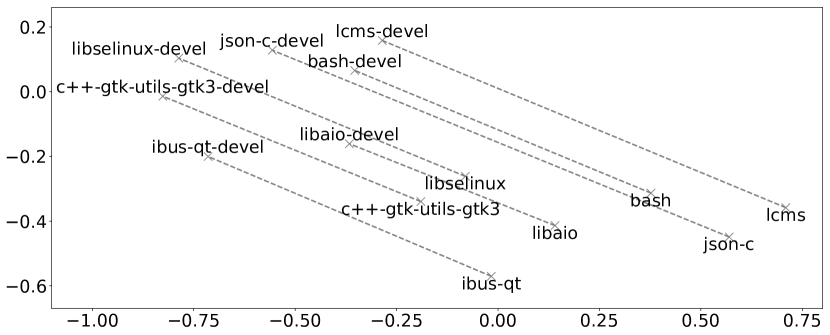
(a) Fedora: “foobar-devel” vs “foobar”

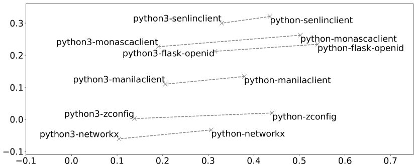
(b) Debian: “python-foobar” vs “python3-foobar”

Figure 2: Illustration of analogies demonstrated in the network embeddings learned using PCTADW-2. Each figure shows a two-dimensional PCA projection of the learned 128-dimensional network embeddings. (a) shows the analogies between development software packages (with their package names ending with “-devel”) and non-development software packages (consisting of executables, libraries, etc.). (b) shows the analogies between Python 2 software packages (with their package names starting with “python-”) and their corresponding Python 3 software packages (with their package names starting with “python3-”) in Debian.

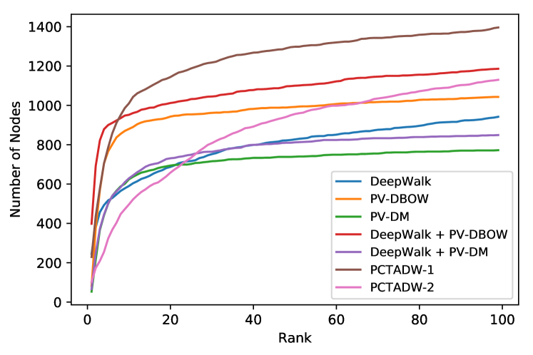
(a) “python-foobar” vs “ruby-foobar” in Debian

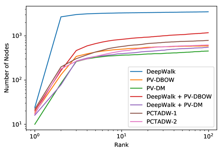
(b) “foobar-devel” vs “foobar” with respect to “bash-devel” vs “bash” in Fedora

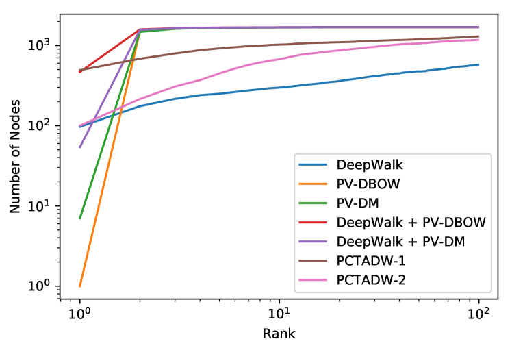
(c) “python-foobar” vs “python3-foobar” with respect to “python-scipy” vs “python3-scipy” in Debian

Figure 3: Results of our analogy tests. Each plot demonstrates one analogy test. The x-axes represent the rank $r_{b}$ and the y-axes represent the number of nodes whose vector representations were ranked below the corresponding rank. Both the x-axes and y-axes in (b) and (c) are in logarithm scales.

Analogies in word embeddings have demonstrated their power for facilitating both algorithmic and human understanding of word embeddings [24, 30]. They have also been used as an empirical instrument for evaluating the quality of word embeddings [24]. In a word embedding, an analogy test asks a question of the form “WordA1 is to WordA2 what WordB1 is to  .” [24] shows two examples: “ ‘Germany’ is to ‘Berlin’ what ‘France’ is to ‘Paris’;” “ ‘quick’ is to ‘quickly’ what ‘slow’ to ‘slowly’.” Mathematically speaking, these mean that $\vec{v}_{\text{Paris}}$ and $\vec{v}_{\text{slowly}}$ are the vectors in the word embedding that are closest (or very close) to $\vec{v}_{\text{Berlin}}-\vec{v}_{\text{Germany}}+\vec{v}_{\text{France}}$ and $\vec{v}_{\text{quickly}}-\vec{v}_{\text{quick}}+\vec{v}_{\text{slow}}$, respectively, where $\vec{v}_{\text{word}}$ is the vector reprensentation of “word.” Unfortunately, to the best of our knowledge, similar analogies have not hitherto been discovered as systematic phenomena in network embeddings or document embeddings. In this subsection, for the first time, we present the systematic presence of analogies in network (and document) embeddings in SPDNs.

Software packages often have analogical semantics associated with themselves. For example, many Python software have both Python 2 and Python 3 versions and they are usually packaged as two different software packages. Therefore, semantically we have the analogy of “Python 2 version of Software A is to its Python 3 version what Python 2 version of Software B is to its Python 3 version.” Similar analogies also exist for software with both Python and Ruby bindings. For another example, many software, especially those written in C or C++, has two separate software packages: One contains the executables and libraries of the software and the other, called a development software package, contains files, such as header files, that are necessary for developing other C/C++ software that uses this software as a depended library. The names of the latter kind of package always end with “-devel” in Fedora and “-dev” in Debian. Figure 2 illustrates these analogies.

We performed two types of analogy tests as follows. In the first type of analogy test, on each dataset, we chose some kinds of analogy pairs, such as aforementioned “foobar-devel” versus “foobar” and “python-foobar” versus “python3-foobar.” Then, for each kind of analogy pair, we considered every two such pairs $(a_{1},a_{2})$ and $(b_{1},b_{2})$. We computed $\vec{v}_{a_{2}}-\vec{v}_{a_{1}}+\vec{v}_{b_{1}}$ and sorted the distances of all vectors in the network embedding to it. We then recorded the rank $r_{b_{2}}$ of $\vec{v}_{b_{2}}$ in these sorted distances. We then compared the cumulative histogram of $r_{b_{2}}$ for the network embedding produced by each algorithm. The taller the histogram is, the better the corresponding network embedding performed for that analogy test. The second type of analogy test is similar to the first type, except that, instead of considering every two pairs $(a_{1},a_{2})$ and $(b_{1},b_{2})$, we only considered all pairs with a specific given pair. For example, for the kind of analogy pair “python-foobar” versus “python3-foobar,” we only compared the cumulative histogram of $r_{b_{2}}$ in case of $(a_{1},a_{2})$ being (“python-scipy”, “python3-scipy”). In this example, we refer to this type of analogy test as “python-foobar” versus “python3-foobar” with respect to “python-scipy” versus “python3-scipy.” We used the second type of analogy test when it would be too computationally expensive if its corresponding analogy test of the first type were performed.

We performed three analogy tests, (a) “python-foobar” versus “ruby-foobar” in Debian, (b) “foobar-devel” versus “foobar” with respect to “bash-devel” versus “bash” in Fedora, and (c) “python-foobar” versus “python3-foobar” with respect to “python-scipy” versus “python3-scipy” in Debian. Figure 3 shows our experimental results. In (a), PCTADW-1 was the winner. In (b), DeepWalk was the winner. In (c), PV-DBOW, PV-DM, PB DeepWalk+PV-DBOW, and DeepWalk+PV-DM won all other three algorithms.

TABLE III: Experimental results of predicting nodes corresponding to development software packages in Fedora using logistic regression. The first column and all numbers mean the same as in Table II.

%		PCTADW-1	PCTADW-2	DeepWalk
5%		0.9400	0.9376	0.8354
10%		0.9426	0.9419	0.8325
20%		0.9451	0.9459	0.8294
25%		0.9463	0.9462	0.8293
33%		0.9468	0.9473	0.8289
50%		0.9476	0.9482	0.8277

Our first observation is that, an algorithm won in node classification did not necessarily win in analogy tests. In other words, an algorithm’s effectiveness in node classification and analogy tests were not necessarily consistent. For example, although PCTADW-1 and PCTADW-2 outperformed other network embedding learning algorithms, they still lost in analogy tests (b) and (c). In fact, Table III briefly shows that both of PCTADW-1 and PCTADW-2 are more effective than DeepWalk in predicting whether a node corresponds to a development package in Fedora.

Our second obversation is that, analogy tests were more responsive to what information had been used for training. In Fedora, a node representing a development software package “foobar-devel” is always directly connected to the node representing “foobar.” This strong relationship in the structure of the network could be the reason that led to the best performance of DeepWalk in (b), since DeepWalk produced network embeddings only based on the structure of the network. Similarly, in Debian, the description of a package “python-foobar” is often almost identical to “python3-foobar” with some “Python” or “Python 2” replaced with “Python 3.” This strong similarity in the documents could be the reason that resulted in the winning of all algorithms involving PV-DBOW and PV-DM in (c). While in (a), neither the structure of the network or documents associated with nodes present a strong relationship. In this case, PCTADW-2 won, perhaps because it has the best integration of the structure of the network and documents associated with nodes.

IX Software Attributes in Network Embeddings

In this section, we demonstrate how we can use the network embeddings of SPDNs for understanding SAs. We show how these network embeddings encapsulate information of SAs and how such information can be further used to understand SAs.

IX-A Encapsulation of Software Attributes

Figure 4: Illustration of the encapsulation of the SA Regular-User/Developer. For visualization purpose, we assume that the dimension of the network embedding is 3. Each cloud represents a reference software package collection. The two dots inside the clouds represent the median vectors of all vector representations in the two collections, respectively. The arrow from $\vec{r}$ to $\vec{s}$ represents the direction that characterizes the SA. The projections of three example software packages zsh, git, and gdb are shown. To help readers visualize, we draw a plane (the gray area) that passes through $(\vec{s}-\vec{r})$.

Regular-User $\longleftarrow$ $\longrightarrow$ Developer

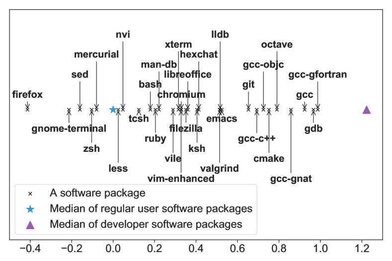
(a) Fedora: Regular-User/Developer

Compiled $\longleftarrow$ $\longrightarrow$ Interpreted

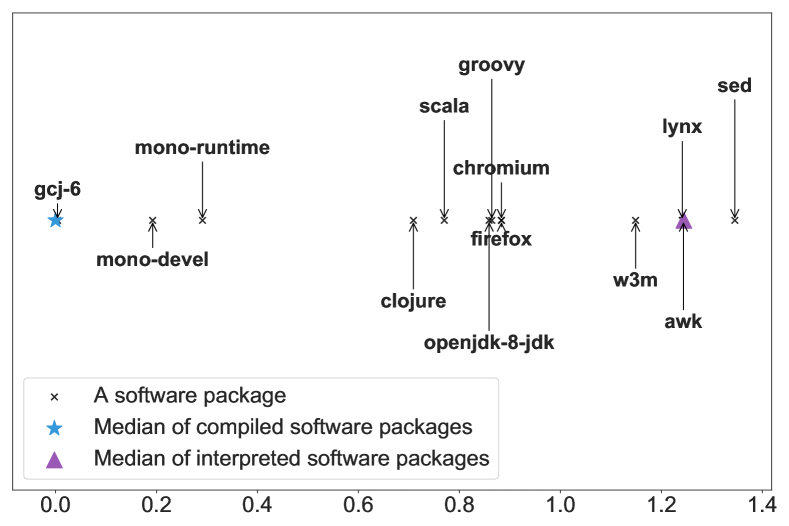
(b) Debian: Compiled/Interpreted

Figure 5: Projected positions of software packages for two SAs. Horizontal axes represent projected positions. Each cross represents a software package, whose name is indicated by an arrow. In each plot, the triangle and star represent opposite extremes of the SA.

In this subsection, we show that a direction in the network embedding space encapsulates information about an SA. We do this by projecting the vector representations of software packages onto individual directions and analyzing their projected positions on them.

IX-A1 Identify a direction for a specific SA using reference software packages

Given an SA, we first select two reference software package collections, each of which comprises software packages that are quintessences of one extreme of this SA. We then use the median vector of all vector representations of software packages in each software package collection to approximate one extreme of this SA. Here, the median vector of a set of vectors $\{\vec{u}_{1},\vec{u}_{2},\ldots\}$ is defined as $\tilde{\vec{u}}=(\tilde{u}^{[1]},\tilde{u}^{[2]},\ldots)$, where each superscript $[\cdot]$ indicates the index of a component of a vector and $\tilde{u}^{[i]}$ is the median of $\{u_{1}^{[i]},u_{2}^{[i]},\ldots\}$ for each $i\in\{1,2,\ldots\}$. We denote these two median vectors by $\vec{r}$ and $\vec{s}$, respectively. The direction along $(\vec{s}-\vec{r})$ can be used to characterize the given SA. Here, the intuition is that the two median vectors are the centroid vectors that best characterize the two extremes of the SA, and linear combinations of these two vectors characterize values of the SA that are in between these two extremes.

For example, let us consider the Regular-User/Developer SA, which characterizes whether a software package is more commonly used by a regular user or a developer. We select two reference software package collections. One consists of software packages that are normally used only by developers, such as python-dev, zsh-dev, and ruby2.3-dev; the other one consists of software packages that are normally used only by regular users, such as inkscape, libreoffice, and thunderbird. In this example, $\vec{r}$ would be the median vector of the former collection and $\vec{s}$ would be the median vector of the latter collection. The direction along $(\vec{s}-\vec{r})$ characterizes the Regular-User/Developer SA.

IX-A2 Analyze vector representations of software packages projected onto the direction along $(\vec{s}-\vec{r})$

We first project the vector representation of each software package onto the direction along $(\vec{s}-\vec{r})$. The projection results in a projected position $(\vec{v_{p}}-\vec{r})\cdot\frac{\vec{s}-\vec{r}}{|\vec{s}-\vec{r}|}$ for the vector representation $\vec{v}_{p}$ of each software package $p$. These projections extract information about the given SA and largely eliminate the influence of other SAs over the vector representations. We can then analyze the given SA through the projected positions: A small projected position indicates closeness to one extreme of the SA and a larger one indicates the other.

Figure 4 illustrates the above steps. As a case study, we performed these steps on two SAs: Regular-user/Developer and Compiled/Interpreted (which characterizes whether a software package is mainly written in a compiled or interpreted programming language). Figure 5 shows the resulting projected positions. We discuss the result of each SA as follows.

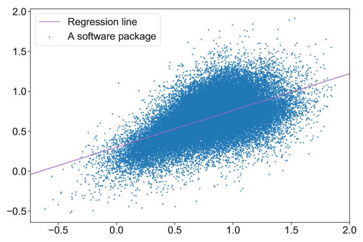
(a)

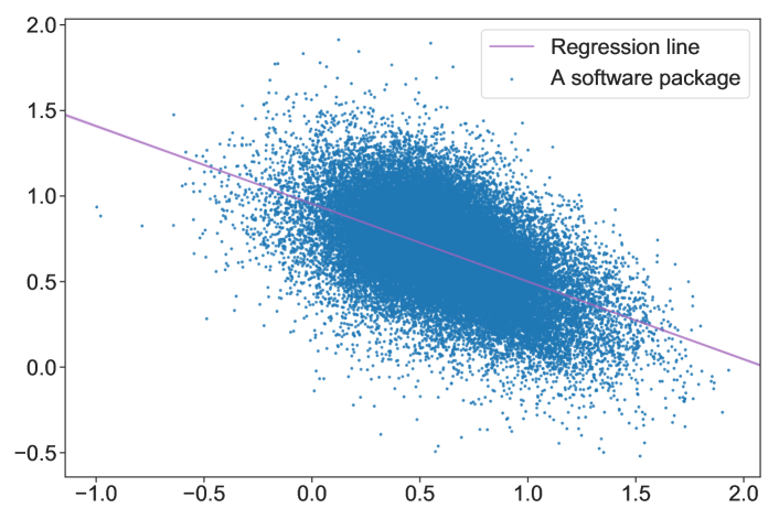
(b)

Figure 6: Illustration of how the knowledge of the correlation between SAs is encapsulated in network embeddings. Each dot represents a software package. The $x$-axes and $y$-axes indicate the projected positions onto the direction of two SAs. The slopes of the regression lines indicate the correlation between the two SAs. A positive slope, like in (a), indicates a positive correlation between the two SAs, and a negative slope, like in (b), indicates a negative correlation. (a): $x$-axis: Regular-User/Developer;$y$-axis: Client/Server. (b): $x$-axis: TUI/GUI; $y$-axis: Client/Server

Regular-User/Developer

We used the Fedora SPDN. In the reference software package collection of Regular-User, we put quintessential non-development software packages, such as thunderbird and inkscape; in the collection of Developer, we put all software packages whose names end with “-devel,” which consist of mostly C/C++ header files.

Figure 5(a) shows the result. We selected the shown software packages because their Regular-User/Developer SAs are representative in terms of their closeness to the two extremes: Some are supposedly close to Regular-User, some are close to Developer, and some are in between. None of them were included in either reference software package collections. With a few exceptions (such as firefox), software packages with small projected positions are generally more commonly used by regular users and those with large projected positions are more commonly used by developers. For example, gcc-c++, cmake, and gdb have larger projected positions because they are commonly used in software development; zsh, sed, and less, have smaller projected positions because they usually serve as system utilities; emacs has a larger projected position than that of vim-enhanced because, in addition to editing programming code, vim-enhanced is also commonly used in system administrative tasks while emacs is not.

Compiled/Interpreted

We used the Debian SPDN. In the reference software package collection of Compiled and Interpreted, we respectively put quintessential compiler software packages, such as go and gcc-c++, and interpreter software packages, such as python and ruby.

Figure 5(b) shows the result. We selected the shown software packages with a criteria similar to that of Fig. 5(a). Small projected positions generally indicate closeness to compilers, and large projected positions indicate closeness to interpreters. For example, all software packages left to groovy provide environments for programming languages that commonly compiled to byte code, which are interpreted during runtime, while those on the right directly interpret programming or markup languages.

IX-B Interactions between Software Attributes

In this subsection, we demonstrate that network embeddings can be leveraged to analyze interactions between SAs. For any two SAs, we do this by statistically measure the relationship between the projected positions of all software packages onto the two corresponding directions.

For every two SAs, similar to the steps in the previous subsection, we first identify the directions of SAs and obtain projected positions onto the two directions for all software packages. We then measure the correlation between the SAs of these software packages using the Pearson correlation coefficient. Each plot in Fig. 6 illustrates the projected positions for all software packages onto the directions of two SAs, and how a regression line indicates the correlation between them.

Table IV summarizes the correlation matrix of various SAs, computed from the projected positions of all software packages onto the directions of these SAs. With the exception of TUI/GUI, the signs of the Pearson correlation coefficients are mostly consistent with human knowledge. For example, Regular-User/Developer and Work/Entertainment are negatively correlated, which is consistent with the fact that software packages for work and not entertainment are more likely to be used by developers than regular users, because work on a GNU/Linux operating system is very often associated with software development. The positive correlation between Regular-User/Developer and Client/Server is consistent with the fact that regular users usually only use software packages that run on the client side and developers also use software packages that run on the server side.

This correlation matrix can also be used to discover unknown and unobvious relationship between SAs. For example, Regular-User/Developer and Compiled/Interpreted are negatively correlated. This is consistent with the fact that 18 out of the 22 most popular development environments as of Feb, 2019 (as reported in [31]) are primarily written in (partially) compiled programming languages, such as Java and C/C++.

TABLE IV: Pearson correlation coefficients between various SAs. Regular, Compiled, TUI, Client, and Work represent SAs Regular-User/Developer, Compiled/Interpreted, TUI/GUI, Client/Server, and Work/Entertainment, respectively. Each cell shows two Pearson correlation coefficients between the SAs of the corresponding row and column for Fedora and Debian, respectively. A positive/negative number indicates a positive/negative correlation. The larger the absolute value of the number is, the stronger the correlation is.

(a) Fedora

	Regular	Compiled	TUI	Client	Work
Regular	1.00	-0.28	0.06	0.26	-0.15
Compiled	-0.28	1.00	0.15	-0.02	0.01
TUI	0.06	0.15	1.00	0.11	0.19
Client	0.26	-0.02	0.11	1.00	0.09
Work	-0.15	0.01	0.19	0.09	1.00

(b) Debian

	Regular	Compiled	TUI	Client	Work
Regular	1.00	-0.42	-0.33	0.55	-0.17
Compiled	-0.42	1.00	-0.21	0.10	0.03
TUI	-0.33	-0.21	1.00	-0.52	0.09
Client	0.55	0.10	-0.52	1.00	-0.10
Work	-0.17	0.03	0.09	-0.10	1.00

X Conclusion and Future Work

In this paper, we presented PCTADW-1 and PCTADW-2, two algorithms for learning embeddings of networks with text-associated nodes, including SPDNs. We extracted two SPDNs from Fedora and Debian. We then demonstrated the effectiveness of PCTADW-1 and PCTADW-2 in comparison with some baselines on these two SPDNs. For the first time, we discovered and discussed the systematic presence of analogies (that are similar to those in word embeddings) in network embeddings. We then demonstrated how we can leverage network embeddings generated from the SPDNs for understanding SAs. We empirically showed that a direction in the network embedding vector space encapsulates information about an SA. We showed that projected positions of software packages on it encode knowledge about the SA of the software package. We finally demonstrated that they can also be used to discover and study interactions and relationship between SAs.

Our work can potentially elicit interesting future research to explore the use of embedding techniques in the research of SE. One direction is to incorporate other metadata of software packages during the training procedure. Another direction is to apply our method for understanding SAs to improve features such as recommendation systems in existing open source software package management systems. Yet another direction is to extend our method to other types of datasets in SE, such as timeline graphs in version control systems.

References

- [1] P. Sen, G. Namata, M. Bilgic, L. Getoor, B. Galligher, and T. Eliassi-Rad, “Collective classification in network data,” AI Magazine, vol. 29, no. 3, pp. 93–106, 2008.
- [2] B. Alipanahi, A. Delong, M. T. Weirauch, and B. J. Frey, “Predicting the sequence specificities of DNA- and RNA-binding proteins by deep learning,” Nature Biotechnology, vol. 33, pp. 831–838, 2015.
- [3] H. Xu, K. Sun, S. Koenig, and T. K. S. Kumar, “A warning propagation-based linear-time-and-space algorithm for the minimum vertex cover problem on giant graphs,” in the International Conference on the Integration of Constraint Programming, Artificial Intelligence, and Operations Research, 2018, pp. 567–584.
- [4] P. Goyal and E. Ferrara, “Graph embedding techniques, applications, and performance: A survey,” Knowledge-Based Systems, vol. 151, pp. 78–94, 2018.
- [5] B. Perozzi, R. Al-Rfou, and S. Skiena, “DeepWalk: Online learning of social representations,” in the ACM SIGKDD International Conference on Knowledge Discovery and Data Mining, 2014, pp. 701–710.
- [6] S. Abu-El-Haija, B. Perozzi, R. Al-Rfou, and A. Alemi, “Watch your step: Learning node embeddings via graph attention,” in Proceedings of the 32nd International Conference on Neural Information Processing Systems, 2018, p. 9198–9208.
- [7] D. Huang, Z. He, Y. Huang, K. Sun, S. Abu-El-Haija, B. Perozzi, K. Lerman, F. Morstatter, and A. Galstyan, “Graph embedding with personalized context distribution,” in Companion Proceedings of the Web Conference 2020, 2020, p. 655–661.
- [8] J. Tang, M. Qu, M. Wang, M. Zhang, J. Yan, and Q. Mei, “LINE: Large-scale information network embedding,” in the International Conference on World Wide Web, 2015, pp. 1067–1077.
- [9] A. Grover and J. Leskovec, “node2vec: Scalable feature learning for networks,” in the ACM SIGKDD International Conference on Knowledge Discovery and Data Mining, 2016, pp. 855–864.
- [10] S. Cao, W. Lu, and Q. Xu, “Deep neural networks for learning graph representations,” in the AAAI Conference on Artificial Intelligence, 2016, pp. 1145–1152.
- [11] Y. Dong, N. V. Chawla, and A. Swami, “Metapath2vec: Scalable representation learning for heterogeneous networks,” in the ACM SIGKDD International Conference on Knowledge Discovery and Data Mining, 2017, pp. 135–144.
- [12] X. Wang, P. Cui, J. Wang, J. Pei, W. Zhu, and S. Yang, “Community preserving network embedding,” in the AAAI Conference on Artificial Intelligence, 2017, pp. 203–209.
- [13] Y.-A. Lai, C.-C. Hsu, W. H. Chen, M.-Y. Yeh, and S.-D. Lin, “PRUNE: Preserving proximity and global ranking for network embedding,” in the Neural Information Processing Systems Conference, 2017, pp. 5257–5266.
- [14] W. Hamilton, Z. Ying, and J. Leskovec, “Inductive representation learning on large graphs,” in the Neural Information Processing Systems Conference, 2017, pp. 1024–1034.
- [15] X. Huang, J. Li, and X. Hu, “Label informed attributed network embedding,” in the ACM International Conference on Web Search and Data Mining, 2017, pp. 731–739.
- [16] Z. Wang, X. Ye, C. Wang, Y. Wu, C. Wang, and K. Liang, “RSDNE: Exploring relaxed similarity and dissimilarity from completely-imbalanced labels for network embedding,” in the AAAI Conference on Artificial Intelligence, 2018, pp. 475–482.
- [17] Q. Dai, Q. Li, J. Tang, and D. Wang, “Adversarial network embedding,” in The Thirty-Second AAAI Conference on Artificial Intelligence), 2018, pp. 2167–2174.
- [18] J. Sun, B. Bandyopadhyay, A. Bashizade, P. Sadayappan, and S. Parthasarathy, “ATP: directed graph embedding with asymmetric transitivity preservation,” in The Thirty-Third AAAI Conference on Artificial Intelligence, 2019, pp. 265–272.
- [19] J. Kim, H. Park, J.-E. Lee, and U. Kang, “SIDE: Representation learning in signed directed networks,” in the World Wide Web Conference, 2018, pp. 509–518.
- [20] C. Yang, Z. Liu, D. Zhao, M. Sun, and E. Chang, “Network representation learning with rich text information,” in the International Joint Conference on Artificial Intelligence, 2015, pp. 2111–2117.
- [21] S. Ganguly and V. Pudi, “Paper2vec: Combining graph and text information for scientific paper representation,” in the European Conference on Information Retrieval, 2017, pp. 383–395.
- [22] A. Shatnawi, H. Mili, G. E. Boussaidi, A. Boubaker, Y.-G. Guéhéneuc, N. Moha, J. Privat, and M. Abdellatif, “Analyzing program dependencies in Java EE applications,” in the International Conference on Mining Software Repositories, 2017, pp. 64–74.
- [23] A. Decan, T. Mens, and E. Constantinou, “On the impact of security vulnerabilities in the npm package dependency network,” in the International Conference on Mining Software Repositories, 2018, pp. 181–191.
- [24] T. Mikolov, I. Sutskever, K. Chen, G. Corrado, and J. Dean, “Distributed representations of words and phrases and their compositionality,” in the Neural Information Processing Systems Conference, 2013.
- [25] Q. Le and T. Mikolov, “Distributed representations of sentences and documents,” in the International Conference on Machine Learning, vol. 32, no. 2, 2014, pp. 1188–1196.
- [26] Y. Fisher, “Red Hat Enterprise Linux builds the foundation for the world’s fastest supercomputer(s),” https://www.redhat.com/en/blog/red-hat-enterprise-linux-builds-foundation-worlds-fastest-supercomputers, 2018, accessed: 2018-09-05.
- [27] M. Gelbmann, “Ubuntu became the most popular Linux distribution for web servers,” https://w3techs.com/blog/entry/ubuntu_became_the_most_popular_linux_distribution_for_web_servers, 2016, accessed: 2018-09-05.
- [28] R. Řehůřek and P. Sojka, “Software framework for topic modelling with large corpora,” in the LREC 2010 Workshop on New Challenges for NLP Frameworks, 2010, pp. 45–50.
- [29] D. P. Kingma and J. L. Ba, “Adam: A method for stochastic optimization,” in the International Conference on Learning Representations, 2015.
- [30] J. Pennington, R. Socher, and C. D. Manning, “GloVe: Global vectors for word representation,” in the Conference on Empirical Methods in Natural Language Processing, 2014, pp. 1532–1543.
- [31] “Developer survey results 2019,” https://insights.stackoverflow.com/survey/2019, 2019.