Multi-Source Domain Adaptation with Mixture of Experts

Abstract

We propose a mixture-of-experts approach for unsupervised domain adaptation from multiple sources. The key idea is to explicitly capture the relationship between a target example and different source domains. This relationship, expressed by a point-to-set metric, determines how to combine predictors trained on various domains. The metric is learned in an unsupervised fashion using meta-training. Experimental results on sentiment analysis and part-of-speech tagging demonstrate that our approach consistently outperforms multiple baselines and can robustly handle negative transfer.

1 Introduction

Typical domain adaptation methods are designed to transfer supervision from a single source domain. However, in many practical applications, we have access to multiple sources. For instance, in sentiment analysis of product reviews, we can often transfer from a wide range of product domains, rather than one. This can be particularly promising for target domains which do not match any one available source well. For example, the Kitchen product domain may include reviews on pans, cookbooks or electronic devices, which cannot be perfectly aligned to a single source such as Cookware, Books or Electronics. By intelligently aggregating distinct and complementary information from multiple sources, we may be able to better fit the target distribution.

A straightforward approach to utilizing data from multiple sources is to combine them into a single domain. This strategy, however, does not account for distinct relations between individual sources and the target example. Constructing a common feature space for this heterogeneous collection may wash out informative characteristics of individual domains and also lead to negative transfer Rosenstein et al. (2005).

Therefore, we propose to explicitly model the relationship between different source domains and target examples. We hypothesize that different source domains are aligned to different sub-spaces of the target domain. Specifically, in this paper, we model the domain relationship with a mixture-of-experts (MoE) approach Jacobs et al. (1991b). For each target example, the predicted posterior is a weighted combination of all the experts’ predictions. The weights reflect the proximity of the example to each source domain. Our model learns this point-to-set metric automatically, without additional supervision.

We define the point-to-set metric using Mahalanobis distance Weinberger and Saul (2009) between individual examples and a set (i.e. domain), which are computed within the hidden representation space of our model. The main challenge is to learn this metric in an unsupervised setting. We address it through a meta-training procedure, in which we create multiple meta-tasks of domain adaptation from the source domains. In each meta-task, we pick one of the source domains as meta-target, and the rest source domains as meta-sources. By minimizing the loss using the MoE predictions on meta-target, we are able to learn both the model and the metric simultaneously. To further improve transfer quality, we align the encoding space of our target and source domains via adversarial learning.

We evaluate our approach on sentiment analysis using the benchmark multi-domain Amazon reviews dataset Chen et al. (2012); Ziser and Reichart (2017) as well as on part-of-speech (POS) tagging using the SANCL dataset Petrov and McDonald (2012). Experiments show that our approach consistently improves the adaptation results over the best single-source model and a unified multi-source model. On average, we achieve a 7% relative error reduction on the Amazon reviews dataset, and a 13% on the SANCL dataset. Importantly, the POS tagging experiments on the SANCL dataset demonstrate that our method is able to robustly handle negative transfer from unrelated sources (e.g., Twitter) and utilize it effectively to consistently improve performance.

2 Related Work

Unsupervised domain adaptation

Most existing domain adaptation methods focus on aligning the feature space between source and target domains to reduce the domain shift Ben-David et al. (2007); Blitzer et al. (2007, 2006); Pan et al. (2010). Our approach is close to the representation learning approaches, such as the denoising autoencoder Glorot et al. (2011), the marginalized stacked denoising autoencoders Chen et al. (2012), and domain adversarial networks Tzeng et al. (2014); Ganin et al. (2016); Zhang et al. (2017); Shen et al. (2018).

In contrast to these previous approaches, however, our approach not only learns a shared representation space that generalizes well to the target domain, but also captures informative characteristics of individual source domains.

Multi-Source domain adaptation

The main challenge in using multiple sources for domain adaptation is in learning domain relations. Some approaches assume that all source domains are equally important to the target domain Li and Zong (2008); Luo et al. (2008); Crammer et al. (2008). Others learn a global domain similarity metric using labeled data in a supervised fashion Yang et al. (2007); Duan et al. (2009); Yu et al. (2018) or use predefined similarity measures Ruder et al. (2017). Alternatively, Mansour et al. (2009) and Bhatt et al. (2016) utilize unlabeled data of the target domain to find a distribution weighted combination of the source domains or to construct an auxiliary training set of the source domain instances close to the target domain instances. Recent adversarial methods on multi-source domain adaptation Zhao et al. (2018); Chen and Cardie (2018) align source domains to the target domains globally, without accounting for the distinct importance of each source with respect to a specific target example.

Beyond the global domain-to-domain relations, Ruder and Plank (2017) use example-to-domain similarity measures to select data from multiple sources for a specific target domain, which are then combined to train a single classifier. The work most related to ours is by Kim et al. (2017). They also model the example-to-domain relations, but use an attention mechanism. The attention module is learned using limited training data from the target domain in a supervised fashion. Our method, however, works in an unsupervised setting without utilizing any labeled data from the target domain.

3 Methodology

Problem definition

We follow the unsupervised multi-source domain adaptation setup, assuming access to labeled training data from $K$ source domains: $\{\mathcal{S}_{i}\}_{i=1}^{K}$ where $\mathcal{S}_{i}\triangleq\{(x_{t}^{\mathcal{S}_{i}},y_{t}^{\mathcal{S}_{i}})\}_{t=1}^{\left|\mathcal{S}_{i}\right|}$, and (optionally) unlabeled data from a target domain: $\mathcal{T}\triangleq\{x_{t}^{\mathcal{T}}\}_{t=1}^{\left|\mathcal{T}\right|}$. The goal is to learn a model using the source domain data, that generalizes well to the target domain.

Notations

For the rest of the paper, we denote an individual example as $x$, and a batch of examples as $\mathbf{x}$. We use superscript to denote the domain from which an example is sampled, and use subscript to denote the index of an example.

3.1 Overview of Our Approach

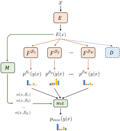
Figure 1: Architecture of the MoE model. $E$ is the encoder which maps an input $x$ to a hidden representation $E(x)$; $F^{\mathcal{S}_{i}}$ is the classifier on the $i^{th}$ source domain; $D$ is the critic that is only used during adversarial training. $M$ is the metric learning component, which takes the encoding of $x$ and source domains ($\mathcal{S}_{1:K}$) as input and computes $\alpha$.

We model the multiple source domains as a mixture of experts, and learn a point-to-set metric $\alpha$ to weight the experts for different target examples. The metric is learned in an unsupervised manner.

Our model consists of four key components as shown in Figure 1, namely the encoder ($E$), classifier ($F$), metric ($M$) and adversary ($D$). We use a typical neural multi-task learning architecture Caruana (1997), with a shared encoder across all sources, and domain-specific classifiers ($\{F^{\mathcal{S}_{i}}\}_{i=1}^{K}$). Each input is first encoded with $E$, and then fed to each classifier to obtain the domain-specific predictions (i.e. posteriors). The final predictions are then weighted based on the metric (see Equation 1).

We start by describing the representation learning component.

3.2 Representation

Our goal is to design an encoder that supports transfer, while maintaining source domain-specific information. Depending on different tasks and datasets, we select appropriate encoders — multilayer perceptron (MLP), convolutional neural network (CNN) or long short-term memory networks (LSTM) (see Section 4.3 for details).

We further add an adversarial module ($D$) on top of the encoder, in order to align the target domain with the sources. $D$ is typically designed as a parameterized classifier in domain adversarial networks Ganin et al. (2016); Zhang et al. (2017), which is trained jointly with the encoder and the classifiers through a minimax game. Here, we instead use Maximum Mean Discrepancy (MMD) Gretton et al. (2012) as our adversary. This distance metric measures the discrepancy between two distributions explicitly in a non-parametric manner, greatly simplifying the training procedure compared to domain adversarial networks which use an additional domain classifier module.

3.3 Mixture of Experts

Given an example $x$ from the target domain, we model its posterior distribution as a mixture of posteriors produced by models trained on different source domain data:

$$\begin{split}p_{moe}(y|x)&=\sum_{i=1}^{K}\alpha(x,\mathcal{S}_{i})\cdot p^{\mathcal{S}_{i}}(y|x)\\ &=\sum_{i=1}^{K}\alpha(x,\mathcal{S}_{i})\cdot\mathtt{softmax}\big{(}\mathbf{W}^{\mathcal{S}_{i}}E(x)\big{)}\end{split}$$ (1)

$p^{\mathcal{S}_{i}}$ is the posterior distribution produced by the $i^{th}$ source classifier $F^{\mathcal{S}_{i}}$ (the $i^{th}$ expert). $\mathbf{W}^{\mathcal{S}_{i}}$ is the output layer weights of $F^{\mathcal{S}_{i}}$, $\alpha$ is a parameterized metric function that measures how much confidence we put in the specific source expert for a given example $x$. To derive $\alpha$, we first define a point-to-set Mahalanobis distance metric between an example $x$ and a set $\mathcal{S}$:

$$d(x,\mathcal{S})=\Big{(}\big{(}E(x)-\mu^{\mathcal{S}}\big{)}^{\top}\mathbf{M}^{\mathcal{S}}\big{(}E(x)-\mu^{\mathcal{S}}\big{)}\Big{)}^{\frac{1}{2}}$$

where $\mu^{\mathcal{S}}$ is the mean encoding of $\mathcal{S}$. In its original form, the matrix $\mathbf{M}^{\mathcal{S}}$ played the role of the inverse covariance matrix. However, computing the inverse of the covariance matrix is both time consuming and numerically unstable in practice. Here we allow $\mathbf{M}$ to denote any positive semi-definite matrix which is to be estimated during training Weinberger and Saul (2009). To guarantee the positive semi-definiteness of $\mathbf{M}$, we approximate $\mathbf{M}$ with $\mathbf{M}=\mathbf{U}\mathbf{U}^{\top}$, where $\mathbf{U}\in\mathbb{R}^{h\times r}$, $h$ is the dimension of hidden representations and $r$ is a hyper-parameter controlling the rank of $\mathbf{M}$.

Based on the distance metric, we further derive a confidence score $e(x,\mathcal{S}_{i})=f\big{(}d(x,\mathcal{S}_{i})\big{)}$ for each specific expert. The final metric values $\alpha(x,\mathcal{S}_{i})$ are then obtained by normalizing these confidence scores:

$$\alpha(x,\mathcal{S}_{i})=\frac{\exp\big{(}e(x,\mathcal{S}_{i})\big{)}}{\sum_{j=1}^{K}\exp\big{(}e(x,\mathcal{S}_{j})\big{)}}$$ (2)

Here, we explain our design of $e(x,\mathcal{S})$ on two tasks, respectively binary classification and sequence tagging, which are also used for evaluation in this paper (Section 4).

Binary classification

The point-to-set Mahalanobis distance metric measures the distance between an example $x$ and the mean encoding of $\mathcal{S}$, i.e. $\mu^{\mathcal{S}}$, while taking into account the (pseudo) covariance of $\mathcal{S}$. In binary classification, however, the mean vector $\mu^{\mathcal{S}}$ is likely to be located near the decision boundary, particularly under a balanced setting. Therefore, a small $d(x,\mathcal{S})$ actually implies lower confidence of the corresponding classifier, which is counter-intuitive. To this end, we instead define the confidence $e(x,\mathcal{S})$ as the difference between the distances from $x$ to each category of $\mathcal{S}$, referred to as Maximum Cluster Difference in Ruder et al. (2017):

$$e(x,\mathcal{S})=\left|d(x,\mathcal{S}^{+})-d(x,\mathcal{S}^{-})\right|$$

Here $\mathcal{S}^{+}$ and $\mathcal{S}^{-}$ stand for the positive space and negative space of $\mathcal{S}$ respectively. Consequently, if $x$ is either far away from $\mathcal{S}$ (i.e., $x$ is not in the manifold of $\mathcal{S}$) or near the classification boundary, we will get a small $e(x,\mathcal{S})$ indicating a low confidence to the corresponding prediction. On the contrary, if $x$ is much closer to a specific category of $\mathcal{S}$ than other categories, the classifier will get a higher confidence.

Sequence tagging

For sequence tagging tasks (e.g., POS tagging), we compute the distance metric at the token level. Unlike in binary classification, the decision boundary here is more complicated, and the label distribution is typically imbalanced. The mean vector $\mu^{\mathcal{S}}$ is unlikely to be located at the decision boundary. So we directly use the (reverse) distance as the confidence value for each token $x$:

$$e(x,\mathcal{S})=-d(x,\mathcal{S})$$

3.4 Training

Since we do not have annotated data in the target domain, we have to learn our model in an unsupervised fashion. Inspired by the recent progress on few-shot learning with metric-based models such as matching network Vinyals et al. (2016); Yu et al. (2018) and prototypical network Snell et al. (2017), we propose the following meta-training approach. Given $K$ source domains, each source domain will be considered as a target, referred to as meta-target, with the rest of the source domains as meta-sources. This way, we obtain $K$ (meta-sources, meta-target) training pairs for domain adaptation. Then, we apply our MoE formulation over these meta-training pairs to learn the metric. At testing time, the metric will be applied to all the $K$ source domains for each example in the target domain.

We optimize two main objectives: the MoE objective and the multi-task learning (MTL) objective.

MoE objective

For each example in each meta-target domain, we compute its MoE posterior using the corresponding meta-sources. Therefore, we get the following MoE loss over the entire multi-source training data:

$$\begin{split}\mathcal{L}_{moe}&=-\sum_{i=1}^{K}\sum_{j=1}^{\left|\mathcal{S}_{i}\right|}\log p_{moe}(y^{\mathcal{S}_{i}}_{j}|x^{\mathcal{S}_{i}}_{j})\\ &=-\sum_{i=1}^{K}\sum_{j=1}^{\left|\mathcal{S}_{i}\right|}\log\sum_{l=1,l\neq i}^{K}\alpha(x,\mathcal{S}_{l})\cdot p^{\mathcal{S}_{l}}(y^{\mathcal{S}_{i}}_{j}|x^{\mathcal{S}_{i}}_{j})\end{split}$$ (3)

Note that $\alpha$ is normalized over the meta-sources for each meta-target, rather than over all the $K$ sources.

MTL objective

For each meta-target, we further optimize a supervised cross-entropy loss using the corresponding labels. All supervised objectives are optimized jointly with the encoder being shared, resulting in the following multi-task learning objective:

$$\mathcal{L}_{mtl}=-\sum_{i=1}^{K}\sum_{j=1}^{\left|\mathcal{S}_{i}\right|}\log p^{\mathcal{S}_{i}}(y^{\mathcal{S}_{i}}_{j}|x^{\mathcal{S}_{i}}_{j})$$ (4)

Algorithm 1 Training Procedure

1:Input: multi-source domain data $\mathcal{S}=\{\mathcal{S}_{i}\}_{i=1}^{K}$, target domain data $\mathcal{T}$

2:Hyper-parameters: mini-batch size $m$, coefficients for different losses: $\lambda$, $\gamma$ and $\eta$

3:repeat

4:     Sample $K$ source mini-batches $\{(\mathbf{x}^{\mathcal{S}_{i}},\mathbf{y}^{\mathcal{S}_{i}})\}_{i=1}^{K}$ from $\mathcal{S}$ and a target mini-batch $\mathbf{x}^{T}$ from $\mathcal{T}$

5:     $\mathcal{L}_{mtl},\mathcal{L}_{moe},\mathcal{L}_{adv},\mathcal{R}_{h}\leftarrow 0$

6:     for $t=1$ to $K$ do

7:         Set meta-target as $\mathcal{T}^{meta}\triangleq\tilde{\mathcal{S}}_{t}\triangleq(\mathbf{x}^{\mathcal{S}_{t}},\mathbf{y}^{\mathcal{S}_{t}})$

8:         Set meta-sources as $\mathcal{S}^{meta}\triangleq\{\tilde{\mathcal{S}}_{i}\}_{i=1,i\neq t}^{K}$, where $\tilde{\mathcal{S}}_{i}\triangleq(\mathbf{x}^{\mathcal{S}_{i}},\mathbf{y}^{\mathcal{S}_{i}})$

9:         Compute cross-entropy loss over $\mathcal{T}^{meta}$, and add to $\mathcal{L}_{mtl}$

10:         Compute Mahalanobis metric $\alpha(x,\mathcal{S}^{\prime})$ for each $x\in\mathcal{T}^{meta}$ and $\mathcal{S}^{\prime}\in\mathcal{S}^{meta}$ $\triangleright$ Eq. (2)

11:         Compute MoE loss over ($\mathcal{S}^{meta}$, $\mathcal{T}^{meta}$) using $\bm{\alpha}$, and add to $\mathcal{L}_{moe}$ $\triangleright$ Eq. (3)

12:         Compute entropy of $\bm{\alpha}(x,\cdot)$ for each $x\in\mathcal{T}^{meta}$, and add to $\mathcal{R}_{h}$ $\triangleright$ Eq. (6)

13:     end for

14:     Compute MMD between $\mathbf{x}^{\mathcal{T}}$ and $\cup_{i=1}^{K}\mathbf{x}^{\mathcal{S}_{i}}$, and add to $\mathcal{L}_{adv}$ $\triangleright$ Eq. (5)

15:     Update parameters via backpropagating gradients of the total loss $\mathcal{L}$ $\triangleright$ Eq. (7)

16:until converge

Adversary-augmented MoE

We use MMD Gretton et al. (2012) as the adversary to minimize the divergence between the marginal distribution of target domain and source domains. Specifically, at each training epoch, given the $K$ batches $\{\mathbf{x}^{\mathcal{S}_{1}},\mathbf{x}^{\mathcal{S}_{2}},...,\mathbf{x}^{\mathcal{S}_{K}}\}$ from all the source domains, we sample a batch (unlabeled) $\mathbf{x}^{\mathcal{T}}$ from our target domain, and minimize the MMD:

$$\mathcal{L}_{adv}=\mathtt{MMD}^{2}(\mathbf{x}^{\mathcal{S}_{1}}\cup...\cup\mathbf{x}^{\mathcal{S}_{K}},\mathbf{x}^{\mathcal{T}})$$ (5)

where

$$\begin{split}&\mathtt{MMD}(\mathcal{D}^{\mathcal{S}},\mathcal{D}^{\mathcal{T}})=\\ &\left\|\frac{1}{|\mathcal{D}^{\mathcal{S}}|}\sum_{x_{s}\in\mathcal{D}^{\mathcal{S}}}\phi\big{(}E(x_{s})\big{)}-\frac{1}{|\mathcal{D}^{\mathcal{T}}|}\sum_{x_{t}\in\mathcal{D}^{\mathcal{T}}}\phi\big{(}E(x_{t})\big{)}\right\|_{\mathcal{H}}\end{split}$$

measures the discrepancy between $\mathcal{D}^{\mathcal{S}}$ and $\mathcal{D}^{\mathcal{T}}$ based on Reproducing Kernel Hilbert Space (RKHS). $\phi(\cdot)$ is the feature map induced by a universal kernel. We follow Bousmalis et al. (2016) and use a linear combination of multiple RBF kernels: $\kappa(\bm{h}_{i},\bm{h}_{j})=\Sigma_{n}\exp(-\frac{1}{2\sigma_{n}}\left\|\bm{h}_{i}-\bm{h}_{j}\right\|^{2})$.

Entropy regularization

In the meta-training process, for each example $x$ in meta-target, we know exactly from which source $x$ is sampled. This provides additional insight that the $\alpha$ distribution is skewed, which can be utilized as a soft constraint. Therefore, we propose to regularize the entropy of the $\alpha$ distribution over all the sources, rather than meta-sources:

$$H\big{(}\bm{\alpha}(x,\cdot)\big{)}=-\sum_{l=1}^{K}\mathbf{\alpha}(x,\mathcal{S}_{l})\cdot\log\mathbf{\alpha}(x,\mathcal{S}_{l})$$

$$\mathcal{R}_{h}=\sum_{i=1}^{K}\sum_{j=1}^{\left|\mathcal{S}_{i}\right|}H\big{(}\bm{\alpha}(x^{\mathcal{S}_{i}}_{j},\cdot)\big{)}$$ (6)

Joint learning

Our final objective is the weighted combination of each individual component loss:

$$\begin{split}\mathcal{L}=&~{}\lambda\cdot\mathcal{L}_{moe}+(1-\lambda)\cdot\mathcal{L}_{mtl}\\ &+\gamma\cdot\mathcal{L}_{adv}\\ &+\eta\cdot\mathcal{R}_{h}\end{split}$$ (7)

where $\lambda$ controls the balance of the MoE loss and MTL loss. $\gamma$ is set to 0 in non-adversarial setting when unlabeled data from the target domain is not provided. Additionally, it would be straightforward to add an MoE loss for labeled data in the target domain if they are available, thus extending our framework to a setting where we have few-shot target annotations. The training process is shown in Algorithm 1.

4 Experimental Setup

4.1 Task and Dataset

Sentiment classification

We use the multi-domain Amazon reviews dataset Blitzer et al. (2007), one of the standard benchmark datasets for domain adaptation. It contains reviews on four domains: Books (B), DVDs (D), Electronics (E), and Kitchen appliances (K).

We follow the specific experiment settings proposed by Chen et al. (2012) (Chen12) and Ziser and Reichart (2017) (Ziser17).

1. In Chen12, each domain has 2,000 labeled examples for training (1,000 positive and 1,000 negative), and the target test set has 3,000 to 6,000 examples.

2. In Ziser17, each domain also has 2,000 labeled examples (1,000 positive and 1,000 negative), sampled differently from Chen12.

For each dataset, we conduct experiments by selecting the target domain in a round-robin fashion. Following the protocol in previous work, we use cross-validation over source domains for hyper-parameters selection for each adaptation task Zhao et al. (2018). When training with an adversary, we use the 2,000 examples training set of the target domain as the unlabeled data in both the settings. In Ziser17, the same data is also used for test, resulting in a transductive setting.

Part-of-Speech tagging

We further consider a sequence tagging task, where the metric is computed over the token-level encodings and multi-class predictions are made at the token (word) level. We use the SANCL dataset Petrov and McDonald (2012) which contains part-of-speech (POS) tagging annotations in 5 web domains: Emails, Weblogs, Answers, Newsgroups, and Reviews. Among these, Newsgroups, Reviews, and Answers have both a validation and a test set, and are used as target domains. The test set from Weblogs and Emails are used as individual source domains. The tagging is performed using the Universal POS tagset Petrov et al. (2012). We also use Twitter Liu et al. (2018) as an additional training source. Since it differs substantially from other sources and the target domain, we can assess our model’s ability to handle negative transfer. We consider 750 sentences from each SANCL source domain for training, and up to 2,250 sentences from the Twitter dataset to magnify the negative transfer. The validation set in the standard split of each target domain is used for hyper-parameters selection and early-stopping in our experiments.

4.2 Baselines

We verify the efficacy of our approach (MoE) in non-adversarial and adversarial settings respectively. In both settings, we compare our approach against the following two baselines:

• best-SS: the best single-source adaptation model among all the sources.

• uni-MS: the unified multi-source adaptation model, which is trained using the combination of all the source domain data with single-source transfer methods. uni-MS is a common and strong baseline for multi-source domain adaptation Zhao et al. (2018).

For the rest of the paper, we name the adversarial counterpart of the models as $*$-A.

In the adversarial setting on Chen12, in addition to best-SS and uni-MS with adversarial loss, we further compare with the following two systems that also utilize unlabeled data from target domain.

• mSDA: the marginalized stacked denoising autoencoder Chen et al. (2012). mSDA outperforms prior deep learning and shallow learning approaches such as structural correspondence learning Blitzer et al. (2007) and denoising autoencoder Glorot et al. (2011).

• MDAN: the multi-source domain adversarial network Zhao et al. (2018). MDAN gives the state-of-the-art performance for multi-source domain adaptation on Chen12. It generalizes the domain adversarial network to multiple source domain adaptation by selectively backpropagating the domain discrimination loss according to domain classification error.

4.3 Implementation Details

For Chen12, since the dataset is in TF-IDF format and the word ordering information is not available, we use a multilayer perceptron with an input layer of 5,000 dimensions and one hidden layer of 500 dimensions as our encoder. For Ziser17, we instead use a convolutional neural network encoder with a combination of kernel widths 3 and 5 Kim (2014), each with one hidden layer of size 150, which are then concatenated to a 300 dimension representation.

For the POS tagging encoder, we use a hierarchical bidirectional LSTM (BiLSTM) network, which contains a character-level BiLSTM for generating individual word representations, followed by a word-level BiLSTM that generates contextualized word representations.

For MMD, we follow Bousmalis et al. (2016) and use 19 RBF kernels with the standard deviation parameters ranging from $10^{-6}$ to $10^{6}$.

Setting	Non-adversarial			adversarial
	best-SS	uni-MS	MoE	mSDA†	MDAN	best-SS-A	uni-MS-A	MoE-A
D,E,K–B	75.43	78.43	79.42	76.98	78.63	80.07	80.25	80.87
B,E,K–D	81.23	82.49	83.35	78.61	80.65	82.68	83.30	83.99
B,D,K–E	85.51	84.79∗	86.62	81.98	85.34	86.32	85.96∗	86.38
B,D,E–K	86.83	87.00	87.96	84.33	86.26	87.05	87.55	88.06
Average	82.25	83.18	84.34	80.48	82.72	84.03	84.27	84.83

Table 1: Multi-Source domain adaptation accuracy on Amazon dataset of Chen12. ^∗ indicates negative transfer, i.e., the unified multi-source model underperforms the best single-source model. mSDA^† is not an adversarial approach, but utilizes unlabeled data from target domain.

Setting	Non-adversarial			adversarial
	best-SS	uni-MS	MoE	best-SS-A	uni-MS-A	MoE-A
D,E,K–B	85.35	87.00	87.55	86.85	87.55	87.85
B,E,K–D	85.25	86.80	87.85	86.00	87.40	87.65
B,D,K–E	86.80	88.30	89.20	88.90	89.35	89.50
B,D,E–K	88.90	89.65	90.45	89.95	90.35	90.45
Average	86.58	87.94	88.76	87.93	88.66	88.86

Table 2: Multi-Source domain adaptation accuracy on Amazon dataset of Ziser17.

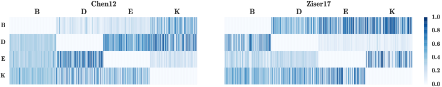
Figure 2: $\alpha$ distributions across source domains for randomly selected 200 examples in each target domain of Chen12 (left) and Ziser17 (right). Columns represent target domains and rows represent sources.

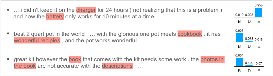
Figure 3: Examples of Kitchen (K) reviews in Ziser17 and their $\alpha$ distribution over Books (B), DVDs (D) and Electronics (E). The manually highlighted words indicate the specific Kitchen products described in the reviews.

All the models were trained using Adam with weight decay. Learning rate is set to $10^{-4}$ for Chen12 and $10^{-3}$ for Ziser17 and POS tagging. We use mini-batches of 32 samples from each domain. We tune the coefficients $\lambda$, $\eta$ for each adaptation task. $\gamma$ is set to 1 for all experiments.

5 Results

5.1 Sentiment Analysis on Amazon Reviews

We report our results on the Amazon reviews datasets in Table 1 (Chen12) and Table 2 (Ziser17). Our approach (MoE) consistently achieves the best performance across different settings and tasks.

The results clearly demonstrate the value of using multiple sources. In most cases, even a unified model performs better than the oracle best single source. By smartly combining all the sources, our model outperforms the unified model significantly. One exception is the task of “B,D,K-E” in Chen12, where the unified multi-source model doesn’t improve over the best single source model, constituting a negative transfer scenario. However, even in this scenario, our approach still performs significantly better, demonstrating its robustness in handling negative transfer.

Impact of adversarial adaptation

We achieve consistent improvements over the baseline systems with the addition of the adversarial loss. In most cases, MoE also achieves additional improvement (e.g., 79.42% vs. 80.87% in “D,E,K-B”). We notice that in some cases, e.g., “B,D,K-E” in Chen12 and “B,E,K-D” in Ziser17, the adversarial loss doesn’t help MoE. This might be attributed to the fact that by aligning the target distribution with the source domains, the representation space becomes more compact, thus making it more difficult to capture source domain-specific characteristics and increasing the difficulty of metric learning in MoE.

Analysis on the metric ($\alpha$)

Figure 2 visualizes the distribution of $\alpha$ values, learned by our model in different tasks, across the source domains. The visualization is based on 200 examples for each domain randomly sampled from the corresponding test set. From the heatmap we can see that for a specific target domain, different examples may have different $\alpha$ distributions. Moreover, for most examples, the $\alpha$ distribution is skewed, indicating that our model draws on a few most informative source domains.

Figure 3 exemplifies the above point. For instance, the first review about “charger” and “battery” is closer to the Electronics source domain. This relation is successfully captured by the $\alpha$ distribution produced by our model.

Setting	Chen12 (w/o $\mathcal{R}_{h}$)		Ziser17 (w/o $\mathcal{R}_{h}$)
	MoE	MoE-A	MoE	MoE-A
D,E,K–B	-0.70	-0.51	-0.75	-0.60
B,E,K–D	-0.67	-0.41	-0.05	-1.20
B,D,K–E	-1.93	-0.44	-0.70	-0.60
B,D,E–K	-0.49	-0.09	-0.50	+0.30

Table 3: Ablation test of entropy regularizer on Chen12 and Ziser17 (decrease in accuracy).

We further investigate the impact of entropy regularization over $\alpha$. Table 3 summarizes the ablation test results of entropy regularization ($\eta=0$) on Chen12 and Ziser17. It shows that entropy regularization benefits our model under both non-adversarial and adversarial settings.

Target	Non-adversarial				adversarial
	best-SS	uni-MS	uni-MS†	MoE	best-SS-A	uni-MS-A	uni-MS-A†	MoE-A
Answers	88.16	88.89	89.88	90.26	88.47	89.04	89.99	89.80
Reviews	87.15	87.45	88.91	89.37	87.26	87.90	88.94	89.40
Newsgroup	89.14	89.95	90.70	91.03	89.54	90.20	90.70	91.13
Average	88.15	88.76	89.83	90.22	88.42	89.05	89.88	90.11

Table 4: POS tagging results on SANCL data. Source domains include Web, Emails, Twitter. ^† indicates the unified multi-source model trained without Twitter, thus can be considered as the oracle performance (upper-bound) of uni-MS.

5.2 Part-of-Speech Tagging

Table 4 summarizes our results on POS tagging. Again, our approach consistently achieves the best performance across different settings and tasks. Adding Twitter as a source leads to a drop in performance for the unified model, as a result of negative transfer. Our method, however, robustly handles negative transfer and manages to even benefit from this additional source.

Impact of negative transfer

Table 5 presents the $\alpha$ distribution learned by the metric, on average for all tokens of the target domain. As we can see, our model (MoE-A) effectively learns to decrease the weights on Twitter, demonstrating again its ability to alleviate negative transfer.

Target	Source
	Twitter	Emails	Web
Answers	0.0527	0.5941	0.3531
Reviews	0.0640	0.5250	0.4100
Newsgroup	0.0538	0.4960	0.4490

Table 5: Distribution of the metric values $\alpha$ on average for all tokens in the SANCL test set.

We further study the impact of this outlier source by varying the amount of Twitter data used during training. We gradually increase the number of Twitter instances by 750. As shown in Table 6, the increase of the Twitter data does not benefit the unified multi-source model (uni-MS-A), and even amplifies negative transfer for the Answers and Reviews domains. However, the performance of our MoE (MoE-A) model stays stable, consistently increasing with more Twitter, showing robustness in handling negative transfer.

Target	Model ($*$-A)	# Twitter instances
		750	1,500	2,250
Answers	uni-MS	89.04	89.04	86.93
	MoE	89.80	91.22	90.90
Reviews	uni-MS	87.90	87.45	87.68
	MoE	89.40	90.23	91.14
Newsgroup	uni-MS	90.20	90.10	90.21
	MoE	91.13	91.32	91.82

Table 6: POS tagging accuracy with varying amounts of Twitter data in training.

6 Conclusion

In this paper, we propose a novel mixture-of-experts (MoE) approach for unsupervised domain adaptation from multiple diverse source domains. We model the domain relations through a point-to-set distance metric, and introduce a meta-training mechanism to learn this metric. Experimental results on sentiment classification and part-of-speech tagging demonstrate that our approach consistently outperforms various baselines and can robustly handle negative transfer. The effectiveness of our approach suggests its potential application to a broader range of domain adaptation tasks in NLP and other areas.

References

- Ben-David et al. (2007) Shai Ben-David, John Blitzer, Koby Crammer, and Fernando Pereira. 2007. Analysis of representations for domain adaptation. In Advances in neural information processing systems. pages 137–144.
- Bhatt et al. (2016) Himanshu Sharad Bhatt, Manjira Sinha, and Shourya Roy. 2016. Cross-domain text classification with multiple domains and disparate label sets. In Proceedings of the 54th ACL. pages 1641–1650.
- Blitzer et al. (2007) John Blitzer, Mark Dredze, and Fernando Pereira. 2007. Biographies, bollywood, boom-boxes and blenders: Domain adaptation for sentiment classification. In Proceedings of the 45th ACL. Prague, Czech Republic, pages 440–447.
- Blitzer et al. (2006) John Blitzer, Ryan McDonald, and Fernando Pereira. 2006. Domain adaptation with structural correspondence learning. In EMNLP. pages 120–128.
- Bousmalis et al. (2016) Konstantinos Bousmalis, George Trigeorgis, Nathan Silberman, Dilip Krishnan, and Dumitru Erhan. 2016. Domain separation networks. In Advances in Neural Information Processing Systems. pages 343–351.
- Caruana (1997) Rich Caruana. 1997. Multitask learning. Machine learning 28(1):41–75.
- Chen et al. (2012) Minmin Chen, Zhixiang Xu, Kilian Q. Weinberger, and Fei Sha. 2012. Marginalized denoising autoencoders for domain adaptation. In Proceedings of the 29th International Conference on Machine Learning. Omnipress, USA, pages 1627–1634.
- Chen and Cardie (2018) Xilun Chen and Claire Cardie. 2018. Multinomial adversarial networks for multi-domain text classification. arXiv preprint arXiv:1802.05694 .
- Crammer et al. (2008) Koby Crammer, Michael Kearns, and Jennifer Wortman. 2008. Learning from multiple sources. Journal of Machine Learning Research 9(Aug):1757–1774.
- Duan et al. (2009) Lixin Duan, Ivor W Tsang, Dong Xu, and Tat-Seng Chua. 2009. Domain adaptation from multiple sources via auxiliary classifiers. In Proceedings of the 26th International Conference on Machine Learning. ACM, pages 289–296.
- Ganin et al. (2016) Yaroslav Ganin, Evgeniya Ustinova, Hana Ajakan, Pascal Germain, Hugo Larochelle, François Laviolette, Mario Marchand, and Victor Lempitsky. 2016. Domain-adversarial training of neural networks. The Journal of Machine Learning Research 17(1):2096–2030.
- Glorot et al. (2011) Xavier Glorot, Antoine Bordes, and Yoshua Bengio. 2011. Domain adaptation for large-scale sentiment classification: A deep learning approach. In Proceedings of the 28th international conference on machine learning. pages 513–520.
- Gretton et al. (2012) Arthur Gretton, Karsten M Borgwardt, Malte J Rasch, Bernhard Schölkopf, and Alexander Smola. 2012. A kernel two-sample test. Journal of Machine Learning Research 13(Mar):723–773.
- Jacobs et al. (1991a) Robert A Jacobs, Michael I Jordan, and Andrew G Barto. 1991a. Task decomposition through competition in a modular connectionist architecture: The what and where vision tasks. Cognitive science 15(2):219–250.
- Jacobs et al. (1991b) Robert A Jacobs, Michael I Jordan, Steven J Nowlan, and Geoffrey E Hinton. 1991b. Adaptive mixtures of local experts. Neural computation 3(1):79–87.
- Kim (2014) Yoon Kim. 2014. Convolutional neural networks for sentence classification. In Proceedings of EMNLP. Doha, Qatar, pages 1746–1751.
- Kim et al. (2017) Young-Bum Kim, Karl Stratos, and Dongchan Kim. 2017. Domain attention with an ensemble of experts. In Proceedings of the 55th ACL. volume 1, pages 643–653.
- Li and Zong (2008) Shoushan Li and Chengqing Zong. 2008. Multi-domain sentiment classification. In Proceedings of the 46th ACL. pages 257–260.
- Liu et al. (2018) Yijia Liu, Yi Zhu, Wanxiang Che, Bing Qin, Nathan Schneider, and Noah A Smith. 2018. Parsing tweets into universal dependencies. In NAACL.
- Luo et al. (2008) Ping Luo, Fuzhen Zhuang, Hui Xiong, Yuhong Xiong, and Qing He. 2008. Transfer learning from multiple source domains via consensus regularization. In Proceedings of the 17th ACM conference on Information and knowledge management. ACM, pages 103–112.
- Mansour et al. (2009) Yishay Mansour, Mehryar Mohri, and Afshin Rostamizadeh. 2009. Domain adaptation with multiple sources. In Advances in neural information processing systems. pages 1041–1048.
- Pan et al. (2010) Sinno Jialin Pan, Xiaochuan Ni, Jian-Tao Sun, Qiang Yang, and Zheng Chen. 2010. Cross-domain sentiment classification via spectral feature alignment. In Proceedings of the 19th international conference on World wide web. ACM, pages 751–760.
- Petrov et al. (2012) Slav Petrov, Dipanjan Das, and Ryan McDonald. 2012. A universal part-of-speech tagset. In Proceedings of the Eighth International Conference on Language Resources and Evaluation (LREC-2012). Istanbul, Turkey, pages 2089–2096.
- Petrov and McDonald (2012) Slav Petrov and Ryan McDonald. 2012. Overview of the 2012 shared task on parsing the web. In Notes of the first workshop on syntactic analysis of non-canonical language (sancl). volume 59.
- Rosenstein et al. (2005) Michael T Rosenstein, Zvika Marx, Leslie Pack Kaelbling, and Thomas G Dietterich. 2005. To transfer or not to transfer. In NIPS 2005 workshop on transfer learning. volume 898, pages 1–4.
- Ruder et al. (2017) Sebastian Ruder, Parsa Ghaffari, and John G Breslin. 2017. Knowledge adaptation: Teaching to adapt. arXiv preprint arXiv:1702.02052 .
- Ruder and Plank (2017) Sebastian Ruder and Barbara Plank. 2017. Learning to select data for transfer learning with bayesian optimization. In EMNLP. Copenhagen, Denmark, pages 372–382.
- Shazeer et al. (2017) Noam Shazeer, Azalia Mirhoseini, Krzysztof Maziarz, Andy Davis, Quoc Le, Geoffrey Hinton, and Jeff Dean. 2017. Outrageously large neural networks: The sparsely-gated mixture-of-experts layer. arXiv preprint arXiv:1701.06538 .
- Shen et al. (2018) Jian Shen, Yanru Qu, Weinan Zhang, and Yong Yu. 2018. Wasserstein distance guided representation learning for domain adaptation. In AAAI.
- Snell et al. (2017) Jake Snell, Kevin Swersky, and Richard Zemel. 2017. Prototypical networks for few-shot learning. In Advances in Neural Information Processing Systems. pages 4080–4090.
- Tzeng et al. (2014) Eric Tzeng, Judy Hoffman, Ning Zhang, Kate Saenko, and Trevor Darrell. 2014. Deep domain confusion: Maximizing for domain invariance. arXiv preprint arXiv:1412.3474 .
- Vinyals et al. (2016) Oriol Vinyals, Charles Blundell, Tim Lillicrap, Daan Wierstra, et al. 2016. Matching networks for one shot learning. In Advances in Neural Information Processing Systems. pages 3630–3638.
- Weinberger and Saul (2009) Kilian Q Weinberger and Lawrence K Saul. 2009. Distance metric learning for large margin nearest neighbor classification. Journal of Machine Learning Research 10(Feb):207–244.
- Yang et al. (2007) Jun Yang, Rong Yan, and Alexander G Hauptmann. 2007. Cross-domain video concept detection using adaptive svms. In Proceedings of the 15th ACM international conference on Multimedia. ACM, pages 188–197.
- Yu et al. (2018) Mo Yu, Xiaoxiao Guo, Jinfeng Yi, Shiyu Chang, Potdar Saloni, Yu Cheng, Gerald Tesauro, Haoyu Wang, and Bowen Zhou. 2018. Diverse few-shot text classification with multiple metrics. In NAACL.
- Zhang et al. (2017) Yuan Zhang, Regina Barzilay, and Tommi Jaakkola. 2017. Aspect-augmented adversarial networks for domain adaptation. Transactions of the Association for Computational Linguistics 5:515–528.
- Zhao et al. (2018) Han Zhao, Shanghang Zhang, Guanhang Wu, Geoffrey J Gordon, et al. 2018. Multiple source domain adaptation with adversarial learning. ICLR Workshop .
- Ziser and Reichart (2017) Yftah Ziser and Roi Reichart. 2017. Neural structural correspondence learning for domain adaptation. In Proceedings of the 21st CoNLL. Vancouver, Canada, pages 400–410.