Cycle-Consistent Speech Enhancement

Abstract

Feature mapping using deep neural networks is an effective approach for single-channel speech enhancement. Noisy features are transformed to the enhanced ones through a mapping network and the mean square errors between the enhanced and clean features are minimized. In this paper, we propose a cycle-consistent speech enhancement (CSE) in which an additional inverse mapping network is introduced to reconstruct the noisy features from the enhanced ones. A cycle-consistent constraint is enforced to minimize the reconstruction loss. Similarly, a backward cycle of mappings is performed in the opposite direction with the same networks and losses. With cycle-consistency, the speech structure is well preserved in the enhanced features while noise is effectively reduced such that the feature-mapping network generalizes better to unseen data. In cases where only unparalleled noisy and clean data is available for training, two discriminator networks are used to distinguish the enhanced and noised features from the clean and noisy ones. The discrimination losses are jointly optimized with reconstruction losses through adversarial multi-task learning. Evaluated on the CHiME-3 dataset, the proposed CSE achieves 19.60% and 6.69% relative word error rate improvements respectively when using or without using parallel clean and noisy speech data.

Index Terms: speech enhancement, unparalleled data, adversarial learning, speech recognition

1 Introduction

Single-channel speech enhancement aims at attenuating the noise component of noisy speech to increase the intelligibility and perceived quality of the speech component [1]. It is commonly used in mobile speech communication, hearing aids and cochlear implants. More importantly, speech enhancement is widely applied as a front-end pre-processing stage to improve the performance of automatic speech recognition (ASR) [2, 3, 4, 5, 6] and speaker recognition under noisy conditions [7, 8].

With the advance of deep learning, deep neural network (DNN) based approaches have achieved great success in single-channel speech enhancement. The mask learning approach [9, 10, 11] was proposed to estimate the ideal ratio mask or ideal binary mask based on noisy input features using a DNN. The mask is used to filter out the noise and recover the clean speech. However, it has the presumption that the scale of the masked signal is the same as the clean target and the noise is strictly additive. To deal with this problem, the feature mapping approach [12, 13, 14, 15, 16, 17] was proposed to train a mapping network that directly transforms the noisy features to enhanced ones. The mapping network serves as a non-linear regression function trained to minimize the feature-mapping loss, i.e., the mean square error (MSE) between the enhanced features and the parallel clean ones.

However, minimizing only the feature-mapping loss may lead to overfitted network that does not generalize well to the unseen data, especially when the training set is small. Recently, it has been shown in [18] that by enforcing transitivity, cycle-consistency can effectively regularize the structured data and improve the performance of image-to-image translation with unpaired data. Inspired by this, we propose a cycle-consistent speech enhancement (CSE), in which we couple the noisy-to-clean mapping network with an inverse clean-to-noisy mapping network which reconstructs the noisy features from the enhanced ones to form a forward cycle. Further, a backward cycle of clean-to-noisy and noisy-to-clean mappings is conducted in the opposite direction with the same networks. The two reconstruction losses are jointly minimized with the two feature-mapping losses to ensure the cycle-consistency. With CSE, the speech structure is well preserved in the enhanced features while noise is effectively reduced such that the feature-mapping network generalizes better to unseen data.

Nevertheless, in situations where parallel noisy and clean training data is not available, the computation of feature-mapping loss is impossible and the CSE needs to be modified. Recently, adversarial training [19] has achieved great success in image generation [20, 21], image-to-image translation [22, 18] and representation learning [23] with or without paralleled source and target domain data. In speech area, it has been applied to speech enhancement [24, 25, 26, 27], voice conversion [28, 29], acoustic model adaptation [30, 31, 32], noise-robust [33, 34] and speaker-invariant [35, 36] ASR using gradient reversal layer (GRL) [37]. Inspired by [18], we add two discriminator networks on top of the two feature-mapping networks in CSE and propose the adversarial cycle-consistent speech enhancement (ACSE). The discriminators distinguish the enhanced and noised features from the clean and noisy ones respectively. The discrimination losses are jointly optimized with the reconstruction losses in CSE and the identity-mapping losses used in [18] through adversarial multi-task learning.

Note that ACSE is different from [26] in that: (1) ACSE includes the minimization of identity-mapping losses while [26] does not. (2) ACSE formulates the reconstruction losses as MSE (L2 distance) while [26] uses L1 distance. (3) ACSE directly estimates the enhanced (or noised) features via a mapping network while [26] generates the difference between the noisy and clean features using a generator network and then add it to original features to form the enhanced (or noised) features. (4) ACSE uses standard cross-entropy to constructs the discrimination loss and perform adversarial multi-task training using GRL [37], while [26] uses Wasserstein distance as the discrimination loss and optimize the entire network as a Wasserstain generative adversarial network [38, 39]. (5) for ACSE in this paper, we use long short-term memory (LSTM)-recurrent neural networks (RNNs) [40, 41, 42] and feed-forward DNNs for the mapping networks and discriminators, while [26] uses convolutional neural networks for both.

We perform ASR experiments with features enhanced by proposed methods on CHiME-3 dataset [43]. Evaluated on a clean acoustic model, CSE and ACSE achieve 19.60% and 6.69% relative word error rate improvements respectively over the noisy features when using or without using parallel clean and noisy speech data. After re-training the clean acoustic model, the ACSE enhanced data achieves 5.11% relative word error rate (WER) reductions respectively over the noisy data.

2 Cycle-Consistent Speech Enhancement

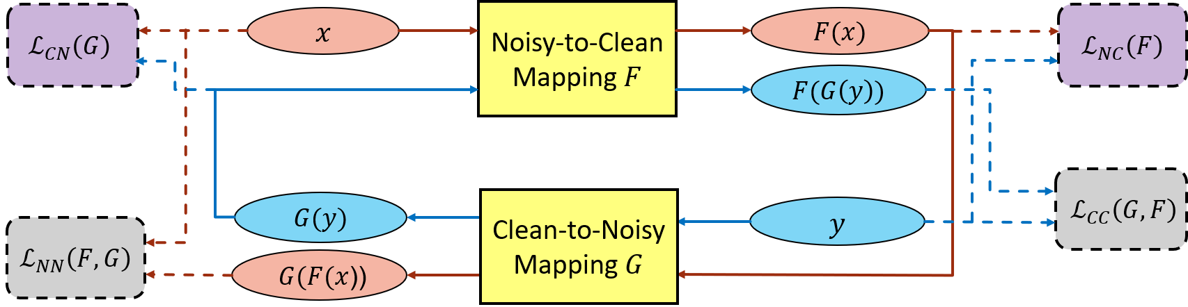
Figure 1: The architecture of CSE. Forward and backward cycles are shown in red and blue lines respectively. Noisy and clean training features $X$ and $Y$ are parallel to each other.

With feature mapping approach for speech enhancement, we are given a sequence of noisy speech features $X=\{x_{1},\ldots,x_{T}\}$ and a sequence of clean speech features $Y=\{y_{1},\ldots,y_{T}\}$ as the training data. $X$ and $Y$ are parallel to each other, i.e., each pair of $x_{i}$ and $y_{i}$ is frame-by-frame synchronized. The goal of speech enhancement is to learn a non-linear mapping network $F$ that transforms $X$ to a sequence of enhanced features $\hat{Y}=\{\hat{y}_{1},\ldots,\hat{y}_{T}\},\hat{y_{i}}=F(x_{i}),i=1,\ldots,T$ such that the distribution of $\hat{Y}$ is as close to $Y$ as possible. To achieve that, we minimize the noisy-to-clean feature-mapping loss $\mathcal{L}_{NC}(F)$, which is commonly defined as the MSE between $\hat{Y}$ and $Y$ as follows.

$$\mathcal{L}_{NC}(F) =\frac{1}{T}\sum_{i=1}^{T}(\hat{y}_{i}-y_{i})^{2}=\frac{1}{T}\sum_{i=1}^{T}\left[F(x_{i})-y_{i}\right]^{2}$$ (1)

In CSE, as shown in Fig. 1, we couple $F$ with a clean-to-noisy (inverse the process of noisy-to-clean) mapping network $G$ which reconstructs the noisy features $X^{r}=\{x^{r}_{1},\ldots,x^{r}_{N}\},x^{r}_{i}=G(\hat{y_{i}})=G(F(x_{i}))$ given $\hat{Y}$. A forward cycle-consistency is enforced to ensure the reconstructed $X^{r}$ to be as close to $X$ as possible and therefore, the noisy reconstruction loss $\mathcal{L}_{NN}(F)$, defined as the MSE between $X^{r}$ and $X$, should be minimized as follows:

$$\mathclap{\mathcal{L}_{NN}(F,G)=\frac{1}{T}\sum_{i=1}^{T}(x_{i}-x^{r}_{i})^{2}=\frac{1}{T}\sum_{i=1}^{T}\left[x_{i}-G(F(x_{i}))\right]^{2}}$$ (2)

The consecutive mappings $F:X\rightarrow\hat{Y}$ followed by $G:\hat{Y}\rightarrow X^{r}$ forms the forward cycle of CSE.

To enhance the generalization of $F$ and $G$, we further introduce a backward cycle of mappings in the opposite direction with the same networks. Specifically, we first map $Y$ to the noised features $\hat{X}=\{\hat{x}_{1},\ldots,\hat{x}_{T}\},\hat{x}_{i}=G(y_{i})$ and minimize the clean-to-noisy feature-mapping loss $\mathcal{L}_{CN}(G)$,

$$\mathcal{L}_{CN}(G) =\frac{1}{T}\sum_{i=1}^{T}(x_{i}-\hat{x}_{i})^{2}=\frac{1}{T}\sum_{i=1}^{T}\left[x_{i}-G(y_{i})\right]^{2}$$ (3)

and then reconstruct the clean features $Y^{r}=\{y^{r}_{1},\ldots,y^{r}_{N}\},y^{r}_{i}=F(\hat{x_{i}})=F(G(y_{i}))$ from $\hat{X}$ and minimize the clean reconstruction loss $\mathcal{L}_{CC}(G,F)$ to enforce the backward cycle-consistency as follows.

$$\mathclap{\mathcal{L}_{CC}(G,F)=\frac{1}{T}\sum_{i=1}^{T}(y_{i}-y^{r}_{i})^{2}=\frac{1}{T}\sum_{i=1}^{T}\left[y_{i}-F(G(y_{i}))\right]^{2}}$$ (4)

In CSE, $F$ and $G$ are jointly trained to minimize the total loss $\mathcal{L}_{CSE}(F,G)$, i.e., the weighted sum of the primary loss $\mathcal{L}_{NC}(F)$ and the secondary losses $\mathcal{L}_{CN}(G)$, $\mathcal{L}_{NN}(F,G)$, $\mathcal{L}_{CC}(G,F)$ in the forward and backward cycles as follows.

$$\mathcal{L}_{\text{CSE}}(F,G)=\mathcal{L}_{NC}(F)+\lambda_{1}\mathcal{L}_{NN}(F,G)$$

$$\quad\quad\quad\quad\quad\quad+\lambda_{2}\mathcal{L}_{CN}(G)+\lambda_{3}\mathcal{L}_{CC}(G,F)$$ (5)

$$(\hat{F},\hat{G})=\min_{F,G}\mathcal{L}_{\text{CSE}}(F,G)$$ (6)

where $\lambda_{1}$, $\lambda_{2}$, $\lambda_{3}$ controls the trade-off among the primary $\mathcal{L}_{NC}(F)$ and the other auxiliary losses. During testing, only $F$ is used to generate the enhanced features given the noisy test features. In Section 4, we will show that both the forward and backward consistencies play important roles in improving speech enhancement performance.

3 Adversarial Cycle-Consistent Speech Enhancement

To make use of the large amount of unparallel noisy and clean data that is much more easily accessible in real scenario, we replace the feature-mapping loss in CSE with adversarial learning loss to propose ACSE.

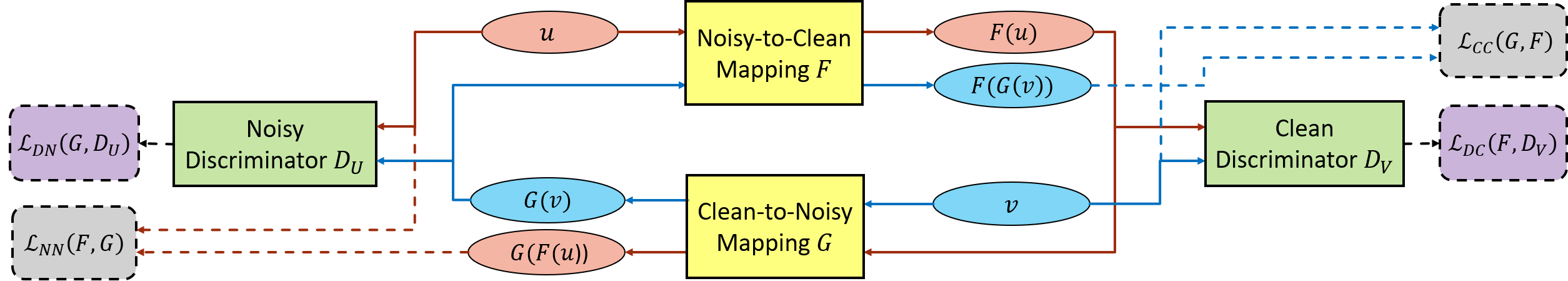
Figure 2: The architecture of ACSE. Forward and backward cycles are shown in red and blue lines respectively. Noisy and clean training features $U$ and $V$ are unparalleled. Identity-mapping losses $\mathcal{L}_{IN}(G)$ and $\mathcal{L}_{IC}(F)$ are not shown in this figure.

Assume that we have a sequence of noisy features $U=\{u_{1},\ldots,u_{T_{u}}\}$ and a sequence of clean features $V=\{v_{1},\ldots,v_{T_{v}}\}$. $U$ and $V$ are unparalleled to each other and conform to the distributions $P_{U}(u)$ and $P_{V}(v)$ respectively. The goal of ACSE is to learn a pair of feature-mapping networks $F$ and $G$ defined in Section 2 such that the distributions of the enhanced features $\hat{V}=\{\hat{v}_{1},\ldots,\hat{v}_{T_{u}}\},\hat{v}_{i}=F(u_{i}),i=1,\ldots,T_{u}$ and the noised features $\hat{U}=\{\hat{u}_{1},\ldots,\hat{u}_{T_{v}}\},\hat{u}_{j}=G(v_{j}),j=1,\ldots,T_{v}$ are as close to the distributions of the $V$ and $U$ as possible, i.e. $P_{\hat{U}}(\hat{u})\rightarrow P_{U}(u)$ and $P_{\hat{U}}(\hat{u})\rightarrow P_{U}(u)$.

To achieve this goal, we introduce two discriminators $D_{U}$ and $D_{V}$ as shown in Fig. 2: $D_{U}$ takes the $\hat{U}$ and $U$ as the input and outputs the posterior probability that an input feature belongs to the noisy set; $D_{V}$ takes the $\hat{V}$ and $V$ as the input and output the posterior probability that an input feature belongs to the clean set, i.e.,

$$D_{U}(u_{i})=P(u_{i}\in\mathbb{N}),\quad 1-D_{U}(\hat{u}_{j})=P(\hat{u}_{j}\in\mathbb{A})$$ (7)

$$D_{V}(v_{j})=P(v_{j}\in\mathbb{C}),\quad 1-D_{V}(\hat{v}_{i})=P(\hat{v}_{i}\in\mathbb{E})$$ (8)

where $\mathbb{C}$, $\mathbb{N}$, $\mathbb{E}$ and $\mathbb{A}$ denotes the sets of clean, noisy, enhanced and noised features respectively. The noisy and clean discrimination losses $\mathcal{L}_{DN}(G,D_{U})$ and $\mathcal{L}_{DC}(F,D_{V})$ for the $D_{U}$ and $D_{V}$ are formulated below using cross-entropy:

$$\mathcal{L}_{DN}(G,D_{U})=\frac{1}{T_{u}}\sum_{i=1}^{T_{u}}\log P(u_{i}\in\mathbb{N})+\frac{1}{T_{v}}\sum_{j=1}^{T_{v}}\log P(\hat{u}_{j}\in\mathbb{A})$$

$$=\frac{1}{T_{u}}\sum_{i=1}^{T_{u}}\log D_{U}(u_{i})+\frac{1}{T_{v}}\sum_{j=1}^{T_{v}}\log\left[1-D_{U}(G(v_{j}))\right]$$ (9)

$$\mathcal{L}_{DC}(F,D_{V})=\frac{1}{T_{v}}\sum_{j=1}^{T_{v}}\log P(v_{j}\in\mathbb{C})+\frac{1}{T_{u}}\sum_{i=1}^{T_{u}}\log P(\hat{v}_{i}\in\mathbb{E})$$

$$=\frac{1}{T_{v}}\sum_{j=1}^{T_{v}}\log D_{V}(v_{j})+\frac{1}{T_{u}}\sum_{i=1}^{T_{u}}\log\left[1-D_{V}(F(u_{i}))\right]$$ (10)

We perform adversarial training of $F$, $G$, $D_{U}$ and $D_{V}$, i.e, we minimize $\mathcal{L}_{DN}(G,D_{U})$ and $\mathcal{L}_{DC}(F,D_{V})$ with respect to $D_{U}$ and $D_{V}$ respectively and simultaneously we maximize them with respect to $F$ and $G$ respectively as follows. This procedure will eventually reach a point where the $F$ and $G$ can generate very confusable $\hat{V}$ and $\hat{U}$ such that $D_{V}$ and $D_{U}$ cannot distinguish them from the V and U.

However, with only the adversarial training, $F$ can map each noisy feature $u_{i}$ to any random permutation of the enhanced features and there is no guarantee that the enhanced feature $\hat{v}_{i}$ is exactly paired with $u_{i}$. To restrict the mapping space of $F$ and $G$, cycle-consistency is enforced by minimizing the noisy and clean reconstruction losses $\mathcal{L}_{NN}(F,G)$ and $\mathcal{L}_{CC}(G,F)$ of $U$ and $V$ as in Section 2.

$$\mathcal{L}_{NN}(F,G)=\frac{1}{T_{u}}\sum_{i=1}^{T_{u}}\left[u_{i}-G(F(u_{i}))\right]^{2}$$ (11)

$$\mathcal{L}_{CC}(G,F)=\frac{1}{T_{v}}\sum_{j=1}^{T_{v}}\left[v_{j}-F(G(v_{j}))\right]^{2}$$ (12)

In addition, we regularize $F$ and $G$ to be close to identity mappings by minimizing the noisy and clean identity-mapping losses below as in [18]:

$$\mathcal{L}_{IN}(G)=\frac{1}{T_{u}}\sum_{i=1}^{T_{u}}\left[u_{i}-G(u_{i})\right]^{2}$$ (13)

$$\mathcal{L}_{IC}(F)=\frac{1}{T_{v}}\sum_{j=1}^{T_{v}}\left[v_{j}-F(v_{j})\right]^{2}$$ (14)

In ACSE, $F$, $G$, $D_{U}$ and $D_{V}$ are jointly trained to optimize the total loss $\mathcal{L}_{\text{ACSE}}$, i.e., the weighted sum of two discrimination losses, two reconstructions losses and two identity-mapping losses through adversarial multi-task learning as follows.

$$\mathcal{L}_{\text{ACSE}}(F,G,D_{V},D_{G})=\left[\mathcal{L}_{NN}(F,G)+\alpha_{1}\mathcal{L}_{CC}(G,F)\right.$$

$$\left.\quad\quad\quad\quad\quad\quad-\alpha_{2}\mathcal{L}_{DN}(G,D_{U})-\alpha_{3}\mathcal{L}_{DC}(F,D_{V})\right.$$

$$\left.\quad\quad\quad\quad\quad\quad+\alpha_{4}\mathcal{L}_{IN}(G)+\alpha_{5}\mathcal{L}_{IC}(F)\right]$$ (15)

$$(\hat{F},\hat{G},\hat{D}_{U},\hat{D}_{V})=\max_{D_{U},D_{V}}\min_{F,G}\mathcal{L}_{\text{ACSE}}(F,G,D_{U},D_{V})$$ (16)

where $\alpha_{1}$, $\alpha_{2}$, $\alpha_{3}$, $\alpha_{4}$ and $\alpha_{5}$ control the trade-off among the primary $\mathcal{L}_{NN}(F,G)$ and the other secondary losses and $\hat{F},\hat{G},\hat{D}_{U},\hat{D}_{V}$ are optimized network parameters. For easy implementation, GRL [37] is introduced and the parameters are optimized using standard stochastic gradient descent. During testing, only the noisy-to-clean mapping network $F$ is used to generate enhanced features given the test noisy features.

4 Experiments

The CHiME-3 dataset [43] incorporates Wall Street Journal (WSJ) corpus sentences spoken in challenging noisy environments, recorded using a 6-channel tablet. We train the noisy-to-clean feature-mapping network $F$ with 9137 clean and 9137 noisy training utterances in CHiME-3 using different methods. The real far-field noisy speech from the 5th microphone channel in CHiME-3 development data set is used for testing. We pre-train a clean DNN acoustic model as in Section 3.2 of [31] using 9137 clean training utterances in CHiME-3 to evaluate the ASR word error rate (WER) performance of the test features enhanced by $F$. The acoustic model is further re-trained with enhanced feature for better WERs. A standard WSJ 5K word 3-gram language model is used for decoding.

4.1 Cycle-Consistent Speech Enhancement

Test Data	BUS	CAF	PED	STR	Avg.	RWERR
No Enhancement	36.25	31.78	22.76	27.18	29.44	0.00
Feature Mapping (baseline)	31.35	28.64	19.80	23.61	25.81	12.33
CSE with Forward Cycle	31.54	27.67	18.62	23.23	25.23	14.30
CSE with Forward and Backward Cycles	30.74	24.87	18.16	21.16	23.67	19.60

Table 1: The ASR WER (%) performance of real noisy test data in CHiME-3 enhanced by different methods evaluated on a clean DNN acoustic model are shown in Columns 2-5. Relative WER reductions (%) (RWERRs) are shown in Column 6.

We use parallel data consisting of 9137 pairs of noisy and clean utterances to train $F$ and clean-to-noisy mapping network $G$. The 29-dimensional log Mel filterbank (LFB) features are extracted for the training data. For the noisy data, LFB features are appended with 1st and 2nd order delta features to form 87-dimensional vectors. $F$ and $G$ are both LSTM-RNNs with 2 hidden layers and 512 units for each hidden layer. A 256-dimensional projection layer is inserted on top of each hidden layer to reduce the number of parameters. $F$ has 87 input units and 29 output units while $G$ has 29 input units and 87 output units. The features are globally mean and variance normalized before fed into $F$ and $G$.

We first train $F$ to minimize $\mathcal{L}_{NC}$ in Eq. 1 as the feature mapping baseline. As shown in Table 1, feature mapping method achieves 25.81% WER when evaluated on the clean acoustic model in [36]. Further, we train $G$ to minimize $\mathcal{L}_{CN}$ in Eq. 3 and couple it with $F$. $F$ and $G$ are jointly trained to minimize $\mathcal{L}_{NC}$, $\mathcal{L}_{CN}$ and $\mathcal{L}_{NC}$ in Eq. (2) to ensure the forward cycle-consistency. WER reduces to 25.23% and achieves 14.30% and 2.25% relative gains over the noisy features and feature mapping baseline respectively.

Finally, the backward cycle-consistency is enforced together with the forward one and $F$ and $G$ are jointly re-trained to minimize the total loss $\mathcal{L}_{\text{CSE}}$ as in Eq. (6). WER further decreases to 23.67% which is 19.60% and 8.29% relative improvements over noisy features and baseline feature mapping. $\lambda_{1}$, $\lambda_{2}$ and $\lambda_{3}$ are set at $0.6$, $0.4$ and $1.4$ respectively and the learning rate is $2\times 10^{-7}$ with a momentum of 0.5 in the experiments. The backward cycle-consistency proves to be effective.

4.2 Adversarial Cycle-Consistent Speech Enhancement

We randomize the 9137 noisy and 9137 clean utterances respectively and use the unparallel data to train $F$ and $G$. The same LFB features are extracted for the training data as in Section 4.1. $F$ and $G$ share the same LSTM architectures as in Section 4.1. The discriminators $D_{U}$ and $D_{V}$ are both feedforward DNNs with 2 hidden layers, 512 units in each hidden layer and 1 unit in the output layer. $D_{U}$ and $D_{V}$ have 87 and 29 input units, respectively.

As the initialization, we first train $F$ with 87 and 29 dimensional noisy features as the input and target respectively and train $G$ with 29 and 87 dimensional clean features as the input and target respectively. Then $F$, $G$, $D_{V}$ and $D_{U}$ are jointly trained to optimize $\mathcal{L}_{\text{ACSE}}$ as in Eq. (16). $\alpha_{1}$, $\alpha_{2}$, $\alpha_{3}$, $\alpha_{4}$ and $\alpha_{5}$ are set at $1.0$, $8.0$, $8.0$, $0.5$ and $0.5$ respectively and the learning rate is $2\times 10^{-7}$ with a momentum of 0.5 in the experiments. As shown in Table 2, ACSE enhanced features achieves 27.47% WER when evaluated on the clean DNN acoustic model, which is 6.69% relative gain over the noisy features.

Test	BUS	CAF	PED	STR	Avg.
Noisy	36.25	31.78	22.76	27.18	29.44
ACSE	33.94	29.87	20.72	25.53	27.47

Table 2: The ASR WER (%) performance of real noisy and ACSE enhanced test data in CHiME-3 evaluated on a clean DNN acoustic model.

4.3 Acoustic Model Re-Training

To improve the ASR performance, we enhance the 9137 noisy utterances in CHiME-3 with ACSE and re-train the clean DNN-HMM acoustic model in [31]. We use the same senone-level forced alignments as the clean model for re-training. The re-trained DNNs are evaluated using noisy and ACSE enhanced test data respectively. As shown in Table 3, ACSE achieves 18.20% WER, which is 38.18% and 5.11% relatively improved over the clean and noisy models.

Train	Test	BUS	CAF	PED	STR	Avg.
Clean	Noisy	36.25	31.78	22.76	27.18	29.44
Noisy	Noisy	25.38	18.17	14.54	18.38	19.18
ACSE	ACSE	24.82	16.97	13.78	17.40	18.20

Table 3: The ASR WER (%) performance of DNN acoustic models re-trained with noisy and ACSE enhanced training data in CHiME-3.

5 Conclusions

In this paper, we proposed CSE to transform noisy speech features to clean ones by using parallel noisy and clean training data. A pair of noisy-to-clean and clean-to-noisy feature-mapping networks $F$ and $G$ are trained to minimize the bidirectional feature-mapping losses and the reconstruction losses which encourage the consecutive feature mappings $F$ and $G$ to reconstruct the original input features with minimized errors. Further we propose ACSE to learn $F$ and $G$ from unparalleled noisy and clean training data by performing adversarial training of $F$, $G$ and two discriminator networks that distinguish the reconstructed clean and noisy features from the real ones. The discrimination losses are jointly optimized with the reconstruction losses through adversarial multi-task learning.

We perform ASR experiments with features enhanced by the proposed methods on CHiME-3 dataset. CSE achieves 19.60% and 8.29% relative WER improvements over the noisy features and feature-mapping baseline when evaluated on a clean DNN acoustic model. Backward cycle-consistency provides substantial improvement on top of forward cycle-consistency alone. When parallel data is not available, ACSE achieves 6.69% relative WER improvement over the noisy features. After re-training the acoustic model, CSE enhanced features achieve 5.11% relative gain over the noisy features.

In the future, we will perform CSE on large datasets to verify its scalability and evaluate its performance using other metrics such as signal-to-noise ratio to justify its effectiveness in other applications. As shown in [44], teacher-student (T/S) learning [45] is better for robust model adaptation without transcription. We are now working on the combination of CSE with T/S learning to further improve the ASR performance.

References

- [1] P. C. Loizou, Speech enhancement: theory and practice. CRC press, 2013.
- [2] G. Hinton, L. Deng, D. Yu et al., “Deep neural networks for acoustic modeling in speech recognition: The shared views of four research groups,” IEEE Signal Processing Magazine, vol. 29, no. 6, pp. 82–97, 2012.
- [3] N. Jaitly, P. Nguyen, A. Senior, and V. Vanhoucke, “Application of pretrained deep neural networks to large vocabulary speech recognition,” in Proc. Interspeech, 2012.
- [4] T. Sainath, B. Kingsbury, B. Ramabhadran et al., “Making deep belief networks effective for large vocabulary continuous speech recognition,” in Proc. ASRU, 2011, pp. 30–35.
- [5] L. Deng, J. Li, J.-T. Huang et al., “Recent advances in deep learning for speech research at Microsoft,” in ICASSP. IEEE, 2013.
- [6] D. Yu and J. Li, “Recent progresses in deep learning based acoustic models,” IEEE/CAA Journal of Automatica Sinica, vol. 4, no. 3, pp. 396–409, 2017.
- [7] J. Li, L. Deng, Y. Gong, and R. Haeb-Umbach, “An overview of noise-robust automatic speech recognition,” IEEEACMTransASLP, vol. 22, no. 4, pp. 745–777, April 2014.
- [8] J. Li, L. Deng, R. Haeb-Umbach, and Y. Gong, Robust Automatic Speech Recognition: A Bridge to Practical Applications. Academic Press, 2015.
- [9] A. Narayanan and D. Wang, “Ideal ratio mask estimation using deep neural networks for robust speech recognition,” in Proc. ICASSP. IEEE, 2013, pp. 7092–7096.
- [10] Y. Wang, A. Narayanan, and D. Wang, “On training targets for supervised speech separation,” IEEE/ACM Transactions on Audio, Speech, and Language Processing, vol. 22, no. 12, pp. 1849–1858, 2014.
- [11] F. Weninger, H. Erdogan, S. Watanabe et al., “Speech enhancement with lstm recurrent neural networks and its application to noise-robust asr,” in International Conference on Latent Variable Analysis and Signal Separation, 2015.
- [12] Y. Xu, J. Du, L. R. Dai, and C. H. Lee, “A regression approach to speech enhancement based on deep neural networks,” IEEE/ACM Transactions on Audio, Speech, and Language Processing, vol. 23, no. 1, pp. 7–19, 2015.
- [13] X. Lu, Y. Tsao, S. Matsuda, and C. Hori, “Speech enhancement based on deep denoising autoencoder.” in Interspeech, 2013, pp. 436–440.
- [14] A. L. Maas, Q. V. Le, T. M. O’Neil, O. Vinyals, P. Nguyen, and A. Y. Ng, “Recurrent neural networks for noise reduction in robust asr,” in Proc. INTERSPEECH, 2012.
- [15] X. Feng, Y. Zhang, and J. Glass, “Speech feature denoising and dereverberation via deep autoencoders for noisy reverberant speech recognition,” in Proc. ICASSP. IEEE, 2014.
- [16] F. Weninger, F. Eyben, and B. Schuller, “Single-channel speech separation with memory-enhanced recurrent neural networks,” in Proc. ICASSP. IEEE, 2014, pp. 3709–3713.
- [17] Z. Chen, Y. Huang, J. Li, and Y. Gong, “Improving mask learning based speech enhancement system with restoration layers and residual connection,” in Proc. Interspeech, 2017.
- [18] J.-Y. Zhu, T. Park, P. Isola, and A. A. Efros, “Unpaired image-to-image translation using cycle-consistent adversarial networkss,” in Proc. ICCV, 2017.
- [19] I. Goodfellow, J. Pouget-Abadie, and et al., “Generative adversarial nets,” in NIPS, 2014.
- [20] A. Radford, L. Metz, and S. Chintala, “Unsupervised representation learning with deep convolutional generative adversarial networks,” CoRR, vol. abs/1511.06434, 2015.
- [21] E. Denton, S. Chintala, A. Szlam, and R. Fergus, “Deep generative image models using a laplacian pyramid of adversarial networks,” in Proc. NIPS, ser. NIPS’15, 2015, pp. 1486–1494.
- [22] P. Isola, J.-Y. Zhu, T. Zhou, and A. A. Efros, “Image-to-image translation with conditional adversarial networks,” CVPR, 2017.
- [23] X. Chen, X. Chen, Y. Duan, Houthooft, and et al., “Infogan: Interpretable representation learning by information maximizing generative adversarial nets,” in Proc. NIPS, 2016.
- [24] S. Pascual, A. Bonafonte, and J. Serrà, “Segan: Speech enhancement generative adversarial network,” in INTERSPEECH, 2017.
- [25] C. Donahue, B. Li, and R. Prabhavalkar, “Exploring speech enhancement with generative adversarial networks for robust speech recognition,” arXiv preprint arXiv:1711.05747, 2017.
- [26] M. Mimura, S. Sakai, and T. Kawahara, “Cross-domain speech recognition using nonparallel corpora with cycle-consistent adversarial networks,” in Proc. ASRU, 2017, pp. 134–140.
- [27] Z. Meng, J. Li, Y. Gong, and B.-H. F. Juang, “Adversarial feature-mapping for speech enhancement,” in Proc. Interspeech, 2018.
- [28] T. Kaneko and H. Kameoka, “Parallel-data-free voice conversion using cycle-consistent adversarial networks,” arXiv preprint arXiv:1711.11293, 2017.
- [29] C.-C. Hsu, H.-T. Hwang, Y.-C. Wu, Y. Tsao, and H.-M. Wang, “Voice conversion from unaligned corpora using variational autoencoding wasserstein generative adversarial networks,” arXiv preprint arXiv:1704.00849, 2017.
- [30] S. Sun, B. Zhang, L. Xie et al., “An unsupervised deep domain adaptation approach for robust speech recognition,” Neurocomputing, 2017.
- [31] Z. Meng, Z. Chen, V. Mazalov, J. Li, and Y. Gong, “Unsupervised adaptation with domain separation networks for robust speech recognition,” in Proceeding of ASRU, Dec 2017.
- [32] Z. Meng, J. Li, Y. Gong, and B.-H. F. Juang, “Adversarial teacher-student learning for unsupervised domain adaptation,” in Proc.ICASSP. IEEE, 2018.
- [33] Y. Shinohara, “Adversarial multi-task learning of deep neural networks for robust speech recognition.” in Proc. Interspeech, 2016, pp. 2369–2372.
- [34] S. Sun, B. Zhang, L. Xie et al., “An unsupervised deep domain adaptation approach for robust speech recognition,” Neurocomputing, 2017.
- [35] G. Saon, G. Kurata, T. Sercu et al., “English conversational telephone speech recognition by humans and machines,” Proc. Interspeech, 2017.
- [36] Z. Meng, J. Li, Z. Chen et al., “Speaker-invariant training via adversarial learning,” in Proc. ICASSP, 2018.
- [37] Y. Ganin and V. Lempitsky, “Unsupervised domain adaptation by backpropagation,” in Proc. NIPS, ser. Proceedings of Machine Learning Research, F. Bach and D. Blei, Eds., vol. 37. Lille, France: PMLR, 07–09 Jul 2015, pp. 1180–1189.
- [38] M. Arjovsky, S. Chintala, and L. Bottou, “Wasserstein gan,” arXiv preprint arXiv:1701.07875, 2017.
- [39] I. Gulrajani, F. Ahmed, M. Arjovsky, V. Dumoulin, and A. C. Courville, “Improved training of wasserstein gans,” in Proc. NIPS, 2017, pp. 5769–5779.
- [40] H. Sak, A. Senior, and F. Beaufays, “Long short-term memory recurrent neural network architectures for large scale acoustic modeling,” in Interspeech, 2014.
- [41] Z. Meng, S. Watanabe, J. R. Hershey, and H. Erdogan, “Deep long short-term memory adaptive beamforming networks for multichannel robust speech recognition,” in ICASSP, 2017.
- [42] H. Erdogan, T. Hayashi, J. R. Hershey et al., “Multi-channel speech recognition: Lstms all the way through,” in CHiME-4 workshop, 2016, pp. 1–4.
- [43] J. Barker, R. Marxer, E. Vincent, and S. Watanabe, “The third chime speech separation and recognition challenge: Dataset, task and baselines,” in Proc. ASRU, 2015, pp. 504–511.
- [44] J. Li, M. L. Seltzer, X. Wang et al., “Large-scale domain adaptation via teacher-student learning,” in Proc. Interspeech, 2017.
- [45] J. Li, R. Zhao, J.-T. Huang, and Y. Gong, “Learning small-size DNN with output-distribution-based criteria.” in Proc. Interspeech, 2014, pp. 1910–1914.