Adversarial Feature-Mapping for Speech Enhancement

Abstract

Feature-mapping with deep neural networks is commonly used for single-channel speech enhancement, in which a feature-mapping network directly transforms the noisy features to the corresponding enhanced ones and is trained to minimize the mean square errors between the enhanced and clean features. In this paper, we propose an adversarial feature-mapping (AFM) method for speech enhancement which advances the feature-mapping approach with adversarial learning. An additional discriminator network is introduced to distinguish the enhanced features from the real clean ones. The two networks are jointly optimized to minimize the feature-mapping loss and simultaneously mini-maximize the discrimination loss. The distribution of the enhanced features is further pushed towards that of the clean features through this adversarial multi-task training. To achieve better performance on ASR task, senone-aware (SA) AFM is further proposed in which an acoustic model network is jointly trained with the feature-mapping and discriminator networks to optimize the senone classification loss in addition to the AFM losses. Evaluated on the CHiME-3 dataset, the proposed AFM achieves 16.95% and 5.27% relative word error rate (WER) improvements over the real noisy data and the feature-mapping baseline respectively and the SA-AFM achieves 9.85% relative WER improvement over the multi-conditional acoustic model.

Index Terms: speech enhancement, paralleled data, adversarial learning, speech recognition

1 Introduction

Single-channel speech enhancement aims at attenuating the noise component of noisy speech to increase the intelligibility and perceived quality of the speech component [1]. It is commonly used to improve the quality of mobile speech communication in noisy environments and enhance the speech signal before amplification in hearing aids and cochlear implants. More importantly, speech enhancement is widely applied as a front-end pre-processing stage to improve the performance of automatic speech recognition (ASR) [2, 3, 4, 5, 6] and speaker recognition under noisy conditions [7, 8].

With the advance of deep learning, deep neural network (DNN) based approaches have achieved great success in single-channel speech enhancement. The mask learning approach [9, 10, 11] is proposed to estimate the ideal ratio mask or ideal binary mask based on noisy input features using a DNN. The mask is used to filter out the noise from the noisy speech and recover the clean speech. However, it has the presumption that the scale of the masked signal is the same as the clean target and the noise is strictly additive and removable by the masking procedure which is generally not true for real recorded stereo data. To deal with this problem, the feature-mapping approach [12, 13, 14, 15, 16, 17] is proposed to train a feature-mapping network that directly transforms the noisy features to enhanced ones. The feature-mapping network serves as a non-linear regression function trained to minimize the feature-mapping loss, i.e., the mean square error (MSE) between the enhanced features and the paralleled clean ones. The application of MSE estimator is based on the homoscedasticity and no auto-correlation assumption of the noise, i.e., the noise needs to have the same variance for each noisy feature and the noise needs to be uncorrelated between different noisy features [18]. This assumption is in general violated for real speech signal (a kind of time series data) under non-stationary unknown noise.

Recently, adversarial training [19] has become a hot topic in deep learning with its great success in estimating generative models. It was first applied to image generation [20, 21], image-to-image translation [22, 23] and representation learning [24]. In speech area, it has been applied to speech enhancement [25, 26, 27, 28], voice conversion [29, 30], acoustic model adaptation [31, 32, 33], noise-robust [34, 35] and speaker-invariant [36, 37] ASR using gradient reversal layer (GRL) [38]. In these works, adversarial training is used to learn a feature or an intermediate representation in DNN that is invariant to the shift among different domains (e.g., environments, speakers, image styles, etc.). In other words, a generator network is trained to map data from different domains to the features with similar distributions via adversarial learning.

Inspired by this, we advance the feature-mapping approach with adversarial learning to further diminish the discrepancy between the distributions of the clean features and the enhanced features generated by the feature-mapping network given non-stationary and auto-correlated noise at the input. We call this method adversarial feature-mapping (AFM) for speech enhancement. In AFM, an additional discriminator network is introduced to distinguish the enhanced features from the real clean ones. The feature-mapping network and the discriminator network are jointly trained to minimize the feature-mapping loss and simultaneously mini-maximize the discrimination loss with adversarial multi-task learning. With AFM, the feature-mapping network can generate pseudo-clean features that the discriminator can hardly tell whether they are real clean features or not. To achieve better performance on ASR task, senone-aware adversarial feature-mapping (SA-AFM) is proposed in which an acoustic model network is introduced and is jointly trained with the feature-mapping and discriminator networks to optimize the senone classification loss in addition to the feature-mapping and discrimination losses.

Note that AFM is different from [26] in that: (1) In AFM, the inputs to the discriminator are enhanced and clean features while in [26] the inputs to the discriminator are the concatenation of enhanced and noisy features and the concatenation of clean and noisy features. (2) The primary task of AFM is feature-mapping, i.e., to minimize the $L_{2}$ distance (MSE) between enhanced and clean features and it is advanced with adversarial learning to further reduce the discrepancy between the distributions of the enhanced and clean features while in [26] the primary task is to generate enhanced features that are similar to clean features with generative adversarial network (GAN) and it is regularized with the minimization of $L_{1}$ distance between noisy and enhanced features. (3) AFM performs adversarial multi-task training using GRL method as in [38] while [26] conducts conditional GAN iterative optimization as in [19]. (4) In this paper, AFM uses long short-term memory (LSTM)-recurrent neural networks (RNNs) [39, 40, 41] to generate the enhanced features and a feed-forward DNN as the discriminator while [26] uses convolutional neural networks for both.

We perform ASR experiments with features enhanced by AFM on CHiME-3 dataset [42]. Evaluated on a clean acoustic model, AFM achieves 16.95% and 5.27% relative word error rate (WER) improvements respectively over the noisy features and feature-mapping baseline and the SA-AFM achieves 9.85% relative WER improvement over the multi-conditional acoustic model.

2 Adversarial Feature-Mapping Speech Enhancement

With feature-mapping approach for speech enhancement, we are given a sequence of noisy speech features $X=\{x_{1},\ldots,x_{T}\}$ and a sequence of clean speech features $Y=\{y_{1},\ldots,y_{T}\}$ as the training data. $X$ and $Y$ are parallel to each other, i.e., each pair of $x_{i}$ and $y_{i}$ is frame-by-frame synchronized. The goal of speech enhancement is to learn a non-linear feature-mapping network $F$ with parameters $\theta_{f}$ that transforms $X$ to a sequence of enhanced features $\hat{Y}=\{\hat{y}_{1},\ldots,\hat{y}_{T}\}$ such that the distribution of $\hat{Y}$ is as close to that of $Y$ as possible:

$$\hat{y_{i}}=F(x_{i}),\quad i=1,\ldots,T$$ (1)

$$P_{\hat{Y}}(\hat{y})\rightarrow P_{Y}(y).$$ (2)

To achieve that, we minimize the noisy-to-clean feature-mapping loss $\mathcal{L}_{F}(\theta_{f})$, which is commonly defined as the MSE between $\hat{Y}$ and $Y$ as follows:

$$\mathcal{L}_{F}(\theta_{f}) =\frac{1}{T}\sum_{i=1}^{T}(\hat{y}_{i}-y_{i})^{2}=\frac{1}{T}\sum_{i=1}^{T}\left[F(x_{i})-y_{i}\right]^{2}.$$ (3)

However, the MSE that feature-mapping approach minimizes is based on the homoscedasticity and no auto-correlation assumption of the noise, i.e., the noise has the same variance for each noisy feature and the noise is uncorrelated between different noisy features. This assumption is in general invalid for real speech signal (time series data) under non-stationary unknown noise. To address this problem, we further advance the feature-mapping network with an additional discriminator network and perform adversarial multi-task training to further reduce the discrepancy between the distribution of enhanced features and the clean ones given non-stationary and auto-correlated noise is at the input.

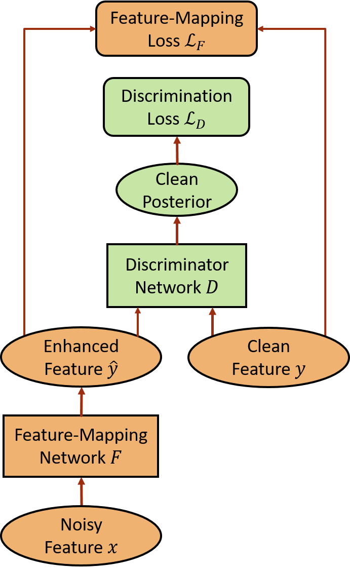
Figure 1: The framework of AFM for speech enhancement.

As shown in Fig. 1, the discriminator network $D$ with parameters $\theta_{d}$ takes enhanced features $\hat{Y}$ and clean features $Y$ as the input and outputs the posterior probability that an input feature belongs to the clean set, i.e.,

$$P(y_{i}\in\mathbb{C}) =D(y_{i})$$ (4)

$$P(\hat{y}_{i}\in\mathbb{E}) =1-D(\hat{y}_{i})$$ (5)

where $\mathbb{C}$ and $\mathbb{E}$ denote the sets of clean and enhanced features respectively. The discrimination losses $\mathcal{L}_{D}(\theta_{f},\theta_{d})$ for the $D$ is formulated below using cross-entropy:

$$\mathcal{L}_{D}(\theta_{f},\theta_{d})=\frac{1}{T}\sum_{i=1}^{T}\left[\log P(y_{i}\in\mathbb{C})+\log P(\hat{y}_{i}\in\mathbb{E})\right]$$

$$=\frac{1}{T}\sum_{i=1}^{T}\log D(y_{i})+\log\left[1-D(F(x_{i}))\right].$$ (6)

To make the distribution of the enhanced features $\hat{Y}$ similar to that of the clean ones $Y$, we perform adversarial training of $F$ and $D$, i.e, we minimize $\mathcal{L}_{D}(\theta_{f},\theta_{d})$ with respect to $\theta_{d}$ and maximize $\mathcal{L}_{D}(\theta_{f},\theta_{d})$ with respect to $\theta_{f}$. This minimax competition will first increase the generation capability of $F$ and the discrimination capability of $D$ and will eventually converge to the point where the $F$ generates extremely confusing enhanced features that $D$ is unable to distinguish whether it is a clean feature or not.

The total loss of AFM $\mathcal{L}_{AFM}(\theta_{f},\theta_{d})$ is formulated as the weighted sum of the feature-mapping loss and the discrimination loss below:

$$\mathcal{L}_{\text{AFM}}(\theta_{f},\theta_{d})=\mathcal{L}_{F}(\theta_{f})-\lambda\mathcal{L}_{D}(\theta_{f},\theta_{d})$$ (7)

where $\lambda>0$ is the gradient reversal coefficient that controls the trade-off between the feature-mapping loss and the discrimination loss in Eq. (3) and Eq. (6) respectively.

$F$ and $D$ are jointly trained to optimize the total loss through adversarial multi-task learning as follows:

$$\hat{\theta}_{f}=\operatorname*{arg\,min}_{\theta_{f}}\mathcal{L}_{\text{AFM}}(\theta_{f},\hat{\theta}_{d})$$ (8)

$$\hat{\theta}_{d}=\operatorname*{arg\,max}_{\theta_{d}}\mathcal{L}_{\text{AFM}}(\hat{\theta}_{f},\theta_{d})$$ (9)

where $\hat{\theta}_{f}$ and $\hat{\theta}_{d}$ are optimal parameters for $F$ and $D$ respectively and are updated as follows via back propagation through time (BPTT) with stochastic gradient descent (SGD):

$$\theta_{f}\leftarrow\theta_{f}-\mu\left[\frac{\partial\mathcal{L}_{\text{F}}(\theta_{f})}{\partial\theta_{f}}-\lambda\frac{\partial\mathcal{L}_{\text{D}}(\theta_{f},\theta_{d})}{\partial\theta_{f}}\right]$$ (10)

$$\theta_{d}\leftarrow\theta_{d}-\mu\frac{\partial\mathcal{L}_{\text{D}}(\theta_{f},\theta_{d})}{\partial\theta_{d}}$$ (11)

where $\mu$ is the learning rate.

Note that the negative coefficient $-\lambda$ in Eq. (10) induces reversed gradient that maximizes $\mathcal{L}_{D}(\theta_{f},\theta_{d})$ in Eq. (6) and makes the enhanced features similar to the real clean ones. Without the reversal gradient, SGD would make the enhanced features different from the clean ones in order to minimize Eq. (6). For easy implementation, gradient reversal layer is introduced in [38], which acts as an identity transform in the forward propagation and multiplies the gradient by $-\lambda$ during the backward propagation. During testing, only the optimized feature-mapping network $F$ is used to generate the enhanced features given the noisy test features.

3 Senone-Aware Adversarial Feature-Mapping Enhancement

For AFM speech enhancement, we only need parallel clean and noisy speech for training and we do not need any information about the content of the speech, i.e., the transcription. With the goal of improving the intelligibility and perceived quality of the speech, AFM can be widely used in a broad range of applications including ASR, mobile communication, hearing aids, cochlear implants, etc. However, for the most important ASR task, AFM does not necessarily lead to the best WER performance because its feature-mapping and discrimination objectives are not directly related to the speech units (i.e., word, phoneme, senone, etc.) classification. In fact, with AFM, some decision boundaries among speech units may be distorted in searching for an optimal separation between speech and noise.

To compensate for this mismatch, we incorporate a DNN acoustic model into the AFM framework and propose the senone-aware adversarial feature-mapping (SA-AFM), in which the acoustic model network $M$, feature-mapping network $F$ and the discriminator network $D$ are trained to jointly optimize the primary task of feature-mapping, secondary task of the third task of clean/enhanced data discrimination and the third task of senone classification in an adversarial fashion. The transcription of the parallel clean and noisy training utterances is required for SA-AFM speech enhancement.

Specifically, as shown in Fig. 2, the acoustic model network $M$ with parameters $\theta_{m}$ takes in the enhanced features $\hat{Y}$ as the input and predicts the senone posteriors $P(q|\hat{y}_{i};\theta_{y}),q\in\mathcal{Q}$ as follows:

$$M(\hat{y}_{i})=P(q|\hat{y}_{i};\theta_{m})，$$ (12)

after the integration with feature-mapping network $F$, we have

$$M(F(x_{i}))=P(q|x_{i};\theta_{f},\theta_{m}).$$ (13)

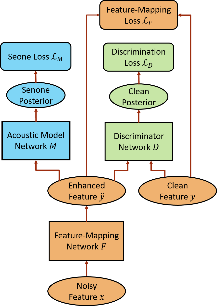
Figure 2: The framework of SA-AFM for speech enhancement.

We want to make the enhanced features $\hat{Y}$ senone-discriminative by minimizing the cross-entropy loss between the predicted senone posteriors and the senone labels as follows:

$$\mathcal{L}_{\text{M}}(\theta_{m},\theta_{f}) =-\frac{1}{T}\sum_{i=1}^{T}\log P(s_{i}|x_{i};\theta_{f},\theta_{m})$$

$$=-\frac{1}{T}\sum_{i=1}^{T}\log M(F(x_{i}))$$ (14)

where $S$ is a sequence of senone labels $S=\{s_{1},\ldots,s_{T}\}$ aligned with the noisy data $X$ and enhanced data $\hat{Y}$.

Simultaneously, we minimize feature-mapping loss $\mathcal{L}_{F}(\theta_{f})$ defined in Eq. (3) with respect to $F$ and perform adversarial training of $F$ and $D$, i.e, we minimize $\mathcal{L}_{D}(\theta_{f},\theta_{d})$ defined in Eq. (6) with respect to $\theta_{d}$ and maximize $\mathcal{L}_{D}(\theta_{f},\theta_{d})$ with respect to $\theta_{f}$, to make the distribution of the enhanced features $\hat{Y}$ similar to that of the clean ones $Y$.

The total loss of SA-AFM $\mathcal{L}_{\text{SA-AFM}}(\theta_{m},\theta_{f},\theta_{d})$ is formulated as the weighted sum of $\mathcal{L}_{F}(\theta_{f})$, $\mathcal{L}_{D}(\theta_{f},\theta_{d})$ and the senone classification loss $\mathcal{L}_{\text{M}}(\theta_{m},\theta_{f})$ as follows:

$$\mathcal{L}_{\text{SA-AFM}}(\theta_{f},\theta_{d},\theta_{m})= \mathcal{L}_{F}(\theta_{f})-\lambda_{1}\mathcal{L}_{D}(\theta_{f},\theta_{d})$$

$$+\lambda_{2}\mathcal{L}_{M}(\theta_{f},\theta_{m})$$ (15)

where $\lambda_{1}>0$ is the gradient reversal coefficient that controls the trade-off between $\mathcal{L}_{F}(\theta_{f})$ and $\mathcal{L}_{D}(\theta_{f},\theta_{d})$, and $\lambda_{2}>0$ is the weight for $\mathcal{L}_{M}(\theta_{f},\theta_{m})$.

$F$, $D$ and $M$ are jointly trained to optimize the total loss through adversarial multi-task learning as follows:

$$(\hat{\theta}_{f},\hat{\theta}_{m})=\operatorname*{arg\,min}_{\theta_{f},\theta_{m}}\mathcal{L}_{\text{SA-AFM}}(\theta_{f},\hat{\theta}_{d},\theta_{m})$$ (16)

$$\hat{\theta}_{d}=\operatorname*{arg\,max}_{\theta_{d}}\mathcal{L}_{\text{SA-AFM}}(\hat{\theta}_{f},\theta_{d},\hat{\theta}_{m})$$ (17)

where $\hat{\theta}_{f}$, $\hat{\theta}_{d}$ and $\hat{\theta}_{m}$ are optimal parameters for $F$, $D$ and $M$ respectively and are updated as follows via BPTT with SGD as in Eq. (10), Eq. (11) and Eq. (18) below:

$$\theta_{m}\leftarrow\theta_{m}-\mu\frac{\partial\mathcal{L}_{\text{M}}(\theta_{f},\theta_{m})}{\partial\theta_{m}}.$$ (18)

During decoding, only the optimized feature-mapping network $F$ and acoustic model network $M$ are used to take in the noisy test features and generate the acoustic scores.

4 Experiments

In the experiments, we train the feature-mapping network $F$ with the parallel clean and noisy training utterances in CHiME-3 dataset [42] using different methods. The real far-field noisy speech from the 5th microphone channel in CHiME-3 development data set is used for testing. We use a pre-trained clean DNN acoustic model to evaluate the ASR WER performance of the test features enhanced by $F$. The standard WSJ 3-gram language model with 5K-word lexicon is used in our experiments.

4.1 Feedforward DNN Acoustic Model

To evaluate the ASR performance of the features enhanced by AFM, we first train a feedforward DNN-hidden Markov model (HMM) acoustic model using 8738 clean training utterances in CHiME-3 with cross-entropy criterion. The 29-dimensional log Mel filterbank (LFB) features together with 1st and 2nd order delta features (totally 87-dimensional) are extracted. Each feature frame is spliced together with 5 left and 5 right context frames to form a 957-dimensional feature. The spliced features are fed as the input of the feed-forward DNN after global mean and variance normalization. The DNN has 7 hidden layers with 2048 hidden units for each layer. The output layer of the DNN has 3012 output units corresponding to 3012 senone labels. Senone-level forced alignment of the clean data is generated using a Gaussian mixture model-HMM system. A WER of 29.44% is achieved when evaluating the clean DNN acoustic model on the test data.

4.2 Adversarial Feature-Mapping Speech Enhancement

We use parallel data consisting of 8738 pairs of noisy and clean utterances in CHiME-3 as the training data. The 29-dimensional LFB features are extracted for the training data. For the noisy data, the 29-dimensional LFB features are appended with 1st and 2nd order delta features to form 87-dimensional feature vectors. $F$ is an LSTM-RNN with 2 hidden layers and 512 units for each hidden layer. A 256-dimensional projection layer is inserted on top of each hidden layer to reduce the number of parameters. $F$ has 87 input units and 29 output units. The features are globally mean and variance normalized before fed into $F$. The discriminator $D$ is a feedforward DNN with 2 hidden layers and 512 units in each hidden layer. $D$ has 29 input units and one output unit.

We first train $F$ with 87-dimensional LFB features as the input and 29-dimensional LFB features as the target to minimize the feature-mapping loss $\mathcal{L}(\theta_{f})$ in Eq. (3). This serves as the feature-mapping baseline. Evaluated on clean DNN acoustic model trained in Section 4.1, the feature-mapping enhanced features achieve 25.81% WER which is 12.33% relative improvement over the noisy features. Then we jointly train $F$ and $D$ to optimize $\mathcal{L}_{\text{AFM}}(\theta_{f},\theta_{d})$ as in Eq. (7) using the same input features and targets. The gradient reversal coefficient $\lambda$ is fixed at $60$ and the learning rate is $5\times 10^{-7}$ with a momentum of $0.5$ in the experiments. As shown in Table 1, AFM enhanced features achieve 24.45% WER which is 16.95 % and 5.27% relative improvements over the noisy features and feature-mapping baseline.

Test Data	BUS	CAF	PED	STR	Avg.
Noisy	36.25	31.78	22.76	27.18	29.44
FM	31.35	28.64	19.80	23.61	25.81
AFM	30.97	26.09	18.40	22.53	24.45

Table 1: The ASR WER (%) performance of real noisy dev set in CHiME-3 enhanced by different methods evaluated on a clean DNN acoustic model. FM represents feature-mapping.

4.3 Senone-Aware Adversarial Feature-Mapping Speech Enhancement

The SA-AFM experiment is conducted on top of the AFM system described in Section 4.2. In addition to the LSTM $F$ and feedforward DNN $D$, we train a multi-conditional LSTM acoustic model $M$ using both the 8738 clean and 8738 noisy training utterances in CHiME-3 dataset. The LSTM $M$ has 4 hidden layers with 1024 units in each layer. A 512-dimensional projection layer is inserted on top each hidden layer to reduce the number of parameters. The output layer has 3012 output units predicting senone posteriors. The senone-level forced alignment of the training data is generated using a GMM-HMM system. As shown in Table 2, the multi-conditional acoustic model achieves 19.28% WER on CHiME-3 simulated dev set.

System	BUS	CAF	PED	STR	Avg.
Multi-Condition	18.44	23.37	16.81	18.50	19.28
SA-FM	18.19	22.29	15.31	18.26	18.51
SA-AFM	17.02	21.01	14.41	17.13	17.38

Table 2: The ASR WER (%) performance of simulated noisy dev set in CHiME-3 by using multi-conditional acoustic model and different enhancement methods.

Then we perform senone-aware feature-mapping (SA-FM) by jointly training $F$ and $M$ to optimize the feature-mapping loss and the senone classification loss in which $M$ takes the enhanced LFB features generated by $F$ as the input to predict the senone posteriors. The SA-FM achieves 18.51% WER on the same testing data. Finally, SA-AFM is performed as described in Section 3 and it achieves 17.38% WER which is 9.85% and 6.10% relative improvements over the multi-conditional acoustic model and SA-FM baseline.

5 Conclusions

In this paper, we advance feature-mapping approach with adversarial learning by proposing AFM method for speech enhancement. In AFM, we have a feature-mapping network $F$ that transforms the noisy speech features to clean ones with parallel noisy and clean training data and a discriminator $D$ that distinguishes the enhanced features from the clean ones. $F$ and $D$ are jointly trained to minimize the feature-mapping loss (i.e., MSE) and simultaneously mini-maximize the discrimination loss. On top of feature-mapping, AFM pushes the distribution of the enhanced features further towards that of the clean features with adversarial multi-task learning.To achieve better performance on ASR task, SA-AFM is further proposed to optimize the senone classification loss in addition to the AFM losses.

We perform ASR experiments with features enhanced by AFM on CHiME-3 dataset. AFM achieves 16.95% and 5.27% relative WER improvements over the noisy features and feature-mapping baseline when evaluated on a clean DNN acoustic model. Furthermore, the proposed SA-AFM achieves 9.85% relative WER improvement over the multi-conditional acoustic model. As we show in [43], teacher-student (T/S) learning [44] is better for robust model adaptation without the need of transcription. We are now working on the combination of AFM with T/S learning to further improve the ASR model performance.

References

- [1] P. C. Loizou, Speech enhancement: theory and practice. CRC press, 2013.
- [2] G. Hinton, L. Deng, D. Yu et al., “Deep neural networks for acoustic modeling in speech recognition: The shared views of four research groups,” IEEE Signal Processing Magazine, vol. 29, no. 6, pp. 82–97, 2012.
- [3] N. Jaitly, P. Nguyen, A. Senior, and V. Vanhoucke, “Application of pretrained deep neural networks to large vocabulary speech recognition,” in Proc. Interspeech, 2012.
- [4] T. Sainath, B. Kingsbury, B. Ramabhadran et al., “Making deep belief networks effective for large vocabulary continuous speech recognition,” in Proc. ASRU, 2011, pp. 30–35.
- [5] L. Deng, J. Li, J.-T. Huang et al., “Recent advances in deep learning for speech research at Microsoft,” in ICASSP. IEEE, 2013.
- [6] D. Yu and J. Li, “Recent progresses in deep learning based acoustic models,” IEEE/CAA Journal of Automatica Sinica, vol. 4, no. 3, pp. 396–409, 2017.
- [7] J. Li, L. Deng, Y. Gong, and R. Haeb-Umbach, “An overview of noise-robust automatic speech recognition,” IEEEACMTransASLP, vol. 22, no. 4, pp. 745–777, April 2014.
- [8] J. Li, L. Deng, R. Haeb-Umbach, and Y. Gong, Robust Automatic Speech Recognition: A Bridge to Practical Applications. Academic Press, 2015.
- [9] A. Narayanan and D. Wang, “Ideal ratio mask estimation using deep neural networks for robust speech recognition,” in ICASSP. IEEE, 2013.
- [10] Y. Wang, A. Narayanan, and D. Wang, “On training targets for supervised speech separation,” IEEE/ACM Transactions on Audio, Speech, and Language Processing, vol. 22, no. 12, pp. 1849–1858, Dec 2014.
- [11] F. Weninger, H. Erdogan, S. Watanabe et al., “Speech enhancement with lstm recurrent neural networks and its application to noise-robust asr,” in International Conference on Latent Variable Analysis and Signal Separation, 2015.
- [12] Y. Xu, J. Du, L. R. Dai, and C. H. Lee, “A regression approach to speech enhancement based on deep neural networks,” IEEE/ACM Transactions on Audio, Speech, and Language Processing, vol. 23, no. 1, pp. 7–19, Jan 2015.
- [13] X. Lu, Y. Tsao, S. Matsuda, and C. Hori, “Speech enhancement based on deep denoising autoencoder.” in Proc. Interspeech, 2013.
- [14] A. L. Maas, Q. V. Le, and et al., “Recurrent neural networks for noise reduction in robust ASR,” in Proc. Interspeech, 2012.
- [15] X. Feng, Y. Zhang, and J. Glass, “Speech feature denoising and dereverberation via deep autoencoders for noisy reverberant speech recognition,” in Proc. ICASSP, 2014, pp. 1759–1763.
- [16] F. Weninger, F. Eyben, and B. Schuller, “Single-channel speech separation with memory-enhanced recurrent neural networks,” in Proc. ICASSP. IEEE, 2014, pp. 3709–3713.
- [17] Z. Chen, Y. Huang, J. Li, and Y. Gong, “Improving mask learning based speech enhancement system with restoration layers and residual connection,” in Proc. Interspeech, 2017.
- [18] D. A. Freedman, Statistical models: theory and practice. cambridge university press, 2009.
- [19] I. Goodfellow, J. Pouget-Abadie, and et al., “Generative adversarial nets,” in NIPS, 2014.
- [20] A. Radford, L. Metz, and S. Chintala, “Unsupervised representation learning with deep convolutional generative adversarial networks,” CoRR, vol. abs/1511.06434, 2015.
- [21] E. Denton, S. Chintala, A. Szlam, and R. Fergus, “Deep generative image models using a laplacian pyramid of adversarial networks,” in Proceedings of the 28th International Conference on Neural Information Processing Systems - Volume 1, ser. NIPS’15. MIT Press, 2015, pp. 1486–1494.
- [22] P. Isola, J.-Y. Zhu, T. Zhou, and A. A. Efros, “Image-to-image translation with conditional adversarial networks,” CVPR, 2017.
- [23] J.-Y. Zhu, T. Park, P. Isola, and A. A. Efros, “Unpaired image-to-image translation using cycle-consistent adversarial networkss,” in ICCV, 2017.
- [24] X. Chen, Y. Duan, and et al., “Infogan: Interpretable representation learning by information maximizing generative adversarial nets,” in NIPS, 2016.
- [25] S. Pascual, A. Bonafonte, and J. Serrà, “Segan: Speech enhancement generative adversarial network,” in Interspeech, 2017.
- [26] C. Donahue, B. Li, and R. Prabhavalkar, “Exploring speech enhancement with generative adversarial networks for robust speech recognition,” arXiv preprint arXiv:1711.05747, 2017.
- [27] M. Mimura, S. Sakai, and T. Kawahara, “Cross-domain speech recognition using nonparallel corpora with cycle-consistent adversarial networks,” in Proc. ASRU, Dec 2017, pp. 134–140.
- [28] Z. Meng, J. Li, Y. Gong, and B.-H. F. Juang, “Cycle-consistent speech enhancement,” in Proc. Interspeech, 2018.
- [29] T. Kaneko and H. Kameoka, “Parallel-data-free voice conversion using cycle-consistent adversarial networks,” arXiv preprint arXiv:1711.11293, 2017.
- [30] C.-C. Hsu, H.-T. Hwang, Y.-C. Wu, Y. Tsao, and H.-M. Wang, “Voice conversion from unaligned corpora using variational autoencoding wasserstein generative adversarial networks,” arXiv preprint arXiv:1704.00849, 2017.
- [31] S. Sun, B. Zhang, L. Xie et al., “An unsupervised deep domain adaptation approach for robust speech recognition,” Neurocomputing.
- [32] Z. Meng, Z. Chen, V. Mazalov, J. Li, and Y. Gong, “Unsupervised adaptation with domain separation networks for robust speech recognition,” in Proceeding of ASRU, Dec 2017.
- [33] Z. Meng, J. Li, Y. Gong, and B.-H. F. Juang, “Adversarial teacher-student learning for unsupervised domain adaptation,” in Proc.ICASSP. IEEE, 2018.
- [34] Y. Shinohara, “Adversarial multi-task learning of deep neural networks for robust speech recognition.” in Interspeech, 2016, pp. 2369–2372.
- [35] D. Serdyuk, K. Audhkhasi, P. Brakel, B. Ramabhadran et al., “Invariant representations for noisy speech recognition,” in NIPS Workshop, 2016.
- [36] G. Saon, G. Kurata, T. Sercu et al., “English conversational telephone speech recognition by humans and machines,” Proc. Interspeech, 2017.
- [37] Z. Meng, J. Li, Z. Chen et al., “Speaker-invariant training via adversarial learning,” in Proc. ICASSP, 2018.
- [38] Y. Ganin and V. Lempitsky, “Unsupervised domain adaptation by backpropagation,” in ICML, 2015.
- [39] H. Sak, A. Senior, and F. Beaufays, “Long short-term memory recurrent neural network architectures for large scale acoustic modeling,” in Interspeech, 2014.
- [40] Z. Meng, S. Watanabe, J. R. Hershey, and H. Erdogan, “Deep long short-term memory adaptive beamforming networks for multichannel robust speech recognition,” in ICASSP, 2017.
- [41] H. Erdogan, T. Hayashi, J. R. Hershey et al., “Multi-channel speech recognition: Lstms all the way through,” in CHiME-4 workshop, 2016, pp. 1–4.
- [42] J. Barker, R. Marxer, E. Vincent, and S. Watanabe, “The third CHiME speech separation and recognition challenge: Dataset, task and baselines,” in Proc. ASRU, 2015, pp. 504–511.
- [43] J. Li, M. L. Seltzer, X. Wang et al., “Large-scale domain adaptation via teacher-student learning,” in Proc. Interspeech, 2017.
- [44] J. Li, R. Zhao, J.-T. Huang, and Y. Gong, “Learning small-size DNN with output-distribution-based criteria.” in Proc. Interspeech, 2014, pp. 1910–1914.