Excitation spectra of exotic nuclei in a self-consistent phonon-coupling model

Abstract

We explore giant resonance spectra and low-lying dipole strength in the Ni and Sn chains from proton rich to very neutron rich isotopes, relevant in astrophysical reaction chains. For the theoretical description we employ the random-phase approximation (RPA) plus many-body effects through a phonon coupling model with optimized selection of phonons. The nuclear force is based on the Skyrme-Hartree-Fock energy functional carried consistently through all steps of modelling. The main effect of phonon coupling is a broadening of the spectral distributions (collisional width). This broadening is particularly dramatic for low-lying dipole strength in very neutron rich nuclei delivering there a qualitative change of the spectra.

I Introduction

For several decades, an extension of the random-phase approximation (RPA) which includes the effects of the quasiparticle-phonon coupling Soloviev (1992); Bertsch et al. (1983); Kamerdzhiev et al. (2004) has been successfully applied in nuclear structure calculations. The coupling to phonons gives rise to a broadening of the RPA states which is called collisional broadening Bertsch et al. (1983) and which adds to the escape width from coupling to single-particle continuum. An other very important effect is the fragmentation of the bound collective states. Due to this effect the low-lying collective $3^{-}$, $5^{-}$ and $2^{+}$ states are shifted to lower energies without increasing the corresponding BE-values Tselyaev et al. (2017). This solved a problem in conventional RPA calculations which usually highly overestimate the BE-values if one tries to reproduce the excitation energies. There exists many different versions of quasiparticle-phonon coupling models. They include the quasiparticle-phonon model Soloviev (1992); Vdovin and Soloviev (1983); Voronov and Soloviev (1983), the core-coupling RPA Dehesa et al. (1977), the particle-vibration coupling model Bertsch et al. (1983); Colò et al. (1994); Colò and Bortignon (2001); Roca-Maza et al. (2017), the two-phonon extended RPA Barbieri and Dickhoff (2003); Dickhoff and Barbieri (2004), and the different versions of the time-blocking approximation (TBA) Tselyaev (1989); Kamerdzhiev et al. (1993, 2004); Tselyaev (2007); Litvinova et al. (2007, 2008); Lyutorovich et al. (2015, 2016); Tselyaev et al. (2016, 2017, 2018) developed within the many-body Green-functions formalism. Here we use the self-consistent version of the TBA developed in a series of our recent papers Lyutorovich et al. (2015, 2016); Tselyaev et al. (2016, 2017, 2018) where we used different approximations to solve the TBA equations within this approach.

Although successful, phonon-coupling models leave some ambiguity concerning the choice of the number of RPA phonons which one includes in the numerical approaches as the energy shift and the fragmentation of the single-particle strength depends on this number. As only a few of the RPA solutions represent collective states and the majority of the solutions are more or less one-particle one-hole ($ph$) states, a too large number of phonons would cause a violation of the Pauli principle and it would introduce a severe problem of double counting. Various measures to confine the selection of coupling phonons to “collective” ones had been considered in the past. We first selected the phonons according to their reduced transition probability only considering states which exhausted a certain fraction of the total transition strength. Here one assumes that the most collective states also couple most strongly to the single-particle ($sp$) states which however, is not so obvious. Recently we introduced a modified method of the TBA which allows the selections of phonons in terms of dimensionless coupling strengths Tselyaev et al. (2017) and for which we have demonstrated that it converges very fast and delivers clear cut criteria. Lately we developed a nonlinear version of our phonon-coupling model, an extended TBA, convergences automatically when enlarging the phonon space Tselyaev et al. (2018). With this extended TBA, we have counter-checked our previously developed cutoff criteria and found them confirmed. As the new, extended TBA is much more computer time consuming we used the previous cutoff criterion in which the relevant phonons (positive frequency: $\omega^{\vphantom{*}}_{n}>0$) are chosen according to Tselyaev et al. (2017)

$$|\,v^{\vphantom{*}}_{n}\,|>v_{\mbox{\scriptsize min}}\;,\;v^{\vphantom{*}}_{n}=\langle\,V\,\rangle^{\vphantom{*}}_{n}/\omega^{\vphantom{*}}_{n}\;,$$ (1a)

where $$\langle\,V\,\rangle^{\vphantom{*}}_{n} |\,{z}^{n}\rangle \omega_{n} v_{n} v_{\mbox{\scriptsize min}}$$ represents the average residual interaction in a given RPA state with the energy . This means that one considers only those phonons whose dimensionless interaction strength is larger than the cutoff value . The mean value of the residual interaction is connected with the energy shift of a given RPA state

$$\langle\,V\,\rangle^{\vphantom{*}}_{n}=|\,\omega^{\vphantom{*}}_{n}|-|\,\omega^{(0)}_{n}|\,.$$ (1b)

where

$$|\,\omega^{(0)}_{n}|=\sum_{ph}\,(\varepsilon^{\vphantom{*}}_{p}-\varepsilon^{\vphantom{*}}_{h})\bigl{(}\,|\,z^{n}_{ph}\,|^{2}+|\,z^{n}_{hp}\,|^{2}\bigr{)}\,.$$ (1c)

is the average single-particle energy of state $n$. Collective states are distinguished by a strong shift in energy. Therefore, this criterion picks preferably collective states as desired. The success depends on choosing a proper values for the cutoff parameter $v_{\mbox{\scriptsize min}}=0.05$. In Ref. Tselyaev et al. (2017) it has been demonstrated that stable results are obtained for the parameter $v_{\mbox{\scriptsize min}}$ in the range 0.01–0.1 in which the numerical results remain nearly unchanged. In the actual calculations we will chose $v_{\mbox{\scriptsize min}}=0.05$.

In the present publication, we apply TBA to two chains of doubly magic nuclei ranging deep into the regime of exotic nuclei relevant for astro-physical reaction chains Arnould et al. (2007). We calculated excitation energies and transition probabilities of bound states as well as dipole strength distributions in the regime of giant resonances for four Ni (^48,56,68,78Ni) isotopes and four Sn (^{100,132,140,176}Sn) isotopes. Both considered isotope chains are unique in the nuclear chart because in all these cases there exists a certain chance to obtain experimental numbers for some of the low-lying collective states and giant resonances. For the more stable members of the chains, experimental values do already exist and will be referred to later on. We expect reliable results as our theoretical model has been successfully tested on several doubly magic nuclei, including ⁵⁶Ni and ¹³²Sn from the present chains.

Furthermore, we have a look at the low-lying electric dipole strength in these nuclei. Although we do not find particularly collective states in this region (in accordance with Reinhard and Nazarewicz (2013a)), we denote it here by the nickname pygmy dipole resonance (PDR) as commonly used in the literature. The structural changes in the PDR region along the isotopes are particularly interesting because our chains span from proton rich isotopes to very neutron rich ones.

We ought to mention that there exist numerous theoretical publications where aspects of our investigation have been addressed. We try to summarize these references restricting ourselves to Ni and Sn isotopes. The question of a possible magic neutron number $N=40$ has been discussed in Refs. Yao et al. (2015); Saxena and Kaushik (2017). This is important in connection with the “magic” nucleus ⁶⁸Ni which we investigate in our paper. For this isotope, several experimental data exist: (I) the PDR Wieland et al. (2009); Wieland and Bracco (2011) and (II) the isoscalar giant monopole resonance (GMR) Vandebrouck et al. (2014). The absense of the low-lying pigmy resonance in the ⁶⁸Ni monopole response function is discussed in Hamamoto and Sagawa (2014).

In many of the papers the giant dipole resonance (GDR) and the low-lying dipole strength have been addressed. In the proton rich ⁴⁸Ni isotope, the PDR has been identified as a vibration of loosely bound protons against the proton-neutron symmetric core. Here two different nuclear structure models have been used Paar et al. (2005). Within a self-consistent quasiparticle RPA the low-lying dipole strength has been calculated Papakonstantinou et al. (2014, 2015a) in a number of Sn isotopes using the Gogny force and in a similar approach also Ni isotopes were investigated Papakonstantinou et al. (2015b). In Ref. Co’ et al. (2013), the PDR was studied in various medium and heavy nuclei with self-consistent RPA models using also the Gogny interaction. Here, a detailed comparison of the PDR and the conventional GDR was given. The E1 strength for fifteen Sn isotopes haven been calculated in self-consistent models including pairing correlations Avdeenkov et al. (2011). The authors also highlighted the astrophysical aspect of their investigation. The energy of the $2^{+}_{1}$ state in ^68,78Ni and other Ni isotopes were calculated in Ref. Hagen et al. (2016) in the framework of the coupled-cluster theory with chiral nucleon-nucleon and three-nucleon interactions. The continuum was taken into account by employing the Berggreen basis which treats bound-, resonant-, and non-resonant scattering states on equal footing. The predicted range for the $2^{+}_{1}$ state in ⁷⁸Ni is considerably higher than for its neighbors which considered the authors as an indication that this nucleus might be doubly magic. Quasiparticle-vibration coupling effects on nuclear transitions of astrophysical interest were studied in Robin and Litvinova (2017) where the relativistic version of the quasiparticle time-blocking approximation was used. PDR strength in Ni isotopes was studied in Ref. Sun et al. (2018) using a deformed RPA. This confirmed the predominantly isoscalar character of the PDR and discussed the relation between PDR and neutron skin. Low-lying isoscalar and isovector dipole strength was investigated in Ref. Kim and Papakonstantinou (2016) for ⁴⁸Ni and other $N=20$ isotones. Larger amounts of E1 strength in the asymmetric $N=20$ isotones were predicted than in their $Z=20$ mirror nuclei. Low-lying states in ¹⁰⁰Sn and neighboring nuclei were calculated in Morris et al. (2018) within an ab initio approach using realistic interactions. The relation of various giant resonance properties with the symmetry energy has been reviewed in the overview article Colò et al. (2014).

Table 1: Ground state properties of the nuclei under consideration. All energies are in MeV, $T_{1/2}$ units are given in the table.

	Experiment			HF(SV-bas)		HF(SV-m64k6)
	$T_{1/2}$	$S(n)$	$S(p)$	$\epsilon_{F}(n)$	$\epsilon_{F}(p)$	$\epsilon_{F}(n)$	$\epsilon_{F}(p)$
48Ni	$2.1^{+1.4}_{-0.6}$ ms Pomorski et al. (2014)	–	–	-22.40	+0.065	-23.35	-0.0105
56Ni	6.075(10) d	16.639	7.165	-15.49	-6.35	-16.08	-6.84
68Ni	29(2) s	7.792(5)	15.431(7)	-8.18	-14.19	-8.40	-14.69
78Ni	$0.11^{+0.10}_{-0.06}$ s	5.5	–	-5.27	-20.18	-5.59	-20.93
100Sn	1.16(20) s	17.410	3.200	-16.39	-2.49	-17.02	-2.96
132Sn	39.7(8) s	7.311	15.710	-7.22	-14.96	-7.82	-15.47
140Sn	–	–	–	-2.64	-16.88	-2.49	-17.03
176Sn	–	–	–	-1.07	-26.16	-1.79	-26.32

The paper is organized as follows. In Sec. II, we briefly outline our approach. In Sec. III.1, we discuss the ground-state properties of the Ni and Sn isotopes under consideration. The calculated mean energies and widths of giant resonances in the nuclei are discussed in Sec. III.2. A more detailed description of giant resonances in terms of their strength distributions is given in Sec. III.3. In Sec. III.4, the fine structure of the PDR is analyzed. Conclusions are given in the last section. The appendix contains numerical details of our calculations.

II Formal framework

II.1 The underlying mean-field model: Skyrme-Hartree-Fock

Basis of the description is the successful and widely used Skyrme-Hartree-Fock (SHF) functional. It is an energy-density functional depending on a couple of local densities and currents (density, gradient of density, kinetic-energy density, spin-orbit density, current, spin density, kinetic spin-density). It is augmented by a density-dependent pairing functional. However, the present survey deals only with doubly-magic nuclei in which pairing is not active. A detailed description of the functional, its calibration, and its properties is found in the reviews Bender et al. (2003); Stone and Reinhard (2007); Erler et al. (2011). It is important to note that SHF functionals cannot yet be derived with satisfying precision from ab initio calculations. All available parametrizations are determined by fits to experimental data, in some cases with additional constraints on nuclear matter properties. Different groups fit with different data sets and preferences. Thus there exists a great variety of parametrizations, most of them performing comparably well in basic nuclear ground-state properties. Larger variances are found in the prediction of excitations, particularly in the isovector channel. For this survey, concentrating on giant resonance spectra, we select two parametrizations where the description of the GDR was taken into account in the construction. The first one is SV-bas from Klüpfel et al. (2009) which manages to provide, within RPA, a pertinent description of four response properties in ²⁰⁸Pb, namely dipole polarizability, GDR, GMR, and isoscalar giant quadrupole resonance (GQR). The second parametrization under consideration is SV-m64k6 from Lyutorovich et al. (2012) which was fitted to the same data set as SV-bas but with the aim to reproduce, within TBA, the GDR in ²⁰⁸Pb and ¹⁶O. These both parametrizations have considerably different nuclear matter properties, effective mass $m^{*}/m(\mbox{SV-bas})=0.9$ versus $m^{*}/m(\mbox{SV-m64k6})=0.64$, TRK sum rule enhancement ($\equiv$ isovector effective mass) $\kappa(\mbox{SV-bas})=0.4$ versus $\kappa(\mbox{SV-m64k6})=0.6$, and symmetry energy $J(\mbox{SV-bas})=30$ MeV versus $J(\mbox{SV-m64k6})=27$ MeV. They thus provide a rough indicator of the variance of extrapolations resonance spectra in exotic nuclei.

II.2 Phonon-coupling in time-blocking approximation (TBA)

We use the fully self-consistent phonon-coupling model built on top of RPA using the SHF functional in the particular form as we developed and refined it in a series of previous publications Lyutorovich et al. (2015, 2016); Tselyaev et al. (2016, 2017). Both, RPA and TBA, use the same numerical representation. The $sp$ energies and $sp$ wave-functions are obtained from stationary Skyrme-Hartree-Fock (SHF) calculations and the residual $ph$ interaction for RPA and TBA is computed fully self-consistently using the same SHF functional Lyutorovich et al. (2016) (ignoring, however, spin modes which play no role here). RPA and TBA are evaluated with proper treatment of the nucleon continuum from Tselyaev et al. (2016) while the phonons entering the effective interaction in TBA were computed in a discrete basis. The effective interaction in TBA is renormalized by subtraction of the zero-frequency component to stay consistent with the mean-field ground state and to render the TBA solutions stable Toepffer and Reinhard (1988); Tselyaev (2013). The selection of phonons in TBA was optimized according to inverse energy weighted strength Tselyaev et al. (2017). Actually, the phonon basis was chosen with the cutoff parameter $v_{\mbox{\scriptsize min}}=0.05$ and a maximal phonon energy $E^{\mbox{\scriptsize phon}}_{\mbox{\scriptsize max}}$=40 MeV.

The numerical solution exploits spherical symmetry and uses a coordinate space representation on a radial grid with grid spacing 0.05 fm and box size 18 fm, for a detailed discussion of box size see appendix A.2. Another crucial numerical parameters is the space of $sp$ states. The maximal angular momentum of the $sp$ basis was $l^{\mbox{\scriptsize sp}}_{\mbox{\scriptsize max}}$ =17 which has proven to be sufficient in all calculations so far. The choice of maximum $sp$ energy $\varepsilon^{\mathrm{sp}}_{\mathrm{max}}$ depends on the application. For giant resonance spectra with their rather coarse energy smoothing of order of 100 keV, we take $\varepsilon^{\mathrm{sp}}_{\mathrm{max}}=100$ MeV. Low lying dipole strength in the PDR region was evaluated with finer energy resolution which, in turn, requires a higher energy cutoff. Here we take, after careful tests of convergence, $\varepsilon^{\mathrm{sp}}_{\mathrm{max}}=200$ MeV. For details of the choice of $sp$ space see appendix A.1.

Although the present TBA treatment includes two crucial broadening mechanisms in detail (escape width due to continuum description, collisional width by phonon coupling), the spectral distributions of the giant resonance are still plagued by some residual fluctuations because the phonon input to TBA stays yet at the level of discrete RPA and employs a limited basis (missing, e.g., higher configurations as $4p4h$ etc). We thus employ an additional smoothing by Lorentzian effectively generated by augmenting the energy in the propagator denominator by a small imaginary part $i\Delta$. For the gross structures of giant resonance, we use folding with 400 keV width and for the more detailed PDR (near and below continuum threshold) only 10 keV.

III Results

III.1 Ground-state properties

Table 1 shows some ground state properties of the exotic nuclei under consideration: half-lives $T_{1/2}$, experimental proton and neutron separation energies $S(p)$ and $S(n)$, compared with calculated Fermi energies $\epsilon_{F}(p)$ and $\epsilon_{F}(n)$. The dominant process limiting lifetime is $\beta$-decay, except for ⁴⁸Ni which has a considerable branching to proton emission Pomorski et al. (2014).

The separation energies are in the average fairly well reproduced by both SHF parametrizations and they are all positive, with possible exception of ⁴⁸Ni which may be a proton emitter. Thus all nuclei (except ⁴⁸Ni) used in the following are still stable against nucleon emission. However, the nucleon emission threshold can be extremely low which means that the low-lying fraction of fragmented resonance spectra lies in the nucleon continuum. This will become particularly important for the low-lying dipole strength, the PDR branch.

III.2 Giant resonances - global properties

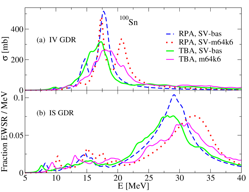
Figure 1: Comparing photo-absorption spectrum and the spectrum of the isoscalar E1 excitations from TBA and RPA for the case of ¹⁰⁰Sn computed with the two parametrizations SV-bas and SV-m64k6 and smoothing of $\Delta=400$ keV.

In previous publications, we have studied extensively giant resonance spectra in stable, doubly magic nuclei, for a systematic survey see Tselyaev et al. (2016). Two general features can be extracted. First, TBA produces some small downshift of the average resonance energy as compared to RPA. Second, and more important, the main effect of TBA is a significant smoothing of the often rather spiky RPA spectra delivering realistic spectral profiles. Figure 1 serves to demonstrate that for the example of one exotic nucleus ¹⁰⁰Sn. We consider here the GDR because this is a mode with strong spectral fragmentation where the beneficial effect of smoothing by TBA can be well seen. The RPA results show for both parametrizations strong fragmentation peaks which are so well separated that even the a posterior smoothing with $\Delta=400$ keV cannot wipe out the (unphysical) structures. TBA resolves that problem at once delivering TBA spectra with the typical GDR profile of one broad resonance peak. The key to success is that TBA induces effectively an energy-dependent smoothing because the phase space of phonon configurations increases with excitation energy.

The basic giant resonance, IS GMR and IS GQR as well as IV GDR, can be characterized by two numbers, the average peak position and the width of the resonance distribution. Resonance peak positions are evaluated as the energy centroid $E_{0}=m_{1}/m_{0}$ of the first and zeroth energy moments of the corresponding strength distributions $S(E)$ in a given energy window around the maximum. For the IV GDR (here we considered the photo absorption cross section) as well as for the IS GMR and GQR (here we considered multipole strengths), the energy windows are $E_{0}\pm 2\delta$ where $E_{0}$ is the peak position and $\delta$ is the spectral dispersion. To avoid too small energy windows, we used the constraint $\delta>\delta_{\text{min}}$ with $\delta_{\text{min}}=3$ MeV for the GMR,  2.5 MeV for the GQR, and  4 MeV for the IV GDR. The width $\Gamma$ and dispersion for these resonances were defined as

$$\Gamma=2\delta\sqrt{2\ln 2}\,,\qquad\delta^{2}=\frac{\int(E-E_{0})^{2}\,S(E)\,dE}{m_{0}}\quad.$$ (2)

The IS GDR and the PDR (low-lying dipole) strength have too complex spectra and cannot be quantified that easily. Here we cannot avoid to look at the full spectral distributions as done in sections III.3 and III.4.

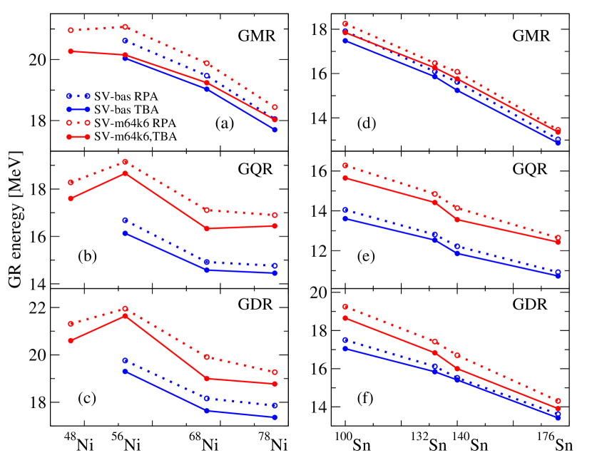
Figure 2: Mean giant resonance energies (in units of MeV) calculated for the parameter sets SV-bas (circles connected with blue lines) and SV-m64k6 (diamonds connected with red lines). The RPA results are shown with dashed line and the TBA results with solid lines. Results for Ni isotopes are shown in the left panels (a), (b), and (c) and those for Sn isotopes in the right panels (d), (e), and (f). Upper panels (a) and (d) shows GMR, middle panels (b) and (e) GQR, and lower panels (c) and (f) GDR.

Fig. 2 summarizes the average peak positions for the three basic giant resonances and the two isotopic cases considered in this paper. The effects are very similar to those observed previously in stable nuclei Tselyaev et al. (2016). With exception of the outlier ⁴⁸Ni, we see a smooth trend approximately $\propto A^{-1/3}$ as typical for most giant resonances. The trend is particularly well visible in the long Sn chain. We also see the systematic difference between SV-bas and SV-m64k6 for the GQR energies which is exclusively due to the different effective mass Brack et al. (1985); Klüpfel et al. (2009). This feature is not affected by TBA. There is an interesting slight difference between SV-bas and SV-m64k6 in the trend of the GDR. Recall that SV-m64k6 was designed to overcome Lyutorovich et al. (2012) the wrong $A$-dependence of GDR predictions seen in most Skyrme parametrizations Erler et al. (2010). This modified $A$-dependence is well visible already in the small section shown here.

The effect of phonon coupling is generally a small down-shift by phonon coupling of order 0–1 MeV, more for the lighter Ni nuclei and less for the heavier Sn series. No systematic difference between the three modes and no significant dependence on the parametrization can be seen. These typical patterns were also seen for stable nuclei Tselyaev et al. (2016). Thus far there is nothing particular is happening for this selection of exotic nuclei, even at the extremes of proton or neutron binding.

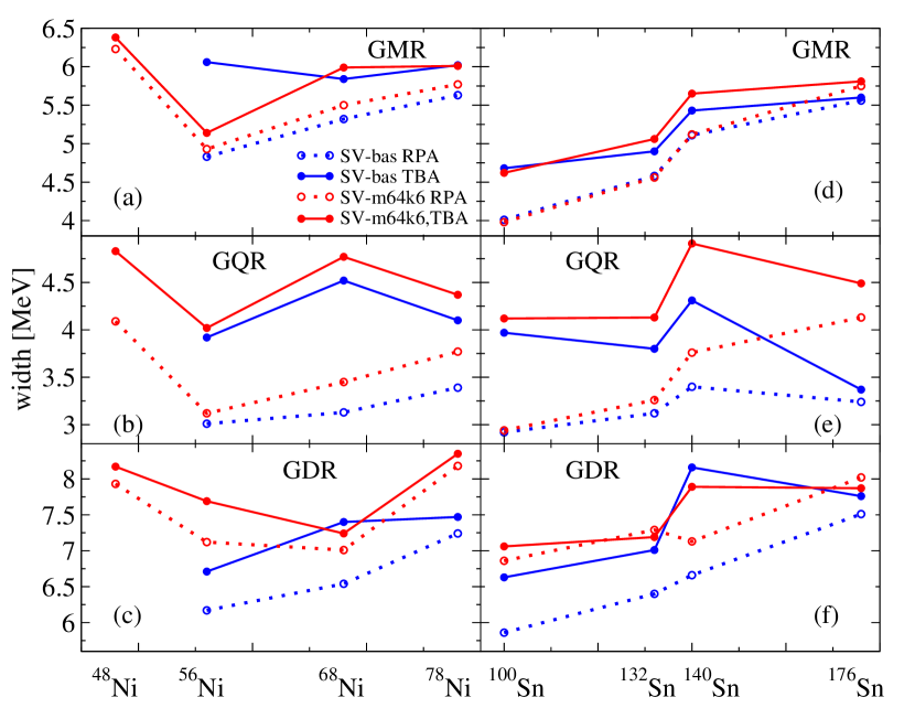
Figure 3: As Fig. 2, but for the average widths of giant resonances.

Fig. 3 complements the previous figure by showing the widths of the three resonances. Here the effects of phonon coupling are, of course, relatively stronger and lead to increase of typically 1 MeV. Not visible in this one number is the fact that this extra width is predominantly used to smooth the still peaky pattern of RPA spectra as we have seen in figure 1. It is worthwhile to note that an (energy dependent) folding with average width of 1 MeV is often used in drawing RPA results to simulate smoothing by complex configurations, see e.g. Nesterenko et al. (2002).

In case of widths, we can see some general trends (though with some exceptions): 1. Widths tend to increase along a chain with increasing neutron numbers; exception are extremely proton rich nuclei (example ⁴⁸Ni) where high density of proton states also drives larger widths. 2. SV-m64k6 with its broader spectral stretch (low effective mass) produces in RPA consistently larger widths than SV-bas; however, this trend can be overruled by phonon coupling in TBA. 3. Widths are generally increased by phonon coupling; exception are extremely neutron rich isotopes where we see practically no increase of width by phonon coupling. The reason is here that already the RPA spectra are very broadly distributed due to the high density of neutron states in these very exotic nuclei. We will look at that in detail in the next section.

III.3 Giant resonances - detailed distributions

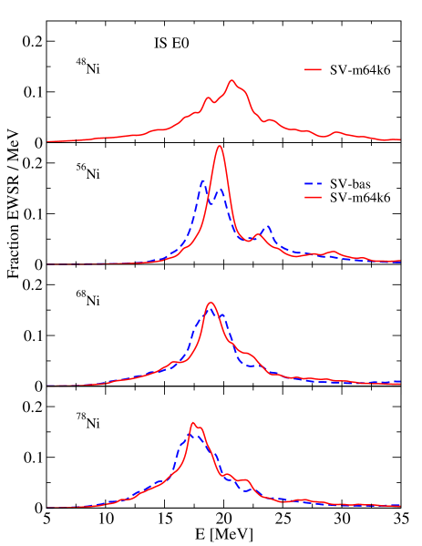
Figure 4: Isoscalar E0 strength (in units of fractions of the EWSR) in the Ni isotopes calculated in the TBA with $\Delta=400$ keV. The results for the parameter sets SV-bas and SV-m64k6 are shown by blue dashed and red full lines, respectively.

Figure 4 shows the strength distribution of the isoscalar GMR for the doubly magic Ni isotopes, ^48,56,68,78Ni, given in units of fractions of energy-weighted sum rule (EWSR) per energy interval. The general structure is similar to what was seen in stable nuclei, mostly one broad peak. There is little difference between SV-bas and SV-m64k6 which is plausible because the position of the GMR is uniquely related to the incompressibility Bohigas et al. (1979); Blaizot (1980); Klüpfel et al. (2009) and both parametrizations here have about the same incompressibility. The exotic nuclei provide a large span of isospin which allow to see more clearly trends with neutron number, or system size respectively. In this case, we see that the resonance width is rather large at the proton-rich side and shrinks by almost factor two for the neutron-rich isotopes. The peak position roughly follows the $\propto A^{-1/3}$ law known from fluid dynamical models of the GMR. We ought to remind at this place that the global trend of GMR peak positions seems not yet well under control with available SHF functionals Kvasil et al. (2016). The problem may be to some extend at the experimental side because GMR are extremely hard to identify unambiguously. Measurements of GMR in the exotic nuclei studied here are even more demanding and will probably not show up soon.

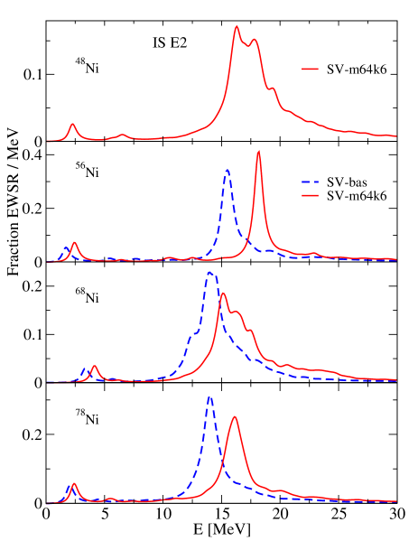
Figure 5: Same as in Fig. 4 but for the isoscalar E2 strength.

Figure 5 shows the results for the isoscalar GQR. This delivers similar pattern as seen for the GMR: one broad peak for each isotope and widths shrinking with increasing neutron number. The widths are generally somewhat smaller than for GMR, a relation which is already known from GQR and GMR in stable nuclei. For the GQR, we see a significant difference in the predictions from SV-bas and SV-m64k6. This, again, can be explained by the collective properties of the GQR which is known to depend sensitively and almost exclusively on the isoscalar effective mass Brack et al. (1985); Klüpfel et al. (2009). Recall that the effective mass of SV-m64k6 ($m^{*}/m=0.64$) is much lower than that of SV-bas ($m^{*}/m=0.9$).

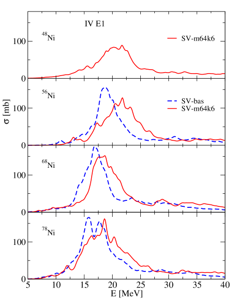
Figure 6: Same as in Fig. 4 but for the photo-absorption cross section, proportional to the energy weighted isovector dipole strength.

Figure 6 shows photo-absorption cross sections for the isovector GDR in Ni isotopes. This mode is visibly more fragmented than GMR and GQR, particularly with its long tails at high and low energies. The latter correspond to the PDR region discussed later on in section III.4. The bulk of the resonance is again represented by one broad peak. The distribution is broader than for GMR and GQR corresponding to a larger fragmentation in the GDR channel. The detailed fragmentation structure, still dominating the RPA strengths (not shown here), is wiped out by the higher configurations modeled in TBA. The comparison between SV-bas and SV-m64k6 shows an interesting effect: the average peak positions display a different isotopic trend. There is no unique agent for that because many parameters had been played with in SV-m64k4 to enforce simultaneous description of the GDR in ¹⁶O and ²⁰⁸Pb Lyutorovich et al. (2012) (which is a general problem in SHF functionals Erler et al. (2010)). But it is most likely that these different isotopic trends are the main source arranging reasonable results for the GDR in ¹⁶O (for the early presentation see Lyutorovich et al. (2012) and for results at the latest stage of model development Tselyaev et al. (2016)). The mechanisms could be worked out more deeply with studying trends of GDR on long isotopic chains. This calls for new GDR data on long chains which would be of invaluable help for fixing this particular isovector aspect of SHF functionals. Chances for such data are better than for GMR and GQR because the GDR is a dominating channel in many reactions and because precision measurements in the GDR region have become fashionable recently, see e.g. Tamii et al. (2011); Hashimoto et al. (2015).

Figs. 4 and 5 display fractions EWSR for GMR and GQR, and Fig. 7 the photo-absorption strengths for the IS GDR. The EDF parameter sets SV-bas and SV-m64k6 were used in all of these calculations, with the exception of ⁴⁸Ni. Since HF calculation with the set SV-bas does not give a bound ground state for ⁴⁸Ni (see Table 1), only the set SV-m64k6 was used in the TBA calculations for this nucleus.

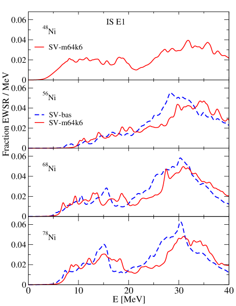
Figure 7: Same as in Fig. 4 but for the isoscalar E1 strength.

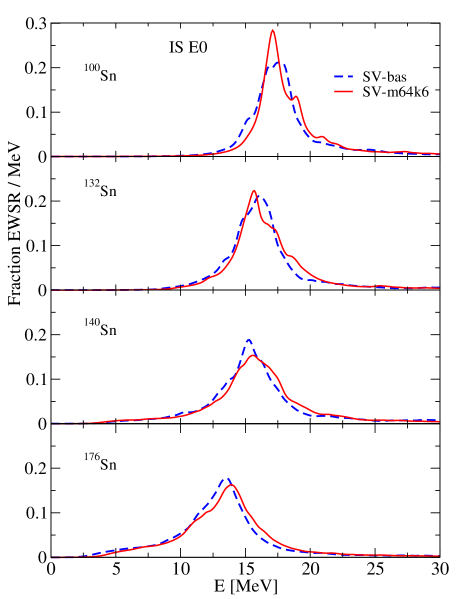
Figure 8: Same as in Fig. 4 but for the IS E0 strength in the Sn isotopes.

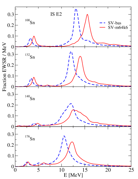
Figure 9: Same as in Fig. 4 but for the IS E2 strength in the Sn isotopes.

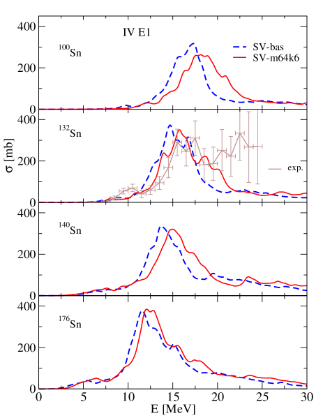
Figure 10: Same as in Fig. 4 but for the photo-absorption cross section in the Sn isotopes. The experimental data for ¹³²Sn Adrich et al. (2005) are shown by the brown line with error bars.

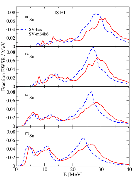
Figure 11: Same as in Fig. 4 but for the IS E1 strength in the Sn isotopes.

As the last example in the series for Ni isotopes, we look at the isoscalar dipole strength. This channel explores two interesting nuclear resonances, the compressional dipole mode at higher energies and the toroidal mode at lower energies Harakeh and van der Woude (2001). The latter one overlaps energetically with the PDR region and there is considerable cross talk between these two modes Repko et al. (2013, 2017) which makes a comparative discussion of isoscalar and isovector dipole strength extremely useful for an understanding of these low-energy dipole modes. Figure 7 shows the isoscalar dipole strength distributions for Ni isotopes computed with TBA. These strength distributions are the most widely spread of all channels discussed in this paper. The spectral fragmentation is so strong here that RPA spectra looked already as smooth as the TBA spectra shown here. There is no qualitative change of pattern nor a change of widths with the isotopes which is understandable because this channel covers two resonances which roughly maintain their position and fill the spectrum in between by fragmentation. Particularly interesting is the low-energy side, the toroidal branch, due to its cross-talk with PDR and its high sensitivity to low-lying particle-hole excitations. The latter feature is seen here from the fact that the low-energy branch of isoscalar dipole strength shows strong dependence on neutron number in the series here. The same happens, in fact, also for the low-lying isovector strength which we will see when zooming into that region in section III.4.

The same series of resonance channels is shown for the chain of doubly-magic Sn isotopes ^{100,132,140,176}Sn in Figs. 11, 11, 11, and 11. Pattern and trends are the same as in case of Ni isotopes. There is quantitative change in pattern to the extend that the widths for GMR, GQR, and GDR are all smaller than the corresponding widths for Ni. This is a known effect: the heavier the nucleus the more concentrated the giant resonances.

Experimental data are indicated for the IV GDR in ¹³²Sn. They were obtained by Coulomb dissociation of secondary Sn beams with energies around 500 MeV/nucleon Adrich et al. (2005). There is much strength at the side of higher energies which is probably unrealistic (note the large error bars). No theoretical model shows such pattern, not only ours here but also other calculations with RPA and beyond Tsoneva and Lenske (2008); Robin and Litvinova (2017); Yüksel et al. (2012). Besides this dramatic, but probably negligible, mismatch, we see that the main peak is well reproduced by SV-m64k6 and approximately by SV-bas. What is not fitting so well for both parametrizations is the pronounced low-energy peak in the data. Qualitatively, the predictions are pertinent: there is a low-lying peak, however slightly lower than data and, more important, covering less strength. The example shows that data on low-energy dipole strength (PDR region) in neutron rich nuclei provide fruitful challenges for existing nuclear models.

III.4 Low-lying dipole strength

As mentioned above, the isovector GDR strengths have remarkably long tails. Of particular interest is the low-energy tail, often called PDR. In fact, it was shown that this region, although often producing a satellite of dipole strength does not represent a single resonance, but rather a collection of $sp$ strengths of mixed nature (dipole, toroidal, compressional dipole) Repko et al. (2013, 2017); Reinhard and Nazarewicz (2013b) and as such it may be even more interesting. The $sp$ dominated, mixed structure leads to much higher sensitivity to details of the model. Thus we have a look at both, RPA and TBA, in comparison. Before we go into details we show in Fig. 12 the uncorrelated dipole strength function together with the RPA and TBA results. The sensitivity on the nuclear structure models can be seen from the uncorrelated E1 strength distributions calculated with the parameter set SV-bas and SV-m64k6, respectively. In both cases we see the well known effect of the residual interaction which shift the major part of the low-lying strength nearly 10 MeV higher creating the GDR. The phonons included in the TBA give rise to a small shift downwards and increase the width. The width of $\Delta$ = 400 keV is too large to see differences between RPA and TBA in the PDR region.

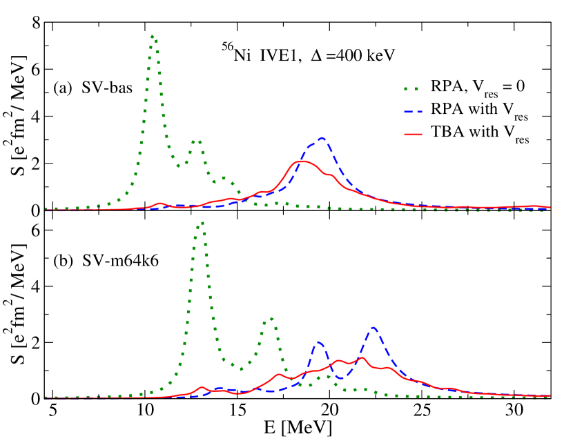
Figure 12: ⁵⁶Ni IVE1 uncorrelated strength function (green dotted line) in comparison with the RPA (blue dashed) and TBA (red solid) results. Panels (a) and (b) show the results obtained with SV-bas and SV-m64k6 forces.

Therefore we have to analyze the spectra with higher resolution. Here it helps that these low energy states experience only small broadening effects (escape width and collision width are naturally smaller there). Thus the calculations for the PDR region were performed with very small energy step 2.5 keV and small folding width $\Delta$ = 10 keV. Proper handling of nucleon continuum, as we do, is essential in these calculations near threshold. As the presentation becomes now more detailed, we have to select a subset of nuclei. For Ni isotopes (see figure 6), we concentrate on ⁵⁶Ni as proton rich isotope and ⁶⁸Ni as neutron rich isotope where in both cases dipole spectra display a marked low-energy tail. For Sn isotopes (see figure 11), we consider ¹⁰⁰Sn as proton-rich example and ¹⁴⁰Sn as a very neutron-rich exotic nucleus.

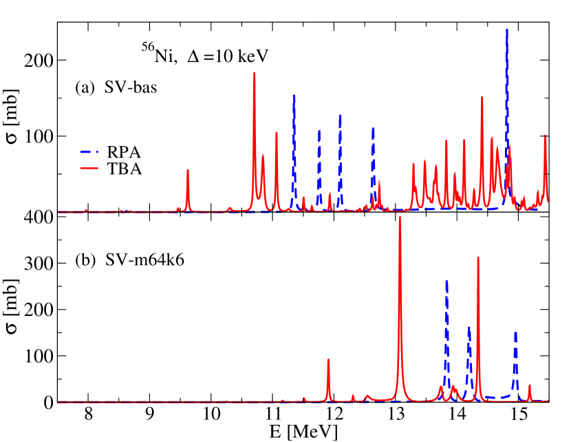
Figure 13: Fine structure of low-energy isovector dipole strength in ⁵⁶Ni: photo-absorption cross section $\sigma(E)$ calculated in RPA (blue, dashed) and TBA (red, solid) using $\Delta=10$ keV. Results for the two parameter sets SV-bas and SV-m64k6 are displayed in separate panels for better discrimination.

Figure 13 shows the low-energy wing of isovector dipole strength in ⁵⁶Ni. The lower end of the PDR spectra shows predominantly a down-shift and little fragmentation. This is due to the fact that it has a rather large HOMO-LUMO gap and therefore only very few low lying $ph$ states which, in turn, provides too few low-energy phonons. The higher part of the PDR branch (above 12 MeV) shows already some smoothing by fragmentation. It is more pronounced for SV-bas because of its higher spectral density.

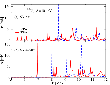
Figure 14: Same as in Fig. 13 but for ⁶⁸Ni.

Figure 14 shows the PDR part of the isovector strength for the neutron rich ⁶⁸Ni. Due to the weak neutron binding, this isotope has a long tail of low-lying neutron $ph$ states and correspondingly a couple of low-lying phonons. As a consequence, we see in TBA substantial spectral fragmentation of the isolated RPA peaks, again, more with SV-bas than with SV-m64k6. The higher resolution with which we scan the PDR spectra allows to track in detail how TBA distributes the peaks of the RPA spectrum over groups of smaller peaks. There are states which basically survive with some small down-shift in energy while others are practically dissolved and spread over the neighborhood. It is not possible to establish simple rules for that. We would also not recommend to take the details literally, peak by peak. Mind that we underestimate the effects of higher configurations which is probably not fully compensated for by the only 10 keV folding width which we use here merely to look at the spectra with higher resolution. Robust, thus more reliable, information are spectral densities and global properties of the distribution. And here we see marked differences between the two parametrizations. The distribution reaches deeper down with SV-bas than with SV-m64k6. This effect as such is established already at the level of RPA. In fact, it can be traced back to the density of mere $ph$ states. TBA modifies only details as further spectral fragmentation and possibly small energy shifts. Details which, however, should be thought of when aiming at detailed analysis.

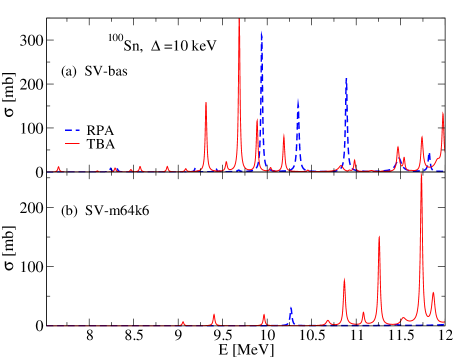
Figure 15: Same as in Fig. 13 but for ¹⁰⁰Sn. There is only one RPA peak for the set SV-m64k6 below 12 MeV because all the RPA strength for this set is above 12 MeV.

Figure 15 shows low-energy dipole spectra for the proton rich ¹⁰⁰Sn. The situation, little fragmentation and mainly down shift through TBA, looks very similar to the proton rich ⁵⁶Ni. The reason is also similar, namely the fact that in this $N=Z$ situation the spectrum of low-lying $ph$ states is very dilute. Neutrons are well bound thus having large level spacing and separation energy. Protons have small separation energy, but the Coulomb barrier produces still localized, quasi-discrete levels in the continuum which also reduces the spectral density. In case of SV-m64k6 we have a curious effect from the plotting window. We see in TBA a group of peaks at the upper end of the displayed spectrum and cannot spot the RPA ancestors. Note that these reside at somewhat higher energies just outside the plotting window. What remains the same as before is the typical difference that the SV-bas spectrum reaches deeper down than that for SV-m64k6.

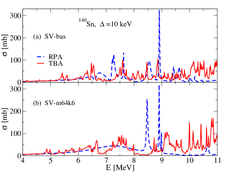
Figure 16: Same as in Fig. 13 but for ¹⁴⁰Sn.

As complement to ¹⁰⁰Sn, Fig. 16 shows low-energy dipole spectra for the very neutron rich Sn isotope ¹⁴⁰Sn. Much different than for ¹⁰⁰Sn, TBA develops here a strong bias toward spectral fragmentation leaving at the end basically a structureless broad distribution over the whole energy range shown. This is typical for nuclei toward the neutron drip line. Loosely bound neutrons produce already at mean-field level a high density of states which together with the phonons in TBA make up a considerably high density of complex configurations delivering eventually these basically flat distributions. It is, furthermore, interesting to note that, unlike previous examples, the spectra of SV-bas and SV-m64k6 cover the same energy range. This, again, happens already at RPA level. It serves as a warning that some “rules” observed in stable nuclei may fail in very exotic regions.

IV Conclusions

We investigated in the present publication the trends of giant resonances as well as the behavior of the low-lying electric dipole strength along the chains of Ni and Sn nuclei, spanning from from proton rich to very neutron isotopes. Only double magic Ni and Sn nuclei were considered.

The only exception is ¹⁴⁰Ni which has only proton magic number. But our HFB with unrestricted symmetry calculations show that even this nucleus is spherical in the ground state and that the pairing correlations have very little effect on the properties of its excited states. As theoretical tool we use a fully self-consistent treatment within the random-phase approximation (RPA) extended by particle-phonon coupling to account for many-body correlations. Our calculations are based on a recently developed version of the time-blocking approximation which allows an optimized selection of phonons and guaranties a fast convergence. This is important for a consistent treatment for all nuclei within the chains. The calculations were based on the Skyrme-Hartree-Fock (SHF) energy functional. We considered actually two previously adjusted SHF parametrizations with comparable quality in ground state properties, but different properties concerning giant resonances in order to explore the span of possible predictions. The two chains of doubly magic nuclei includes isotopes were experimental data are available and which serve nicely as benchmark for our approach. We then extended confidently our calculations to very exotic Ni and Sn isotopes which are relevant for astro-physical reaction chains.

The effects for giant resonances are the same for all isotopes along the chains and as in previous explorations of stable nuclei. The phonon coupling mainly introduces an energy dependent broadening of the spectral distributions delivering realistic pattern close to experimental distributions. There is also a small down-shift (0–1 MeV) of the average peak position.

We also investigated in detail the low-lying electric dipole strength often summarized under the label pygmy dipole resonances (PDR). Here the phonon coupling can give rise to a remarkable shift of the low energy states, redistribution of strength, and often strong fragmentation of the already much reduced dipole strength. These effect are particularly pronounced for the very neutron rich nuclei amounting there to qualitative changes of the dipole spectra. On the other side of proton rich states, phonon coupling has little influence because the density of low-energy phonon states is much lower.

As in many previous investigations, we do not observe any collective behavior in the regime of low-energy isovector dipole states. We see rather a dense sequence of states with different internal structure. The transition densities of these low-lying states show for the proton rich ⁴⁸Ni isotope proton dominated tails and for the neutron rich isotopes neutron dominated tails Lyutorovich et al. . This has, from our point of view, a simple origin: In ⁴⁸Ni the last occupied proton shell includes $sp$ states with higher spins than the closed core. The distribution of those states reaches more far outside giving rise to the observed transition densities. The same is true for the neutron rich isotopes were we observe tails which are neutron dominated.

The situation is different for the low-lying isoscalar electric dipole states. Here the major part of the $1\hbar\omega$ $ph$-strength is removed into the spurious state but due to the attractive isoscalar interaction an appreciable amount of the $3\hbar\omega$ $ph$-strength is shifted into the low-lying states. So if one is looking for some collectivity in this regime the isoscalar electric dipole might be a candidate. Further detailed analysis of the low-lying dipole spectra is presently underway.

Appendix A Numerical considerations

A.1 Single-particle basis in TBA calculations.

The size of $sp$ space is a compromise. It needs to be large enough to produce converged results and we want to have it as low as possible to render calculations affordable. In our previous calculations we checked the dependence of the results on the maximum $sp$ energy. For light (¹⁶O) and medium mass nuclei (^40,48Ca) we found saturation at $\varepsilon^{\mathrm{sp}}_{\mathrm{max}}=500$ MeV, and for heavy nuclei (¹³²Sn and ²⁰⁸Pb) at $\varepsilon^{\mathrm{sp}}_{\mathrm{max}}=100$ MeV. The present test cases of Ni and Sn isotopes lie in between, they reach deep into regimes of exotic nuclei, and they explore fine structure in the PDR region. Thus the $sp$ basis has to be inspected again. For computation of spectra of giant resonances, we find again that an $sp$ basis limited to $\varepsilon^{\mathrm{sp}}_{\mathrm{max}}=100$ MeV is sufficiently large. The calculations of dipole spectra in the low-energy regions with resolution $\Delta=10$ keV requires to increase in the $sp$-basis. We find that an upgrade from $\varepsilon^{\mathrm{sp}}_{\mathrm{max}}=100$ to 200 MeV suffices. A further increase in $\varepsilon^{\mathrm{sp}}_{\mathrm{max}}$ to 500 MeV almost does not affect the results. What $sp$ angular momentum is concerned, saturation was reached in the TBA calculations when going up to $l^{\mbox{\scriptsize sp}}_{\mbox{\scriptsize max}}$ =17 in all cases.

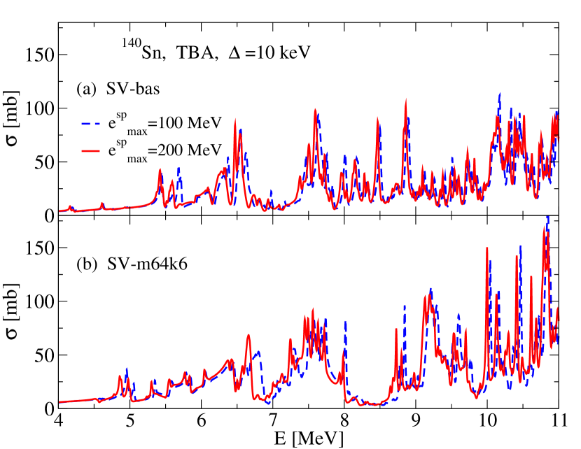
Figure 17: The effect of the $sp$-basis dimension to the cross section $\sigma(E)$ for PDR in ¹⁴⁰Sn obtained in TBA with the EDF parameter sets SV-bas and SV-m64k6 for $\varepsilon^{\mathrm{sp}}_{\mathrm{max}}=100$ and 200 MeV. $\Delta=10$ keV.

The effect of choice of $sp$ basis on the fine structure of the PDR strength is demonstrated in Fig. 17 for the case of ¹⁴⁰Sn. We still see tiny modifications when stepping from $\varepsilon^{\mathrm{sp}}_{\mathrm{max}}=100$ MeV to 200 MeV. Nothing is seen at plotting resolution for higher $\varepsilon^{\mathrm{sp}}_{\mathrm{max}}$. The choice $\varepsilon^{\mathrm{sp}}_{\mathrm{max}}=200$ MeV for low-energy spectra is clearly at the safe side. Robust moods would even have accepted the lower choice of 100 MeV.

A.2 Effect of box size

The box size was $R_{\mathrm{box}}=18$ fm for all the nuclei. Such a value gives reliable results for calculations with $\Delta=400$ keV. To investigate the influence of the box size on the fine structure of the E1 strength we have calculated this strength in RPA and TBA with $\Delta=10$ keV for $R_{\mathrm{box}}=18$ and 30 fm. These calculations were made for ¹⁰⁰Sn having small $S(p)$, ¹⁴⁰Sn having small $S(n)$, and ²⁰⁸Pb having large both the separation energies. For each of these nuclei the RPA results for $R_{\mathrm{box}}=18$ and 30 fm coincide therefore corresponding figures are of no interest.

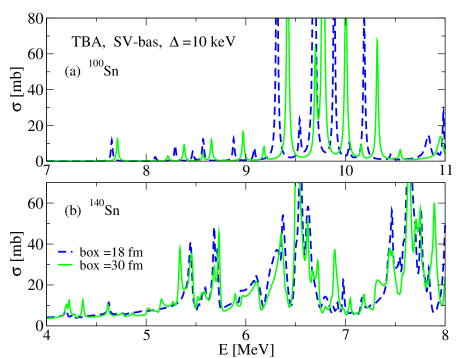
Figure 18: The box-size dependence of the photo-absorption cross section in ^100,140Sn in the low-energy region calculated in the TBA with $\Delta=10$ keV for the parameter set SV-bas.

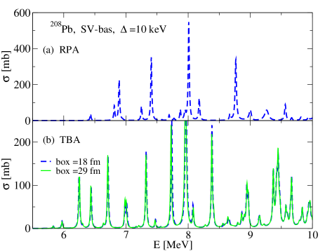
Figure 19: Same as in Fig. 19 but for ²⁰⁸Pb.

The box-size dependence of the TBA results is shown in Figs. 19 and 19. For ¹⁰⁰Sn, where $S(p)$ is small, almost twofold increase in the box size does not change the form of the TBA E1 strength in the pygmy region and only slightly, by 0.1 MeV, shifts all the peaks to high energies: see Fig. 19(a). This shift of the peaks is due by a similarly small shift in the phonon energies when changing box size. Since neither $\varepsilon^{\mathrm{sp}}_{\mathrm{max}}$, no $R_{\mathrm{box}}$ variation change the number of peaks, we conclude that for this case of ¹⁰⁰Sn all the peaks are of a physical nature. The same is found for the fine structure of the PDR in ²⁰⁸Pb obtained in TBA calculations with $\Delta=10$ keV. It does not depend on the box size, at least for $R_{\mathrm{box}}\geq 18$ fm. We expect that this holds also for all other stable nuclei.

A different picture is seen for ¹⁴⁰Sn having very small neutron separation energy $S(n)$: see Fig. 19(b). There is a noticeable (not very large) box dependence of the TBA results for the PDR fine structure. The effect is better seen in the low-energy region where the strength structure is not very complex. The main effect is an appearance of additional small peaks. The nature of these peaks may be explained if we take into account that, above the nucleon threshold, the nucleus in a box may be approximately considered as a Fermi gas in the box with infinite walls. The strength from discrete RPA (as used for the definition of phonons) for such a system has peaks whose number on a given energy interval is proportional to the size of the box. One can see a similar periodic structure in Fig. 19(b) for energies below 5.4 MeV. Here small additional TBA peaks arise because of the discrete nature of phonons in the complex configurations. The TBA peaks at $E=$ 5.4 and 5.7 MeV are probably real physical peaks. This explanation is, of course, very simplified. The main conclusion that can be drawn from this consideration is that one can not use a very small $\Delta$ in TBA calculations for a nucleus with a low nucleon separation threshold. Probably, a minimal value for the exotic Sn isotopes is $\Delta=20$ keV.

References

- Soloviev (1992) V. G. Soloviev, Theory of Atomic Nuclei: Quasiparticles and Phonons (Institute of Physics, Bristol and Philadelphia, 1992).
- Bertsch et al. (1983) G. F. Bertsch, P. F. Bortignon, and R. A. Broglia, Rev. Mod. Phys. 55, 287 (1983).
- Kamerdzhiev et al. (2004) S. P. Kamerdzhiev, J. Speth, and G. Tertychny, Phys. Rep. 393, 1 (2004).
- Tselyaev et al. (2017) V. Tselyaev, N. Lyutorovich, J. Speth, and P.-G. Reinhard, Phys. Rev. C 96, 024312 (2017).
- Vdovin and Soloviev (1983) A. I. Vdovin and V. G. Soloviev, Sov. J. Part. Nucl. 14, 99 (1983).
- Voronov and Soloviev (1983) V. V. Voronov and V. G. Soloviev, Sov. J. Part. Nucl. 14, 583 (1983).
- Dehesa et al. (1977) J. S. Dehesa, S. Krewald, J. Speth, and A. Faessler, Phys. Rev. C 15, 1858 (1977).
- Colò et al. (1994) G. Colò, N. Van Giai, P. F. Bortignon, and R. A. Broglia, Phys. Rev. C 50, 1496 (1994).
- Colò and Bortignon (2001) G. Colò and P. F. Bortignon, Nucl. Phys. A 687, 282c (2001).
- Roca-Maza et al. (2017) X. Roca-Maza, Y. F. Niu, G. Colò, and P. F. Bortignon, J. Phys. G: Nucl. Part. Phys. 44, 044001 (2017).
- Barbieri and Dickhoff (2003) C. Barbieri and W. H. Dickhoff, Phys. Rev. C 68, 014311 (2003).
- Dickhoff and Barbieri (2004) W. H. Dickhoff and C. Barbieri, Prog. Part. Nucl. Phys. 52, 377 (2004).
- Tselyaev (1989) V. I. Tselyaev, Sov. J. Nucl. Phys. 50, 780 (1989).
- Kamerdzhiev et al. (1993) S. P. Kamerdzhiev, J. Speth, G. Tertychny, and V. Tselyaev, Nucl. Phys. A 555, 90 (1993).
- Tselyaev (2007) V. I. Tselyaev, Phys. Rev. C 75, 024306 (2007).
- Litvinova et al. (2007) E. Litvinova, P. Ring, and V. Tselyaev, Phys. Rev. C 75, 064308 (2007).
- Litvinova et al. (2008) E. Litvinova, P. Ring, and V. Tselyaev, Phys. Rev. C 78, 014312 (2008).
- Lyutorovich et al. (2015) N. Lyutorovich, V. Tselyaev, J. Speth, S. Krewald, F. Grümmer, and P.-G. Reinhard, Phys. Lett. B 749, 292 (2015).
- Lyutorovich et al. (2016) N. Lyutorovich, V. Tselyaev, J. Speth, S. Krewald, and P.-G. Reinhard, Phys. At. Nucl. 79, 868 (2016).
- Tselyaev et al. (2016) V. Tselyaev, N. Lyutorovich, J. Speth, S. Krewald, and P.-G. Reinhard, Phys. Rev. C 94, 034306 (2016).
- Tselyaev et al. (2018) V. Tselyaev, N. Lyutorovich, J. Speth, and P.-G. Reinhard, Phys. Rev. C 97, 044308 (2018).
- Arnould et al. (2007) M. Arnould, S. Goriely, and K. Takahashi, Physics Reports 450, 97 (2007).
- Reinhard and Nazarewicz (2013a) P. G. Reinhard and W. Nazarewicz, Phys. Rev. C 87, 014324 (2013a).
- Yao et al. (2015) J. M. Yao, M. Bender, and P.-H. Heenen, Phys. Rev. C 91, 024301 (2015).
- Saxena and Kaushik (2017) G. Saxena and M. Kaushik, Chin. J. Phys. 55, 1149 (2017), arXiv:1704.08421 [nucl-th] .
- Wieland et al. (2009) O. Wieland, A. Bracco, F. Camera, G. Benzoni, N. Blasi, S. Brambilla, F. C. L. Crespi, S. Leoni, B. Million, R. Nicolini, A. Maj, P. Bednarczyk, J. Grebosz, M. Kmiecik, W. Meczynski, J. Styczen, T. Aumann, A. Banu, T. Beck, F. Becker, L. Caceres, P. Doornenbal, H. Emling, J. Gerl, H. Geissel, M. Gorska, O. Kavatsyuk, M. Kavatsyuk, I. Kojouharov, N. Kurz, R. Lozeva, N. Saito, T. Saito, H. Schaffner, H. J. Wollersheim, J. Jolie, P. Reiter, N. Warr, G. deAngelis, A. Gadea, D. Napoli, S. Lenzi, S. Lunardi, D. Balabanski, G. LoBianco, C. Petrache, A. Saltarelli, M. Castoldi, A. Zucchiatti, J. Walker, and A. Bürger, Phys. Rev. Lett. 102, 092502 (2009).
- Wieland and Bracco (2011) O. Wieland and A. Bracco, Progress in Particle and Nuclear Physics 66, 374 (2011), particle and Nuclear Astrophysics.
- Vandebrouck et al. (2014) M. Vandebrouck, J. Gibelin, E. Khan, N. L. Achouri, H. Baba, D. Beaumel, Y. Blumenfeld, M. Caamaño, L. Càceres, G. Colò, F. Delaunay, B. Fernandez-Dominguez, U. Garg, G. F. Grinyer, M. N. Harakeh, N. Kalantar-Nayestanaki, N. Keeley, W. Mittig, J. Pancin, R. Raabe, T. Roger, P. Roussel-Chomaz, H. Savajols, O. Sorlin, C. Stodel, D. Suzuki, and J. C. Thomas, Phys. Rev. Lett. 113, 032504 (2014).
- Hamamoto and Sagawa (2014) I. Hamamoto and H. Sagawa, Phys. Rev. C 90, 031302 (2014).
- Paar et al. (2005) N. Paar, P. Papakonstantinou, V. Ponomarev, and J. Wambach, Physics Letters B 624, 195 (2005).
- Papakonstantinou et al. (2014) P. Papakonstantinou, H. Hergert, V. Y. Ponomarev, and R. Roth, Phys. Rev. C 89, 034306 (2014).
- Papakonstantinou et al. (2015a) P. Papakonstantinou, H. Hergert, V. Y. Ponomarev, and R. Roth, Phys. Rev. C 91, 029903 (2015a).
- Papakonstantinou et al. (2015b) P. Papakonstantinou, H. Hergert, and R. Roth, Phys. Rev. C 92, 034311 (2015b).
- Co’ et al. (2013) G. Co’, V. De Donno, M. Anguiano, and A. M. Lallena, Phys. Rev. C 87, 034305 (2013).
- Avdeenkov et al. (2011) A. Avdeenkov, S. Goriely, S. Kamerdzhiev, and S. Krewald, Phys. Rev. C 83, 064316 (2011).
- Hagen et al. (2016) G. Hagen, G. R. Jansen, and T. Papenbrock, Phys. Rev. Lett. 117, 172501 (2016).
- Robin and Litvinova (2017) C. Robin and E. Litvinova, Proceedings, 5th Conference on Nuclei and Mesoscopic Physics (NMP17): East Lansing, Michigan, USA, March 6-10, 2017, AIP Conf. Proc. 1912, 020014 (2017), arXiv:1709.03606 [nucl-th] .
- Sun et al. (2018) X.-W. Sun, J. Chen, and D.-H. Lu, Chinese Physics C 42, 014101 (2018).
- Kim and Papakonstantinou (2016) Y. Kim and P. Papakonstantinou, Eur. Phys. J. A 52, 176 (2016).
- Morris et al. (2018) T. D. Morris, J. Simonis, S. R. Stroberg, C. Stumpf, G. Hagen, J. D. Holt, G. R. Jansen, T. Papenbrock, R. Roth, and A. Schwenk, Phys. Rev. Lett. 120, 152503 (2018).
- Colò et al. (2014) G. Colò, U. Garg, and H. Sagawa, The European Physical Journal A 50, Article: 26 (2014).
- Pomorski et al. (2014) M. Pomorski, M. Pfützner, W. Dominik, R. Grzywacz, A. Stolz, T. Baumann, J. S. Berryman, H. Czyrkowski, R. Dabrowski, A. Fijałkowska, T. Ginter, J. Johnson, G. Kamiński, N. Larson, S. N. Liddick, M. Madurga, C. Mazzocchi, S. Mianowski, K. Miernik, D. Miller, S. Paulauskas, J. Pereira, K. P. Rykaczewski, and S. Suchyta, Phys. Rev. C 90, 014311 (2014).
- Bender et al. (2003) M. Bender, P.-H. Heenen, and P.-G. Reinhard, Rev. Mod. Phys. 75, 121 (2003).
- Stone and Reinhard (2007) J. R. Stone and P. . G. Reinhard, Prog. Part. Nucl. Phys. 58, 587 (2007), http://www.arxiv.org/abs/nucl-th/0607002.
- Erler et al. (2011) J. Erler, P. Klüpfel, and P. G. Reinhard, J. Phys. G 38, 033101 (2011).
- Klüpfel et al. (2009) P. Klüpfel, P. G. Reinhard, T. J. Bürvenich, and J. A. Maruhn, Phys. Rev. C 79, 034310 (2009).
- Lyutorovich et al. (2012) N. Lyutorovich, V. I. Tselyaev, J. Speth, S. Krewald, F. Grümmer, and P. G. Reinhard, Phys. Rev. Lett. 109, 092502 (2012).
- Toepffer and Reinhard (1988) C. Toepffer and P.-G. Reinhard, Ann. Phys. (N.Y.) 181, 1 (1988).
- Tselyaev (2013) V. I. Tselyaev, Phys. Rev. C 88, 054301 (2013).
- Brack et al. (1985) M. Brack, C. Guet, and H.-B. Håkansson, Phys. Rep. 123, 275 (1985).
- Erler et al. (2010) J. Erler, P. Klüpfel, and P.-G. Reinhard, J. Phys. G 37, 064001 (2010), http://www.arxiv.org/abs/1002.0027.
- Nesterenko et al. (2002) V. O. Nesterenko, J. Kvasil, and P.-G. Reinhard, Phys. Rev. C 66, 044307 (2002), http://www.arxiv.org/abs/nucl-th/0204018.
- Bohigas et al. (1979) O. Bohigas, A. M. Lane, and J. Martorell, Phys. Rep. 51, 267 (1979).
- Blaizot (1980) J. P. Blaizot, Phys. Rep. 64, 171 (1980).
- Kvasil et al. (2016) J. Kvasil, V. O. Nesterenko, A. Repko, W. Kleinig, and P.-G. Reinhard, Phys. Rev. C 94, 064302 (2016).
- Tamii et al. (2011) A. Tamii, I. Poltoratska, P. von Neumann-Cosel, Y. Fujita, T. Adachi, C. A. Bertulani, J. Carter, M. Dozono, H. Fujita, K. Fujita, K. Hatanaka, D. Ishikawa, M. Itoh, T. Kawabata, Y. Kalmykov, A. M. Krumbholz, E. Litvinova, H. Matsubara, K. Nakanishi, R. Neveling, H. Okamura, H. J. Ong, B. Özel-Tashenov, V. Y. Ponomarev, A. Richter, B. Rubio, H. Sakaguchi, Y. Sakemi, Y. Sasamoto, Y. Shimbara, Y. Shimizu, F. D. Smit, T. Suzuki, Y. Tameshige, J. Wambach, R. Yamada, M. Yosoi, and J. Zenihiro, Phys. Rev. Lett. 107, 062502 (2011).
- Hashimoto et al. (2015) T. Hashimoto, A. M. Krumbholz, P.-G. Reinhard, A. Tamii, P. von Neumann-Cosel, T. Adachi, N. Aoi, C. A. Bertulani, H. Fujita, Y. Fujita, E. Ganio, K. Hatanaka, E. Ideguchi, C. Iwamoto, T. Kawabata, N. T. Khai, A. Krugmann, D. Martin, H. Matsubara, K. Miki, R. Neveling, H. Okamura, H. J. Ong, I. Poltoratska, V. Y. Ponomarev, A. Richter, H. Sakaguchi, Y. Shimbara, Y. Shimizu, J. Simonis, F. D. Smit, G. Süsoy, T. Suzuki, J. H. Thies, M. Yosoi, and J. Zenihiro, Phys. Rev. C 92, 031305(R) (2015).
- Adrich et al. (2005) P. Adrich, A. Klimkiewicz, M. Fallot, K. Boretzky, T. Aumann, D. Cortina-Gil, U. DattaPramanik, T. W. Elze, H. Emling, H. Geissel, M. Hellström, K. L. Jones, J. V. Kratz, R. Kulessa, Y. Leifels, C. Nociforo, R. Palit, H. Simon, G. Surówka, K. Sümmerer, and W. Walus (LAND-FRS Collaboration), Phys. Rev. Lett. 95, 132501 (2005).
- Harakeh and van der Woude (2001) M. N. Harakeh and A. van der Woude, Giant Resonances: Fundamental High-Frequency Modes of Nuclear Excitation (Oxford University Press, 2001).
- Repko et al. (2013) A. Repko, P.-G. Reinhard, V. Nesterenko, and J. Kvasil, Phys. Rev. C 87, 024305 (2013), arXiv:1212.2088.
- Repko et al. (2017) A. Repko, J. Kvasil, V. Nesterenko, and P.-G. Reinhard, Eur. Phys. J A 53, 221 (2017), arXiv:1705.05436.
- Tsoneva and Lenske (2008) N. Tsoneva and H. Lenske, Phys. Rev. C 77, 024321 (2008).
- Yüksel et al. (2012) E. Yüksel, E. Khan, and K. Bozkurt, Nuclear Physics A 877, 35 (2012).
- Reinhard and Nazarewicz (2013b) P.-G. Reinhard and W. Nazarewicz, Phys. Rev. C 87, 014324 (2013b).
- (65) N. Lyutorovich, V. Tselyaev, J. Speth, and P.-G. Reinhard, in preparation.