Character-Aware Decoder for Translation
into Morphologically Rich Languages

Abstract

Neural machine translation (NMT) systems operate primarily on words (or subwords), ignoring lower-level patterns of morphology. We present a character-aware decoder designed to capture such patterns when translating into morphologically rich languages. We achieve character-awareness by augmenting both the softmax and embedding layers of an attention-based encoder-decoder model with convolutional neural networks that operate on the spelling of a word. To investigate performance on a wide variety of morphological phenomena, we translate English into $14$ typologically diverse target languages using the TED multi-target dataset. In this low-resource setting, the character-aware decoder provides consistent improvements with BLEU score gains of up to $+3.05$. In addition, we analyze the relationship between the gains obtained and properties of the target language and find evidence that our model does indeed exploit morphological patterns.

1 Introduction

Traditional attention-based encoder-decoder neural machine translation (NMT) models learn word-level embeddings, with a continuous representation for each unique word type [Bahdanau et al., 2015]. However, this results in a long tail of rare words for which we do not learn good representations. More recently, it has become standard practice to mitigate the vocabulary size problem with Byte-Pair Encoding (BPE) [Gage, 1994, Sennrich et al., 2016]. BPE iteratively merges consecutive characters into larger chunks based on their frequency, which results in the breaking up of less common words into “subword units.”

While BPE addresses the vocabulary size problem, the spellings of the subword units are still ignored. On the other hand, purely character-level NMT translates one character at a time and can implicitly learn about morphological patterns within words as well as generalize to unseen vocabulary. Recently, ?) show that very deep character-level models can outperform BPE, however, the smallest data size evaluated was 2 million sentences, so it is unclear if the results hold for low-resource settings and when translating into a range of different morphologically rich languages. Furthermore, tuning deep character-level models is expensive, even for low-resource settings. Deep character-level models are sensitive to the dropout rate and tuning takes much longer due to longer sequence lengths [Cherry et al., 2018].

A middle-ground alternative is character-aware word-level modeling. Here, the NMT system operates over words but uses word embeddings that are sensitive to spellings and thereby has the ability to learn morphological patterns in the language. Such character-aware approaches have been applied successfully in NMT to the source-side word embedding layer [Costa-jussà and Fonollosa, 2016], but surprisingly, similar gains have not been achieved on the target side [Belinkov et al., 2017].

While source-side character-aware models only need to make the source embedding layer character-aware, on the target-side we require both the target embedding layer and the softmax layer to be character-aware, which presents additional challenges. We find that the trivial application of methods from ?) to these target-side embeddings results in significant drop in performance. Instead, we propose mixing compositional and standard word embeddings via a gating function. While simple, we find it is critical to successful target-side character awareness.

It is worth noting that unlike some purely character-level methods our aim is not to generate novel words, though this method can function on top of subword methods which do so [Shapiro and Duh, 2018]. Rather, the character-aware representations decrease the sparsity of embeddings for rare words or subwords, which are a problem in low-resource morphologically rich settings. We summarize our contribution as follows:

1. We propose a method for utilizing character-aware embeddings in an NMT decoder that can be used over word or subword sequences.

2. We explore how our method interacts with BPE over a range of merge operations (including word-level and purely character-level) and highlight that there is no “typical BPE” setting for low-resource NMT.

3. We evaluate our model on $14$ target languages and observe consistent improvements over baselines. Furthermore, we analyze to what extent the success of our method corresponds to improved handling of target language morphology.

2 Related Work

NMT has benefited from character-aware word representations on the source side [Costa-jussà and Fonollosa, 2016], which follows language modeling work by ?) and generate source-side input embeddings using a CNN over the character sequence of each word. Further analysis revealed that hidden states of such character-aware models have increased knowledge of morphology  [Belinkov et al., 2017]. They additionally try using character-aware representations in the target side embedding layer, leaving the softmax matrix with standard word representations, and found no improvements.

Our work is also aligned with the character-aware models proposed in [Kim et al., 2016], but we additionally employ a gating mechanism between character-aware representations and standard word representations similar to language modeling work by [Miyamoto and Cho, 2016]. However, our gating is a learned type-specific vector rather than a fixed hyperparameter.

There is additionally a line of work on purely character-level NMT, which generates words one character at a time [Ling et al., 2015, Chung et al., 2016, Passban et al., 2018]. While initial results here were not strong, ?) revisit this with deeper architectures and sweeping dropout parameters and find that they outperform BPE across settings of the merge hyperparameter. They examine different data sizes and observe improvements in the smaller data size settings—however, the smallest size is about 2 million sentence pairs. In contrast, we look at a smaller order of magnitude data size and present an alternate approach which doesn’t require substantial tuning of parameters across different languages.

Finally, Byte-Pair Encoding (BPE) [Sennrich et al., 2016] has become a standard preprocessing step in NMT pipelines and provides an easy way to generate sequences with a mixture of full words and word fragments. Note that BPE splits are agnostic to any morphological pattern present in the language, for example the token politely in our dataset is split into pol+itely, instead of the linguistically plausible split polite+ly. Our approach can be applied to word-level sequences and sequences at any BPE merge hyperparameter greater than $0$. Increasing the hyperparameter results in more words and longer subwords that can exhibit morphological patterns. Our goal is to exploit these morphological patterns and enrich the word (or subword) representations with character-awareness.

3 Encoder-Decoder NMT

An attention-based encoder-decoder network [Bahdanau et al., 2015, Luong et al., 2015] models the probability of a target sentence ${\boldsymbol{\mathbf{y}}}$ of length $J$ given a source sentence ${\boldsymbol{\mathbf{x}}}$ as:

$$p({\boldsymbol{\mathbf{y}}}\mid{\boldsymbol{\mathbf{x}}}) =\prod_{j=1}^{J}p(y_{j}\mid{\boldsymbol{\mathbf{y}}}_{0:j-1},{\boldsymbol{\mathbf{x}}};{\boldsymbol{\mathbf{\theta}}})$$ (1)

where ${\boldsymbol{\mathbf{\theta}}}$ represents all the parameters of the network. At each time-step the $j^{\prime}$th output token is generated by:

$$p(y_{j}\mid{\boldsymbol{\mathbf{y}}}_{0:j-1},{\boldsymbol{\mathbf{x}}})=\text{softmax}({\boldsymbol{\mathbf{W_{o}}}}{\boldsymbol{\mathbf{s}}}_{j})$$ (2)

where ${\boldsymbol{\mathbf{s}}}_{j}\in\mathbb{R}^{D\times 1}$ is the decoder hidden state at time $j$ and ${\boldsymbol{\mathbf{W_{o}}}}\in\mathbb{R}^{\lvert\mathcal{V}\rvert\times D}$ is the weight matrix of the softmax layer, which provides a continuous representation for target words. ${\boldsymbol{\mathbf{s}}}_{j}$ is computed using the following recurrence:

$${\boldsymbol{\mathbf{s}}}_{j} =\text{tanh}({\boldsymbol{\mathbf{W_{c}}}}\;[{\boldsymbol{\mathbf{c}}}_{j};{\boldsymbol{\mathbf{\tilde{s}}}}_{j}])$$ (3)

$${\boldsymbol{\mathbf{\tilde{s}}}}_{j} =f([{\boldsymbol{\mathbf{s}}}_{j-1};{\boldsymbol{\mathbf{w_{s}}}}^{y_{j-1}};{\boldsymbol{\mathbf{\tilde{s}}}}_{j-1}])$$ (4)

where $f$ is an LSTM cell. ${\boldsymbol{\mathbf{W_{s}}}}\in\mathbb{R}^{\lvert\mathcal{V}\rvert\times E}$ is the target-side embedding matrix, which provides continuous representations for the previous target word when used as input to the RNN. Here, ${\boldsymbol{\mathbf{w_{s}}}}^{y_{j-1}}\in\mathbb{R}^{1\times E}$ is a row vector from the embedding matrix ${\boldsymbol{\mathbf{W_{s}}}}$ corresponding to the value of $y_{j-1}$. $\mathcal{V}$ is the target vocabulary set, $D$ is the is the RNN size and $E$ is embedding size. Often these matrices ${\boldsymbol{\mathbf{W_{o}}}}$ and ${\boldsymbol{\mathbf{W_{s}}}}$ are tied.

The context vector ${\boldsymbol{\mathbf{c}}}_{j}$ is obtained by taking a weighted average over the concatenation of a bidirectional RNN encoder’s hidden states.

$${\boldsymbol{\mathbf{c}}}_{j} =\sum_{i=1}^{{I}}\alpha_{i},{\boldsymbol{\mathbf{h}}}_{i}$$ (5)

$$\alpha_{i} =\frac{\exp{({\boldsymbol{\mathbf{s}}}_{j}^{T}{\boldsymbol{\mathbf{W_{a}}}}{\boldsymbol{\mathbf{h}}}_{i})}}{\sum_{l}\exp{({\boldsymbol{\mathbf{s}}}_{j}^{T}{\boldsymbol{\mathbf{W_{a}}}}{\boldsymbol{\mathbf{h}}}_{l}})}$$ (6)

The attention matrix ${\boldsymbol{\mathbf{W_{a}}}}\in\mathbb{R}^{D\times H}$ is learned jointly with the model, multiplying with the previous decoder state and bidirectional encoder state ${\boldsymbol{\mathbf{h}}}_{i}\in\mathbb{R}^{H\times 1}$, normalized over encoder hidden states via the softmax operation.

4 Character-Aware Extension

In this section we detail the incorporation of character-awareness into the two decoder embedding matrices ${\boldsymbol{\mathbf{W_{o}}}}$ and ${\boldsymbol{\mathbf{W_{s}}}}$. To begin, we consider an example target side word (or subword in the case of preprocessing with BPE), cat. In both ${\boldsymbol{\mathbf{W_{o}}}}$ and ${\boldsymbol{\mathbf{W_{s}}}}$, there exist row vectors, ${\boldsymbol{\mathbf{w_{o}}}}^{\texttt{cat}}$ and ${\boldsymbol{\mathbf{w_{s}}}}^{\texttt{cat}}$ that contain the continuous vector representation for the word cat. In a traditional NMT system, these vectors are learned as the entire network tries to maximize the objective in Equation 1. The objective does not require the vectors ${\boldsymbol{\mathbf{w_{o}}}}^{\texttt{cat}}$ and ${\boldsymbol{\mathbf{w_{s}}}}^{\texttt{cat}}$ to model any aspect of the spelling of the word. Figure 1a illustrates a simple non-compositional word embedding.

At a high level, we can view our notion of character-awareness as a composition function $\text{comp}(.;{\boldsymbol{\mathbf{\omega}}})$, parameterized by ${\boldsymbol{\mathbf{\omega}}}$, that takes the character sequence that makes up a word (i.e. its spelling) as input and then produces a continuous vector representation:

$${\boldsymbol{\mathbf{w}}}_{\text{comp}}^{\texttt{cat}} =\text{comp}(\langle s\rangle,\texttt{c},\texttt{a},\texttt{t},\langle/s\rangle;{\boldsymbol{\mathbf{\omega}}})$$ (7)

${\boldsymbol{\mathbf{\omega}}}$ is learned jointly with the overall objective. Special characters $\langle s\rangle$ and $\langle/s\rangle$ denote the beginning and end of sequence respectively.

Figure 1b illustrates our compositional approach to generating embeddings [Kim et al., 2016]. First, a character-embedding layer converts the spelling of a word into a sequence of character embeddings. Next, we apply $4$ convolution operations, with kernel sizes $3,4,5$ and $6$, over the character sequence and the resulting output matrix is max-pooled. We set the output channel size of each convolution to $\frac{1}{4}$ of the final desired embedding size. The max-pooled vector from each convolution is concatenated to create the composed word representation. Finally, we add highway layers to obtain the final embeddings.

(a)

(b)

Figure 1: Different approaches to generating embeddings. (a) standard word embedding that treats words as a single symbol. (b) CNN-based composition function. We use multiple CNNs with different kernel sizes over the character embeddings. The resulting hidden states are combined into a single word embedding via max pooling. Note that (b) shows only $2$ convolution filters for clarity, in practice we use 4.

4.1 Composed & Standard Gating

The composition is applied to every type in the vocabulary and thus generates a complete embedding matrix (and softmax matrix). In doing so, we assume that every word in the vocabulary has a vector representation that can be composed from its spelling sequence. This is a strong assumption as many words, in particular high frequency words, are not normally compositional, e.g. the substring ing in thing is not compositional in the way that it is in running. Thus, we mix the compositional and standard embedding vectors. We expect standard embeddings to better represent the meaning of certain words, such has function words and other high-frequency words. For each word $v$ in the vocabulary we also learn a gating vector ${\boldsymbol{\mathbf{g}}}^{v}\in[0,1]^{1\times D}$.

$${\boldsymbol{\mathbf{g}}}^{v} =\sigma({\boldsymbol{\mathbf{w}}}_{\text{gate}}^{v})$$ (8)

Where, $\sigma$ is a sigmoid operation and type-specific parameters ${\boldsymbol{\mathbf{w}}}_{\text{gate}}^{v}$ are jointly learned along with all the other parameters of the composition function. These parameters are regularized to remain close to ${\boldsymbol{\mathbf{0}}}$ using dropout. Our final mixed word representation for each word $v\in\mathcal{V}$ is given by:

$${\boldsymbol{\mathbf{w}}}^{v}_{\text{mix}}={\boldsymbol{\mathbf{g}}}^{v}\odot{\boldsymbol{\mathbf{w}}}^{v}_{\text{std}}+({\boldsymbol{\mathbf{1.}}}-{\boldsymbol{\mathbf{g}}}^{v})\odot{\boldsymbol{\mathbf{w}}}^{v}_{\text{comp}}$$ (9)

Where ${\boldsymbol{\mathbf{w}}}^{v}_{\text{mix}}$ is the final word embedding, ${\boldsymbol{\mathbf{w}}}^{v}_{\text{std}}$ is the standard word embedding, ${\boldsymbol{\mathbf{w}}}^{v}_{\text{comp}}$ is the embedding by the composition function and ${\boldsymbol{\mathbf{g}}}^{v}$ is the type-specific gating vector for the $v$’th word. The weight matrix is obtained by stacking the word vectors for each word $v\in\mathcal{V}$. The same representation is used for the target embedding layer and the softmax layer i.e. we set ${\boldsymbol{\mathbf{w_{o}}}}^{\texttt{cat}}={\boldsymbol{\mathbf{w_{s}}}}^{\texttt{cat}}={\boldsymbol{\mathbf{w}}}_{\text{mix}}^{\texttt{cat}}$, when $v=\texttt{cat}$. Thus, tying the composition function parameters for the softmax weight matrix and the target-side embedding matrix.

Experiments comparing the standard embedding model and the compositional embedding model with and without gating are summarized in Table 1. Row “C” shows the performance of naively using the composition function (which works in the source-side) on the target-side. We observe a catastrophic drop in BLEU ($-14.62$) compared to a standard NMT encoder-decoder. The Character-aware gated model(CG), however, outperforms the baseline by $0.91$ BLEU points suggesting that the CNN composition function and standard embeddings work in a complementary fashion.

Composition Method	BLEU
Std.- (no composition)	26.84
CGS (without gating)	12.22
CG (target embedding only)	26.61
CG (softmax embedding only)	27.16
CG (both)	27.75

Table 1: Experiments to determine the effectiveness of composition based embeddings and gated embeddings. We used en-de language pair from the TED multi-target dataset. Std. is our baseline with standard word embeddings, model C is the composition only model and CG combines the character-aware (composed) embedding and standard embedding via a gating function.

4.2 Large Vocabulary Approximation

In Equation 2 of the general NMT framework, the softmax operation generates a distribution over the output vocabulary. Our character-aware model requires a much larger computation graph as we apply convolutions (and highway layers) over the spellings (character embeddings) of entire target vocabulary, placing a limitation on the target vocabulary size for our model. Which is problematic for word-level modeling (without BPE).

To make our character-aware model accommodate large target vocabulary sizes, we incorporate an approximation mechanism based on [Jean et al., 2015]. Instead of computing the softmax over the entire vocabulary, we uniformly sample $20$k vocabulary types and the vocabulary types that are present in the training batch.

During decoding, we compute the forward pass ${\boldsymbol{\mathbf{W_{o}}}}{\boldsymbol{\mathbf{s}}}_{j}$ in Equation 2 in several splits of the target vocabulary. As no backward pass is required we clear the memory (i.e. delete the computation graph) after each split is computed.

5 Experiments

Language	BPE Sweep			@ $30$k BPE			@ Word-level
	Std(Best BPE)	CG(Best BPE)	$\Delta$	Std	CG	$\Delta$	Std	CG	$\Delta$
cs	20.57 (7.5k)	21.41 (7.5k)	+0.84	18.73	21.28	+2.55	18.44	21.49	+3.05
uk	15.79 (7.5k)	16.60 (30k)	+0.81	14.27	16.60	+2.33	12.94	15.30	+2.36
pl	16.76 (15k)	18.00 (30k)	+1.24	15.98	18.00	+2.02	15.49	17.20	+1.71
tr	15.11 (7.5k)	15.83 (30k)	+0.72	13.82	15.83	+2.01	12.58	14.75	+2.17
hu	16.61 (3.2k)	17.23 (15k)	+0.62	15.45	17.21	+1.76	14.18	16.52	+2.34
he	23.36 (3.2k)	23.86 (30k)	+0.50	22.47	23.86	+1.39	21.26	23.01	+1.75
pt	37.85 (15k)	38.35 (30k)	+0.50	37.05	38.35	+1.30	37.13	38.36	+1.23
ar	16.22 (7.5k)	16.28 (30k)	+0.06	15.05	16.28	+1.23	14.45	16.05	+1.60
de	27.37 (7.5k)	28.12 (30k)	+0.75	26.94	28.12	+1.21	26.84	27.75	+0.91
ro	24.02 (3.2k)	24.20 (15k)	+0.18	22.88	24.00	+1.12	22.39	23.27	+0.88
bg	31.63 (7.5k)	32.20 (15k)	+0.57	30.92	31.90	+0.98	30.18	31.43	+1.25
fr	35.97 (1.6k)	36.17 (7.5k)	+0.20	35.31	35.92	+0.61	35.28	36.01	+0.73
fa	12.94 (30k)	13.52 (30k)	+0.58	12.94	13.52	+0.58	12.85	12.79	-0.06
ru	19.28 (30k)	19.61 (30k)	+0.33	19.28	19.61	+0.33	17.60	19.04	+1.44

Table 2: Best BLEU scores swept over $6$ different BPE merge setting ($1.6$k, $3.2$k, $7.5$k, $15$k, $30$k, $60$k), and at a standard setting of $30$k. We notice a consistent improvement across languages and settings of the merge operation parameter.

We evaluate our character aware model on $14$ different languages in a low-resource setting. Additionally, we sweep over several BPE merge hyperparameter settings from character-level to fully word-level for both our model and the baseline and find consistent gains in the character-aware model over the baseline. These gains are stable across all BPE merge hyperparameters all the way up to word-level where they are the highest.

5.1 Datasets

We use a collection of TED talk transcripts [Duh, 2018, Cettolo et al., 2012]. This dataset has languages with a variety of morphological typologies, which allows us to observe how the success of our character-aware decoder relates to morphological complexity. We keep the source language fixed as English and translate into $14$ different languages, since our focus is on the decoder. The training sets for each vary from 74k sentences pairs for Ukrainian to around 174k sentences pairs for Russian (provided in Appendix A), but the validation and test sets are “multi-way parallel”, meaning the English sentences (the source side in our experiments) are the same across all $14$ languages, and are about $2$k sentences each. We filter out training pairs where the source sentence was longer that $50$ tokens (before applying BPE). For word-level results, we used a vocabulary size of $100$k (keeping the most frequent types) and replaced rare words by an <UNK> token.

5.2 NMT Setup

We work with OpenNMT-py [Klein et al., 2017], and modify the target-side embedding layer and softmax layer to use our proposed character-aware composition function. A $2$ layer encoder and decoder, with $1000$ recurrent units were used in all experiments The embeddings sizes were made to match the RNN recurrent size. We set the character embedding size to $50$ and use four CNNs with kernel widths $3,4,5$ and $6$. The four CNN outputs are concatenated into a compositional embeddings and gated with a standard word embedding. The same composition function (with shared parameters) was used for the target embedding layer and the softmax layer.

We optimize the NMT objective (Equation 1) using SGD. An initial learning rate of 1.0 was used for the first $8$ epochs and then decayed with a decay rate of $0.5$ until the learning rate reached a minimum threshold of $0.001$. We use a batch size of 80 for our main experiments. At the end of each epoch we checkpoint and evaluate our model on a validation datset and used validation accuracy as our model selection criteria for test time. During decoding, a beam size of $5$ was chosen for all the experiments.

5.3 Results

Lang	Char- Shallow	Char- Deep	CG ($30$k BPE)	$\Delta$
uk	14.77	13.34	16.60	+3.26
cs	11.16	18.45	21.28	+2.83
de	23.89	25.93	28.12	+2.19
bg	26.40	29.81	31.90	+2.09
tr	15.29	13.94	15.83	+1.89
pl	10.65	16.31	18.00	+1.69
ru	14.63	18.01	19.61	+1.60
ro	21.58	22.45	24.00	+1.55
pt	35.00	37.06	38.35	+1.29
hu	12.51	16.02	17.21	+1.19
fr	32.71	34.76	35.92	+1.16
fa	17.44	12.73	13.52	+0.79
ar	13.58	15.89	16.28	+0.39
he	22.28	23.87	23.86	-0.01

Table 3: BLEU scores (lowercased) comparing character-level models against CG when used on $30$k BPE sequences. We show that without sweeping BPE, CG generally outperforms purely character-level methods, even when the purely character-level networks are deepened as was shown to help in ?).

We provide case insensitive BLEU scores for our main experiments, comparing our character-aware model (CG) against a baseline model that uses only standard word (and subword) embeddings. We divide the results of our model’s performance into three parts: (i) over a sweep of BPE merge operations, including a commonly used setting of $30$k merge operations (ii) with word-level source and target sequences and finally, (iii) against a purely character-level model.

5.3.1 BPE Results

Part $1$ of Table 2 compares the best BLEU score obtained by the baseline model, after performing a BPE sweep from $1.6$k to $60$k, to the best BLEU obtained by CG after sweeping over the same BPE range. While our study focuses on the target side, BPE (with the same number of merge operations) was applied to both source and target for our experiments. We find that after this sweep, CG outperforms the baseline in all 14 languages. The exhaustive table of results for these experiments is presented in Appendix A.

No Typical BPE Setting

Additionally, we see that the BPE setting that achieves best BLEU in the baseline model varies considerably from $1.6$k to $30$k depending on the target language, indicating that there is no “typical” BPE for low-resource settings. In the CG model, however, performance was usually best at $30$k. Part $2$ of Table 2 compares the baseline and CG at BPE of $30$k where CG performs optimally.

We find that our CG model consistently outperforms the baseline for almost all BPE merge hyperparameters across all 14 languages. Figure 2 shows the gains observed by the CG model as we sweep over BPE merge operations. While the baseline model does slightly better than CG at small BPE settings for a few languages (all points below the $0$ value), a majority of the points show positive gains.

5.3.2 Word-Level Results

In Part $3$ of Table 2 we show results with our approximation for word level. While our best results are generally with BPE, we note that we get the biggest relative gains using our method at the word level, which we expect is due to always having the whole word to learn character patterns over. For the CG model, in $60$k BPE and word-level settings we used the large vocabulary approximation discussed in Section 4.2.

5.3.3 Character-Level Results

Finally, in Table 3, we compare two character-level models against our CG model at $30$k BPE. The shallow character-level model used $2$ encoder and decoder layers with $1000$ recurrent units, while the deep model used $6$ encoder and decoder layers with $512$ recurrent units . Furthermore, the improved results from the deep model were only attainable using the Fairseq toolkit with Noam optimization and $100$ warmup steps [Gehring et al., 2017]. As Table 3 shows, our CG model with $30$k BPE compares favorably to even deep character-level models for this low-resource setting.

Figure 2: Plot of the difference between the BLEU scores from CG model and baseline model at various BPE settings for each of the $14$ languages (shown in color, with language identifier). The bold black line shows the average difference across the languages for each BPE setting.

6 Analysis

Features	Corpus- dependent			Corpus- independent
	TT	A	H	UT	UTC
Correlation	0.04	0.59	0.67	0.80	0.49

Table 4: The Pearsons correlation between the features and the relative gain in BLEU obtained by the CG model. See Section 6 for details regarding features.

We are interested in understanding whether our character-aware model is exploiting morphological patterns in the target language. We investigate this by inspecting the relationship between a set of hand-picked features and improvements obtained by our model over the baseline at word-level inputs. These features fall into two categories, corpus-dependent and corpus-independent. We following ?), and extract features known to correlate with human judgments of morphological complexity. The following corpus-dependent features were used:

1. Type-Token Ratio (TT): the ratio of the number of word types to the total number of word tokens in the target side. We note that a large corpus tends to have a smaller type-token ratio compared to small corpus.

2. Word-Alignment Score (A): computed as $A=\frac{\mid\text{many-to-one}\mid-\mid\text{one-to-many}\mid}{\mid\text{all-alignments}\mid}$. One-to-one, one-to-many and many-to-one alignment types are illustrated in Figure 3. We intuit that a morphologically poor source language (like English) paired with a richer target language should exhibit more many-to-one alignments—a single word in the target will contain more information (via morphological phenomena) that can only be translated using multiple words in the source.

3. Word-Level Entropy (H): computed as $H=\sum_{v\in\mathcal{V}}p(v)\log p(v)$ where $v$ is a word type. This metric reflects the average information content of the words in a corpus. Languages with more dependence on having a large number of word types rather than word order or phrase structure will score higher.

Figure 3: Example of one-to-many ($s_{0}$ to $t_{0},t_{1}$), one-to-one ($s_{1}$ to $t_{2}$) and many-to-one ($s_{2},s_{3},s_{4}$ to $t_{3}$) alignments. For this example $A=(3-2)/6$.

For the corpus-independent features we used a morphological annotation corpus called UniMorph [Sylak-Glassman et al., 2015]. The UniMorph corpus contains a large list of inflected words (in several languages) along with the word’s lemma and a set of morphological tags. For example, the French UniMorph corpus contains the word marchai (walked), which is associated with its lemma, marcher and a set of morphological tags $\{$V,IND,PST,1,SG,PFV$\}$. There are $19$ such tags in the French UniMorph corpus. A morphologically richer language like Hungarian, for example, has $36$ distinct tags. We used the number of distinct tags (UT) and the number of different tag combinations (UTC) that appear in the UniMorph corpus for each language. Note that we do not filter out words (and its associated tags) from the UniMorph corpus that are absent in our parallel data. This ensures that the UT and UTC features are completely corpus independent.

The Pearson’s correlation between these hand-picked features and relative gain observed by our model is shown in Table 4. For this analysis we used the relative gain obtained from the word-level experiments. Concretely, the relative gain for Czech was computed as $\frac{21.49-18.44}{18.44}$ We see a strong correlation between the corpus-independent feature (UT) and our model’s gain. Alignment score and Word Entropy are also moderately correlated. Surprisingly, we see no correlation to type-token ratio.

As the correlation analysis only examines the relation between BLEU gains and an individual feature, we further analyzed how the features jointly relate to BLEU gains. We fitted a linear regression model, setting the relative gains as the predicted variable $y$ and the feature values as the input variables ${\boldsymbol{\mathbf{x}}}$, with the goal of studying the linear regression weights ${\boldsymbol{\mathbf{\phi}}}$. We used feature-augmented domain adaptation where we consider each language as a domain [Daumé III, 2007], allowing the model to find a set of “general” weights as well language-specific weights that best fit the data (Equation 11). The general feature weights can be interpreted as being indicative of the overall trends in the dataset across all the languages, while the language-specific weights indicate language deviation from the overall trend.

$${\boldsymbol{\mathbf{\mathcal{L}}}}({\boldsymbol{\mathbf{\phi}}}) =\sum_{i\in\mathcal{I}}\mid y_{i}-\tilde{y}_{i}\mid^{2}-\lambda\mid{\boldsymbol{\mathbf{\phi}}}\mid^{2}$$ (10)

$$\tilde{y}_{i} ={\boldsymbol{\mathbf{\phi}}}_{\text{ALL}}^{T}{\boldsymbol{\mathbf{x}}}_{i}+{\boldsymbol{\mathbf{\phi}}}_{i}^{T}{\boldsymbol{\mathbf{x}}}_{i}$$ (11)

Where, $y$ is the true relative gain in BLEU, $\tilde{y}$ is the predicted gain, ${\boldsymbol{\mathbf{x}}}$ is a vector of input feature values, ${\boldsymbol{\mathbf{\phi}}}_{\text{ALL}}$ and ${\boldsymbol{\mathbf{\phi}}}_{i}$ are the general and language-specific weights, and $i$ indexes into the set of languages in our analysis. We set $\lambda$ to $0.05$.

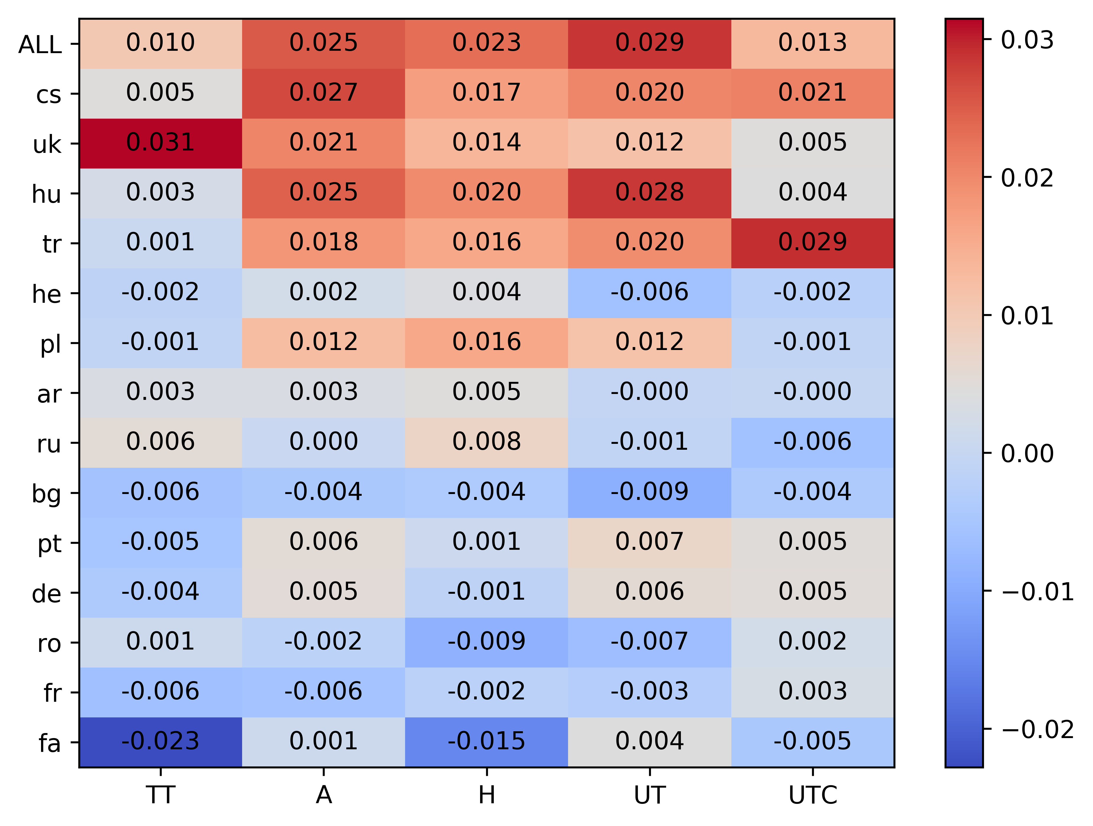
Figure 4: Feature weights of the feature-augmented language adapted linear regression model. The first row represents the “general” set of weights used for all of the languages. Each row below are the language-adapted weights that only “fire” for that specific language.

The matrix of learned weights ${\boldsymbol{\mathbf{\phi}}}$ is visualized in Figure 4. The first row of weights correspond to the “general” weights that are used for all the languages, followed by language-specific weights sorted by relative gain.

While the general weights align with the correlation results (Table 4), this analysis also shows that the UTC weight for Czech and Turkish are much larger than any of the other languages’ and indeed we can verify that these languages have $194$ and $300$ different tag combinations while the average tag combinations is $\approx 110$.

From the corpus-dependent features, word alignment score strongly predicts the gain in BLEU scores. For Czech, Ukrainian, Turkish, Hungarian, and Polish we see additional weight placed on this feature. A similar trend can be seen for the word-entropy feature. While type-token ratio does not exhibit a strong overall trend, we see that Ukrainian and Farsi are outliers.

Our correlation and regression analysis strongly suggest that CG character-aware modeling helps the most when the target language has inherent morphological complexity and that it does indeed have the ability to handle morphological patterns present in the target languages.

6.1 Qualitative Examples

Src	here he is : leonardo da vinci .
Ref	h*A hw – lywnArdw dA fyn$y .
Std	hnA hw : lywnArdw dA dA .
CG	hnA hw : lywnArdw dA fy+n$y .
Src	i ’m the mexican in the family .
Ref	AnA Almksyky fy AlEA}lp .
Std	AnA mksy+Any fy AlEA}lp .
CG	AnA Almksy+ky fy AlEA}lp .
Src	there was going to be a national referendum .
Ref	wtm AlAEdAd lAHrA’ AstftA’ $Eby .
Std	sykwn hnAk f+tA’ wTny .
CG	sykwn hnAk Ast+f+tA’ wTny .
Src	there are ordinary heroes .
Ref	fhnAk AbTAl TbyEywn .
Std	hnAk ASdqA’ EAdy .
CG	hnAk AbTAl EAdyyn .

Table 5: Examples from En-Ar, transliterated with the Buckwalter schema. We show the version of our model and the English using ‘+’ to denote where BPE splits words up, while BPE has not been applied to the target reference. author=adi,color=green,size=,fancyline,caption=,inline,]room for one or two more example?

We additionally look at specific examples of where our model is outperforming the baseline in the case of $30$k BPE in En-Ar. We see a few trends, which we show examples of in Table 5. The first trend, corresponding to the first example, is that it gets names better. This might be because Arabic is not written in the Latin alphabet, and the spelling-aware model may be able to transliterate better.

Another trend is that CG gets the endings of rare words correct, in particular when the BPE segmentation is not according to morpheme boundaries. The second example illustrates this, where the word for “Mexican” appears in the training data broken up by BPE with various morphological endings, all of which are spelled beginning with “ky” in the second subword. The morpheme boundaries here would be “Al+mksyk+y.” Note that CG also gets the definite article “Al” correct while the baseline does not.

Finally, we see a pattern where our model does better for words which are rare and appear both with and without the definite article “Al.” Our third example in Table 5 illustrates this with an infrequent word, the word for “referendum”, which gets broken up into subwords. In particular, the first subword sometimes has an “Al” attached in the training data. Our model is able to translate this subword, while the baseline skips the subword altogether, outputting two subwords that alone are not a valid word. Again, the word is not broken up along morpheme boundaries by BPE. Here there would be no way to break this word up into morphological segments—it consists of non-concatenative derivational morphology. This occurs again in the fourth example in the word for “heroes,” where the baseline predicts the word for “friends.” In this case the word was not split up by BPE, but similarly it is rare but occurs with the definite article attached in the training data as well.

7 Conclusion

We extend character-aware word-level modeling to the decoder for translation into morphologically rich languages. Our improvements were attained by augmenting the softmax and the target embedding layers with character-awareness. We also find it critical to add a gating function to balance compositional embeddings with standard embeddings. We evaluate our method on a low-resource dataset translating from English into 14 languages, and on top of a spectrum of BPE merge operations. Furthermore, for word-level and higher merge hyperparameter settings, we introduced an approximation to the softmax layer. We achieve consistent performance gains across languages and subword granularities, and perform an analysis indicating that the gains for each language correspond to morphological complexity.

For future work, we would like to explore how our methods might be of use in higher-resource settings. Furthermore, it would be interesting to see how these methods might interact with multilingual systems and if they might be able to improve what information is shared between related languages. author=pamela,color=cyan,size=,fancyline,caption=,inline,]I added a sentence to the conclusion to help us hit 8 pages and to end on a bit more of a positive note (and not the one the sassy reviewer commented on)

Appendix A More Detailed Results

In Table 6, we provide the number of training sentences for each language.

In Table 7, we provide the full experiments of our sweep of BPE for both standard and our CG embeddings. In our baseline, we see a divergence in trends across languages while sweeping over BPE merge hyperparameters—Czech (cs), Turkish (tr), and Ukrainian (uk) for example, are highly sensitive to the BPE merge hyperparameter. On the other hand, for languages like French (fr) and Farsi (fa), the performance is mostly consistent across different BPE merge hyperparameters.

author=pamela,color=cyan,size=,fancyline,caption=,inline,]Do we need to submit this separately?

Language	Number of sentences
Czech (cs)	81k
Ukrainian (uk)	74k
Hungarian (hu)	108k
Polish (pl)	149k
Hebrew (he)	181k
Turkish (tr)	137k
Arabic (ar)	168k
Portuguese (pt)	147k
Romanian (ro)	155k
Bulgarian (bg)	159k
Russian (ru)	174k
German (de)	146k
Farsi (fa)	106k
French (fr)	149k

Table 6: Number of sentences in training data for each language

L	M	Char- Shallow	Char- Deep	BPE (Subwords)						Word- Level
				1.6k	3.2k	7.5k	15k	30k	60k
cs	Std.	11.16	18.45	20.28	20.51	20.57	19.60	18.73	17.60	18.44
	CG	-	-	20.71	21.04	21.41	21.14	21.28	20.97	21.49
uk	Std.	4.77	-	13.35	15.51	15.79	15.36	14.27	12.50	12.94
	CG	-	-	13.80	16.16	15.48	16.28	16.60	15.54	15.30
hu	Std.	2.51	16.02	15.77	16.33	15.62	16.61	15.45	14.81	14.18
	CG	-	-	16.58	16.61	16.88	17.23	17.21	17.05	16.52
pl	Std.	10.65	16.31	16.14	16.40	16.34	16.76	15.98	15.47	15.49
	CG	-	-	16.88	17.12	16.84	17.63	18.00	17.32	17.20
he	Std.	22.28	23.87	23.07	23.36	23.32	22.76	22.47	21.84	21.26
	CG	-	-	23.52	23.38	23.65	23.33	23.86	22.78	23.01
tr	Std.	5.29	13.94	14.92	14.58	15.11	14.75	13.82	13.69	12.58
	CG	-	-	14.42	15.25	15.51	15.54	15.83	15.05	14.75
ar	Std.	3.58	15.89	15.66	15.67	16.22	15.70	15.05	14.86	14.45
	CG	-	-	15.96	15.55	16.17	15.99	16.28	15.53	16.05
pt	Std.	35.00	37.06	37.47	37.53	37.61	37.85	37.05	37.11	37.13
	CG	-	-	37.94	37.98	37.77	38.28	38.35	38.11	38.36
ro	Std.	21.58	22.45	23.48	24.02	23.72	23.78	22.88	22.73	22.39
	CG	-	-	23.55	23.42	23.61	24.20	24.00	23.38	23.27
bg	Std.	26.40	29.81	31.17	31.41	31.63	31.09	30.92	30.44	30.18
	CG	-	-	31.43	31.71	31.81	32.20	31.90	31.58	31.43
ru	Std.	14.63	-	18.17	18.71	19.05	18.80	19.28	18.28	17.60
	CG	-	-	18.68	19.26	19.40	19.30	19.61	19.23	19.04
de	Std.	23.89	25.93	26.98	27.34	27.37	27.23	26.94	27.21	26.84
	CG	-	-	26.94	27.55	27.46	27.89	28.12	27.37	27.75
fa	Std.	7.44	12.73	12.87	12.71	12.86	12.94	12.94	13.20	12.85
	CG	-	-	12.35	12.98	13.38	13.36	13.52	13.31	12.79
fr	Std.	32.71	34.76	35.97	35.75	35.82	35.90	35.31	35.33	35.28
	CG	-	-	35.89	35.68	36.17	36.10	35.92	36.08	36.01

Table 7: BLEU scores (case insensitive) for a standard embedding encoder-decoder baseline (Std), and character-aware model, composed embedding combined with standard embedding (CG) for $14$ languages and various BPE merge hyperparameters. For purely character-level we only train the standard model as CG would not have a sequence of characters to compose. For BPE of $60$k and word-level we use the softmax approximation described. We see that CG obtains the best result in all languages.

References

- [Bahar et al., 2017] Bahar, Parnia, Tamer Alkhouli, Jan-Thorsten Peter, Christopher Jan-Steffen Brix, and Hermann Ney. 2017. Empirical investigation of optimization algorithms in neural machine translation. The Prague Bulletin of Mathematical Linguistics, 108(1):13–25.
- [Bahdanau et al., 2015] Bahdanau, Dzmitry, Kyunghyun Cho, and Yoshua Bengio. 2015. Neural machine translation by jointly learning to align and translate. International Conference on Learning Representations.
- [Belinkov et al., 2017] Belinkov, Yonatan, Nadir Durrani, Fahim Dalvi, Hassan Sajjad, and James Glass. 2017. What do neural machine translation models learn about morphology? In Proceedings of the 55th Annual Meeting of the Association for Computational Linguistics (Volume 1: Long Papers), pages 861–872. Association for Computational Linguistics.
- [Bentz et al., 2016] Bentz, Christian, Tatyana Ruzsics, Alexander Koplenig, and Tanja Samardzic. 2016. A comparison between morphological complexity measures: typological data vs. language corpora. In Proceedings of the Workshop on Computational Linguistics for Linguistic Complexity (CL4LC), pages 142–153.
- [Cettolo et al., 2012] Cettolo, Mauro, Christian Girardi, and Marcello Federico. 2012. Wit3: Web inventory of transcribed and translated talks. In Conference of European Association for Machine Translation, pages 261–268.
- [Cherry et al., 2018] Cherry, Colin, George Foster, Ankur Bapna, Orhan Firat, and Wolfgang Macherey. 2018. Revisiting character-based neural machine translation with capacity and compression. In Proceedings of the 2018 Conference on Empirical Methods in Natural Language Processing, pages 4295–4305.
- [Chung et al., 2016] Chung, Junyoung, Kyunghyun Cho, and Yoshua Bengio. 2016. A character-level decoder without explicit segmentation for neural machine translation. In Proceedings of the 54th Annual Meeting of the Association for Computational Linguistics (Volume 1: Long Papers), pages 1693–1703.
- [Costa-jussà and Fonollosa, 2016] Costa-jussà, Marta R and José AR Fonollosa. 2016. Character-based neural machine translation. In Proceedings of the 54th Annual Meeting of the Association for Computational Linguistics (Volume 2: Short Papers), pages 357–361.
- [Daumé III, 2007] Daumé III, Hal. 2007. Frustratingly easy domain adaptation. In Proceedings of the 45th Annual Meeting of the Association of Computational Linguistics, pages 256–263, June.
- [Duh, 2018] Duh, Kevin. 2018. The multitarget ted talks task. http://www.cs.jhu.edu/~kevinduh/a/multitarget-tedtalks/.
- [Dyer et al., 2013] Dyer, Chris, Victor Chahuneau, and Noah A Smith. 2013. A simple, fast, and effective reparameterization of ibm model 2. In Proceedings of the 2013 Conference of the North American Chapter of the Association for Computational Linguistics: Human Language Technologies, pages 644–648.
- [Gage, 1994] Gage, Philip. 1994. A new algorithm for data compression. C Users J., 12(2):23–38, February.
- [Gehring et al., 2017] Gehring, Jonas, Michael Auli, David Grangier, Denis Yarats, and Yann N Dauphin. 2017. Convolutional Sequence to Sequence Learning. ArXiv e-prints, May.
- [Jean et al., 2015] Jean, Sébastien, Kyunghyun Cho, Roland Memisevic, and Yoshua Bengio. 2015. On using very large target vocabulary for neural machine translation. In Proceedings of the 53rd Annual Meeting of the Association for Computational Linguistics and the 7th International Joint Conference on Natural Language Processing (Volume 1: Long Papers), pages 1–10.
- [Kim et al., 2016] Kim, Yoon, Yacine Jernite, David Sontag, and Alexander M Rush. 2016. Character-aware neural language models. In 30th AAAI Conference on Artificial Intelligence, AAAI 2016.
- [Klein et al., 2017] Klein, Guillaume, Yoon Kim, Yuntian Deng, Jean Senellart, and Alexander M. Rush. 2017. Opennmt: Open-source toolkit for neural machine translation. In Proceedings of the 55th Annual Meeting of the Association for Computational Linguistics, ACL 2017, Vancouver, Canada, July 30 - August 4, System Demonstrations, pages 67–72.
- [Ling et al., 2015] Ling, Wang, Isabel Trancoso, Chris Dyer, and Alan W Black. 2015. Character-based neural machine translation. arXiv preprint arXiv:1511.04586.
- [Luong et al., 2015] Luong, Thang, Hieu Pham, and Christopher D. Manning. 2015. Effective approaches to attention-based neural machine translation. In Proceedings of the 2015 Conference on Empirical Methods in Natural Language Processing, EMNLP 2015, Lisbon, Portugal, September 17-21, 2015, pages 1412–1421.
- [Maruf and Haffari, 2018] Maruf, Sameen and Gholamreza Haffari. 2018. Document context neural machine translation with memory networks. In Proceedings of the 56th Annual Meeting of the Association for Computational Linguistics (Volume 1: Long Papers), volume 1, pages 1275–1284.
- [Miyamoto and Cho, 2016] Miyamoto, Yasumasa and Kyunghyun Cho. 2016. Gated word-character recurrent language model. In Proceedings of the 2016 Conference on Empirical Methods in Natural Language Processing, pages 1992–1997.
- [Och and Ney, 2003] Och, Franz Josef and Hermann Ney. 2003. A systematic comparison of various statistical alignment models. Computational linguistics, 29(1):19–51.
- [Passban et al., 2018] Passban, Peyman, Qun Liu, and Andy Way. 2018. Improving character-based decoding using target-side morphological information for neural machine translation. In Proceedings of the 2018 Conference of the North American Chapter of the Association for Computational Linguistics: Human Language Technologies, Volume 1 (Long Papers), volume 1, pages 58–68.
- [Sennrich et al., 2016] Sennrich, Rico, Barry Haddow, and Alexandra Birch. 2016. Neural machine translation of rare words with subword units. In Proceedings of the 54th Annual Meeting of the Association for Computational Linguistics, ACL 2016, August 7-12, 2016, Berlin, Germany, Volume 1: Long Papers.
- [Shapiro and Duh, 2018] Shapiro, Pamela and Kevin Duh. 2018. Bpe and charcnns for translation of morphology: A cross-lingual comparison and analysis. arXiv preprint arXiv:1809.01301.
- [Sylak-Glassman et al., 2015] Sylak-Glassman, John, Christo Kirov, Matt Post, Roger Que, and David Yarowsky. 2015. A universal feature schema for rich morphological annotation and fine-grained cross-lingual part-of-speech tagging. In International Workshop on Systems and Frameworks for Computational Morphology, pages 72–93. Springer.