Inner-shell clock transition in atomic thulium with small BBR shift
Abstract
With direct polarizability measurements we demonstrated extremely low sensitivity of the inner-shell clock transition at m in Tm atoms to external dc electric fields and black-body radiation (BBR). We measured differential polarizabilities of clock levels in Tm at wavelengths of 810–860 nm and at 1064 nm and inferred the static scalar differential polarizability of the inner-shell clock transition of atomic units corresponding to only fractional frequency shift from BBR at the room temperature. This is a few orders of magnitude smaller compared to the BBR shift of the clock transitions in the neutral atoms (Sr, Yb, Hg) and competes with the least sensitive ion species (e.g. Al+ or Lu+). For the m clock transition, we experimentally determined the “magic” wavelength of nm, recorded the transition spectral linewidth of Hz, and measured its absolute frequency of Hz.
pacs:
Unprecedented performance of the state-of-the-art optical atomic clocks Chen2017 ; Ushijima2015 ; Marti2018 together with the increasing number of characterized clock transitions in different atomic and ionic species opened new frontiers in physics, namely, sensitive tests of special relativity Delva2017 ; Shaniv2018 , search for dark matter roberts2017search ; Wciso2018 and variations of fundamental constants Rosenband2008 ; Borkowski2018 , atom-based quantum simulations Norcia259 , and some other as summarized in reviews Ludlow2015 ; Poli2014 ; safronova2018search . Moreover, development of robust, compact, and transportable optical clocks Koller2017 overcoming in accuracy the best microwave frequency standards promises a new era in precision spectroscopy, navigation, and geodesy Grotti2018 ; takano2016geopotential .
The fractional frequency instability of optical clocks reaching low level was successfully demonstrated for Sr Nicholson2015 and Yb schioppo2017ultrastable optical lattice clocks as well as for Yb+ Huntemann2016 and Al+ Chou2010 single-ion optical clocks. One of the current limitations is the impact of electric fields like surrounding black body radiation (BBR), trapping fields, and collisions. To push forward the current limit in frequency stability and accuracy, there is a continuous search for new species, particularly with the reduced sensitivity to external electric fields. Among promising candidates are single Lu+ ion Arnold2018 , highly charged ions nauta2017towards ; Yu2018 ; Kozlov2018 , and 229Th with an isomeric nuclear transition Wense2017 ; thielking2018laser .
Lanthanides with the submerged electronic -shell possess natural suppression of the sensitivity to external electric fields for the inner-shell - transitions because of strong shielding by the closed and shells. Already in 1984, E. Alexandrov and co-authors demonstrated unusually low spectral broadening of the 1.14 m inner-shell transition in atomic Tm under collisions with buffer He gas aleksandrov1984eb . In 2004, strong shielding effect for Tm-He collisions was confirmed in ref. Hancox2004 . Similar effect was also observed for some transition elements with nonzero orbital angular momentum Hancox2005 . For lanthanide ions doped in solids, the shielding effect reduces inhomogeneous broadening of the inner-shell - transitions which allows, for example, ensemble-based solid-state quantum memory probst2013 and integrated single-photon source in telecom wavelength range Dibos2018 . However, the possibility to use such transitions for optical clocks was studied only theoretically Kozlov2013 ; kozlov2014optical ; Sukachev2016 .
In this Letter, we report on precision spectroscopy of the inner-shell clock transition between the fine-structure components of the ground electronic state in atomic Tm at the wavelength of 1.14 m with the natural linewidth of Hz (here and stand for the electronic and total momentum quantum numbers, respectively, and is the magnetic quantum number). Spectroscopy of the clock transition leads to zero first order Zeeman and magnetic dipole-dipole interaction shifts Sukachev2016 . We experimentally determined magic wavelength of the optical lattice near 813 nm, recorded Fourier-limited spectral linewidth of the clock transition of 10 Hz and characterized its sensitivity to electric and magnetic fields. Accurate measurement of differential dynamic polarizabilities of the clock levels in the near infrared spectral region (810–860 nm and 1064 nm) allowed to estimate the BBR frequency shift of the clock transition, which turned out to be a few orders of magnitude smaller compared to other characterized clock transitions in neutral atoms.
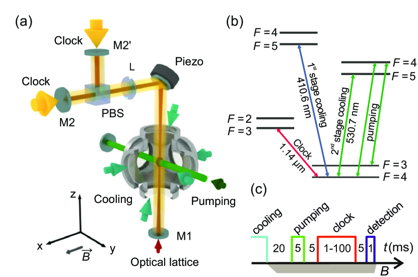
Thulium atoms are laser cooled in a two-stage magneto-optical trap (see Fig. 1 and detailed description in ref. sukachev2014secondary ). For precision spectroscopy, atoms at a temperature of K are loaded in a vertical optical lattice formed inside an enhancement cavity (finesse equals 20) with intra-cavity polarization filtering. The cavity allows to build-up optical power from a 1 W Ti:sapphire laser up to 6 W in the wavelength range of 810–860 nm. The beam waist radius can be varied between 80 m and 160 m by controlling the distance between cavity elements.
We prepare atoms in lower clock state by driving simultaneously (pump) and (repump) transitions with a 5 ms-long -polarized laser pulses at 530.7 nm in the presence of a bias magnetic field of G. After the optical pumping cycle, atoms are trapped in the lattice with more than 80% in the target state. To interrogate the clock transition, we use radiation of a semiconductor m laser stabilized to a high-finesse Ultra Low Expansion glass (ULE) cavity, providing the relative frequency instability of smaller than 10-14 in 1-100 s integration time Alnis2008 . The linear frequency drift of 29 mHz/s is compensated using an acousto-optical modulator. After compensation, the clock laser can be used as a stable frequency reference for studying frequency shifts of the clock transition.
Results
Magic wavelength determination. The important step towards high resolution spectroscopy of the clock transition is determination of a magic wavelength of the optical lattice when dynamic polarizabilitites of the clock levels become equal Takamoto2003 . We numerically calculated dynamic polarizabilities of the clock levels using time-dependent second order perturbation theory and transition data obtained using COWAN package cowan1981 (Model 1 described in Methods and in ref. Sukachev2016 ), and predicted existence of the magic wavelength at 811.2 nm (for the collinear magnetic field and the lattice field polarization ) near a narrow transition from the upper clock level at nm. Calculated differential polarizability is shown in Fig. 2 with the red solid line. This wavelength region is readily accessible by Ti:sapphire or powerful semiconductor lasers.
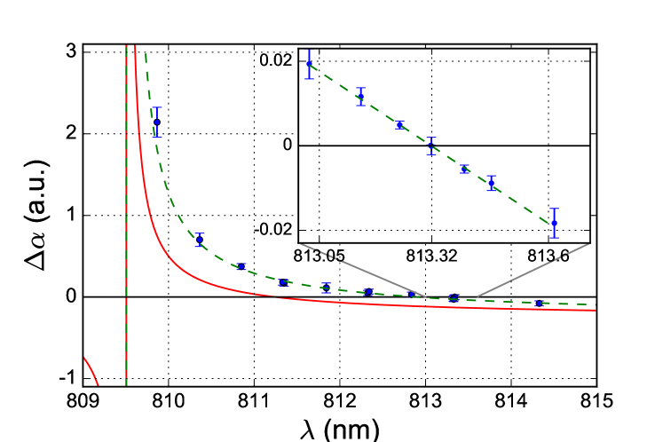
Using an approach described in ref. Barber2008 , we experimentally searched for the magic wavelength for the clock transition in the spectral region of 810–815 nm. The transition frequency shift as a function of optical lattice power was measured at different lattice wavelengths. The differential dynamic polarizability between the clock levels was calculated using the expression . Here is the Plank constant, is the speed of light, is the Bohr radius, and m is the lattice beam radius which was calculated from the enhancement cavity geometry. The intra-cavity power was determined by calibrated photodiodes placed after the cavity outcouplers M2 and M2′. The details of the beam waist determination and power measurements are given in Methods. Figure 2 shows the spectral dependency of in atomic units (a.u.). The magic wavelength of nm was determined by zero crossing of the linear fit in the inset of Fig. 2.
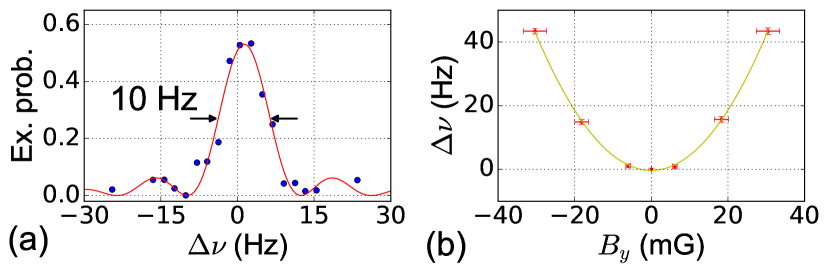
Trapping Tm atoms in the optical lattice at drastically reduces inhomogeneous ac Stark broadening of the clock transition. Exciting with a 80 ms-long Rabi pulses of the clock laser we recorded a spectrum with 10 Hz full width at the half maximum shown in Fig. 3(a). Non-unity excitation at the line center comes from a non-perfect initial polarization of atoms and finite lifetime of the upper clock level ( ms).
Using Ti:sapphire frequency comb, we determined the absolute frequency of clock transition in Tm of Hz. The relative frequency uncertainty of mainly comes from instability and calibration accuracy of a GLONASS-calibrated passive hydrogen maser used as a frequency reference for the comb.
Differential polarizability analysis. In the second order approximation, the energy shift of an atomic level in an external oscillating electromagnetic field with the wavelength equals , where is the amplitude of the electric field. For linear field polarization, the dynamic polarizability can be split in the scalar and the tensor parts as:
| (1) |
where is the angle between the quantization axis (here the direction of the external magnetic field ) and the electric field polarization of the optical lattice. In our case, the differential polarizability of the two clock levels equals
| (2) |
where and . By definition, at the magic wavelength the differential polarizability vanishes: .
The frequency shift of the clock transition due to the optical lattice can be caused by (i) accuracy of the magic wavelength determination and (ii) angular dependency of the tensor part of the differential polarizability. The accuracy of the magic wavelength determination is related to the slope of in the vicinity of , which is a.u/nm for nm in Tm, as it is shown in the inset in Fig. 2. In more practical units, this corresponds to the clock transition frequency shift of mHz for lattice frequency detuning [GHz] from and lattice depth in units of the recoil energy. This value is more than one order of magnitude smaller compared to the corresponding sensitivity of Sr and Yb lattice clocks Barber2008 ; brown2017hyperpolarizability .
For , the differential tensor polarizability influences the clock transition frequency as:
| (3) |
To find , we measured dependency of the clock transition frequency shift on a small magnetic field at the constant bias fields mG and () shown in Fig. 3(b). From the corresponding parabolic coefficient of 56(11) mHz/mG2, we get the differential tensor polarizability of a.u. at . The uncertainty comes from the absolute calibration of magnetic field and power calibration (see Methods). Both lattice frequency shifts mentioned in the previous paragraph can be readily reduced to mHz level by stabilizing the lattice wavelength with 0.1 GHz accuracy and by maintaining .
The frequency of clock transition possesses a quadratic sensitivity to a dc magnetic field with a coefficient Hz/G2 Sukachev2016 . To provide uncertainty of the transition frequency below 1 mHz, it would be necessary to stabilize magnetic field at the level of G at the bias field of mG. Note, that the quadratic Zeeman shift in Tm can be fully canceled by measuring an averaged frequency of two clock transitions and [Fig. 1(b)] possessing the quadratic Zeeman coefficients of the opposite signs. To implement this approach, one should provide the magic-wavelength condition for both transitions. This can be done by choosing to cancel the tensor part in Eq. (2) and tuning the lattice wavelength approximately to 850 nm [Fig. 4(b)]. At this wavelength the differential scalar polarizability vanishes for both transitions ( since ).
Static differential polarizability and the BBR shift. The BBR shift of the clock transition frequency can be accurately calculated from the static differential scalar polarizability from a theoretical model based on the measured polarizability spectrum at the wavelengths of 810–860 nm and at 1064 nm.
Measurements in the spectral region of 810–860 nm were done by scanning the wavelength of the Ti:sapphire laser at two polarizations corresponding to () and () as shown in Fig. 4(a). The corresponding scalar and tensor differential polarizabilities calculated from Eq. (2) are shown in Fig. 4(b).
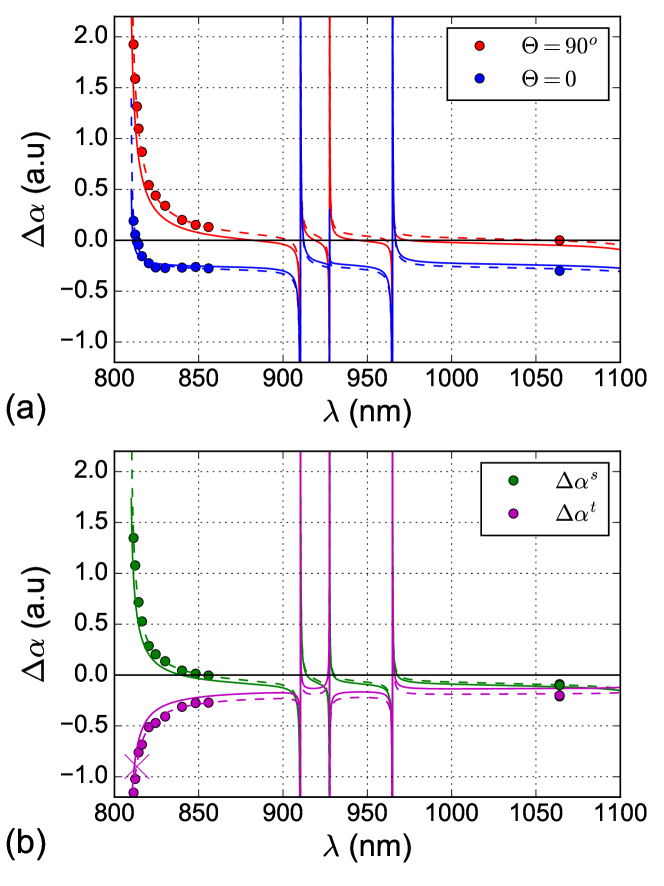
To measure dynamic polarizability at 1064 nm, we used a slightly different procedure: Tm atoms were trapped in the optical lattice at for which the differential polarizability vanishes, and the atomic cloud was illuminated along -axis by a focused beam of a linearly-polarized single-frequency 1064 nm fiber laser with the optical power up to 10 W. Corresponding results for () and () are also shown in Fig. 4.
To compare with experimental data and to deduce , we use Model 2 (see Methods), which differs from Model 1 by introducing four adjustable parameters: probabilities of the 806.7 nm and 809.5 nm transitions and two offsets for differential scalar and tensor polarizabilities. Corresponding fits based on Model 2 are shown as dashed lines in Fig. 4, while calculations with no free parameters (Model 1) are shown as solid lines. From Model 2 we obtain
| (4) |
The differential static scalar polarizability from Model 1 is a.u., which differs by only 1 standard deviation from (4). Calculations of the BBR frequency shift can be readily done using the value of Sukachev2016 . The differential scalar polarizability in the spectral region around m (the maximum of the BBR spectrum at the room temperature) differs by less than a.u. from . Note, that there are no resonance transitions from the clock levels for m. For our clock transition at m the room temperature BBR shift is mHz. It is a few orders of magnitude smaller than for other neutral atoms and is comparable to the best ions species as shown in Table 1. This result quantitatively confirms the idea of strong shielding of inner-shell transitions in lanthanides from external electric fields.
The clock transition frequency shifts due to a magnetic component of the BBR and electric field gradient of the optical lattice are less than Hz and can be neglected (see Methods).
| Element | ||
|---|---|---|
| Tm (this work) | ||
| Sr 111ref. Ludlow2015 | ||
| Yb 11footnotemark: 1 | ||
| Hg 222ref. Bilicki2016 | ||
| Yb+ (E3)11footnotemark: 1 | ||
| Al+ 11footnotemark: 1 | ||
| Lu+ 333transition , ref. Arnold2018 |
Discussion
Specific shielding of the inner-shell magnetic-dipole clock transition in atomic thulium at 1.14 m by outer 5 and 6 electronic shells results in a very low sensitivity of its frequency to external electric fields. The differential static scalar polarizability of the two and clock levels is only atomic units which corresponds to the fractional BBR frequency shift of the transition of at the room temperature. It is by three orders of magnitude less compared to the prominent clock transitions in Sr and Yb (see Table 1). Taking into account that all major frequency shifts (the Zeeman shift, lattice shifts, collisional shifts) can be controlled at the low level, these features make thulium a promising candidate for a transportable room-temperature optical atomic clock due to soft constrains on the ambient temperature stability. It combines advantages of unprecedented frequency stability of optical lattice clocks on neutral atoms and low sensitivity to BBR of ion optical clocks. Moreover, precision spectroscopy in Tm opens possibilities for sensitive tests of Lorentz invariance Shaniv2018 and for search of the fine structure constant variation kolachevsky2008high .
Optical clocks based on a - transition in some other lanthanides with spinless nuclei could be even more attractive featuring the low sensitivity to magnetic fields due to the absence of the hyperfine structure and small BBR shift. For example, the fine-structure clock transition at the telecom-wavelength of 1.44 m in laser-cooled erbium atoms (e.g. 166Er) McClelland2006 ; Kozlov2013 can be particularly interesting for optical frequency dissemination over fiber networks Riehle2017 .
Methods
Enhancement cavity. Optical lattice is formed inside a -shaped enhancement cavity, as shown in Fig. 1(a). The reflectivity of the curved (the radius is mm) incoupler mirror M1 equals 87% and matches losses introduced by the vacuum chamber viewports. Outcouplers M2 or M2′ are identical flat mirrors with the reflectivity of . For locking to the laser frequency, the cavity mirror reflecting the beam at is mounted on a piezo actuator. The intra-cavity polarization is defined by a broadband polarization beam splitter; depending on the polarization, either M2 or M2′ outcoupler mirror is used. The intra-cavity lens has the focal length of mm.
Depending on experimental geometry ( or ), we couple corresponding linearly polarized radiation from the Ti:sapphire laser through the incoupler mirror M1. Intra-cavity polarization filtering by PBS defines the polarization angle and significantly improves polarization purity of the optical lattice. The angle between the laser field polarization and the bias magnetic field is adjusted with the accuracy of better than .
Measurement of differential dynamic polarizabilities. Differential polarizability of the clock levels is determined from the frequency shift of the corresponding transition , circulating power , and TEM00 cavity mode radius at the atomic cloud position as
| (5) |
The dependency was obtained for different wavelengths in the spectral range 810–860 nm for the intra-cavity circulating power varying from 1 W to 4 W, as it is shown in Fig. 5. Frequency shifts were measured relative to the laser frequency, which is stabilized to an ultra-stable ULE cavity with linear drift compensation. The slope coefficients of corresponding linear fits were substituted to Eq. (5) to deduce presented in Figs. 2, 4.
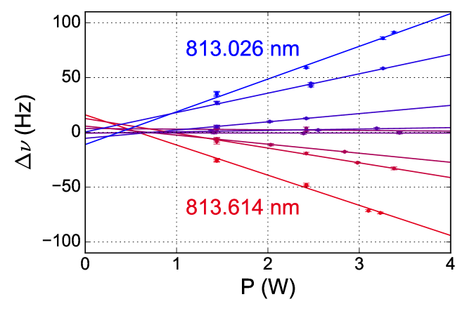
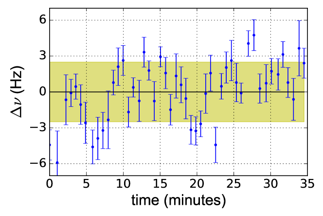
Uncertainty of the frequency shift comes from the residual instability of the reference cavity on time intervals of 1000 s. To estimate it, we measured clock transition frequency relative to the clock laser frequency at the magic wavelength when the perturbations from the lattice are minimal. Results are shown in Fig. 6. The standard deviation equals to 2.6 Hz contributing a.u. to the error budget of . For the lattice wavelength detuned from contribution of the laser frequency instability is negligible.
The intra-cavity power was determined by measuring power leaking through the cavity outcoupler M2 (or M2′) using calibrated photodiodes. For each photodiode we measured the power-to-voltage transfer function , where is the voltage reading from the photodiode, and is the coefficient measured using absolutely calibrated Thorlabs S121C power meter. To determine , we unlocked the cavity, slightly tilted the outcoupler, blocked the reflected beam to prevent feasible reflections from the incoupler, and measured the power before the outcoupler and corresponding voltage reading of the photodiode. The linearity of the photodiode response was checked separately and turned out to be better than in the working region. The photodiode calibration was done in the whole spectral range of 810–860 nm to take into account the spectral response of the outcoupler and the photodiode. Although the specified uncertainty of the power sensor Thorlabs S121C equals 3%, we ascribe the net uncertainty of power measurement of 10% from comparison of readings from three different absolutely calibrated sensors.
The beam radius at the atomic cloud position is deduced from the cavity geometry: distances from the vacuum chamber center (and target atomic cloud position) to M1, L and M2 (or M2′) are 244 mm, 384 mm and 500 mm, respectively, giving the beam radius of m at the position of atomic cloud. The uncertainty of comes from the position uncertainties of cavity elements and of the atomic cloud with respect to the chamber center, as well as from uncertainty of 1 mm of the lens focal length. We conservatively evaluate position uncertainties of M1, L, and M2 (or PBS and M2′) as 1 mm, and the possible axial displacement of the atomic cloud of 2 mm. The partial contributions to the beam radius uncertainty are m (the incoupler), m (the lens), m (the outcoupler), m (the cloud) and m (focal length). Adding up in quadratures, the total uncertainty of the beam radius equals m. The result is independently confirmed by measuring frequency intervals between cavity transversal modes.
The finite temperature of the atomic cloud reduces averaged light intensity on the atomic cloud in respect to the on-axis antinode lattice intensity . Assuming Boltzman distribution of the atoms with the temperature in the trap of depth one can calculate the parameter connecting the averaged and maximum intensity . The parameter is calculated from
| (6) |
where is the classical turning point. The parameter equals for (which corresponds to average experimental conditions). One standard deviation of corresponds to range from to , while already covers ( - range.
Summarizing, we evaluate the uncertainty of measured differential polarizability to be 13% with the dominating contribution from power calibration. In the vicinity of , the uncertainty is slightly higher by 0.003 a.u. because of the reference clock laser frequency instability.
To measure differential polarizability at 1064 nm, atoms were trapped in the optical lattice at the magic wavelength and irradiated by focused slightly elliptic 1064 nm laser beam with the waists of m and m in and directions, respectively. To adjust the 1064 nm laser beam center to the atomic cloud, we maximized intensity of the beam on the atomic cloud by monitoring the frequency shift of the clock transition. To increase sensitivity, corresponding measurements were done by tuning the clock laser to the slope of 1.14 m transition.
For the measurement session of at , we performed three adjustments of 1064 nm laser beam. The reproducibility corresponds to the frequency shift of 5 Hz at the maximal frequency shift of 25 Hz. The resulting linear coefficient is evaluated as Hz/W including this uncertainty. In configuration, we did not observe any significant effect from adjustment and the coefficient equals Hz/W.
Theoretical analysis. Theoretical approach to calculate polarizabilities of Tm atomic levels is described in our previous works Sukachev2016 ; golovizin2017methods . Calculations are based on the time-dependent second order perturbation theory with summation over known discrete transitions from the levels of interest. For calculations, we used transitions wavelengths and probabilities obtained with the COWAN package cowan1981 with some exceptions: for transitions with nm, experimental wavelengths from ref. NIST_ASD are used. This approach allows to increase accuracy of the magic wavelength prediction in the corresponding spectral region of nm. According to calculations, the magic wavelength was expected at 811.2 nm which motivated our experimental studies in the spectral region 810–815 nm (see Fig. 2). We refer to this model as “Model 1” and use for comparison with experimental results of this work as shown in Figs. 2,4.
Deviation of the experimental data from Model 1 can be explained by two main factors. First, in this model we did not take into account transitions to the continuum. Together with uncertainties of COWAN calculations of transition amplitudes, it can result in a small offset of the infrared differential polarizability spectrum. Note, that although transitions to the continuum spectrum may significantly contribute to polarizabilities of the individual levels (up to 10%), for the differential polarizability of the - transition at 1.14 m in Tm contribution of the continuum is mostly canceled Sukachev2016 .
| Source | Uncertainty, a.u. |
|---|---|
| Experimental results for 810–850 nm | |
| Experimental result for nm | |
| Angle | |
| Transition probabilities for nm | |
| Total | |
| For the reference: | |
| Difference of Models 1 and 2 |
To fit experimental data we use Model 2 which differs from Model 1 by introducing four fit parameters. As parameters we use the probabilities of the 806.7 nm and 809.5 nm transitions which mostly effect polarizability spectrum in 810–860 nm region and two offsets for the scalar and tensor polarizabilities. After fitting the experimental data (see Fig. 4) by Model 2, the probability of the 806.7 nm transition is changed from to , the probability of the 809.5 nm transition is changed from 149 s-1 to 357(109) s-1, the fitted offsets for the differential scalar and tensor polarizabilities equal a.u. and a.u. with reduced for the fits of 1.35 and 2.9, respectively.
Transitions from the upper Tm clock level in the spectral range nm are weak and their probabilities are experimentally not measured. To calculate probabilities we used COWAN package. To estimate the impact of insufficient knowledge of transition probabilities on differential scalar polarizability , we assume possible variation of each transition probability by a factor of 2. After extrapolation of the fitted Model 2 to we get the static differential polarizability a.u., where uncertainty comes from variation of nm transition probabilities.
We summarize all sources of uncertainties which contribute to the error of the static differential polarizability in Table 2. As discussed above, the experimental uncertainty for 810–860 nm range is 13% contributing a.u. to the , while the measurement at 1064 nm is less accurate (20%) due to the laser beam adjustment and results in a.u. variation of Model 2 extrapolation. The uncertainty of the angle adjustment contributes a.u. The uncertainty coming from the poorly known transition probabilities from clock level in nm range contributes a.u. Using extrapolation of Model 2 and adding all uncertainties we come to the final result of a.u. Note, that this is fully consistent with the extrapolated value of -0.062 a.u. obtained from Model 1 and given for the reference in Table 2.
BBR magnetic field. To estimate the clock transition frequency shift due to the magnetic component of BBR, we follow the analysis given in the work gan2018oscillating . The corresponding frequency shift of one of the clock levels coupled to another atomic level with magnetic-dipole transition at frequency can be found by integrating over the full BBR spectrum as
| (7) |
where is the vacuum permittivity, K, . Here
| (8) | |||
| (9) |
The hyperfine transition frequency of the ground level in Tm equals MHz, while for the clock level it equals MHz. For these values of , , and the shift is on the order of Hz. To estimate the contribution from the optical transitions, we evaluate the shift from the lowest frequency magnetic-dipole transition at THz, which is the clock transition itself: , and Hz for the ground level (for the upper clock level the corresponding shift is Hz). Hence, we estimate total shift of the clock transition from the magnetic component of BBR to be less than Hz.
Electric quadrupole shift. Opposite to neutral Sr, Yb, and Hg atoms, Tm clock levels posses a non-zero electric quadrupole moment on the order of 1 a.u. Sukachev2016 and are coupled to an electric field gradient. Since the electric field gradient in an optical lattice oscillates at the optical frequency, the corresponding time-averaged frequency shift of the clock transition is zero.
References
References
- (1) Chen, J. et al. Sympathetic ground state cooling and time-dilation shifts in an 27Al+ optical clock. Phys. Rev. Lett. 118, 053002 (2017).
- (2) Ushijima, I., Takamoto, M., Das, M., Ohkubo, T. & Katori, H. Cryogenic optical lattice clocks. Nature Photonics 9, 185–189 (2015).
- (3) Marti, G. E. et al. Imaging optical frequencies with precision and resolution. Phys. Rev. Lett. 120, 103201 (2018).
- (4) Delva, P. et al. Test of special relativity using a fiber network of optical clocks. Phys. Rev. Lett. 118, 221102 (2017).
- (5) Shaniv, R. et al. New methods for testing lorentz invariance with atomic systems. Phys. Rev. Lett. 120, 103202 (2018).
- (6) Roberts, B. M. et al. Search for domain wall dark matter with atomic clocks on board global positioning system satellites. Nature Communications 8, 1195 (2017).
- (7) Wcisło, P. et al. First observation with global network of optical atomic clocks aimed for a dark matter detection. arXiv preprint arXiv:1806.04762 (2018).
- (8) Rosenband, T. et al. Frequency ratio of Al+ and Hg+ single-ion optical clocks; metrology at the 17th decimal place. Science 319, 1808–1812 (2008).
- (9) Borkowski, M. Optical lattice clocks with weakly bound molecules. Phys. Rev. Lett. 120, 083202 (2018).
- (10) Norcia, M. A., et al. Cavity-mediated collective spin-exchange interactions in a strontium superradiant laser. Science 361, 259–262 (2018).
- (11) Ludlow, A., Boyd, M., Ye, J., Peik, E. & Schmidt, P. Optical atomic clocks. Reviews of Modern Physics 87, 637 (2015).
- (12) Poli, N., Oates, C. W., Gill, P. & Tino, G. M. Optical atomic clocks. arXiv preprint arXiv:1401.2378 (2014).
- (13) Safronova, M. S. et al. Search for new physics with atoms and molecules. Rev. Mod. Phys. 90, 025008 (2018).
- (14) Koller, S. B. et al. Transportable optical lattice clock with uncertainty. Phys. Rev. Lett. 118, 073601 (2017).
- (15) Grotti, J. et al. Geodesy and metrology with a transportable optical clock. Nature Physics 14, 437–441 (2018).
- (16) Takano, T. et al. Geopotential measurements with synchronously linked optical lattice clocks. Nature Photonics 10, 662–666 (2016).
- (17) Nicholson, T. et al. Systematic evaluation of an atomic clock at total uncertainty. Nature communications 6, 6896 (2015).
- (18) Schioppo, M. et al. Ultrastable optical clock with two cold-atom ensembles. Nature Photonics 11, 48–52 (2017).
- (19) Huntemann, N., Sanner, C., Lipphardt, B., Tamm, C. & Peik, E. Single-ion atomic clock with systematic uncertainty. Phys. Rev. Lett. 116, 063001 (2016).
- (20) Chou, C., Hume, D., Koelemeij, J., Wineland, D. & Rosenband, T. Frequency comparison of two high-accuracy Al+ optical clocks. Phys. Rev. Lett. 104, 070802 (2010).
- (21) Arnold, K. J., Kaewuam, R., Roy, A., Tan, T. R., & Barrett, M. D. Blackbody radiation shift assessment for a lutetium ion clock. Nature Communications 9, 1650 (2018).
- (22) Nauta, J. et al. Towards precision measurements on highly charged ions using a high harmonic generation frequency comb. Nuclear Instruments and Methods in Physics Research Section B: Beam Interactions with Materials and Atoms 408, 285–288 (2017).
- (23) Yu, Y.-m. & Sahoo, B. K. Selected highly charged ions as prospective candidates for optical clocks with quality factors larger than . Phys. Rev. A 97, 041403 (2018).
- (24) Kozlov, M. G., Safronova, M. S., López-Urrutia, J. R. C. & Schmidt, P. O. Highly charged ions: optical clocks and applications in fundamental physics. arXiv preprint arXiv:1803.06532 (2018).
- (25) Wense, L. V. D. et al. A laser excitation scheme for Th. Phys. Rev. Lett. 119, 132503 (2017).
- (26) Thielking, J. et al. Laser spectroscopic characterization of the nuclear-clock isomer Th. Nature 556, 321–325 (2018).
- (27) Aleksandrov, E. B., Vedenin, V. D. & Kulyasov, V. N. Broadening and shift of thulium resonance lines by helium. Opt. Spectrosc. 56, 365–368 (1984).
- (28) Hancox, C. I., Doret, S. C., Hummon, M. T., Luo, L. & Doyle, J. M. Magnetic trapping of rare-earth atoms at millikelvin temperatures. Nature 431, 281–284 (2004).
- (29) Hancox, C. I., Doret, S. C., Hummon, M. T., Krems, R. V. & Doyle, J. M. Suppression of angular momentum transfer in cold collisions of transition metal atoms in ground states with nonzero orbital angular momentum. Phys. Rev. Lett. 94, 013201 (2005).
- (30) Probst, S. et al. Anisotropic rare-earth spin ensemble strongly coupled to a superconducting resonator. Phys. Rev. Lett. 110, 157001 (2013).
- (31) Dibos, A. M., Raha, M., Phenicie, C. M. & Thompson, J. D. Atomic source of single photons in the telecom band. Phys. Rev. Lett. 120, 243601 (2018).
- (32) Kozlov, A., Dzuba, V. A. & Flambaum, V. V. Prospects of building optical atomic clocks using Er i or Er iii. Phys. Rev. A 88, 032509 (2013).
- (33) Kozlov, A., Dzuba, V. A. & Flambaum, V. V. Optical atomic clocks with suppressed blackbody-radiation shift. Phys. Rev. A 90, 042505 (2014).
- (34) Sukachev, D. et al. Inner-shell magnetic dipole transition in Tm atoms: A candidate for optical lattice clocks. Phys. Rev. A 94, 022512 (2016).
- (35) Sukachev, D. D. et al. Secondary laser cooling and capturing of thulium atoms in traps. Quantum Electronics 44, 515–520 (2014).
- (36) Alnis, J., Matveev, A., Kolachevsky, N., Udem, T. & Hänsch, T. W. Subhertz linewidth diode lasers by stabilization to vibrationally and thermally compensated ultralow-expansion glass Fabry-Pérot cavities. Phys. Rev. A 77, 053809 (2008).
- (37) Takamoto, M. & Katori, H. Spectroscopy of the clock transition of 87Sr in an optical lattice. Phys. Rev. Lett. 91, 223001 (2003).
- (38) Cowan, R. The theory of atomic structure and spectra. (University of California Press, Berkeley, CA, 1981), and Cowan programs RCN, RCN2,and RCG.
- (39) Barber, Z. W. et al. Optical lattice induced light shifts in an Yb atomic clock. Phys. Rev. Lett. 100, 103002 (2008).
- (40) Brown, R. C. et al. Hyperpolarizability and operational magic wavelength in an optical lattice clock. Phys. Rev. Lett. 119, 253001 (2017).
- (41) Kolachevsky, N. N. High-precision laser spectroscopy of cold atoms and the search for the drift of the fine structure constant. Physics-Uspekhi 51, 1180–1190 (2008).
- (42) McClelland, J. J. & Hanssen, J. L. Laser cooling without repumping: A magneto-optical trap for erbium atoms. Phys. Rev. Lett. 96, 143005 (2006).
- (43) Riehle, F. Optical clock networks. Nature Photonics 11, 25–31 (2017).
- (44) Golovizin, A. et al. Methods for determining the polarisability of the fine structure levels in the ground state of the thulium atom. Quantum Electronics 47, 479–483 (2017).
- (45) Kramida, A., Ralchenko, Yu., Reader, J., and NIST ASD Team. NIST Atomic Spectra Database (ver. 5.5.6), [Online]. Available: https://physics.nist.gov/asd [2018, August 21]. National Institute of Standards and Technology, Gaithersburg, MD., 2018.
- (46) Gan, H. et al. Oscillating magnetic field effects in high precision metrology. arXiv preprint arXiv:1807.00424 (2018).
- (47) Tyumenev, R. et al. Comparing a mercury optical lattice clock with microwave and optical frequency standards. New Journal of Physics 18, 113002 (2016).
Acknowledgment
The work is supported by RFBR Grants No. 18-02-00628 and No. 16-29-11723. We are grateful to S. Kanorski and V. Belyaev for invaluable technical support and to S. Fedorov for assembling the frequency comb. We also thank M. Barrett for very useful discussions.
Author contributions
A.G., E.F., and D.T. carried out all measurements and analyzed the data; A.G. and D.S. did theoretical calculations; A.G., D.S., and N.K. wrote the paper. K.K., V.S., and N.K. conceived and directed the project. All authors discussed the results and commented on the manuscript.
Additional information
Competing interests: The authors declare no competing interests.