Bootstrap approach to geometrical four-point functions
in the two-dimensional critical $Q$-state Potts model:
A study of the $s$-channel spectra

Abstract

We revisit in this paper the problem of connectivity correlations in the Fortuin-Kasteleyn cluster representation of the two-dimensional $Q$-state Potts model conformal field theory. In a recent work [1], results for the four-point functions were obtained, based on the bootstrap approach, combined with simple conjectures for the spectra in the different fusion channels. In this paper, we test these conjectures using lattice algebraic considerations combined with extensive numerical studies of correlations on infinite cylinders. We find that the spectra in the scaling limit are much richer than those proposed in [1]: they involve in particular fields with conformal weight $h_{r,s}$ where $r$ is dense on the real axis.

1 Introduction

In a very interesting recent paper [1], a proposal was put forward for some of the four-point correlation functions of the percolation problem in two dimensions. This proposal was part of a more general conjecture addressing various geometrical objects involving four points in the diagrammatic formulation [2] of the $Q$-state Potts model [3]. The case $Q=1$ corresponds to percolation, and the proposal in [1] covers such objects as the probability that two of these points belong to one cluster, and the two others to another cluster. Obtaining closed-form expressions for such objects is one of the holy grails in the field. It is a far from obvious endeavour because the conformal field theory (CFT) describing percolation (and more generally geometrical features of the $Q$-state Potts model) is not well understood: it is non-unitary, probably involves logarithms (even for $Q$ generic), and involves operators which are not degenerate, precluding the use of the differential equations approach à la BPZ [4].

The construction in [1] is elegant and powerful. It starts with a seemingly reasonable hypothesis for the spectrum of operators appearing in the fusion channels for the fusion of two order operators, and determines, using a clever code, the whole set of structure constants based on our knowledge of conformal blocks [5, 6] together with the imposition of crossing symmetry. The results are then checked against Monte Carlo simulations, with, it is claimed, reasonably good agreement.

Although the results in [1] are appealing, they are not really consistent with what is known about the Potts model CFT and, in particular, percolation. Early work [7] has revealed indeed a much richer spectrum than the one postulated in [1], which covers only a very tiny set of the known full operator content of the theory. Of course, it could be that by some accident, the order operator in the $Q$-state Potts model does not couple to as many fields as one would expect, at least in the scaling limit. But it could also be that something is simply missing in the work of [1], despite the apparent numerical effectiveness of their proposal.

To investigate this question requires a long and detailed analysis, of which we present the results here. In a nutshell, we have gathered direct, in our opinion unquestionable evidence that the spectrum of the $Q$-state Potts model is as complex as could have been feared, that many more fields appear in the OPE of order operators in the Potts model than was conjectured in [1], and that the proposal in that paper, appealing as it may be, simply cannot be correct. It is, at best, a good numerical approximation to the true expressions for the four-point functions.

Our paper is organised as follows. In section 2 we remind the reader of basic facts and results about the $Q$-state Potts model and its geometrical formulation. Algebraic aspects—which constitute a crucial part of our approach—are discussed in section 3. Section 4 summarises our method of analysis, and how we extract exponents as well as amplitudes, from lattice data. Section 5 discusses our results for the spectra in the intermediate channels of four-point functions. A comparison with results in [1] is provided in section 6. In section 7, we return to the issue of divergences in the amplitudes, and re-analyse briefly our results as well as those of [1] from the point of view of degeneracies, and, potentially, logarithmic CFTs.

Since a good part of our analysis is based on extracting amplitudes from lattice data, a lot of technical aspects have to be considered both to make the program possible, and to check its validity and its limits. We have thus gathered quite a bit of material in a series of appendices. Appendix A discusses in detail many aspects of the numerical algorithms and other techniques used to obtain our results, while appendix B goes over a series of checks, including detailed comparisons, in particular, with known results for $Q=0,2,4$.

2 Potts model and its correlation functions

We consider the $Q$-state Potts model [3] defined on a graph $G=(V,E)$ with vertices $V$ and edges $E$. There is a spin $\sigma_{i}=1,2,\ldots,Q$ attached to each vertex $i\in V$ and an interaction energy $-K\delta_{\sigma_{i},\sigma_{j}}$ attached to each edge $(ij)\in E$. The partition function (in units where the inverse temperature is absorbed into the coupling constant $K$) reads

$$Z=\sum_{\{\sigma\}}\prod_{(ij)\in E}{\rm e}^{K\delta_{\sigma_{i},\sigma_{j}}}\,.$$ (1)

Note that this initial formulation supposes $Q$ to be a positive integer, $Q\in\mathbb{N}$. This constraint can be lifted in a rewriting of $Z$ due to Fortuin and Kasteleyn (FK) [2]. Indeed, write ${\rm e}^{K\delta_{\sigma_{i},\sigma_{j}}}=1+v\delta_{\sigma_{i},\sigma_{j}}$ with temperature parameter $v={\rm e}^{K}-1$, expand the product $\prod_{(ij)\in E}$, and perform the sum over all spins $\{\sigma\}$ to obtain

$$Z=\sum_{A\subseteq E}v^{|A|}Q^{k(A)}\,,$$ (2)

where the sum is over all $2^{|E|}$ subsets of $E$, and $|A|$ denotes the number of edges in the subset. Moreover, $k(A)$ denotes the number of connected components (also called FK clusters) in the subgraph $G_{A}=(V,A)$.

In the remainder of the paper we take $G$ to be the two-dimensional square lattice. The temperature parameter will be taken at its critical value, $v_{\rm c}=\sqrt{Q}$ [3, 8], so that the model is conformally invariant in the continuum limit. In this latter limit, we are interested in the geometry of the infinite plane, so that boundary effects are immaterial. We shall often use the trick of transforming this into the geometry of a cylinder, via an appropriate conformal mapping (details will be given below). This cylinder geometry is convenient for imposing the lattice discretisation, which is our main tool of algebraic and numerical investigations. In that case we always take the square lattice $G$ to be axially oriented with respect to the cylinder axis, so that the row-to-row transfer matrix describes the (imaginary) time evolution of $L$ Potts spins.

2.1 Loop model

An equivalent formulation of $Z$ is given [9] by the loop model on the medial lattice ${\cal M}(G)=(V_{\cal M},E_{\cal M})$. The vertices $V_{\cal M}$ of ${\cal M}(G)$ are situated at the mid-points of the original edges $E$, and two vertices in $V_{\cal M}$ are connected by an edge in $E_{\cal M}$ whenever the former stand on edges in $E$ that are incident on a common vertex from $V$. In particular, when $G$ is a square lattice, ${\cal M}(G)$ is just another square lattice, tilted through an angle $\frac{\pi}{4}$ and scaled down by a factor of $\sqrt{2}$. There is a bijection between edge subsets $A\subseteq E$ and completely-packed loops on ${\cal M}(G)$. The loops are defined so that they turn around the FK clusters and their internal cycles (alternatively they separate the FK clusters from their duals). One has then [9]

$$Z=Q^{|V|/2}\sum_{A\subseteq E}\left(\frac{v}{n}\right)^{|A|}n^{\ell(A)}\,,$$ (3)

where $\ell(A)$ denotes the number of loops. The loop fugacity is

$$n=Q^{1/2}=\mathfrak{q}+\mathfrak{q}^{-1}\,,$$ (4)

where the (quantum group related) parameter $\mathfrak{q}$ will be used intensively below. The loop model will be convenient to make contact with the Temperley-Lieb (TL) algebra [10], which will be discussed below. Note also that on a square lattice, we have simply $\frac{v_{\rm c}}{n}=1$, so at the critical point $Z$ depends only on $\ell(A)$.

2.2 Correlation functions

The Potts model allows for the definition of various correlation functions, depending on whether one uses its formulation in terms of Potts spins, FK clusters or TL loops. The spin correlators are naturally defined in terms of the order parameter (or spin) operator

$${\cal O}_{a}(\sigma_{i})\equiv Q\delta_{\sigma_{i},a}-1\,.$$ (5)

More interesting and general results can however be obtained by moving to the cluster or loop formulations, in which the correlation functions acquire a geometrical content. In the same vein, the spin correlators can be analytically continued from $Q\in\mathbb{N}$ to arbitrary real values, in which case they also acquire a geometrical interpretation [12, 13, 14] to which we shall return in a short while. Such generalisations to $Q\in\mathbb{R}$ are not only useful, but actually indispensable in our case, since our main objective is to study correlation functions in the generic case where $\mathfrak{q}$ is not a root of unity.

Correlation functions in the loop formulation are of either electric or magnetic type, where the terminology refers to the Coulomb gas approach to CFT [15, 7]. Let $i_{1},i_{2},\ldots,i_{N}$ be a number of distinct marked vertices. Electric correlators are defined for $i_{k}\in V$ by appropriately modifying the weight of loops that contain a subset of marked vertices on their inside, and the remainder on their outside. Magnetic correlators are defined for $i_{k}\in V_{\cal M}$ by specifying whether given vertices belong to the same or different loops; one can also increase the set of possibilities by allowing for topological defects that insert a number of open loop strands at each marked vertex [16]. While these electromagnetic correlation functions have been intensively studied for $N=1,2$ in a variety of contexts, we wish here to recall only one recent result. Namely, the electric $N=3$ correlation functions have been shown to be related, for generic values of $n\in[0,2]$, to the so-called DOZZ formula for the structure constants within Liouville field theory [14, 17, 18].

Our main interest here is however correlation functions defined in terms of the FK clusters. Let again $i_{1},i_{2},\ldots,i_{N}\in V$ be a number of distinct marked vertices, and let ${\cal P}$ be a partition of a set of $N$ elements. We then define

$$P_{\cal P}=\frac{1}{Z}\sum_{A\subseteq E}v^{|A|}Q^{k(A)}{\cal I}_{\cal P}(i_{1},i_{2},\ldots,i_{N}|A)\,,$$ (6)

where $Z$ is given by (2), and ${\cal I}_{\cal P}(i_{1},i_{2},\ldots,i_{N}|A)$ is the indicator function that, $\forall k,l\in\{1,\ldots,N\}$, vertices $i_{k}$ and $i_{l}$ belong to the same connected component in $A$ if and only if $k$ and $l$ belong to the same block of the partition ${\cal P}$. It is convenient to denote ${\cal P}$ by an ordered list of $N$ symbols ($a,b,c,\ldots$) so that identical symbols refer to the same block. For instance, with $N=2$, $P_{aa}$ is the probability that vertices $i_{1},i_{2}$ belong to the same FK cluster, whereas $P_{ab}=1-P_{aa}$ is the probability that $i_{1},i_{2}$ belong to two distinct FK clusters. In the context of four-point functions, we are therefore interested in the 15 probabilities $P_{aaaa},P_{aabb},\ldots,P_{abcd}$. The combinatorial properties of FK correlation functions were further discussed in [14].

It is natural to relate $P_{\cal P}$ to correlation functions of the spin operator. Define

$$G_{a_{1},a_{2},\ldots,a_{N}}=\left\langle{\cal O}_{a_{1}}(\sigma_{i_{1}}){\cal O}_{a_{2}}(\sigma_{i_{2}})\cdots{\cal O}_{a_{N}}(\sigma_{i_{N}})\right\rangle\,,$$ (7)

where $a_{1},a_{2},\ldots,a_{N}$ is a list of (identical or different) symbols defining a set partition ${\cal P}$, and the expectation value $\langle\cdots\rangle$ is defined with respect to the normalisation $Z$. It is straightforward to formally relate the $G_{\cal P}$ to $P_{\cal P}$. Indeed, to evaluate the expectation value of a product of Kronecker deltas, we initially suppose that $Q$ is integer, and use that spins on the same FK cluster are equal, while spins on different clusters are statistically dependent. This leads to $Q$-dependent relations, which can finally be extended to real values of $Q$ by analytical continuation. For instance, with $N=2$, one readily finds that

$$G_{a_{1},a_{2}}=\left(Q\delta_{a_{1},a_{2}}-1\right)P_{aa}\,.$$ (8)

In other words, the two-point function of the spin operator is proportional to the probability that the two points belong to the same FK cluster. Therefore ${\cal O}_{a}(\sigma_{i})$ effectively “inserts” an FK cluster at position $i\in V$ and ensures its propagation until it is “taken out” by another spin operator.

Remark 1.

In a recent series of works [19, 20, 21] we have introduced a more general class of operators ${\cal O}_{a_{1},a_{2},\ldots,a_{N}}(\sigma_{i_{1}},\sigma_{i_{2}},\ldots,\sigma_{i_{N}})$ that act on $N$ spins according to given irreducible representations of the symmetric groups $S_{Q}$ and $S_{N}$. These operators can enforce the propagation of more than one FK cluster, with the set of propagating clusters having specific symmetry properties. Some of the four-point functions to be considered below (namely $P_{abab}\pm P_{abba}$), with the points being considered as regrouped in two pairs, actually coincide with two-point functions of such operators, each acting on a pair of spins ($N=2$).

In the remainder of this paper we shall focus on the same subset of four-point correlation functions as was studied in [1]. They are the functions $P_{\cal P}$ where the partition ${\cal P}$ contains only one or two blocks, namely: $P_{aaaa}$, $P_{aabb}$, $P_{abba}$ and $P_{abab}$. The relation with the corresponding $G_{\cal P}$ read [14, eqs. (19)–(22)]

$$G_{aaaa} = (Q-1)(Q^{2}-3Q+3)P_{aaaa}+(Q-1)^{2}(P_{aabb}+P_{abba}+P_{abab})\,,$$ (9a)

$$G_{aabb} = (2Q-3)P_{aaaa}+(Q-1)^{2}P_{aabb}+P_{abba}+P_{abab}\,,$$ (9b)

$$G_{abba} = (2Q-3)P_{aaaa}+P_{aabb}+(Q-1)^{2}P_{abba}+P_{abab}\,,$$ (9c)

$$G_{abab} = (2Q-3)P_{aaaa}+P_{aabb}+P_{abba}+(Q-1)^{2}P_{abab}\,.$$ (9d)

As already stated above, for $Q$ arbitrary, the left-hand sides of these equations are only formally defined: it is in fact the right-hand sides that give them a meaning. Note that this linear system has determinant $Q^{4}(Q-1)(Q-2)^{3}(Q-3)$, so it cannot be fully inverted for $Q=0,1,2,3$.

By analogy with (8) one would expect that, in the scaling limit, the four $P_{\cal P}$ of interest would be described by combinations of conformal blocks for the spin operator. In particular, the function $P_{aaaa}$ corresponding to the four points being in the same cluster should become, in the scaling limit, a crossing-invariant such combination. The other three would maybe not be crossing-invariant individually, but might be related with each other by crossing (or give rise, after proper combinations, to other crossing-invariant objects).

Clearly, to implement the bootstrap programme, one needs an idea of the set of conformal blocks that may appear in these geometrical correlation functions. The key question in this problem—the one that we shall pursue in the remainder of this paper—is therefore what happens in the $s$-channel of each of these four correlation functions, when two order operators are brought close to each other. Note that, since the conformal field theories we are dealing with are not unitary, the behavior of the $G$ or $P$ functions might be more complicated than in the unitary cases, and involve, in particular, logarithmic terms. Examples of such behaviours are already known for two- and three-point functions [19, 20, 21].

Remark 2.

An important note: unless otherwise specified we will use the same notation (such as $P_{\cal P}$ and $G_{\cal P}$) for correlation functions defined on the lattice and for their scaling limits.

3 Lattice algebras

As mentioned above, our main exploratory tool for unravelling the structure of four-point functions is to impose a lattice discretisation and study the Potts model in the cylinder geometry. The algebraic object that propagates a row of $L$ Potts spins axially along the cylinder axis is a linear operator called the row-to-row transfer matrix $T$. In this section we discuss how $T$ can be used to build the partition function $Z$, and defer the more technical question about how to build the correlation functions $P_{\cal P}$ to Appendix A.1. Both the algebraic definition of $T$ and the space of states on which it acts depend subtly on the degrees of freedom defining the model. We are here interested in two different representations, viz. in terms of FK clusters and TL spins, which we now describe in turn. The key technical point is to impose a weight $Q$ per cluster in the former case, or a weight $n$ per loop in the latter.

3.1 FK clusters and the join-detach algebra

To build a row of an axially oriented square lattice, the transfer matrix $T$ must first add $L$ “horizontal” edges in some row of constant imaginary time $t$, and then propagate to the next row at time $t+1$ by adding $L$ “vertical” edges. It is convenient to introduce more elementary operators that add just a single edge to the lattice. Concretely, ${\sf H}_{i}$ adds a horizontal edge between sites $i$ and $i+1$ (mod $L$), while ${\sf V}_{i}$ adds a vertical edge on top of site $i$. We can thus write

$$T = {\sf V}{\sf H}\,,$$ (10a)

$${\sf H} = {\sf H}_{L}\cdots{\sf H}_{2}{\sf H}_{1}\,,$$ (10b)

$${\sf V} = {\sf V}_{L}\cdots{\sf V}_{2}{\sf V}_{2}\,.$$ (10c)

The operators ${\sf H}_{i}$ and ${\sf V}_{i}$ must ensure the correct building of the sum $\sum_{A\subseteq E}$ in (2). They can be written

$${\sf H}_{i}={\sf I}+v{\sf J}_{i}\,,$$ (11a)

$${\sf V}_{i}=v{\sf I}+{\sf D}_{i}\,,$$ (11b)

where ${\sf I}$ denotes the identity operator, while ${\sf J}_{i}$ and ${\sf D}_{i}$ will be defined shortly. Each expression has two terms depending on whether the given edge $e$ belongs to the subset $A$ or not. In the former case, a weight $v$ is applied. The subtle point is to obtain also the non-local weight of $Q$ per completed cluster. To that end, $T$ acts on states $\{s_{1},s_{2},\ldots,s_{L}\}$ which are set partitions of $L$ points describing how the sites of a row are interconnected via the parts of the FK clusters living at times prior to $t$. The join operator ${\sf J}_{i}$ amalgamates the blocks of the partition corresponding to sites $i$ and $i+1$ (mod $L$). The detach operator ${\sf D}_{i}$ transforms site $i$ into a singleton, applying a weight $Q$ if it was already a singleton beforehand. The join-detach algebra is defined by the algebraic rules emanating from these requirements:

$${\sf J}_{i}^{2} = {\sf J}_{i}\,,$$ (12a)

$${\sf D}_{i}^{2} = Q{\sf D}_{i}\,,$$ (12b)

$${\sf J}_{i}{\sf D}_{j}{\sf J}_{i} = {\sf J}_{i}\mbox{ for }j=i,i+1\,,$$ (12c)

$${\sf D}_{i}{\sf J}_{j}{\sf D}_{i} = {\sf D}_{i}\mbox{ for }j=i-1,i\,,$$ (12d)

where all indices are considered modulo $L$. Operators associated with sites that are farther apart than in the relations given simply commute.

In two dimensions, the join-detach algebra is closely related to the Temperley-Lieb (TL) algebra [10] that we describe next. For a more general discussion, see [22]. The question of how the join-detach algebra must be adapted to accommodate the computation of correlation functions is deferred to Appendices A.1–A.2. For some applications (see Appendix A.2 in particular) we shall also need to consider the transpose of the join-detach algebra, which furnishes another geometrical representation of the TL algebra that we shall call the split-attach algebra and describe in some detail in Appendix A.8.

3.2 Loops and the Temperley-Lieb algebra

Another option is to define the transfer matrix in terms of the loops that separate the FK clusters from their duals. We recall that these loops now live on a tilted square lattice ${\cal M}(G)$. At each vertex of ${\cal M}(G)$ two pieces of loop, labelled $i$ and $i+1$ according to their horizontal position, can either bounce off a “vertical” or a “horizontal” edge of $G$ (or its dual $G^{*}$), operations that are described in imaginary time by respectively the identity operator ${\sf I}$ and the so-called braid monoid $e_{i}$:

$${\sf I}=\ \leavevmode\hbox to8.11pt{\vbox to15.23pt{\text{[drawing]}}}\qquad\qquad e_{i}=\ \leavevmode\hbox to8.11pt{\vbox to15.23pt{\text{[drawing]}}}\qquad$$ (13)

The $e_{i}$ generate the Temperley-Lieb (TL) algebra which has a long history [10] and is deeply associated with work on the Potts model [23, 24].

We note that a horizontal cut through ${\cal M}(G)$, in between two rows of vertices, will intersect the loop pieces in $N=2L$ points. If we set ${\sf J}_{i}=Q^{-1/2}e_{2i}$ and ${\sf D}_{i}=Q^{1/2}e_{2i-1}$ for any $i=1,2,\ldots,L$, the algebraic relations (12) become simply

$$e_{i}^{2} = ne_{i}\,,$$ (14a)

$$e_{i}e_{i\pm 1}e_{i} = e_{i}\,,$$ (14b)

$$\left[e_{i},e_{j}\right] = 0\mbox{ for }\left|i-j\right|\geq 2\,,$$ (14c)

where $$n$$ is given by (4). These are precisely the defining relation of the TL algebra.

Up to this point we have deliberately been rather loose about specifying the boundary conditions. Indeed, the TL algebra per se is associated with the Potts model on a strip—i.e., with open boundary conditions (that is, free boundary conditions for the Potts spins and reflecting boundary conditions for the loops)—and the generators $e_{i}$ are defined for $i=1,2,\ldots,N-1$. In the cylinder geometry—i.e., with periodic boundary conditions—a tempting possibility is to merely add a last generator “closing” the system, $e_{N}$, and define the labels modulo $N$ in the defining relations (14), so that in particular $e_{N}e_{1}e_{N}=e_{1}$ and $e_{1}e_{N}e_{1}=e_{1}$. This natural generalisation however takes one into a sticky mathematical problem: the corresponding algebra is then seen to be infinite-dimensional, even for finite $N$. In a nutshell, this occurs because of through-lines or loops that can wind around the system. While what must be done with these objects is clear in the Potts model itself, this requires providing extra information that is not present in the definition of the “periodicised” Temperley-Lieb algebra. This extra information takes the mathematical form of quotients.

To define these quotients more precisely, it is useful to also introduce a translation generator $u$ that shifts the label of the $e_{i}$ generators, giving rise to the following extra relations—in addition to (14a)–(14c)—with integer indices considered modulo $N$ (that is, $i\in\mathbb{Z}_{N}$):

$$ue_{i}u^{-1} = e_{i+1}$$ (14d)

$$u^{2}e_{N-1} = e_{1}e_{2}\dots e_{N-1}\ .$$ (14e)

The translation operator has the diagrammatic representation

$$u=\leavevmode\hbox to85.76pt{\vbox to29.45pt{\text{[drawing]}}}. \ldots \ldots$$

The last relation (14e) is easily understood in terms of diagrams, for example for $N=4$,

$$e_{1}e_{2}e_{3}=\quad\leavevmode\hbox to22.34pt{\vbox to65.02pt{\text{[drawing]}}}\quad=\quad\leavevmode\hbox to22.34pt{\vbox to22.34pt{\text{[drawing]}}}\quad=\quad\leavevmode\hbox to43.08pt{\vbox to65.02pt{\text{[drawing]}}}\quad=u^{2}e_{3}.$$

Note also that $u^{N}$ is central: it commutes with all the generators $e_{i}$. The resulting algebra is called the affine Temperley-Lieb algebra $\mathsf{T}^{a}_{N}(n)$. In the following we shall draw extensively on known results about its representation theory [25, 26] and its relation with conformal field theory [27].

3.3 The transfer matrix sectors

While $\mathsf{T}^{a}_{N}(n)$ is infinite-dimensional, it is easy to define the finite-dimensional modules which are relevant to us. First, we fix the number of through-lines, which are the pieces of loops connecting the bottom and the top of the diagrams. The number of through-lines is denoted $2j$, with $j\in\mathbb{N}/2$—the factor of $2$ comes about because one can relate each loop strand to a $\mathfrak{q}$-deformed representation of spin-$1/2$. Second, we stipulate that whenever $2j$ through-lines wind counterclockwise around the axis of the cylinder $l$ times, we can unwind them at the price of a complex phase factor ${\rm e}^{2ijlK}$; similarly, for clockwise winding, the phase will be ${\rm e}^{-i2jlK}$ [25]. This unwinding means more precisely that we equate the words in the algebra corresponding to the winding configurations with a numerical factor (the phase) times the related words without winding. This operation is known to give rise to a generically irreducible module over $\mathsf{T}^{a}_{N}(n)$, which we denote by $\mathcal{W}_{j,z^{2}=\mathrm{e}^{2iK}}$ and call the standard module [26]. A key point is that inside the modules $\mathcal{W}_{j,z^{2}}$ one has the identity

$$u^{N}=z^{2j}\,,$$ (15)

meaning that the central element $u^{N}$ of $\mathsf{T}^{a}_{N}(n)$ is replaced by the complex number $z^{2j}$.

The dimensions of the standard modules $\mathcal{W}_{j,\mathrm{e}^{2iK}}$ are given by

$$\hat{d}_{j}=\binom{N}{N/2+j},\qquad j>0\ .$$ (16)

Note that the dimensions do not depend on $K$, although the representations with different ${\rm e}^{iK}$ are not isomorphic.

The case $j=0$ is a bit special, due to the absence of through-lines. There is no pseudomomentum, but representations are characterised by another parameter, related with the weight given to non-contractible loops (i.e., loops that close around the periodic direction). Parameterising this weight as $z+z^{-1}$, the corresponding standard module of $\mathsf{T}^{a}_{N}(n)$ is denoted $\mathcal{W}_{0,z^{2}}$ and has dimension $\binom{N}{N/2}$. These modules are irreducible for generic $z$. As in the case $j>0$, we indicate only the $z^{2}$ value, though it does not mean that the two standard modules with $\pm z$ are isomorphic. We will indicate the sign of $z$ when it is necessary.

3.4 Potts model

The fact that we wish to apply $\mathsf{T}^{a}_{N}(n)$ to study the Potts models entails a few minor modifications of the general setup. First, since the number of sites $N=2L$ is even, the number of through-lines is also even, so that $j\in\mathbb{N}$. Second, the translation operator in the Potts model shifts the $L$ spins cyclically, meaning that the TL sites must be shifted by two units. Therefore, we are actually going to use the subalgebra in $\mathsf{T}^{a}_{N}$ generated by the $e_{i}$’s and by $u^{2}$ (instead of $u$ itself), which is why the above notation refers to $z^{2}$ rather than to $z$ itself.

The basic ingredient is the finite-dimensional modules of $\mathsf{T}^{a}_{N}$ described above, with the loop weight $n=\sqrt{Q}$ parameterised as in (4) in order to match (3). However, to account for the particularities of the Potts model, the algebra that we are mostly interested in is a quotient of $\mathsf{T}^{a}_{N}$, known as the Jones-Temperley-Lieb algebra $\mathsf{JTL}_{N}(n)$ [29, 30]. It is obtained by:

• replacing non-contractible loops by the same weight $n=\sqrt{Q}$ as for the contractible ones;

• identifying diagrams connecting the same sites, even if they are non-isotopic on the cylinder; and

• setting $u^{N}=1$, which allows one to unwind through-lines.

Rules (i) and (ii) are only relevant in the case $j=0$, where through-lines are not present. The first rule leads to $z^{2}=\mathfrak{q}^{\pm 2}$. In this case, in fact, the affine TL module $\mathcal{W}_{0,\mathfrak{q}^{2}}$ is reducible, and contains a unique simple submodule isomorphic to $\mathcal{W}_{1,1}$. The reason for this is that the general $\mathsf{T}^{a}_{N}(n)$ allows (in diagrammatic terms) to distinguish loop arcs that connect two given sites on the front or on the back of the cylinder, meaning that a closed loop can be given different weights depending on whether it is contractible or not. When this distinction is not needed we must identify arcs only according to which sites are being connected, as in rule (ii). Identifying non-isotopic diagrams in this way corresponds to replacing $\mathcal{W}_{0,\mathfrak{q}^{2}}$ by the (unique) simple quotient $\mathcal{W}_{0,\mathfrak{q}^{2}}/\mathcal{W}_{1,1}\equiv\overline{\mathcal{W}}_{0,\mathfrak{q}^{2}}$ of dimension

$$\overline{d}_{0}=\dim\overline{\mathcal{W}}_{0,\mathfrak{q}^{2}}=\binom{N}{N/2}-\binom{N}{N/2+1}\ ,$$ (17)

In technical terms, this quotient is precisely the standard module of $\mathsf{JTL}_{N}(n)$ for $j=0$.

Remark 3.

The quotient $\overline{\mathcal{W}}_{0,\mathfrak{q}^{2}}$ is but one example of representations that appear more generally in $\mathsf{T}^{a}_{N}$ when $\mathfrak{q}$ is still generic, but $z$ takes particular values [26, 28]. Indeed, the standard module $\mathcal{W}_{j^{\prime},z^{\prime}}$ has a non-zero homomorphism to $\mathcal{W}_{j,z}$,

$$\mathcal{W}_{j^{\prime},z^{\prime}}\hookrightarrow\mathcal{W}_{j,z}\,,$$ (18)

if and only if $j^{\prime}-j\in\mathbb{N}_{0}$ and the pairs $(j^{\prime},z^{\prime})$ and $(j,z)$ satisfy

$$(z^{\prime})^{2}=(-\mathfrak{q})^{2\epsilon j}\qquad\text{and}\qquad z^{2}=(-\mathfrak{q})^{\epsilon 2j^{\prime}},\qquad\text{for}\quad\epsilon=\pm 1.$$ (19)

When $\mathfrak{q}$ is not a root of unity, there is at most one solution to (18). When there is one, the module $\mathcal{W}_{j,z}$ is not irreducible, but has a unique proper irreducible submodule isomorphic to $\mathcal{W}_{j^{\prime},z^{\prime}}$. One can then obtain a simple module by taking the quotient

$$\overline{\mathcal{W}}_{j,z}\equiv\mathcal{W}_{j,z}/\mathcal{W}_{j^{\prime},z^{\prime}}$$ (20)

of dimension

$$\overline{d}_{j}=\dim\overline{\mathcal{W}}_{j,\mathfrak{q}^{2}}=\binom{N}{N/2+j}-\binom{N}{N/2+j^{\prime}}\,.$$ (21)

The quotient $\overline{\mathcal{W}}_{0,\mathfrak{q}^{2}}$ appearing above is but the simplest example (with $j=0$, $z=\mathfrak{q}^{2}$ and $j^{\prime}=1$, $z^{\prime}=1$) of this situation, and it is the only such quotient that is relevant for the Potts model at generic $\mathfrak{q}$.

Whenver $j\neq 0$, rule (iii) leads to a quantisation of the momentum: $K=\pi p/M$, with $M$ a divisor of $j$ (i.e., $M|j$) and with a greatest common divisor $p\wedge M=1$. The modules encountered so far are thus $\overline{\mathcal{W}}_{0,\mathfrak{q}^{2}}=\overline{\mathcal{W}}_{0,\mathfrak{q}^{-2}}$, and $\mathcal{W}_{j,\mathrm{e}^{2i\pi p/M}}$ for $j\neq 0$ and $M|j$.

On top of this, there is a small subtlety having to do with the relation between through-lines and through-clusters, by which we mean clusters that propagate along the imaginary time direction. For $j\geq 2$, each of the $2j$ through-lines alternatingly separates a propagating FK cluster and an propagating dual cluster, implying the existence of precisely $j$ through-clusters.

However, when we wish to impose just one through-cluster, the situation is different. Since nothing prevents this cluster from wrapping the periodic direction of the cylinder, it will in fact do so with probability one, implying that through-lines will be absent ($j=0$). On the other hand, there cannot be any non-contractible loops either, since this would prevent the propagation of the through-cluster. The correct module is thus obtained by giving a vanishing weight to non-contractible loops. This is easily accomplished by setting $z=\pm i$, leading to $\mathcal{W}_{0,-1}$.

The three types of modules that we have just introduced:

$$\overline{\mathcal{W}}_{0,\mathfrak{q}^{\pm 2}}\oplus~{}\mathcal{W}_{j,\mathrm{e}^{2i\pi p/M}}{\scriptstyle(M|j,j\geq 2)}\oplus~{}\mathcal{W}_{0,-1}$$ (22)

are known to encode the full Potts model partition function on the torus [7, 30, 31]. Formal multiplicities for these modules are also known. For $Q$ non-integer, they are real numbers with group-theoretical significance [20, 21].

The crucial observation that will be made below is that the modules (22) are also the sufficient objects to describe the four-point correlation functions in the geometrical Potts model. An important additional fact is that actually only the modules with even values of $j$ are necessary for the description of four-point functions. By contrast, any $j\geq 2$ contributes to the partition function on the torus, as has been verified in details for finite systems [32].

This last result was not totally obvious a priori. Indeed, one must in general be careful with geometrical questions in models such as the Potts model, where the set of observables is seemingly not limited, if one sways far enough from locality. It is well-known, for instance, that correlations involving several independent paths along clusters—the case of two such paths defines the celebrated backbone exponents—cannot be described using $\mathsf{T}^{a}_{N}$, and the corresponding exponents have never been identified using Coulomb gas techniques. Indeed, the numerical measurements of [33, 34, 35] appear to convincingly rule out any such identification for this whole class of so-called monochromatic path-crossing exponents. Similar remarks can be made about other seemingly reasonable observables, such as the shortest-path exponent [36], to mention but one example. Fortunately, then, the matters seem to be (relatively) simpler for the four-point correlation functions.

3.5 Summary of notations

For the reader’s convenience we summarise here some of the notations used in this paper. They are, as far as possible, the same as those used in [37, 38, 39, 40, 41, 42, 27, 28].

• $\mathcal{W}_{j,z^{2}=e^{2iK}}$ — the standard modules over $\mathsf{T}^{a}_{N}$,

• $\mathcal{W}_{j,z^{2}}$ — the same, with $P=e^{2iK}$,

• $\overline{\mathcal{W}}_{0,\mathfrak{q}^{2}}$ — the standard module over $\mathsf{JTL}_{N}$ for $j=0$,

• $\left[j,e^{2iK}\right]$ or $\mathcal{X}_{j,z^{2}}$ — simple modules over $\mathsf{T}^{a}_{N}(n)$.

Moreover, when discussing the transfer matrices for the Potts model correlation functions (see Appendix A, and section A.4 in particular) we shall sometimes need a lighter notation $V_{\ell,k,m}$ for the sector with $\ell$ propagating clusters, an integer momentum variable $k=0,1,\ldots,\ell-1$ for the through-lines (if any), and a lattice momentum $m=0,1,\ldots,L-1$ which is the precursor of the conformal spin for a system of finite size $\ell$. The notations $V_{\ell,k}$ or $V_{\ell}$ with some of the variables omitted mean that these take indiscriminate values. The correspondence with the standard modules is then:

• $V_{0}$ is the sector with no through-lines, and non-contractible loops have weight $\sqrt{Q}$: $V_{0}=\overline{\mathcal{W}}_{0,z^{2}=\mathfrak{q}^{2}}$,

• $V_{1}$ is the sector with no through-lines, and non-contractible loops have weight zero: $V_{1}=\mathcal{W}_{0,z^{2}=-1}$,

• $V_{\ell,k}$ is the sector with $j=\ell\geq 2$ pairs of through-lines and phases $z^{2}=e^{2i\pi k/j}$: $V_{\ell,k}=\mathcal{W}_{j,z^{2}=e^{2i\pi k/j}}$.

4 Four-point functions in the $s$-channel

4.1 Generalities

We consider a general four-point function of primary operators in a CFT, which we write in the following convenient form in the plane:

$$\langle\Phi_{1}(z_{1},\bar{z}_{1})\Phi_{2}(z_{2},\bar{z}_{2})\Phi_{3}(z_{3},\bar{z}_{3})\Phi_{4}(z_{4},\bar{z}_{4})\rangle=\prod_{i<j}z_{ij}^{\delta_{ij}}\bar{z}_{ij}^{\bar{\delta}_{ij}}\mathrm{G}(z,\bar{z})\,,$$ (23)

where we have denoted $z_{ij}\equiv z_{i}-z_{j}$, with the exponents

$$\delta_{12} = 0\,,$$ (24a)

$$\delta_{13} = -2h_{1}\,,$$ (24b)

$$\delta_{14} = 0\,,$$ (24c)

$$\delta_{23} = h_{1}-h_{2}-h_{3}+h_{4}\,,$$ (24d)

$$\delta_{24} = -h_{1}-h_{2}+h_{3}-h_{4}\,,$$ (24e)

$$\delta_{34} = h_{1}+h_{2}-h_{3}-h_{4}\,.$$ (24f)

The antiholomorphic exponents $\bar{\delta}_{ij}$ are obtained from the holomorphic ones $\delta_{ij}$ by the replacement $h\to\bar{h}$, and the same convention henceforth applies to any other quantity. The parameter $z$ denotes the anharmonic ratio

$$z\equiv{z_{12}z_{34}\over z_{13}z_{24}}\,.$$ (25)

One finds easily that

$$\hbox{Lim}_{\Lambda\to\infty}\Lambda^{2h_{3}}\bar{\Lambda}^{2\bar{h}_{3}}\langle\Phi_{1}(z,\bar{z})\Phi_{2}(0,0)\Phi_{3}(\Lambda,\bar{\Lambda})\Phi_{4}(1,1)\rangle=\mathrm{G}(z,\bar{z})\,.$$ (26)

This function $G(z,\bar{z})$ is what one usually refers to as $\langle\Phi_{1}(z,\bar{z})\Phi_{2}(0,0)\Phi_{3}(\infty,\infty)\Phi_{4}(1,1)\rangle$. It is known [43] to expand as a sum over conformal blocks

$$\mathrm{G}(z,\bar{z})=\sum_{\Delta,\bar{\Delta}\in{\cal S}}C_{\Phi_{1}\Phi_{2}\Phi_{\Delta\bar{\Delta}}}C_{\Phi_{\Delta\bar{\Delta}}\Phi_{3}\Phi_{4}}{\cal F}_{\Delta}^{(s)}(z)\overline{{\cal F}}_{\bar{\Delta}}^{(s)}(\bar{z})\,,$$ (27)

where $(\Delta,\bar{\Delta})$ are the conformal weights of the primary fields appearing in the operator product expansion relevant at small $z$. They define the scaling dimension (eigenvalue of the dilatation operator) $\Delta+\bar{\Delta}$ and the conformal spin (eigenvalue of the rotation operator) $\Delta-\bar{\Delta}$.

We shall be particularly interested in the limit $z_{1}\to z_{2}$ and $z_{3}\to z_{4}$: this is called the $s$-channel (borrowing a standard terminology of particle physics due to Mandelstam). This limit corresponds to taking $z\to 0$ in (26), so we can write the expansion

$$\mathrm{G}(z,\bar{z})=\sum_{\Delta,\bar{\Delta}\in{\cal S}}C_{\Phi_{1}\Phi_{2}\Phi_{\Delta\bar{\Delta}}}C_{\Phi_{\Delta\bar{\Delta}}\Phi_{3}\Phi_{4}}z^{(\Delta-h_{1}-h_{2})}\bar{z}^{\bar{\Delta}-\bar{h}_{1}-\bar{h}_{2}}\left[1+O(z,\bar{z})\right]\,.$$ (28)

One could of course similarly consider the $t$-channel ($z\to\infty$) and in the $u$-channel ($z\to 1$), by expanding in powers of $\frac{1}{z}$ and $(z-1)$ respectively. The idea of the conformal bootstrap programme is that all these expansions determine the same function $\mathrm{G}(z,\bar{z})$ and hence will impose constraints. The first step in any further discussion is therefore to establish the fields intervening in one of these channels, which we take here to be the $s$-channel.

The key question we want to address in this paper is thus to determine the set ${\cal S}$ of values of $\Delta,\bar{\Delta}$, which we will tackle by a combination of algebraic and numerical methods. In its crudest form, the latter involves the brute force numerical determination of a (very) large number of terms appearing in the right-hand side of (28).

Note that the determination of the set ${\cal S}$ from the knowledge of these terms will only be fully possible in “generic” cases, where none of the $\Delta,\bar{\Delta}$ differ by integers. Otherwise, there will be ambiguities, as a term such as $\Delta+n,\bar{\Delta}+\bar{n}$ (with $n,\bar{n}$ integer) may arise from a genuine primary field, or from a Virasoro descendent of some primary field with weights $\Delta+p,\bar{\Delta}+\bar{p}$, with $p\leq n$ and $\bar{p}\leq\bar{n}$ (with at least one of the inequalities being strict). The non-generic case requires $Q$ to take particular values (with $\mathfrak{q}$ being a root of unity); it is clearly more complicated than the generic case and will typically lead to at least some correlation functions having logarithmic behaviour. A few non-generic cases (not all of them logarithmic) will be discussed in Appendix B. But the main text is henceforth dedicated to the generic case, for which we shall determine ${\cal S}$ fully.

Our strategy is to study the expansion (28) on the cylinder, where we will be able to use, on the numerical side, transfer matrix techniques, and, on the analytic side, algebraic results. The four-point function on the cylinder follows from (23) via the conformal map

$$w={L\over 2\pi}\ln z\,.$$ (29)

Using the fact that the fields are primary, and restricting here to $i=j=k=l$ for notational simplicity, we find

$$\langle\Phi(w_{1},\bar{w}_{1})\Phi(w_{2},\bar{w}_{2})\Phi(w_{3},\bar{w}_{3})\Phi(w_{4},\bar{w}_{4})\rangle_{\rm cyl}=\left({2\pi\over L}\right)^{4(h+\bar{h})}{1\over\left|4\sinh{\pi w_{13}\over L}\sinh{\pi w_{24}\over L}\right|^{2(h+\bar{h})}}~{}\mathrm{G}(w,\bar{w})\,,$$ (30)

where the subscript “cyl” on the left-hand side refers to the cylinder geometry, and we have set $w_{ij}\equiv w_{i}-w_{j}$ as before. The expansion variable is now

$$w={\sinh{\pi w_{12}\over L}\sinh{\pi w_{34}\over L}\over\sinh{\pi w_{13}\over L}\sinh{\pi w_{24}\over L}}\,.$$ (31)

Using (28) we can write this as

$$\langle\Phi(w_{1},\bar{w}_{1})\Phi(w_{2},\bar{w}_{2})\Phi(w_{3},\bar{w}_{3})\Phi(w_{4},\bar{w}_{4})\rangle_{\rm cyl}=\left({2\pi\over L}\right)^{4(h+\bar{h})}{1\over|4\sinh{\pi w_{12}\over L}\sinh{\pi w_{34}\over L}|^{2(h+\bar{h})}}$$

$$\sum_{\Delta,\bar{\Delta}\in{\cal S}}C_{\Phi\Phi\Phi_{\Delta\bar{\Delta}}}C_{\Phi_{\Delta\bar{\Delta}}\Phi\Phi}\left[\left({\sinh{\pi w_{12}\over L}\sinh{\pi w_{34}\over L}\over\sinh{\pi w_{13}\over L}\sinh{\pi w_{24}\over L}}\right)^{\Delta}\left({\sinh{\pi\bar{w}_{12}\over L}\sinh{\pi\bar{w}_{34}\over L}\over\sinh{\pi\bar{w}_{13}\over L}\sinh{\pi\bar{w}_{24}\over L}}\right)^{\bar{\Delta}}+O(w,\bar{w})\right]$$ (32)

In practice, to access the $s$-channel properties, we will take the points $w_{1},w_{2}$ on a given slice of imaginary time, and $w_{3},w_{4}$ on another, distant, slice along the cylinder of finite circumference $L$. This geometry is shown in Figure 1. In other words, $w_{12}$ and $w_{34}$ will be fixed, while $w_{13}$ and $w_{24}$ will be large and vary. In this limit, it will then be possible to compare the expansion (32) with the results of transfer matrix calculations, and identify, in particular, the set ${\cal S}$.

Figure 1: Four-point functions in the cylinder geometry.

Let us now be more precise. We set

$$w_{1} = ia\,,$$ (33a)

$$w_{2} = -ia\,,$$ (33b)

$$w_{3} = i(a+x)+l\,,$$ (33c)

$$w_{4} = i(-a+x)+l\,,$$ (33d)

which means that the points $w_{1,2}$ and $w_{3,4}$ are a certain distance $2a$ apart on the vertical axis, $l$ is the horizontal distance (imaginary time) between the two groups, and on top of this we have the centre of mass of $w_{3,4}$ shifted by $x$. A short calculation then gives

$$\langle\Phi(w_{1},\bar{w}_{1})\Phi(w_{2},\bar{w}_{2})\Phi(w_{3},\bar{w}_{3})\Phi(w_{4},\bar{w}_{4})\rangle_{\rm cyl} = \left({2\pi\over L}\right)^{4(h+\bar{h})}e^{-8\pi hl/L}$$

$$\times \left(1-e^{-2\pi(l+ix)/L}\right)^{-4h}\left(1-e^{-2\pi(l-ix)/L}\right)^{-4h}$$

$$\times \mathrm{G}\left({4e^{i\pi}\sin^{2}{2\pi a\over L}e^{-2\pi(l+ix)/L}\over(1-e^{-2\pi(l+ix)/L})^{2}},{4e^{-i\pi}\sin^{2}{2\pi a\over L}e^{-2\pi(l-ix)/L}\over(1-e^{-2\pi(l-ix)/L})^{2}}\right)\,.$$

We can then expand this from (28):

$$\langle\Phi(w_{1},\bar{w}_{1})\Phi(w_{2},\bar{w}_{2})\Phi(w_{3},\bar{w}_{3})\Phi(w_{4},\bar{w}_{4})\rangle_{\rm cyl} = \left({2\pi\over L}\right)^{4(h+\bar{h})}{1\over(4\sin^{2}{2\pi a\over L})^{4h}}\sum_{\Delta,\bar{\Delta}\in{\cal S}}C_{\Phi\Phi\Phi_{\Delta\bar{\Delta}}}C_{\Phi_{\Delta\bar{\Delta}}\Phi\Phi}$$ (35)

$$\times \left(4\sin^{2}{2\pi a\over L}\right)^{\Delta+\bar{\Delta}}(-1)^{\Delta-\bar{\Delta}}\xi^{\Delta}\bar{\xi}^{\bar{\Delta}}[1+O(\xi,\bar{\xi})]\,,$$

where we have set

$$\xi\equiv e^{-2\pi(l+ix)/L},~{}\bar{\xi}\equiv e^{-2\pi(l-ix)/L}\,.$$ (36)

The bracket $[1+O(\xi,\bar{\xi})]$ contains now contributions from the conformal blocks and contributions from the hyperbolic functions in the conformal map.

The expansion (35) is the crucial tool that we will use systematically in our analysis below. In the following, we will sometimes use the short-hand notation

$$A_{\Phi_{\Delta\bar{\Delta}}}\equiv C_{\Phi\Phi\Phi_{\Delta\bar{\Delta}}}C_{\Phi_{\Delta\bar{\Delta}}\Phi\Phi}\,.$$ (37)

We now discuss this in more detail.

Remark 4.

We also see that if we exchange $w_{1}$ and $w_{2}$ in (32), the leading contributions for a given $\Delta,\bar{\Delta}$ is multiplied by $(-1)^{\Delta-\bar{\Delta}}$. Hence primary fields with odd integer spin should contribute an opposite weight upon making this exchange.

For future reference, the definition of the channels is

$$s : z_{1}\to z_{2}$$-channel

$$t : z_{1}\to z_{4}$$-channel

$$u : z_{1}\to z_{3}$$-channel (38)

Henceforth, when denoting the probabilities $P_{a_{1},a_{2},a_{3},a_{4}}$, the four labels specifying the partition ${\cal P}=\{a_{1},a_{2},a_{3},a_{4}\}$ refer to the points $z_{1},z_{2},z_{3},z_{4}$ in that order. Clearly, then, $P_{aaaa}$ should have the same spectrum (and structure constants) in all channels, while, for instance, $P_{aabb}$ should have the same spectrum (and structure constants) in the $t$- and $u$-channels, while the spectrum should be different in the $s$-channel.

4.2 Exponents

Contrarily to what is implied in [1], the exponents of percolation—and more generally the $Q$-state Potts model in the FK cluster representation—are essentially known (with the exception of certain “exotic” exponents, see [33, 34, 35, 36]). This knowledge relies on two stages. First, the transfer matrix sectors of the Potts model can be described in terms of standard modules of the affine TL algebra, as described in section 3.4. Second, the continuum limits of these objects are known in the form of spectrum generating functions within the corresponding CFT, as we now review. This is of course not yet the solution of the $s$-channel conundrum, but since we are able to formulate the four-point functions in terms of the FK transfer matrix (see section 4.3 and Appendix A.1), the results on the generating functions will narrow down the set of states than can possibly be part of the spectrum ${\cal S}$. Extensive numerical analysis—corroborated by the solvability of a few special cases (see Appendix B)—will then lead to the results that we give in section 5.

The local FK connectivities in the geometrical Potts model and their evolution along the cylinder are described by a transfer matrix or, in the familiar extreme anisotropic limit, a Hamiltonian. Both transfer matrix and Hamiltonian exhibit the same conformal content—that is, eigenstates associated with local CFT operators, and the corresponding conformal weights $h,\bar{h}$, together with their multiplicities. It is convenient to encode the latter into spectrum generating functions. Using for instance the Hamiltonian language and setting

$$H=-\lambda\sum_{i=1}^{2L}e_{i}\,,$$ (39)

with $\lambda$ adjusted so that the sound velocity is unity as usual, we define the generating function of levels (eigenenergies of $H$) and lattice momentum $P$ as as traces of lattice operators, with the scaling limit [44]

$$\hbox{Tr}\,\left[e^{-\beta_{R}(H-N\varepsilon_{0})}e^{-i\beta_{I}P}\right]\;\xrightarrow{\,\rm scaling}\;\hbox{Tr}\,q^{L_{0}-c/24}\bar{q}^{\bar{L}_{0}-c/24}\,.$$ (40)

Here $\varepsilon_{0}$ is the (non-universal) ground state energy per site in the limit $N\to\infty$. The scaling limit is defined by taking $N,\beta_{R},\beta_{I}\to\infty$ while keeping the modular parameters $q(\bar{q})=\exp\left[-{2\pi\over N}(\beta_{R}\pm i\beta_{I})\right]$ (with $\beta_{R,I}$ real and $\beta_{R}>0$) finite. The parameters $\beta_{R}$ and $\beta_{I}$ define the size of the system in the two principal directions of the torus, while the trace ensures the periodic boundary conditions in the imaginary time direction. We recall that $N=2L$ is the number of sites in the system, often referred to as the length of the spin chain in the Hamiltonian limit. In other words, only even chains are relevant in our problem. On the right-hand side of (40), $L_{0}$ and $\bar{L}_{0}$ are of course Virasoro generators, while $c$ denotes the central charge.

The generating function (40) calculated in the modules $\mathcal{W}_{j,\mathrm{e}^{2iK}}$ is [45, 44]

$$\mathrm{Tr}_{\mathcal{W}_{j,\mathrm{e}^{2iK}}}\left[e^{-\beta_{R}(H-N\varepsilon_{0})}e^{-i\beta_{I}P}\right]\;\xrightarrow{\,\rm scaling\,}\;F_{j,\mathrm{e}^{2iK}}\equiv\frac{q^{-c/24}\bar{q}^{-c/24}}{P(q)P(\bar{q})}\sum_{e\in\mathbb{Z}}q^{h_{e+{K\over\pi},-j}}\bar{q}^{h_{e+{K\over\pi},j}},$$ (41)

where

$$P(q)=\prod_{n=1}^{\infty}(1-q^{n})=q^{-1/24}\eta(q)$$ (42)

is the (inverse of) the generating function for integer partitions, and $\eta(q)$ is Dedekind’s eta function. Instead of (4) we shall find it convenient to parameterise the number of states in the Potts model by

$$\sqrt{Q}=2\cos\left({\pi\over m+1}\right)\,,\mbox{ with }m\in[1,\infty]\,,$$ (43)

so that $\mathfrak{q}={\rm e}^{\frac{i\pi}{m+1}}$. Note that to access the generic case ($\mathfrak{q}$ not a root of unity) we do not restrict $m$ to be integer, as would be the case for the minimal models. The corresponding central charge is then

$$c=1-{6\over m(m+1)}\,,$$ (44)

and we also use the Kac table parameterisation of conformal weights

$$h_{rs}={[(m+1)r-ms]^{2}-1\over 4m(m+1)}\,.$$ (45)

In “usual” CFT the labels $(r,s)$ are positive integers, but as for the parameter $m$ we shall here allow them to take more general values, as is already evident from (41). To make contact with standard references, it is also convenient in the following to introduce the Coulomb gas coupling constant $g={m\over m+1}$ and the background electric charge $e_{0}={1\over m+1}$. The operator associated with the order parameter has conformal weight $h_{1/2,0}$ [46, 15], the primordial example of an “unusual” $h_{rs}$, with $r$ here being non-integer and $s$ non-positive. This operator belongs to the generating function $F_{0,-1}$.

Remark 5.

To compare with [1] one must set in their equation (1.1) $\beta^{2}={m\over m+1}$ (so that ${1\over 2}\leq\beta^{2}\leq 1$), and $q=Q$. Moreover, the conventions used in their paper for the exponents are switched with respect to ours. In other words, they call $\Delta_{sr}$ what we call $h_{rs}$ (or $\Delta_{rs}$).

Restricting now to the cases of interest with momentum $K=\pi p/M$ and $M|j$ gives

$$F_{j,\mathrm{e}^{2i\pi p/M}}=\frac{q^{-c/24}\bar{q}^{-c/24}}{P(q)P(\bar{q})}\sum_{e\in\mathbb{Z}}q^{h_{e+{p\over M},-j}}\bar{q}^{h_{e+{p\over M},j}}\,,\mbox{ with }M|j\mbox{ and }j\in\mathbb{Z}\,.$$ (46)

On top of this we also have to consider the generating function of levels in $\mathcal{W}_{0,-1}$, which reads

$$F_{0,-1}=\frac{q^{-c/24}\bar{q}^{-c/24}}{P(q)P(\bar{q})}\sum_{e\in\mathbb{Z}}q^{h_{e+1/2,0}}\bar{q}^{h_{e+1/2,0}}\,.$$ (47)

Finally we need the generating function for the quotient module $\overline{\mathcal{W}}_{0,\mathfrak{q}^{2}}$. The twist $e^{iK}=\mathfrak{q}$ corresponds in our notation to ${K\over\pi}=e_{0}$, so we have first

$$F_{0,\mathfrak{q}^{2}}=\frac{q^{-c/24}\bar{q}^{-c/24}}{P(q)P(\bar{q})}\sum_{e\in\mathbb{Z}}q^{h_{e+e_{0},0}}\bar{q}^{h_{e+e_{0},0}}\,.$$ (48)

The subtraction necessary to obtain the module $\overline{\mathcal{W}}_{0,\mathfrak{q}^{2}}=\mathcal{W}_{0,\mathfrak{q}^{2}}/\mathcal{W}_{1,1}$ leads to the expression for the generating function of the corresponding levels:

$$\bar{F}_{0,\mathfrak{q}^{2}}=\frac{q^{-c/24}\bar{q}^{-c/24}}{P(q)P(\bar{q})}\left[\sum_{e\in\mathbb{Z}}q^{h_{e+e_{0},0}}\bar{q}^{h_{e+e_{0},0}}-\sum_{e\in\mathbb{Z}}q^{h_{e,1}}\bar{q}^{h_{e,-1}}\right]\,.$$ (49)

The subtraction can actually be implemented term by term. Introducing the characters of the so-called Kac modules—which are Verma modules where a single singular vector at level $rs$ has been removed—,

$$K_{rs}=q^{-c/24}{q^{h_{rs}}-q^{h_{r,-s}}\over P(q)}=q^{-c/24}q^{h_{rs}}{1-q^{rs}\over P(q)}\,,$$ (50)

we have

$$\bar{F}_{0,\mathfrak{q}^{2}}=\sum_{r=1}^{\infty}K_{r1}(q)K_{r1}(\bar{q})\,.$$ (51)

To summarise, corresponding to the modules (22) we expect (and confirm below) that the set of exponents contributing to the four-point connectivities is encoded into

$$F_{j,\mathrm{e}^{2i\pi p/M}}{\scriptstyle(M|j,~{}j\geq 2)}\oplus~{}F_{0,-1}\oplus~{}\bar{F}_{0,\mathfrak{q}^{2}}\,.$$ (52)

Moreover, we shall see below that only $j$ even contributes, which cannot be foreseen at this stage. We note that for generic values of $Q$ or $\mathfrak{q}$ (i.e, with $m$ irrational), there are no coincidences of exponents in the different sectors (generating functions)—this is also true on the lattice, where there are no coincidences of eigenvalues. Moreover, in a given sector, no two exponents differ by integers.

4.2.1 Numerical validation of the generating functions

It appears useful at this stage to test the internal coherence of the ingredients brought together this far. On one hand, in section 3.4 we have related the sectors of the Potts model transfer matrix $T$ to certain standard modules, $\mathcal{W}_{j,z^{2}}$ and $\overline{\mathcal{W}}_{0,\mathfrak{q}^{2}}$, of the affine TL algebra. On the other hand, we have just given their corresponding spectrum generating functions, $F_{j,z}$ and $\bar{F}_{0,\mathfrak{q}^{2}}$. This means that a numerical diagonalisation of $T$ in the various sectors should produce—after a proper extrapolation to the continuum limit $L\to\infty$—the primaries and descendents (with multiplicities) of these generating functions. We are not aware of a previous careful study that this is indeed so.

To this end, we first outline in Appendix A.3 the extraction of the eigenvalue spectrum of $T$ in the various sectors relevant for the Potts model. Fixing the values of the momentum and the conformal spin is a non-trivial operation that is expounded in Appendix A.4. Once this has been done, we can examine the spectrum of $T$; this is done first for a generic value of $Q$ in Appendix A.5.1, and then for a few non-generic values: $Q=4$ in Appendix A.5.2, and $Q=2$ in Appendix A.6. When combined, these three cases permit us to test examples of Verma modules with zero, one, or infinitely many singular vectors.

In all cases we find that the agreement with the expected spectrum generating functions is perfect. In the generic case, we are able to see descendents up to level 6 for the identity operator, and up to level 3 for other operators. Moreover, the set of primaries fully agree with the expectations from the affine TL algebra. In the Ising case we are able to follow the first 29 scaling levels and observe descendents up to level 9 for both operators ($I$ and $\epsilon$) in the even sector, with an agreement better than $10^{-4}$ for almost all scaling dimensions. Moreover, the degeneracy observed for each “completed” level is in perfect accord with the spectrum generating functions.

The techniques used in the numerical analysis may be of independent interest and can be consulted in the appendices (see also Appendix A.7 for a few practical remarks).

4.3 The numerical algorithm

The geometrical setup for four-point functions is shown in Figure 1. As stated earlier, our lattice discretisation consists in embedding a periodic square lattice $G=(V,E)$ of width $L$ Potts spins into the cylinder, with the edges $E$ being either horizontal or vertical with respect to the figure (axial geometry). We possess two different strategies for obtaining numerical results for the correlation functions.

The first strategy gives access to the most general FK correlation functions, namely the 15 different $P_{a_{1},a_{2},a_{3},a_{4}}$. It is practically feasible up to size $L=7$, after a considerable numerical effort. It applies for both generic and non-generic values of $Q$, meaning that in the latter case it can determine the indecomposable structure of correlation functions.

The second strategy applies to a smaller set of correlation functions, namely the four order-parameter correlators $G_{aaaa}$, $G_{aabb}$, $G_{abba}$ and $G_{abab}$. Its advantage is that it gives access to larger sizes, in practice up to $L=11$, at a much smaller computational expenditure than the first method. However, it applies only to generic values of $Q$ and, at least in its present form, cannot determine the Jordan block structure at non-generic $Q$-values.

We now briefly outline the two methods, while relegating all technical details to Appendices A.1–A.2.

4.3.1 First method

It is shown in the appendix that all $P_{a_{1},a_{2},a_{3},a_{4}}$ can be computed, for fixed values of the distances $a$, $x$ and $l$, via a suitable modification of the FK representation of the transfer matrix in which certain clusters (viz., the ones touching one or more of the points $w_{1},w_{2},w_{3},w_{4}$) carry specific marks. The spectrum of this modified transfer matrix is contained within that of the original one, namely the one described in section 3.4 in terms of affine TL representations. The spectrum can be proven to be real, so we can order the distinct eigenvalues as $\Lambda_{0}>\Lambda_{1}>\cdots>\Lambda_{i}>\cdots$. The correlation function then takes the following form, for generic values of $Q$,

$$P_{a_{1},a_{2},a_{3},a_{4}}=\sum_{i}A_{i}\left(\frac{\Lambda_{i}}{\Lambda_{0}}\right)^{l}\,,$$ (53)

where the amplitudes $A_{i}=A_{i}(a,x,L)$ are to be determined. The corresponding expression for non-generic values has the same form, but with the replacement

$$A_{i}\longrightarrow\sum_{j=0}^{r_{i}-1}A_{i}^{(j)}l^{j}\,,$$ (54)

whenever the eigenvalue $\Lambda_{i}$ is associated with a Jordan block of rank $r_{i}$. In the latter case the generalised amplitudes $A_{i}^{(j)}=A_{i}^{(j)}(a,x,L)$ are again independent of $l$.

Remark 6.

There is of course an exact degenerescence of the scaling dimension of a CFT operator with non-zero spin $\Delta-\bar{\Delta}$ and that of its conjugate (i.e., obtained by the exchange $\xi\to\bar{\xi}$). This is prefigured in the lattice discretisation by the exact degenerescence of the eigenvalues corresponding to eigenstates of $T$ with opposite non-zero lattice momenta $\pm m$ (cf. Appendix A.4). Because of the regrouping of degenerate eigenvalues in (53) it should thus be remembered to divide the amplitude $A_{i}$ of such states by a factor of two when comparing to the CFT predictions (see Appendix B for many examples of this phenomenon).

For finite $L$ the set of eigenvalues of $T$—and hence the number ${\cal N}\equiv\sum_{i}r_{i}$ of (generalised) amplitudes to be determined—is finite. It follows that the form (53) is an exact expression, not merely an asymptotic expansion. Therefore, to determine the amplitudes $A_{i}$—or the generalised amplitudes $A_{i}^{(j)}$ for the cases with Jordan blocks—for given separations $a$, $x$ and size $L$, it suffices in principle to numerically determine the spectrum $\{\Lambda_{i}\}$, compute the correlation functions $P_{a_{1},a_{2},a_{3},a_{4}}$ for ${\cal N}$ different values $l$, and to invert the linear system (53).

In practice, of course, things are more complicated, and several remarks must be made (see Appendix A.7). The most important of those is that the magnitude of the terms in (53) decreases exponentially fast, in particular when ${\cal N}$, and hence $l$, is large. Therefore both $\{\Lambda_{i}\}$ and $P_{a_{1},a_{2},a_{3},a_{4}}$ must be computed to an exceedingly high numerical precision. For instance, our most demanding computation (see section 5.2.2 for details) required a 4000-digit numerical precision.

Another remark is that when ${\cal N}\gg 1$ we often wish to determine only the first “few” amplitudes (corresponding to $i\leq$ some $i_{\rm max}$). This can be done by using the expression (53), truncated to the first $i_{\rm max}$ terms, as an asymptotic expression, i.e., by solving for $A_{i}$ the linear system provided by the numerically computed $P_{a_{1},a_{2},a_{3},a_{4}}$ with $l=l_{\rm min},l_{\rm min}+1,\ldots,l_{\rm min}+i_{\rm max}$, where $l_{\rm min}$ is taken sufficiently large. One then has to carefully check that the desired $A_{i}$ are stable, within the desired numerical precision, to small changes in $l_{\rm min}$.

4.3.2 Second method

Our other method applies to the computation of the order-parameter correlators $G_{a_{1},a_{2},a_{3},a_{4}}$, defined in (7). This requires another variant of the FK transfer matrix with marked clusters, as described in details in Appendix A.2. The number of different marks allowed must be chosen as the number of different symbols among $a_{1},a_{2},a_{3},a_{4}$, and the dimension of the transfer matrix grows with this number. In practice we have employed two different marks, in order to gain access to the four correlators $G_{aaaa}$, $G_{aabb}$, $G_{abba}$ and $G_{abab}$.

The spin operator ${\cal O}_{a}(\sigma_{k})$, defined in (5), can be expressed within this basis and has essentially the effect of attributing the label $a$ to the spin situated at vertex $k\in V$. Our geometrical setup is such that vertices $w_{1}$ and $w_{2}$ belong to the same time slice, while $w_{3}$ and $w_{4}$ belong to another time slice, with the relative positions within these two time slices being specified by Figure 1. We henceforth denote the spin operators simply by ${\cal O}_{a_{k}}$, for $k=1,2,3,4$, and keep implicit their point of insertion in the relevant time slices.

Let $\langle v_{i}|$ and $|v_{i}\rangle$ denote the left and right eigenvectors of $T$. In the case of simple eigenvalues we then have

$$\langle v_{i}|T = \Lambda_{i}\langle v_{i}|\,,$$ (55a)

$$T|v_{i}\rangle = \Lambda_{i}|v_{i}\rangle\,.$$ (55b)

But even for the generic values of $Q$ that we consider here, some of the eigenvalues are degenerate, due to symmetries of the lattice and of the order parameter symbols $a_{k}$. In that case we denote the multiplicity of $\Lambda_{i}$ by $d_{i}$, and we endow the corresponding eigenvectors with an extra label, $|v_{i,j}\rangle$, where $j=1,2,\ldots,d_{i}$.

The left and right eigenvectors can be obtained efficiently within an iterative diagonalisation scheme, such as the Arnoldi method (see again Appendix A.7 for details). Left and right vectors will obviously be orthogonal if they correspond to different eigenvalues, but the Arnoldi method does not guarantee orthogonality within the degenerate subspaces. It is however possible to perform an additional diagonalisation step that will ensure that the orthogonality holds with respect to both labels:

$$\langle v_{i,j}|v_{i^{\prime},j^{\prime}}\rangle\propto\delta_{i,i^{\prime}}\delta_{j,j^{\prime}}\,.$$ (56)

Remark 7.

Some readers are likely to be well acquainted with the representation theory of the TL algebra, in which “geometrical” scalar products (see e.g. [47, 48]) are introduced between basis states (often called link patterns in the context of the loop representation). These scalar products “count” loops and clusters formed by the gluing of the states, leading to $Q$-dependent results. We must therefore stress that the scalar products appearing in this section are simply the standard Euclidean scalar products between ordinary vectors. Moreover, all eigenvectors turn out to be real, so there is no issue of complex conjugation.

We now claim that the amplitudes $A_{i}$ for the generic case without Jordan blocks can be obtained as

$$A_{i}=\sum_{j=1}^{d_{i}}\frac{\langle v_{0}|{\cal O}_{a_{3}}{\cal O}_{a_{4}}|v_{i,j}\rangle\,\langle v_{i,j}|{\cal O}_{a_{1}}{\cal O}_{a_{2}}|v_{0}\rangle}{\langle v_{0}|v_{0}\rangle\,\langle v_{i,j}|v_{i,j}\rangle}\,.$$ (57)

It is crucial for the validity of this result that the orthogonalisation in degenerate subspaces has been performed (see Appendix A.2).

We have performed extensive checks that the first and second methods give the same results, in situations where they are both applicable. The advantage of the second method is that it is numerically much more efficient, and hence gives access to larger sizes $L$. The sources for this gain in efficiency are explained in Appendix A.2.

Formula (57) has a nice geometrical interpretation that makes direct contact with Figure 1. Indeed the numerator of the formula (read from right to left) and the figure (read from left to right) are completely analogous:

1. The propagation from the free boundary condition at imaginary time $t\to-\infty$ to the time slice containing $w_{1}$ and $w_{2}$ corresponds to the production of the ground state $|v_{0}\rangle$.

2. The first two operators are then inserted by ${\cal O}_{a_{1}}{\cal O}_{a_{2}}$.

3. The piece $|v_{i,j}\rangle\,\langle v_{i,j}|$ corresponds to the projection on a definite state appearing in the $s$-channel of the four-point function.

4. This is followed by the insertion of the two remaining operators, at $w_{3}$ and $w_{4}$.

5. The projection on $\langle v_{0}|$ matches the propagation to the free boundary condition at the other extreme of the cylinder ($t\to+\infty$).

We stress that the validity of (57) depends crucially on the orthogonality (56).

4.3.3 Continuum limit

To extract the continuum limit ($L\to\infty$) of the amplitudes it is important to be able to associate each $A_{i}$ with a definite field in the continuum limit. For instance, one question that one might want to answer is what would be the amplitude contributing to a given primary $\Phi_{\Delta\bar{\Delta}}$, i.e., to identify the $A_{i}$ that will converge to the amplitude of $\Phi_{\Delta\bar{\Delta}}$ in the expansion (35).

Several remarks are in order in this respect. Obviously, it is the ratio between two amplitudes—rather than each amplitude taken individually—that is universal and hence related to CFT. Therefore we assume tacitly in what follows that each amplitude of interest is measured via its ratio to the one that gives the leading contribution to the considered correlation function. Moreover, the conformal mapping to the cylinder implies that we should correct the raw lattice result by a conformal factor, namely the powers of $\sin\frac{2\pi a}{L}$ appearing in (35). Once this has been done, our main claim is that we are capable of analysing the numerical results so as to establish the convergence

$$A_{i}\to A_{\Phi_{\Delta\bar{\Delta}}}\mbox{ as }L\to\infty\,,$$ (58)

where the conformal amplitude has been defined in (37). More generally, we can obtain the corresponding results for subdominant contributions from the conformal blocks, corresponding to the amplitude multiplying a term of the type $\xi^{\cal N}\bar{\xi}^{\bar{\cal N}}$ in the square bracket of (35). This is interpreted as the (total) amplitude of the descendents at level ${\cal N},\bar{\cal N}$ of the primary $\Phi_{\Delta\bar{\Delta}}$. The challenge involved in making this identification is to make sure that we possess enough information about the lattice model to unambiguously associate a given field in the continuum limit with its “corresponding” eigenvalue of the transfer matrix in finite size $L$.

In the lattice model, each $A_{i}$ is unambiguously associated with the eigenvalue $\Lambda_{i}$. A careful study of the transfer matrix (see Appendix A.4) enables us to attribute to each eigenvalue three labels $\ell,k,m$, formally restricting to a representation denoted $V_{\ell,k,m}$. The first label $\ell$ gives the number of propagating FK clusters, so in the notation of the standard modules $\mathcal{W}_{j,z^{2}}$ we have $j=\ell$ for all $\ell\neq 1$, while $\ell=1$ corresponds to $j=0$. The second label $k$ is directly related with the momentum of through-lines, via $z^{2}=e^{2i\pi k/j}$. And finally the third label $m$ is the lattice momentum that gives directly the conformal spin, $h-\bar{h}=m$, at least if $L$ is large enough to accommodate the desired spin.

While certainly very helpful, the three labels $\ell,k,m$ are not quite enough to determine which conformal block to associate with $A_{i}$, nor at which level ${\cal N},\bar{\cal N}$. Roughly speaking, the trouble is that the $k$’th smallest scaling dimension in the continuum limit does not necessarily correspond to the $k$’th largest eigenvalue of $T$ in finite size $L$. While this is certainly true for $L\gg 1$, there are numerous crossovers in finite size, and these have to be monitored carefully in order to make to correct identifications. How we overcame this delicate problem is described in Appendix A.5.

Finally, once the finite-size approximation $A_{i}$ to a given CFT amplitude has been determined, for several different sizes $L$, the numerical value of the latter is determined by finite-size extrapolation techniques. This is again discussed in Appendix A.5. A large number of concrete applications of the entire method can be found in section 5 and (with more details provided) in Appendix B.

5 Results

5.1 Checks

Our approach, being based on properties of the lattice model, requires a careful control of the continuum limit. There are several aspects to this. The most obvious one is that, since we are studying four-point functions of a CFT, we should, ideally, have all ratios $|z_{ij}|\gg 1$ (where all distances are measured in units of the lattice spacing). On the cylinder, we have chosen to take points far apart along the cylinder axis, but placed, pairwise, on identical imaginary time slices. Since the cylinder widths $L$ are limited for technical reasons, this means that $|w_{12}|,|w_{34}|$ will be limited, in fact, to a few lattice spacings.

We first observe that the dependence $A(x)$ of the amplitudes on the shift $x$ in the space-like direction (see Figure 1) between the two groups of points is in fact trivial. Taking into account that all amplitudes have been normalised as ratios with respect to the leading one, as well as remark 6, it is seen from (35) that

$$A(x)=\cos\left(\frac{2\pi sx}{L}\right)A(0)\,,$$ (59)

where $s=\Delta-\bar{\Delta}$ denotes the conformal spin (which coincides with the lattice momentum, $m=s$).

An alternative means of deriving (59) goes through the inspection of (57). Imagine evaluating the first scalar product in the numerator in a geometry where the cylinder has been rotated by the amount $-x$. This rotation will re-align the second pair of operators ${\cal O}_{a_{3}}{\cal O}_{a_{4}}$ with the first pair ${\cal O}_{a_{1}}{\cal O}_{a_{2}}$, like in the computation of $A(0)$. The ground state $\langle v_{0}|$ is obviously rotationally invariant, but an intermediate state $|v_{i,j}\rangle$ of lattice momentum $m\neq 0$ is not, and will therefore pick up a corresponding phase factor under the rotation. Summing this over the degenerate contributions $\pm m$ reproduces (59).

We have checked numerically on explicit examples that (59) holds true exactly in finite size. As a matter of fact, determining numerically the dependence $A(x)$ is a convenient means of establishing the lattice momentum $m$ of a given state, complementary to the techniques explained in Section A.4.

A maybe more subtle aspect is that the lattice observables are not in general pure scaling fields. This means that the conformal field whose four-point functions we want to study, is identified on the lattice as the Potts spin operator only up to additional corrections (“higher (or excited) spin operators”), whose contributions become negligible only when all distances are once again much larger than the lattice spacing: put otherwise, measured four-point functions on the lattice are a mixture of four-point functions of pure scaling fields.

For our approach to be useful, it is necessary to perform many tests in order to control these potential drawbacks. As discussed extensively in Appendix B, we have checked that, for the sizes we were able to access:

• The mixture of excited spin operators can be neglected (see Appendix B.1); and

• The values of the extrapolated amplitudes $A_{\Phi_{\Delta\bar{\Delta}}}$—see (37)—as well as those of the first few (in practice, a handful) subdominant contributions to each conformal tower, extracted via the method outlined in section 4.3 are in fine agreement with their exact CFT values in three exactly solvable cases ($Q=0,2,4$), which are treated respectively in Appendices B.4, B.2 and B.3. In the most favourable cases the relative deviations are as small as $10^{-4}$.

Moreover, even for operators higher in the spectrum ${\cal S}$ where the lattice determination of amplitudes may not have fully converged, our approach, combined with the algebraic understanding of transfer matrix sectors, indicates unambiguously which coupling constants will remain non-zero in the scaling limit, even if error bars on their extrapolated values are not negligible.

5.2 The $s$-channel spectrum of $P_{abab}$ or $P_{abba}$: $F_{j,\mathrm{e}^{2i\pi p/M}}{\scriptstyle(M|j,~{}j\geq 2)}$, $j$ even

We first study the cases where (at least) two distinct clusters are forced to propagate between the two distinguished time slices in Figure 1. Specifically, $P_{abab}$ is the probability that points $w_{1},w_{3}$ and $w_{2},w_{4}$ respectively belong to the same clusters. This quantity is also called $P_{2}$ in [1]. Similarly, $P_{abba}$ is the probability that $w_{1},w_{4}$ and $w_{2},w_{3}$ belong to the same clusters. These two correlation functions are depicted in Figure 2.

Figure 2: FK cluster configurations that contribute to the correlation functions $P_{abab}$ and $P_{abba}$.

5.2.1 Results in finite size

It is evident from Figure 2 that the leading term in this sector should be the term corresponding to the propagation of two different clusters, that is, four cluster boundaries. The affine TL modules $\mathcal{W}_{j,z^{2}}$ (or their continuum counterparts $F_{j,z^{2}}$) correspond to $2j$ through-lines, so the propagation of two clusters must have a contribution with $j=2$. The corresponding generating function of levels has two sectors, depending on whether a pair of boundaries going around the system picks up a phase $z^{2}=1$ or $z^{2}=-1$. No other choice is possible since for two pairs of boundaries (picking up a phase $z^{4}$), we do not want a phase. Hence we expect the contribution of modules

$$\mathcal{W}_{2,1}\oplus\mathcal{W}_{2,-1}\,.$$ (60)

We have first checked that all the eigenvalues associated with these two modules contribute to the probabilities $P_{abab}$ and $P_{abba}$ for all finite sizes.

This is however not all. Sectors with a higher number of clusters than the two imposed by the choice of indices might also be thought to contribute to these correlation functions. One could think of several mechanisms for such contributions. First, there might be more clusters, distinct from the two imposed by the boundary conditions, that “by chance” connect the two time slices. Second, the two clusters might have more complicated topologies, with for instance one of them (say, the one containing points $w_{1}$ and $w_{3}$ in the left part of Figure 2) starting out at one insertion point (here $w_{1}$), and wrapping all around the other cluster (containing points $w_{4}$ and $w_{2}$), before arriving at its terminal point (here $w_{3}$).

We have found it difficult to provide a convincing argument that certain subclasses of configurations will necessarily lead to further contributions to the correlation functions, in terms of the modules $\mathcal{W}_{j,z^{2}}$; we think there are underlying symmetry and branching rules considerations that may answer this riddle on general grounds, and that we do not yet control. Fortunately the numerical results are completely clear. We find that, for all finite sizes, all eigenvalues associated with the modules $\mathcal{W}_{j,\mathrm{e}^{2i\pi p/M}},M|j$, with $j$ even, and only those, contribute to the probabilities $P_{abab}$ and $P_{abba}$. For $j=4$ for instance, this allows contributions from the momentum sectors $z^{2}=1,\exp(i\pi/4),\exp(i\pi/2),\exp(3i\pi/4)$, and thus the following modules, in addition to those of (60),

$$\mathcal{W}_{4,1}\oplus\mathcal{W}_{4,i}\oplus\mathcal{W}_{4,-1}\oplus\mathcal{W}_{4,-i}\,.$$ (61)

Note that for a given width $L$, the maximum value of $j$ is bounded from above, $j\leq L$. We have checked that, as $L$ increases, higher values of $j$ start contributing to the probabilities, provided that the separation $2a$ between the insertion points is sufficiently large. More precisely, we have observed that:

• For $L=5$ and separation $2a=2$, all the eigenvalues with $j=2,4$ and none of the eigenvalues with $j=0,1,3$ contribute to the probabilities.

• Still for $L=5$, but diminishing to separation $2a=1$, the contributions from $j=4$ disappear.

• For $L=7$ and separation $2a=3$, the two probabilities get contributions from all eigenvalues with $j=2,4,6$ and none of the eigenvalues with $j=0,1,3,5$.

• Still for $L=7$, but diminishing to separation $2a=2$, the contributions from $j=6$ disappear. Diminishing further to $2a=1$, the contributions from $j=4$ disappear as well.

The above result is corroborated by a closer study of the spectrum of the transfer matrix described in section 4.3.2, namely the one that produces the correlation functions of order parameter operator. Its eigenvalues are precisely those corresponding to the modules (22) with $j$ even, while those corresponding to $j$ odd are not observed at all.

Motivated by the above list of observations, we conjecture that in fact a given sector $j\in 2\mathbb{N}$ contributes only when $2a\geq j/2$.

5.2.2 Non-zero coupling to the sector $j=6$

The computation with $L=7$ and $2a=3$ establishing that the sector $j=6$ does contribute to the correlation functions $P_{\cal P}$ is the most demanding among all of those made for this paper. For the benefit of readers interested in computational aspects (and those wanting to scrupulously assess the validity of our conclusions) we wish to describe it in some more detail—other readers may wish to skip this section and resume the reading below.

This computation was performed for the generic value $Q=\frac{3}{2}$. There is a total of $3\,932$ distinct eigenvalues in the sectors with $j=0,2,4,6$, corresponding to all possible momenta. Using the methods of Appendix A.4 we can classify them in sectors $V_{\ell,k,m}$ corresponding to $\ell$ propagating clusters with cluster momentum $k$ and lattice momentum $m$. Ordering all the eigenvalues as $\Lambda_{1}>\Lambda_{2}>\cdots>\Lambda_{3932}$, with $\Lambda_{1}$ being the dominant eigenvalue in $V_{0}$ (i.e., the ground state), the dominant eigenvalues in the sectors $V_{1}$, $V_{2}$, $V_{4}$ and $V_{6}$—which obviously have vanishing momenta, $k=m=0$—are respectively $\Lambda_{2}$, $\Lambda_{5}$, $\Lambda_{205}$ and $\Lambda_{2390}$.

Suppose first that we considered some correlation function coupling to all of these eigenvalues, and we wished to isolate the amplitude corresponding to $\Lambda_{2390}$ by using the first method of Appendix A.1. The ratio $r=\Lambda_{2390}/\Lambda_{1}\simeq 3.451\cdot 10^{-4}$, and since we need to determine 2 390 coefficients $A_{i}$ in (53) we will need the same number of equations, obtained by choosing the distance $l=l_{\rm min}+1,\ldots,l_{\rm min}+2390$. We would need (at the very least) to take $l_{\rm min}=100$ in order to be in the asymptotic regime. Then, since $r^{2490}\simeq 2.6\cdot 10^{-8821}$, we see that the terms entering (53) would differ by almost nine thousand orders of magnitude, so allowing some margin for numerical instabilities we would have to compute the correlation function for (at least) 2 500 different values of $l$ to a numerical precision of (at least) 10 000 digits. This task is hopelessly impossible, given that the transfer matrix of Appendix A.1 is of dimension $\sim 10^{6}$ in this case.

To do better, we need to consider a particular well-chosen combination of correlation functions, designed so that it decouples from a sufficient number of low-lying states in the spectrum. The quantity

$$P^{*}=P_{aaaa}+P_{aabb}+\frac{1}{Q-1}\left(P_{abab}+P_{abba}\right)$$ (62)

is a such a good combination. On symmetry grounds, it decouples from the sectors with odd momenta $k$. The term $P_{aaaa}$ is rather easily checked to pick up contributions from the sectors $V_{1}$, $V_{2}$ and $V_{4}$ (and maybe higher values of $\ell$), whereas $P_{aabb}$ couples in addition to $V_{0}$. Meanwhile, $P_{abab}$ and $P_{abba}$ get contributions only from $V_{2}$ and $V_{4}$ (and maybe higher values of $\ell$); it is indeed clear that since these terms impose two long clusters (see Figure 2) they cannot couple to $V_{0}$ and $V_{1}$. The surprising property of $P^{*}$ is now that, with the above choice of the two coefficients in its definition, all contributions from $V_{1}$ and $V_{2}$ disappear from the combination. In other words, $P^{*}$ couples to $V_{0}$, $V_{40}$, $V_{42}$, and maybe $V_{\ell,k}$ with higher values of $\ell$ and even $k$. We have ${\rm dim}\,V_{0}=232$, ${\rm dim}\,V_{40}=190$ and ${\rm dim}\,V_{42}=182$. Therefore we shall be able to settle whether there is a non-zero amplitude for the 6-cluster sector provided we can look beyond the first $604$ eigenvalues.

To that end, we have computed $P^{*}$ for $l=100,101,\ldots,900$ to be on the safe side. Noting that $r^{900}\simeq 1.3\cdot 10^{-3116}$ we have performed the computations to a numerical precision of $4\,000$ digits. This required about $3\times 10^{5}$ hours of single-processor CPU time. The conclusion is that we have unambiguously established that $P^{*}$ picks up non-zero contributions from the first few eigenvalues in each of the sectors $V_{60}$, $V_{62}$ and $V_{64}$, with amplitudes in the range $\sim 10^{-10}$. While these numbers may seem small, they follow the clear trend (observed in all cases) that the non-zero amplitudes decay exponentially with the index of the corresponding eigenvalue. Moreover, these amplitudes are numerically stable towards changing $l_{\rm min}$ throughout the range $l_{\rm min}\in[100,200]$. We have also checked that the absolute values of contributions which are genuinely supposed to be zero (such as those from sectors $V_{61}$, $V_{63}$ and $V_{65}$) come out numerically as $\ll 10^{-500}$, which is fully compatible with the above estimates of the required numerical precision.

5.2.3 Exponents

Introducing our usual notation $F_{j,z^{2}}$, the spectrum in the sector with $j=2$ propagating clusters is encoded in the generating functions

$$F_{2,1}\oplus F_{2,-1}$$ (63)

This corresponds to the conformal weights given by (46):

$$(h_{e,-2};h_{e,2})\,, e\in\mathbb{Z}\,,$$ (64a)

$$(h_{e+1/2,-2};h_{e+1/2,2})\,, e\in\mathbb{Z}\,.$$ (64b)

Note that for the first part of the spectrum, $h-\bar{h}$ is an even integer, while it is an odd integer for the first part. We will denote these two contributions by $2S$ and $2A$ respectively, where $S$ stands for symmetric and $A$ for antisymmetric. Going back to an earlier remark, this means that we should have, for primary fields

$$\Delta-\bar{\Delta} = \hbox{even in S part}\,,$$ (65a)

$$\Delta-\bar{\Delta} = \hbox{odd in A part}\,.$$ (65b)

We thus have, for the $2S$ part

$$h_{e,2} = {[(m+1)e-2m]^{2}-1\over 4m(m+1)}\,,$$ (66a)

$$h_{e,-2} = h_{e,2}+2e\,,$$ (66b)

while for the $2A$ part

$$h_{e+1/2,2} = {[(m+1)e+{1-3m\over 2}]^{2}-1\over 4m(m+1)}\,,$$ (67a)

$$h_{e+1/2,-2} = h_{e+1/2,2}+2e+1\,.$$ (67b)

Similarly, in the sector with $j=4$ propagating clusters we have

$$F_{4,1}\oplus F_{4,i}\oplus F_{4,-1}\oplus F_{4,-i}$$ (68)

The corresponding conformal weights from (46) are

$$(h_{e,-4};h_{e,4})\,, e\in\mathbb{Z}\,,$$ (69a)

$$(h_{e+1/4,-4};h_{e+1/4,4})\,, e\in\mathbb{Z}\,,$$ (69b)

$$(h_{e+1/2,-4};h_{e+1/2,4})\,, e\in\mathbb{Z}\,,$$ (69c)

$$(h_{e+3/4,-4};h_{e+3/4,4})\,, e\in\mathbb{Z}\,,$$ (69d)

but the fourth set is identical to the second one. As the number of clusters increases, so does the number of allowed sectors. Our finite-sizes observations are clearly in favour of the extension of this pattern, invariably with all even values of $j$.

Clearly, we find exponents $(h_{r,s},h_{r,-s})$ in the $s$-channel with $r\in\mathbb{Z}$ and $s\in 2\mathbb{Z}$, and $r\in\mathbb{Z}+1/2,s\in 2\mathbb{Z}$. We will refer to these exponents as sets $S_{\mathbb{Z},2\mathbb{Z}}$ and $S_{\mathbb{Z}+1/2,2\mathbb{Z}}$, in analogy with [1]. These sub-spectra arise from the modules $\mathcal{W}_{j,1}$ and $\mathcal{W}_{j,-1}$ with $j$ even. But we find that the $s$-channel, in finite size at least, contains many more exponents, arising from phases $z^{2}\neq 1,-1$ and, in terms of exponents, corresponding to rational values of the first label with higher denominators, such as those with first label $e+1/4$.

The next key question is whether some sort of simplification might occur in the scaling limit—for instance, whether some sectors that contribute to the probabilities in finite size might do so with amplitudes that go to zero as $L\to\infty$. We have seen absolutely no evidence of this. To make the point as clear as possible, we illustrate it on the case of the antisymmetric combination $P_{abab}-P_{abba}$.

5.2.4 Amplitudes and the antisymmetric combination $P_{abab}-P_{abba}$

The antisymmetry of the combination implies that only modules with $z^{j}=-1$ contribute, which translates into primaries with $h-\bar{h}$ an odd number—what we have called earlier the $j$ even, A sectors.

Let us now focus on how this contributes to $P_{abab}-P_{abba}$. We have the first fields at spin $|h-\bar{h}|=1,3$ with weights $(h_{1/2,\mp 2},h_{1/2,\pm 2})$ and $(h_{3/2,-\mp 2},h_{3/2,\pm 2})$ in the sector ${\cal S}_{\mathbb{Z}+{1\over 2},2\mathbb{Z}}$. But according to our earlier analysis we also expect contributions from, in particular, $(h_{1/4,\mp 4},h_{1/4,\pm 4})$.

To make things concrete, we can take for instance $Q=1/2$ (so $m$ is irrational), in which case we find

$$(h_{1/2,-2},h_{1/2,2}) = (1.156405\cdots,0.156405\cdots)\,,$$ (70a)

$$(h_{3/2,-2},h_{3/2,2}) = (2.969378\cdots,-0.030621\cdots)\,,$$ (70b)

$$(h_{1/4,-4},h_{1/4,4}) = (2.925269\cdots,1.925269\cdots)\,.$$ (70c)

We observe that the field with $(h_{1/2,-2}+2,h_{1/2,2})$ has total dimension larger than $(h_{3/2,-2},h_{3/2,2})$. Therefore, at momentum 3, the field $(h_{3/2,-2},h_{3/2,2})$ will be the first contribution, and so will be $(h_{1/2,-2},h_{1/2,2})$ at momentum one. It is therefore very easy to identify the corresponding contributions to the four-point function:

$$P_{aabb}-P_{abba}\propto(z\bar{z})^{-2h_{1/2,0}}\left(A_{\Phi_{h_{1/2,-2},h_{1/2,2}}}z^{h_{1/2,-2}}\bar{z}^{h_{1/2,2}}+A_{\Phi_{h_{3/2,-2},h_{3/2,2}}}z^{h_{3/2,-2}}\bar{z}^{h_{3/2,2}}+\ldots\right.$$

$$\left.A_{\Phi_{h_{1/4,-4},h_{1/4,4}}}z^{h_{1/4,-4}}\bar{z}^{h_{1/4,4}}+\ldots\right)\,.$$ (71)

Since $m$ is irrational, there is no mixing in the conformal mapping, and we have on the cylinder

$$P_{aabb}-P_{abba}\propto A_{\Phi_{h_{1/2,-2},h_{1/2,2}}}\left(4\sin^{2}{2\pi a\over L}\right)^{h_{1/2,-2}+h_{1/2,2}}\xi^{h_{1/2,-2}}\bar{\xi}^{h_{1/2,2}}+\ldots$$

$$+A_{\Phi_{h_{3/2,-2},h_{3/2,2}}}\left(4\sin^{2}{2\pi a\over L}\right)^{h_{3/2,-2}+h_{3/2,2}}\xi^{h_{3/2,-2}}\bar{\xi}^{h_{3/2,2}}+\ldots$$

$$+A_{\Phi_{h_{1/4,-4},h_{1/4,4}}}\left(4\sin^{2}{2\pi a\over L}\right)^{h_{1/4,-4}+h_{1/4,4}}\xi^{h_{1/4,-4}}\bar{\xi}^{h_{1/4,4}}+\ldots$$ (72)

To restate the obvious, what we do then is measure the combination of probabilities on the left, identify the various terms on the right (via the exponential $l$-dependence of $\xi,\bar{\xi}$), and account for the geometrical factors (the powers of $4\sin^{2}{2\pi a\over L}$) to extract, for a given sizes $L$, an estimate of the amplitudes.

5.2.5 The $(1/4,\mp 4)$ amplitude

We give in figure (3) the results for the ratio $A_{\Phi_{h_{1/4,-4},h_{1/4,4}}}/A_{\Phi_{h_{1/2,-2},h_{1/2,2}}}$ as a function of $Q$ for various sizes $L$. While this amplitude is small (amplitudes typically decay very fast with the dimension of the associated primaries), it is clearly not zero in general, nor does it show any indication of going to zero as $L$ increases. We note however that, for all finite sizes, $A_{\Phi_{h_{1/4,-4},h_{1/4,4}}}=0$ for $Q=0,3,4$. This is well expected, as discussed in the Appendices B.4 and B.3 in particular. We find on the other hand that $A_{\Phi_{h_{1/4,-4},h_{1/4,4}}}\neq 0$ for $Q=2$ (cf. Appendix B.2).

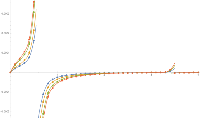
Figure 3: The ratio $A_{\Phi_{h_{1/4,-4},h_{1/4,4}}}/A_{\Phi_{h_{1/2,-2},h_{1/2,2}}}$ as a function of $Q$ for $L=5,6,7,8$ (blue, orange, green and red dots respectively). This ratio is generically non zero. It exhibits (in finite size) simple poles at $Q=4\cos^{2}{\pi\over 8}$, $Q=4\cos^{2}{4\pi\over 8}$, and vanishes exactly (in finite size) for $Q=0,3,4$.

While the amplitude is small in general, it is found to become large—nay divergent—for two special values:

$$Q = 4\cos^{2}{\pi\over 8}=3.414213\cdots\,,$$ (73a)

$$Q = 4\cos^{2}{3\pi\over 8}=0.585786\cdots\,.$$ (73b)

There are several ways to understand this. We will discuss a CFT analysis in the conclusion. From the lattice point of view, the divergence arises because the transfer matrix exhibits a Jordan cell in the lowest level of $\mathcal{W}_{4,\pm i}$. This Jordan cell arises from representation theory of the Jones algebra for $\mathfrak{q}=e^{i\pi/8},\mathfrak{q}=e^{3i\pi/8}$. To illustrate this, take for instance the case $\mathfrak{q}=e^{3i\pi/8}$. The module $\mathcal{W}_{2,-1}$ becomes reducible for this value of $\mathfrak{q}$, and admits a sequence of submodules as represented in Figure 4. The presence of submodules $\mathcal{W}_{4,i},\mathcal{W}_{4,-i}$ (in particular) suggests that excited states in $\mathcal{W}_{2,-1}$ (a module with two propagating clusters) mix with states in $\mathcal{W}_{4,i},\mathcal{W}_{4,-i}$ within the module involving four propagating clusters. This mixture leads to Jordan cells in the transfer matrix. As shown in (54)—and further discussed in Appendix B.4 in the case $Q=0$—a Jordan cell in turns translates into a contribution to the correlation function that is linear in (imaginary) time on the cylinder. This, finally, corresponds formally to an infinite amplitude.

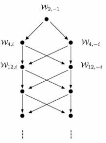
Figure 4: Sub-module structure of $\mathcal{W}_{2,-1}$ for $\mathfrak{q}=e^{3i\pi/8}$. Note the appearance of sub-modules isomorphic to $\mathcal{W}_{4,\pm i}$, which lead to glueing of standard modules into bigger, indecomposable modules, and Jordan cells for the transfer matrix.

5.3 The $s$-channel spectrum of $P_{aaaa}$: $F_{j,\mathrm{e}^{2i\pi p/M}}{\scriptstyle(M|j,~{}j\geq 2)}$, $j,jp/M$ even and $F_{0,-1}$

We now turn to $P_{aaaa}$: this is the probability that all four points belong to the same cluster. It is called $P_{0}$ in [1]. For all finite sizes, we find that the modules $\mathcal{W}_{j,e^{2i\pi p/M}}$ with $M|j,~{}j\geq 2$ and $j$ even contribute when $jp/M$ is even: this corresponds to the sectors with an even number of clusters propagating, and values of $z$ obeying $z^{j}=1$, what we have called earlier the $j$ even, S sectors. Geometrically, these contributions arise from configurations where for instance the points $1,3$ and $2,4$ are joined by two clusters which are only connected outside of the interval between their two (imaginary) time slices. On top of this, we also have the contribution where the four points belong to a single cluster arising between their two (imaginary) time slices. As discussed earlier, having a cluster propagating along the cylinder does not imply that there are boundaries around the cluster. The corresponding module of the Jones algebra is thus not a module with $j=1$: rather, it occurs as $\mathcal{W}_{0,-1}$, i.e., as a module with no through-lines, but for which non-contractible loops (which would cut the connection between $1,2$ and $3,4$) are forbidden.

Like for $P_{abab}$ and $P_{abba}$ we find that all eigenvalues in these modules do contribute in finite size, and that none of the amplitudes seem to vanish as $L\to\infty$. This suggests that the spectrum of critical exponents is given by $F_{j,\mathrm{e}^{2i\pi p/M}}{\scriptstyle(M|j,~{}j\geq 2)}$, $j,jp/M$ even and $F_{0,-1}$.

In the two clusters ($j=2$) sector, this leads to

$$(h_{e,-2};h_{e,2}),~{}~{}e\in\mathbb{Z}$$ (74)

while in the four clusters ($j=4$) sector we find

$$(h_{e,-4};h_{e,4}),~{}~{}e\in\mathbb{Z}$$

$$(h_{e+1/2,-4};h_{e+1/2,4}),~{}~{}e\in\mathbb{Z}$$ (75)

These two contributions occur as well in $S_{\mathbb{Z}+1/2,2\mathbb{Z}}$. New contributions appear for higher even values of $j$. For instance we find also

$$(h_{e,6};h_{e,-6}),~{}~{}e\in\mathbb{Z}$$

$$(h_{e\pm 1/3,6};h_{e\pm 1/3,-6}),~{}~{}e\in\mathbb{Z}$$ (76)

On top of this we have the ‘one-cluster sector’, which is described by $F_{0,-1}$ (i.e., non-contractible loops are killed). This corresponds to the set of conformal weights

$$(h_{e+1/2,0};h_{e+1/2,0}),~{}~{}e\in\mathbb{Z}$$ (77)

which is also in $S_{\mathbb{Z}+1/2,2\mathbb{Z}}$.

5.4 The $s$-channel spectrum of $P_{aabb}$: $F_{j,\mathrm{e}^{2i\pi p/M}}{\scriptstyle(M|j,~{}j\geq 2)}$, $j,jp/M$ even, $F_{0,-1}$ and $\bar{F}_{0,\mathfrak{q}^{2}}$

The quantity $P_{aabb}$ is the probability for two “short clusters” (as opposed to the “long clusters” shown in Figure 2): points $1,2$ belonging to one cluster, points $3,4$ to the other. It is called $P_{1}$ in [1]. We find that all the eigenvalues occurring in $P_{aaaa}$ also contribute to $P_{aabb}$. On top of these, we also find the eigenvalues from the module $\overline{\mathcal{W}}_{0,\mathfrak{q}^{2}}=\overline{\mathcal{W}}_{0,\mathfrak{q}^{-2}}$. This module corresponds to a sector with no (forced) propagating cluster, which is obtained simply by giving non-contractible loops their bulk weight. As usual now, none of the corresponding amplitudes seem to vanish in the limit $L\to\infty$.

The operator content from $\overline{\mathcal{W}}_{0,\mathfrak{q}^{\pm 2}}$ involves diagonal primaries, with weights

$$(h_{e+e_{0},0};h_{e+e_{0},0}),~{}~{}e\in\mathbb{Z}\,,$$ (78)

where

$$h_{e+e_{0},0}={[(m+1)(e+1)-1]^{2}-1\over 4m(m+1)}\,.$$ (79)

Of course this is the same set as the set

$$(h_{e,1};h_{e,1}),~{}~{}e\in\mathbb{Z}\,,$$ (80)

after a shift of the electric charge. We will denote this set as $\mathcal{S}^{d}_{\mathbb{Z},1}$.

5.5 Summary

We can now summarise our spectra in the $s$-channel

$$\begin{array}[]{c|ll}&\mbox{$s$-channel}&\mbox{Parities}\\ \hline\cr P_{aaaa}&\mathcal{S}_{1}\equiv\mathcal{S}_{\mathbb{Z}+1/2,0}\cup\{\mathcal{S}_{\mathbb{Z}+{p\over M},j}\}&j\in 2\mathbb{Z},\ jp/M\hbox{ even}\\ P_{aabb}&\mathcal{S}_{2}\equiv\mathcal{S}^{d}_{\mathbb{Z},1}\cup\mathcal{S}_{\mathbb{Z}+1/2,0}\cup\{\mathcal{S}_{\mathbb{Z}+{p\over M},j}\}&j\in 2\mathbb{Z},\ jp/M\hbox{ even}\\ P_{abab/abba}&\mathcal{S}_{3}\equiv\{\mathcal{S}_{\mathbb{Z}+{p\over M},j}\}&j\in 2\mathbb{Z},\ jp/M\hbox{ integer}\\ \hline\cr\end{array}$$ (85)

where we have allowed $j$ to take positive or negative values, since the sets of exponents are invariant under $j\to-j$. Recall that e.g. the set $\mathcal{S}_{\mathbb{Z},2\mathbb{Z}}$ refers to pairs of exponents $(h_{r,s},h_{r,-s})$ with $r\in\mathbb{Z},s\in 2\mathbb{Z}$, while $\mathcal{S}^{d}_{\mathbb{Z},1}$ denotes pairs $(h_{r,1},h_{r,1})$, with $r\in\mathbb{Z}$. Recall also that $p,M$ are coprime integers, and that the value $p=0$ in particular is allowed. The case ${p\over M}={1\over 2}$ appears already in [1].

Note that these are the generic results, i.e., those valid for $m$ irrational. Some contributions vanish for special values of $Q$, such as $Q=0$, $Q=2$ and $Q=4$ (see Appendix B) and in some cases Jordan blocks appear.

The spectra in the other channels follow from simple geometrical considerations:

$$\begin{array}[]{c|llc}&\mbox{$t$-channel}&\mbox{$u$-channel}\\ \hline\cr P_{aaaa}&\mathcal{S}_{1}&\mathcal{S}_{1}\\ P_{aabb}&\mathcal{S}_{3}&\mathcal{S}_{3}\\ P_{abab}&\mathcal{S}_{3}&\mathcal{S}_{2}&\\ P_{abba}&\mathcal{S}_{2}&\mathcal{S}_{3}&\\ \hline\cr\end{array}$$ (91)

An important property of our spectra in the case of $P_{aabb}$ is that only states with positive conformal weights propagate along the cylinder: no “effective central charge” appears, despite the non-unitarity of the CFT. This is contrast with what would be observed, for instance, in the case of minimal models corresponding to $m+1\equiv{p\over p^{\prime}}$, $p,p^{\prime}$ integer, where the effective ground state with $c_{\rm eff}=1-{6\over pp^{\prime}}$ would appear. It is our understanding that a similar phenomenon takes place in the conjectured expressions of [1].

6 Comparison with results in [1]

The comparison with the proposal in [1] requires some discussion, since the authors in this reference did not, in particular, provide conjectured results for $P_{aaaa}$. The simplest quantity to consider is $P_{abab}-P_{abba}\equiv P_{2}-P_{3}$ in the notations of that reference. Indeed, from eq. (3.2) in [1]

$$R_{\sigma}=\lambda(P_{0}+\mu P_{\sigma})$$ (92)

we see that, in their notations, $R_{2}-R_{3}=\lambda\mu(P_{2}-P_{3})$. The spectrum in the $s$-channel of $P_{2}-P_{3}=P_{abab}-P_{abba}$, according to our analysis, is made of the fields $(h_{e+p/M,-j};h_{e+p/M,j})$ for $e\in\mathbb{Z}$, with $j$ even and $pj/M$ an odd integer. Note that all these fields have $h-\bar{h}$ odd. In [1], meanwhile, the spectrum is $S_{\mathbb{Z}+1/2,2\mathbb{Z}}$ (after switching indices in[1] to make their conventions the same as ours), restricted like for us to odd spin $h-\bar{h}$. So for instance the field with weights $(h_{1/4,\mp 4};h_{1/4,\pm 4})$ for which we have seen that the amplitude is generically non-zero, is absent in the solution proposed in [1]. This suggests that their solution is, generically, not the correct one, and that an infinity of fields is missing in their proposal. We illustrate this qualitatively in Figures 5,6.

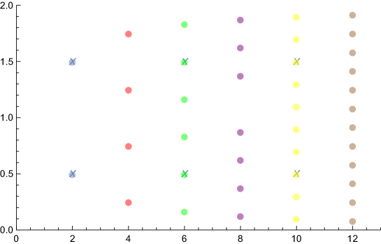
Figure 5: A sample of the full spectrum in the s-channel for $P_{abab}-P_{abba}$ represented by the pairs $(r,s)$ of the $h_{r,s}$ exponents ($r$ is on the y-axis, and $s$ on the x-axis. The spectrum considered in [1], depicted as crosses, is seen to be a tiny subset of the full spectrum: the projections of the dots on the y-axis in fact should cover it densely (represented here are exponents for $M=2,4,6,8,10,12$ only).

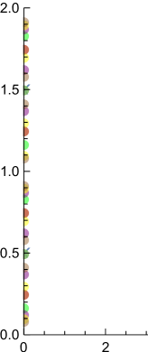
Figure 6: The projection on the vertical axis of the exponents represented in Figure 5

Meanwhile, it is fascinating to compare results for amplitudes that are predicted in [1] and which are also found to occur in our analysis. A good example of this is the first amplitudes for the sector with $j=2$, namely $A_{\Phi_{h_{3/2,-2},h_{3/2,2}}}$ and $A_{\Phi_{h_{1/2,-2},h_{1/2,2}}}$. The bootstrap in [1] produces amplitudes which are in fact simply related with those of Liouville field theory at $c<1$, and thus admit analytical expressions [49, 50]. In particular, their conjecture is

$${A_{\Phi_{h_{3/2,-2},h_{3/2,2}}}\over A_{\Phi_{h_{1/2,-2},h_{1/2,2}}}}=2^{-\frac{4}{\beta^{2}}}\frac{\Gamma(\frac{3}{2}+\frac{1}{4\beta^{2}})}{\Gamma(\frac{1}{4\beta^{2}})}\frac{\Gamma(\frac{3}{2}+\frac{3}{4\beta^{2}})}{\Gamma(1+\frac{3}{4\beta^{2}})}\frac{\Gamma(-1-\frac{1}{4\beta^{2}})}{\Gamma(\frac{3}{2}-\frac{1}{4\beta^{2}})}\frac{\Gamma(2-\frac{3}{4\beta^{2}})}{\Gamma(\frac{3}{2}-\frac{3}{4\beta^{2}})}$$ (93)

where $\beta^{2}={m\over m+1}$, $\sqrt{Q}=2\cos{\pi\over m+1}$, $m\in[1,\infty]$. This conjecture reproduces results which are believed to be exact at $Q=0,3,4$—the result for $Q=0$ is discussed in our Appendix B.4; the result for $Q=4$ follows from a work by A. Zamolodchikov (as discussed in [1]), and the result for $Q=3$ is unpublished work of R. Santachiara.

Numerical results for this ratio are given in figure 7. They are intriguingly close —after reasonable extrapolation—to the formula (93). The agreement is worse near $Q=4$, but as commented elsewhere in this paper, this discrepancy can possibly be attributed to the presence of a marginal operator affecting corrections to scaling. We do not know whether (93) might actually be exact, or whether it is just very close to the exact result. Numerics, at this stage, do not really allow us to settle this issue.

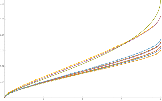
Figure 7: Results for the ratio $A_{\Phi_{h_{3/2,-2},h_{3/2,2}}}/A_{\Phi_{h_{1/2,-2},h_{1/2,2}}}$, as a function of $Q$, for sizes $L=5,6,7,8,9,10,11$ corresponding to colours blue, orange, green, red, purple, mauve, clear blue. The points in purple are obtained by extrapolating data for $L=5,7,9,11$ and those in yellow by extrapolating data for $L=6,8,10$. The green curve is the conjecture (93).

Meanwhile, the uncertainty of the numerical determination shown in Figure 7 can be estimated from the difference between the extrapolations through even and odd system sizes $L$. Given that this uncertainty is (for most values of $Q$) comparable to the distance to the conjectured result (93) is certainly a strong motivation for further improving the numerical algorithm and gain access to a few more sizes. This could maybe be achieved if one could impose the sector and momentum constraints within our scalar product method (see Appendix A.2).

7 Conclusion

We believe that the numerical and algebraic evidence presented in this paper invalidates the results in [1]. This is a very intriguing conclusion, since, in particular, the authors of [1] presented Monte Carlo simulations of four-point functions in the plane that were in good agreement with their bootstrap prediction. It is possible that the conjecture in [1], while not the correct answer to the problem of describing geometrical correlations in the Potts model, is indeed a solution to the bootstrap, and moreover captures numerically the essential features of the four-point functions, failing only at an accuracy, or for values of the cross-ratio $z$, not accessible using the Monte-Carlo approach. If this is the case, this raises several questions, in particular about the number of possible solutions to the bootstrap, and what, if anything, is truly described by the proposal in [1].

To shed more light on this issue, an obvious route is to build four-point functions following the methodology in [1] but based on our spectra. This is quite challenging technically, because of the large number of primary fields with dimensions of the same order of magnitude we would have to involve. Another, more fundamental aspect worth mentioning is that, in our spectrum, many of the conformal weights have degenerate values, with singular conformal blocks. It is not clear whether the regularisation procedure used in the bootstrap approach [1] is actually the relevant one for the $Q$-state Potts model. This, we believe, could be answered by numerical studies in the spirit of the present paper and [53].

A particularly intriguing fact is that we found numerically a ratio $A_{\Phi_{h_{3/2,-2},h_{3/2,2}}}/A_{\Phi_{h_{1/2,-2},h_{1/2,2}}}$ which is not incompatible with the proposal in [1]; see Figure 7. It could be that the solution to the bootstrap relevant for the Potts model involves for this ratio a value close to the one in [1] and yet different, over the whole range $Q\in[0,4]$. It could also be that the amplitudes in [1]—which, to the best of our understanding, are actually given by standard formulae for Liouville at $c<1$, naively extended to the case of fields with $h\neq\bar{h}$—are exact, but that something has to be added.

Adding “something” to the spectrum in [1] is definitely necessary if one wishes to avoid correlation functions with many singularities as $Q$ is varied. To see why this is the case, we consider the contributions to the antisymmetric combination of probabilities: including now higher order terms in the conformal blocks

$$P_{aabb}-P_{abba} \propto (z\bar{z})^{-2h_{1/2,0}}\left(A_{\Phi_{h_{1/2,-2},h_{1/2,2}}}{\cal F}_{h_{1/2,-2}}^{(s)}\overline{{\cal F}}_{h_{1/2,2}}^{(s)}\right.+$$ (94)

$$\left.A_{\Phi_{h_{3/2,-2},h_{3/2,2}}}{\cal F}_{h_{3/2,-2}}^{(s)}\overline{{\cal F}}_{h_{3/2,2}}^{(s)}+A_{\Phi_{h_{1/4,-4},h_{1/4.4}}}z^{h_{1/4,-4}}\bar{z}^{h_{1/4,4}}+\ldots\right)\,.$$

Note that we used here conformal blocks where the dependency $z^{-2h_{1/2,0}}$ (resp. $\bar{z}^{-2h_{1/2,0}}$) has been factored out.

When $Q\to 4\cos^{2}{3\pi\over 8}\equiv Q^{*}$, we find that $h_{3/2,2}\to h_{1,2}$, a degenerate value. The conformal block in the four-point function coming from

$$(h_{3/2,-2},h_{3/2,2})=(h_{3/2,-2},h_{1,2})=\left(-{1\over 32}+3,-{1\over 32}\right)$$ (95)

has a null-state at level 2 for the $\bar{z}$ components, with weights

$$(h_{3/2,-2},h_{1,-2})=\left(-{1\over 32}+3,-{1\over 32}+2\right)\,.$$ (96)

The appearance of the null-state means that the conformal block $\overline{{\cal F}}_{h_{3/2,2}}$ has a pole of the form ${1\over Q-Q^{*}}$ multiplying the term $z^{h_{3/2,-2}}\bar{z}^{h_{1,-2}}$. Setting

$${\cal F}_{h_{3/2,-2}}^{(s)}\overline{{\cal F}}_{h_{3/2,2}}^{(s)}\approx\ldots+{r^{*}\over Q-Q^{*}}z^{h_{3/2,-2}}\bar{z}^{h_{3/2,2}+2}+\ldots\,,$$ (97)

we see that the amplitude of the singular term in the bracket in (94) is

$$A_{\Phi_{h_{3/2,-2},h_{3/2,2}}}{r^{*}\over Q-Q^{*}}z^{h_{3/2,-2}}\bar{z}^{h_{3/2,2}+2}\,.$$ (98)

Meanwhile we observe that the weights for the singular term coincide with the weights from the $1/4$ sector:

$$(h_{1/4,-4},h_{1/4,4})=\left({-1\over 32}+3,{-1\over 32}+2\right)\,.$$ (99)

Recall that we have found numerically that the amplitude of this field also has a simple pole when $Q\to Q^{*}$:

$$A_{\Phi_{h_{1/4,-4},h_{1/4,4}}}\approx{R\over Q-Q^{*}}\,,$$ (100)

so the amplitude of the second singular term in (94) is

$${R\over Q-Q^{*}}z^{h_{1/4,-4}}\bar{z}^{h_{4,1/4}}\,.$$ (101)

For technical reasons, we normalise all quantities by $A_{\Phi_{h_{1/2,-2},h_{1/2,2}}}$ (this amplitude is not expected to be singular), so we set

$${A_{\Phi_{h_{1/4,-4},h_{1/4,4}}}\over A_{\Phi_{h_{1/2,-2},h_{1/2,2}}}}\approx{r\over Q-Q^{*}}\,.$$ (102)

We find numerically that on “resonance”, there is a Jordan cell of rank two mixing the two terms, but no singularity. This means that we should have the condition

$$r+{A_{\Phi_{h_{3/2,-2},h_{3/2,2}}}\over A_{\Phi_{h_{1/2,-2},h_{1/2,2}}}}r^{*}=0\,.$$ (103)

To put things differently, the appearance of a null-state in the conformal block $\overline{{\cal F}}_{h_{3/2,2}}$ leads to a divergence in the four-point function (assuming the formula for $A_{\Phi_{h_{3/2,-2},h_{3/2,2}}}$ given earlier is correct). To cancel this divergence, a contribution $A_{\Phi_{h_{1/4,-4},h_{1/4,4}}}$ is necessary. Moreover, this contribution must exhibit a simple pole, as we have observed numerically. It is possible that this picture generalises, with singularities in the proposal of [1] exactly cancelled out by the additional terms we find in our lattice analysis. This will be discussed elsewhere [54].

To conclude this paper, we re-iterate the remark that the eigenvalues contributing to the probabilities are (a subset of) those appearing in the Potts model partition function [7]. While this would be a well expected fact for a model defined locally such as the Ising model or any kind of height model, this is not so obvious in our case. Indeed, in a model where correlations are defined non-locally there is no clear connection between the partition function and at least some of the observables. To give a simple example, we know well that the probability that two points are connected with a cluster allowing two independent paths involves exponents not present in the partition function [33, 35]. The fact that no such exponents are needed for the $P_{a_{1}a_{2}a_{3}a_{4}}$ suggests that these are rather close to “ordinary” observables, and that we may be able to understand them in terms of fully local operators acting on the space of states. One of the main “elementary” mysteries in this description is why only sectors with an even number of clusters contribute. We believe that thinking more deeply about algebraic aspects of the problem on the lattice will shed some light on this question.

Acknowledgements.

We thank the authors of [1] and especially S. Ribault for inspiring discussions. We also thank C.R. Scullard for discussions about numerical aspects and especially for the use of his unpublished C++ implementation of the Arpack version of the Arnoldi algorithm. This work was supported by the ERC Advanced Grant NuQFT.

Appendix A Computing four-point functions on the cylinder

In this appendix we gather all the algebraic and numerical technology that enables us to compute four-point functions in the FK cluster model on a cylinder.

The geometrical setup is shown in Figure 1. For the sake of simplicity we shall define the model on an axially oriented square lattice of width $L$ spins. The four points are inserted in two different time slices, separated by $l$ lattice spacings, with points $w_{1},w_{2}$ in the first slice and points $w_{3},w_{4}$ in the second slice.

The algebraic tool is the transfer matrix $T$ based on the join-detach algebra, which we have already briefly reviewed in section 3.1. To adapt it to the computation of correlation functions the crucial point is the representation of the algebra, i.e., the choice of the set of states on which $T$ acts. While the partition function $Z$ can be simply computed by taking these states to be set partitions of $L$ points (see [55, 56] for details) we shall need to endow these partitions with various kinds of marks.

We are interested in two different situations that present some subtle differences. First we describe how to compute directly the 15 different FK cluster correlation functions $P_{a_{1},a_{2},a_{3},a_{4}}$, defined by (6), that lie at the heart of the numerical method outlined in section 4.3.1. Second, we go into the details of the alternative method of section 4.3.2 which is based on computing scalar products involving the order parameter operators (5).

A.1 Computation of $P_{a_{1},a_{2},a_{3},a_{4}}$

Let $w_{k}$ (with $k=1,2,3,4$) be four marked points on the cylinder, as shown in Figure 1. Let ${\cal P}=\{a_{1},a_{2},a_{3},a_{4}\}$ be a set partition of the four points, defined by the corresponding integer labels $a_{k}$. We wish to construct a transfer matrix that builds the statistical weight $W_{\cal P}$ corresponding to a correlation function in which the marked points $k$ and $\ell$ belong to identical (resp. different) FK clusters if $a_{k}=a_{\ell}$ (resp. $a_{k}\neq a_{\ell}$). For instance, the choice ${\cal P}=\{1,2,1,2\}$ means that $w_{1}$ and $w_{3}$ belong to the same cluster, while $w_{2}$ and $w_{4}$ also belong to a common cluster which is different from the first one, as shown in the left panel of Figure 2.

On the cylinder there are $B_{4}=15$ different correlation functions, where the Bell number $B_{N}$ denotes the number of partitions of an $N$-element set. On the strip there would be only $C_{4}=14$ correlation functions, where $C_{N}$ denote the Catalan numbers.

We consider the square lattice of width $L$ wrapped on a cylinder. The sites within each row are labelled by $i=0,1,\ldots,L-1$, with the labels considered modulo $L$ by the periodic boundary conditions. To make contact with Figure 1, we let $w_{1}$ and $w_{2}$ correspond to sites $0$ and $2a$ (with $a\in\mathbb{N}/2$) in the row labelled by the transfer matrix “time” $t_{1}=0$, while $w_{3}$ and $w_{4}$ correspond to sites $x$ and $x+2a$ in the row $t_{2}=l$. A cluster containing (at least) one of the points $w_{k}$ is called a marked cluster.

To allow the marked clusters to wind around their insertion points, we consider a larger piece of the lattice, going from row $t_{0}=-M$ to row $t_{3}=l+M$. We impose free boundary conditions on the two extremites of the finite cylinder defined by $t\in[t_{0},t_{3}]$. The desired correlation functions (or probabilities) are then given by the limit

$$P_{\cal P}(l)=\lim_{M\to\infty}\frac{W_{\cal P}}{\sum_{r=1}^{15}W_{{\cal P}_{r}}}\,.$$ (104)

For practical purposes, to obtain $P_{\cal P}(l)$ to a given numerical precision, it suffices to take $M$ sufficiently large, so that the results for $M$ and $M+1$ coincide to the chosen precision. A more precise criterion for the choice of $M$ can be given once the spectrum of the transfer matrix is known (see section A.7.2).

The transfer matrix acts as usual on states $\{s_{1},s_{2},\ldots,s_{L}\}$ which are certain set partitions of $L$ points, but now endowed with suitable markings. We have $s_{i}=s_{j}$ if and only if sites $i$ and $j$ are seen to be in the same FK cluster at a given time $t$—by this we mean that $i$ and $j$ are connected by a piece of FK cluster on the partly constructed cylinder $t\in[t_{0},t]$. The symbols $s_{i}$ can take the values $1,2,\ldots,L$ for unmarked clusters, and $\bar{1},\bar{2},\bar{3},\bar{4}$ for marked clusters containing one of the points $w_{k}$. If a marked cluster contains more than one marked point, the chosen symbol is the lowest one, in order to avoid any redundancy in the correspondence between cluster connectivities and states. Unmarked clusters are indistinguishable.

As shown in (11) the transfer matrix can be written as a product of elementary operators ${\sf H}_{i}={\sf I}+v{\sf J}_{i}$ and ${\sf V_{i}}=v{\sf I}+{\sf D}_{i}$ that add respectively a horizontal edge between sites $i$ and $i+1$ (mod $L$), and a vertical edge on top of site $i$. We have $v={\rm e}^{K}-1$, with $K$ the Potts coupling, and the critical value on the square lattice is $v_{\rm c}=\sqrt{Q}$. The join and detach operators, ${\sf J}_{i}$ and ${\sf D}_{i}$ satisfy the join-detach algebra with relations (12). We now describe a modified representation of this algebra that properly takes into account the possibility of having marked clusters.

A clusters is said to be left behind at site $i$ if ${\sf D}_{i}$ detaches a singleton in the set partition. When this happens, ${\sf D}_{i}$ applies a weight $Q$, irrespective of whether the cluster being left behind is unmarked or marked.

Remark 8.

In some applications it is natural to give weight $1$ to marked clusters. In particular, this is mandatory in the limit $Q\to 0$, since otherwise all correlation functions would be identically zero. However, for the time being we choose to give weight $Q$ to any cluster, including the marked ones, since then $\sum_{r=1}^{15}W_{{\cal P}_{r}}=Z(Q,v)$, the partition function on a cylinder of circumference $L$ and length $l+2M$. The quantity $Z(Q,v)$ can easily be obtained by independent means [57], and the sum rule then provides a valuable check of the correctness of the algorithm.

To apply the initial condition, we start from the all-singleton state $\{1,2,\ldots,L\}$ at time $t_{0}$. The final condition at time $t_{3}$ is to project out any state in which the desired connections between marked clusters have not been achieved. To be precise, if there exists two distinct labels $\bar{k}\neq\bar{\ell}$ in the connectivity state such that $a_{k}=a_{\ell}$, then the state must be discarded. Any state that survives this projection is attributed a weight $Q$ per cluster (again irrespectively of whether it is unmarked or marked). The weighted sum over retained states produces the sought-for $W_{\cal P}$.

Marked symbols are introduced in the time evolution by joining site $i=0$ (resp. $i=2a$) to the marked symbol $\bar{1}$ (resp. $\bar{2}$) at time $t=t_{1}$, and by joining site $i=x$ (resp. $i=x+2a$) to the marked symbol $\bar{3}$ (resp. $\bar{4}$) at time $t=t_{2}$.

To impose the desired four-point connectivity, we modify the action of the join operators ${\sf J}_{i}$ as follows:

• When ${\sf J}_{i}$ joins an unmarked cluster to a marked cluster with symbol $\bar{k}$, the result is a marked cluster with the same label $\bar{k}$.

• ${\sf J}_{i}$ can join two marked clusters with labels $\bar{k}$ and $\bar{\ell}$ only if $a_{k}=a_{\ell}$. In that case, the result is a marked cluster with the lowest label ${\rm min}(\bar{k},\bar{\ell})$.

The detach operators ${\sf D}_{i}$ need a more subtle modification. We describe the marked points $w_{1}$ and $w_{2}$ as unseen (i.e., not yet visited by the transfer process) when the time $t<t_{1}$. Similarly the marked points $w_{3}$ and $w_{4}$ are unseen when $t<t_{2}$. The required modification is:

• The cluster $\bar{k}$ is allowed to be left behind only if the label $a_{k}$ is different from the labels of any other marked cluster in the connectivity state, and also different from the labels of all yet unseen marked points.

A.1.1 Example

Consider the case ${\cal P}=\{a_{k}\}=\{1,2,1,2\}$ of two propagating clusters. At times $t_{1}<t<t_{2}$, the points $w_{1}$ and $w_{2}$ have been seen, so the connectivity state can contain the symbols $\bar{1}$ and $\bar{2}$. In fact, both symbols must be present, because the ${\sf J}_{i}$ operator cannot join $\bar{1}$ and $\bar{2}$ (since we have $a_{1}\neq a_{2}$); moreover none of them can be left behind, because points $P_{3}$ and $P_{4}$ are unseen. Indeed, $a_{1}=a_{3}$ then prevents $\bar{1}$ from being left behind, and $a_{2}=a_{4}$ prevents $\bar{2}$ from being left behind.

At later times $t_{2}<t<t_{3}$, all points have been seen. Symbols $\bar{1}$ and $\bar{3}$ can join, because $a_{1}=a_{3}$ (and similarly for $\bar{2}$ and $\bar{4}$). But before this happens, none of the clusters $\bar{1}$ and $\bar{3}$ can be left behind (by the rule on ${\sf D}_{i}$). When $\bar{1}$ and $\bar{3}$ join, the resulting cluster carries the symbol $\bar{1}$ (by the second rule on ${\sf J}_{i}$). After this happens, $\bar{1}$ can be left behind (by the rule on ${\sf D}_{i}$, because $\bar{3}$ is no longer used in the connectivity state).

A.1.2 Checks

In addition to extensive checks for small systems, where all configurations can be drawn by hand, we have checked that:

1. The unnormalised sum $\sum_{r=1}^{15}W_{{\cal P}_{r}}=Z(Q,v_{\rm c})$ for any values of $Q$, $L$, $l$, and $M$.

2. The probabilities converge to any desired numerical precision upon taking $M\gg L,l$ large enough.

Moreover, for the situation with shift $x=0$ (see Figure 1) it is non-trivial from the point of view of the transfer algorithm that the following lattice symmetries hold true:

1. The four probabilities in which three points are in the same cluster are all equal.

2. The six probabilities in which two points are in the same cluster and the other two are in two distinct clusters, are equal two by two.

A more restricted set of lattice symmetries holds true also for $x\neq 0$; for instance the four probabilities in which three points are in the same cluster, are equal two by two. We have checked this as well.

A.1.3 Sample results

To help the readers desirous of writing their own implementation, we here give some sample results for $\mathbb{P}_{\cal P}(l)$ for a system with $Q=1$ and size $L=5$. We take distance $l=3$ between the time slices and place the points in each slice as nearest neighbours ($2a=1$), with no offset between the two slices ($x=0$). The set of 15 probabilities (up to the symmetries described above) are then:

$$P_{aaaa} = 0.4137474261084028402728075794444609019425125830604\,,$$ (105a)

$$P_{aaab} = 0.0527654414874488570020983215187468064670272213592\,,$$ (105b)

$$P_{aabb} = 0.1710044985220526406478058107746167574154887333139\,,$$ (105c)

$$P_{abab} = 0.0008428892255516309347686777944043427144862186950\,,$$ (105d)

$$P_{abba} = 0.0000809519640647414138510576682844254047786037826\,,$$ (105e)

$$P_{aabc} = 0.0728732174729894992103081083804105937132582003470\,,$$ (105f)

$$P_{abac} = 0.0082903229000495425925235985388971176349864439965\,,$$ (105g)

$$P_{abca} = 0.0061033620128809220144422552541186396032488302690\,,$$ (105h)

$$P_{abcd} = 0.0287286634582927910878256638963936447516380264857\,.$$ (105i)

It was necessary to take $M=200$ to achieve 50 correct digits. Note that our code is written so that the number of digits of numerical precision can be adjusted to any desired value.

As a final check we consider the limit $l\gg L$. Then we expect

$$P_{abcd} = (1-p)^{2}\,,$$ (106a)

$$P_{aabc} = p(1-p)\,,$$ (106b)

$$P_{aabb} = p^{2}\,,$$ (106c)

where $p$ is the finite probability that two nearest neighbours are in the same cluster. All other $P_{{\cal P}_{r}}(l)$ will be negligible in that limit. By taking $L=5$ and $l=384$ (with still $M=200$) we have verified that this is indeed the case, and we estimate

$$p=0.76315602507834269413\,.$$ (107)

A.1.4 Case of $Q\to 0$

The limit $Q\to 0$ (with $v=\sqrt{Q}\to 0$ as well) is somewhat special from the point of view of normalisations, since then $Z(Q,v)=0$. The partition function which is used to normalise the weights $W_{\cal P}$ and turn them into probabilities, as in (104), is then taken as $\widetilde{Z}=W_{aaaa}$, the number of spanning trees containing all four marked points. Moreover, any marked cluster is assigned a weight $1$ (instead of $Q$ in the general case), whereas unmarked clusters still have the weight $Q=0$, which implies that such clusters are disallowed.

A.2 Computation of $G_{a_{1},a_{2},a_{3},a_{4}}$

The second numerical method presented in section 4.3.2 provides a means of computing one by one the amplitudes appearing in the order parameter correlation functions $G_{a_{1},a_{2},a_{3},a_{4}}$ defined in (7). This method is of a very different nature than the one just presented (i.e., for the computation of $P_{a_{1},a_{2},a_{3},a_{4}}$), since it does not compute the four-point correlator directly on a cylinder of finite length, but rather goes directly for the asymptotic quantities $A_{i}$. Thus, the appearance of $|v_{0}\rangle$ and $\langle v_{0}|$ in (57) amounts effectively to taking the limit $M\to\infty$ of the distance to the boundary conditions, and the piece $|v_{i,j}\rangle\,\langle v_{i,j}|$ projects directly on an intermediate state in the $s$-channel, which is equivalent to taking the limit $l\to\infty$.

As a prerequisite to this approach—and in order recover in particular the same results as with the first method of section 4.3.1—it is however necessary to produce yet another representation of the join-detach algebra. In particular, we shall need the action of the order parameter operators ${\cal O}_{a}$ to be well-defined for generic values of $Q\in\mathbb{R}$. By (5), this hinges on giving a well-defined meaning—and in particular, a meaning that extends to non-integer $Q$—to the operator $\delta_{\sigma_{k},a}$ that fixes the value of the spin at point $w_{k}$ to be equal to the label $a$. Note that such extensions of order-parameter related quantities have played an important role in several recent pieces of work involving the present authors [11, 12, 13, 19, 20, 21].

As stated around (9) we are here only interested in correlation functions $G_{a_{1},a_{2},a_{3},a_{4}}$ employing at most two distinct symbols, $a$ and $b$. We shall therefore take $T$ to act on basis states which are set partitions of $L$ points with two marked values, denoted $a$ and $b$. It is crucial that these values are now different by definition. This provides a difference with the computation of $P_{a_{1},a_{2},a_{3},a_{4}}$, where two differently marked clusters could be joined under some circumstances. More precisely, the rules are now the following:

• The operator $\delta_{\sigma_{k},a}$ (the non-trivial part of ${\cal O}_{a}$) acts at the point $w_{k}$ by transforming an unmarked cluster touching that site into a marked cluster of label $a$. If the cluster is already marked with label $b$, ${\cal O}_{a}$ acts as the identity times $\delta_{a,b}$.

• The join operator ${\sf J}_{i}$ acts as usual on two unmarked clusters. When acting on an unmarked cluster and a marked cluster of label $a$, the result is a marked cluster of label $a$. Finally, when acting on two marked clusters of labels $a$ and $b$, ${\sf J}_{i}$ acts as the identity times $\delta_{a,b}$.

• The detach operator ${\sf D}_{i}$ transforms site $i$ into an unmarked singleton. If $i$ was already a singleton beforehand, a weight $Q$ is applied if the corresponding cluster is unmarked, and $1$ if it is marked.

To compute the scalar products in (57) it is convenient to produce all the intervening vectors in the same space. In particular, the ground state eigenvector $|v_{0}\rangle$ is written within the space of set partitions with two marked values, although it is easily seen that its component along any state containing marked clusters is zero.

A.2.1 Orthogonalisation

It has already been stated in the main text that the scalar product method relies on the left and right eigenvectors being orthogonal, even within degenerate subspaces. Standard numerical methods for non-symmetric matrices, such as the Arnoldi algorithm, do not immediately produce the eigenvectors in this form. Rather, within each degeneral subspace corresponding to the eigenvalue $\Lambda_{i}$, the scalar product of eigenvectors come out as

$$\langle v_{i,j}|v_{i^{\prime},j^{\prime}}\rangle=\alpha^{(i)}_{j,j^{\prime}}\,,$$ (108)

where the nombers $\alpha^{(i)}_{j,j^{\prime}}$ can be viewed as the elements of some matrix $\alpha^{(i)}$. However, if we replace the right eigenvectors by the linear combinations

$$|\widetilde{v}_{i^{\prime},j^{\prime}}\rangle=\sum_{k}\beta^{(i)}_{kj^{\prime}}|v_{i,k}\rangle$$ (109)

it is easy to see that we obtain the orthonormality $\langle v_{i,j}|\widetilde{v}_{i^{\prime},j^{\prime}}\rangle=\delta_{j,j^{\prime}}$ provided we take $\beta^{(i)}=\left(\alpha^{(i)}\right)^{-1}$. In practice, the size of degenerate subspaces is rather small (of dimension $1,2,4$ or $8$ in the problem at hand), and so any elementary method of producing the inverse matrix $\left(\alpha^{(i)}\right)^{-1}$ will solve the problem conveniently.

A.2.2 Checks

We have made extensive checks that the $A_{i}$ obtained from the scalar product method are identical to those obtained from the more involved first method based on (53), provided one takes into account the linear relations (9), and forms the sum over orthogonalised degenerated subspaces in (57).

We have verified that the scalar product method also gives the correct amplitudes of $G_{aaaa}$ in the simpler case where the states of $T$ are constrained to have only one marked value $a$. It seems likely—although we have not actually tried this—that it will also extend to the most general $G_{a_{1},a_{2},a_{3},a_{4}}$ provided the number of marked values is (at least) equal to the number of different symbols $a_{k}$ in the correlation fucntion.

A.3 Spectrum of $T$

At many occasions throughout this work we need to obtain the eigenvalues $\Lambda_{i}$ of the transfer matrix. This is obviously a much easier problem than obtaining the correlation functions, and has been discussed in many places, so we can be rather brief.

A.3.1 First representation

The $\Lambda_{i}$ are related to the asymptotic decay of the two-point functions, so in analogy with section A.1 they can be obtained by using the representation of the join-detach algebra in the regime $t_{1}<t<t_{2}$, where the boundary conditions $t_{1}\to-\infty$ and $t_{2}\to\infty$ have been pushed to the extremities of the cylinder. More precisely, we are interested in the sector with $\ell$ propagating FK clusters, so we can build on the same representation as in section A.1, but with states employing $\ell$ distinct marked symbols. The action of the elementary operators ${\sf J}_{i}$ and ${\sf D}_{i}$ must ensure that $\ell$ distinct clusters propagate along the cylinder, and the rules match those of section A.1 for $t_{1}<t<t_{2}$:

• ${\sf J}_{i}$ cannot join two marked clusters corresponding to different labels.

• ${\sf D}_{i}$ cannot leave behind any marked cluster.

• The different labels are treated as indistinguishable.

The last rule means that if the first site in the cluster with mark $\bar{k}$ is denoted $i_{k}$, we quotient the set of states in order to impose $i_{1}<i_{2}<\ldots<i_{\ell}$.

We have checked that the spectrum of this transfer matrix coincides with that of the loop model (3) in the affine TL representations (22), where as usual $j=\ell$ for $j\geq 2$, while the first and the third terms in the direct sum correspond to $\ell=0$ and $\ell=1$ respectively.

A.3.2 Second representation

It is also of interest to express $T$ in the representation of section A.2. There are now precisely two different marks, and the rules read:

• ${\sf J}_{i}$ cannot join two marked clusters corresponding to different labels.

• ${\sf D}_{i}$ can leave behind a marked cluster (with weight 1).

• The different labels are treated as distinguishable.

We find that the spectrum of this transfer matrix reproduces precisely (22), but only for $j=0,2,4,\ldots$, including the structure $\overline{\mathcal{W}}_{0,\mathfrak{q}^{\pm 2}}\oplus~{}\mathcal{W}_{0,-1}$ with two direct summands for $j=0$ and the absence of (at least the first few) odd terms ($j=1,3$). At present it is not obvious to us what is the precise decomposition of this representation in terms of simple affine TL modules, but we take the observations just mentioned as a first sign that our main result on the $s$-channel of four-point functions might have a natural interpretation within this representation of the join-detach algebra. We therefore suggest that it might be worthwhile to study more precisely the algebra obtained from generators ${\cal O}_{a}(\sigma_{i})$, ${\sf J}_{i}$ and ${\cal D}_{i}$, which contains the usual join-detach algebra as a sub-algebra.

A.4 Momentum sectors of $T$

As discussed in section 4.3.3, it is important to be able to associate the eigenvalues $\Lambda_{i}$ of $T$ with the conformal properties that emerge in the continuum limit. To this end we shall need to attach to each $\Lambda_{i}$ more information than just the number of propagating FK clusters that it corresponds to.

It is most practical for our purposes to consider here the loop model, in its representation of standard modules $\mathcal{W}_{j,z^{2}=\mathrm{e}^{2iK}}$ within the affine TL algebra $\mathsf{T}^{a}_{N}(n)$. We denote in this section by $T_{N,2\ell}$ the corresponding transfer matrix on link patterns with $N=2L$ strands (recall that $L$ is the number of Potts spins in a row) and $2\ell$ through-lines. Each through-line picks up a factor $z$ (resp. $z^{-1}$) when it traverses the periodic boundary condition towards the right (resp. left).

Our goal is to make apparant two more quantum numbers: the momentum $k$ of the through-lines, and the lattice momentum $m$. The former comes directly from the quantisation of $z$, and the latter is equal, in finite size, to the conformal spin: $m=h-\bar{h}$. We shall obtain each momentum sector by transforming $T_{N,2\ell}$ into an appropriate matrix of smaller dimension.

To this end we proceed as follows. The dimension of $W_{j,z}$ is ${N\choose N/2-j}$. Within this space we choose one representative state for each orbit of the cyclic group $C_{L}$ generated by $u^{2}$, where $u$ is the affine TL shift operator. Note that $[T_{N,2\ell},u^{2}]=0$ for the Potts-model transfer matrix. The orbit length corresponding to a representative state $|s\rangle$ is denoted $g_{s}$, so the orbit can be written

$$|s\rangle,u^{2}|s\rangle,u^{4}|s\rangle,\ldots,u^{2(g_{s}-1)}|s\rangle\,.$$ (110)

Obviously $g_{s}$ is a divisor of $L$, and the weighted sum over representative states (with each $|s\rangle$ being weighted by its orbit length $g_{s}$) equals $\mbox{dim}\,W_{j,z}$.

Example 1.

For $L=3$ and $\ell=0$ the dimension of $W_{j,z}$ is ${6\choose 3}=20$ (we do not need to take the quotient yet), and there are 8 distinct orbits (namely 6 with $g_{s}=3$, and 2 with $g_{s}=1$). For $L=8$ and $\ell=4$ the dimension of $W_{j,z}$ is ${16\choose 4}=1820$, and there are 224 orbits with $g_{s}=8$, 6 orbits with $g_{s}=4$, and 2 orbits with $g_{s}=2$.

The motion within orbits gives rise to another momentum variable, distinct from the twist $z$ of the affine TL algebra. Recall that the twist variable is $z={\rm e}^{i\pi k/\ell}$ for each through-line traversing the seam towards the right, and since the total phase factor for a turn of all $2\ell$ through-lines must be $z^{2\ell}=1$ we have $k=0,1,\ldots,\ell-1$. Similarly we now wish to construct the sector of lattice momentum $\omega_{m}\equiv(\omega)^{m}$, where $\omega\equiv{\rm e}^{2\pi i/L}$, by attributing a weight $\omega_{m}$ to each translation of one Potts spin (hence two TL loop strands) within the orbits of $C_{L}$. Since the total phase factor for a rotation through $L$ spins must be $(\omega_{m})^{L}=1$ we have $m=0,1,\ldots,L-1$. We stress that $k$ is related to the number of FK clusters $\ell$, whereas $m$ is related to the system size $L$.

We now wish to construct a restriction $T_{N,2\ell,m}$ to given values of the momentum labels $k\in\mathbb{Z}_{\ell}$ and $m\in\mathbb{Z}_{L}$. This means that the spectrum of $T_{N,2\ell}(n,z)$ must be decomposed as the union of the spectra of $T_{N,2\ell,m}$, including multiplicities:

$$\mbox{spec}\,T_{N,2\ell}(n,z)=\bigcup_{m=0}^{L-1}\mbox{spec}\,T_{N,2\ell,m}(n,z,\omega_{m})\,.$$ (111)

It is practical for us to denote the set of eigenvalues of $T_{N,2\ell,m}(n,z,\omega_{m})$, with specified values of the momenta $z={\rm e}^{i\pi k/\ell}$ and $\omega_{m}={\rm e}^{2i\pi m/L}$, simply as $V_{\ell,k,m}$. We denote the revelant dimensions as $D_{\ell}=\mbox{dim}\,W_{j,z}$ and $d_{\ell,k,m}=\mbox{dim}\,V_{\ell,k,m}$, where $d_{\ell,k,m}$ will be determined below. We should of course have

$$D_{\ell}=\sum_{m=0}^{L-1}d_{\ell,k,m}$$ (112)

for any $\ell=0,1,\ldots,L$ and $k\in\mathbb{Z}_{\ell}$, in accordance with (111).

Our approach is to construct, for each $m$, a $D_{\ell}\times d_{\ell,k,m}$ matrix $S_{\text{in}}$, and a $d_{\ell,k,m}\times D_{\ell}$ matrix $S_{\text{out}}(z,\omega)$, such that

$$T_{N,2\ell,m}(n,z,\omega_{m})=S_{\text{out}}(z,\omega)T_{N,2\ell}(n,z)S_{\text{in}}\,.$$ (113)

In the matrix $S_{\text{in}}$, each state $|s\rangle$ in the restricted space is mapped to the corresponding representative state in the full space, with a Boltzmann weight equal to $g_{s}$. In other words, if the representative state $|s\rangle$ is ordered as the $j$’th basis state in the restricted space and as the $i$’th basis state in the full space, then $(S_{\text{in}})_{ij}=g_{s}$. All other matrix elements are zero.

In the matrix $S_{\text{out}}(z,\omega)$, each state $|t\rangle$ in the full space is identified as $|t\rangle=u^{2k}|s\rangle$, where $|s\rangle$ is the representative state corresponding to $|t\rangle$ (i.e., with $|s\rangle$ living in the restricted space) and $k$ the number of double shifts (by convention, towards the left) necessary to bring $|t\rangle$ into the representative form. Notice that under these shifts, it is possible that a number of through-lines $p$ will cross the periodic boundary condition (towards the left). We must keep in mind that the convention for $\mathsf{T}^{a}_{N}(n)$ is that each through-line that crosses the periodic boundary condition towards the right (resp. left) acquires the weight $z$ (resp. $z^{-1}$). Therefore, the Boltzmann associated with bringing $|t\rangle$ into the representative form $|s\rangle$ is $(\omega_{m})^{k}z^{-p}/g_{s}$. Thus, if $|t\rangle$ is ordered as the $j$’th basis state in the full space and its representative $|s\rangle$ is the $i$’th basis state in the restricted space, then

$$(S_{\text{out}}(z,\omega))_{ij}=\frac{(\omega_{m})^{k}}{g_{s}z^{p}}=\frac{\omega^{m\cdot k}}{g_{s}z^{p}}\,.$$ (114)

All other matrix elements are zero.

A crucial point is that the orbit lengths must be compatible with the momentum that we impose. To be precise, the restricted states corresponding to given values of the labels $k,m$ are those with orbit lengths $g_{s}$ satisfying

$$(k-m)g_{s}=0\mbox{ mod }L\,.$$ (115)

The dimension $d_{\ell,k,m}$ is precisely determined by the number of restricted states satisfying this constraint.

Example 2.

Let us consider again the case $L=8$ and $\ell=4$. Any $V_{\ell,k,m}$ with $k-m\in 4\mathbb{Z}$ comprises all $224+6+2=232$ representative states (corresponding to $g_{s}=8,4,2$), so that the corresponding $d_{\ell,k,m}=232$. When $k-m\in 4\mathbb{Z}+2$ only the states with $g_{s}=8,4$ are allowed, so that $d_{\ell,k,m}=230$. And finally, when $k-m\in 2\mathbb{Z}+1$, only the states with $g_{s}=8$ are allowed, so that $d_{\ell,k,m}=224$. To obtain the sumrule (112) we notice that for any $k\in\mathbb{Z}_{\ell}$, the eight values of $m\in\mathbb{Z}_{L}$ corresponds to $8$ cases where $g_{s}=8$ is allowed, $4$ cases where $g_{s}=4$ is also allowed, and $2$ cases where $g_{s}=2$ is also allowed, i.e., we recognise the values of the $g_{s}$ themselves in this count. Thus $8\times 224+6\times 4+2\times 2=1820$, as it should. By the same reasoning, (112) is verified for arbitrary values of $L$ and $\ell$.

We have written an algorithm that produces the basis change matrices $S_{\text{in}}$ and $S_{\text{out}}(z,\omega)$ very efficiently. The crux is obviously to deal with the ordering of the states and the identification of the relevant orbits. We stress that the construction with basis change matrices $S_{\text{in}}$ and $S_{\text{out}}(z,\omega)$ is perfectly compatible with iterative diagonalisation schemes (such as the Arnoldi method), which are particularly efficient for dealing with transfer matrices that allow for a sparse matrix factorisation.

Finally we note that the spaces $V_{\ell,k,m}$ are invariant upon simultaneously changing the signs of both momenta (modulo $\ell$ and $L$, respectively). Thus

$$V_{\ell,k,m}=V_{\ell,\ell-k,L-m}\,.$$ (116)

We have checked this exhaustively for $L=5$ and $L=6$.

A.4.1 Checks

To check the algorithm, we have performed extensive tests on the case $N=2L=10$. We have first checked that $[u^{2},T_{N,2\ell}(n,z)]=0$ for $\ell=0,1,\ldots,L$ and any values of $n=\sqrt{Q}$ and $z$.

The sector decomposition was checked in details for a generic value $Q=\frac{3}{2}$. Our general result is that the union of $V_{\ell,k,m}$ where $k=0,1,\ldots,\ell-1$ and $m=0,1,\ldots,L-1$ produces, for each $\ell$, precisely the spectrum of the FK transfer matrix $T_{N,2\ell}$ with the correct multiplicities for degenerate eigenvalues. The advantage of this construction is thus twofold: it suffices to diagonalise much smaller matrices, and at the same time we can associate the quantum numbers $(\ell,k,m)$ with each eigenvalue.

• For $\ell=0$ we formally set $k=0$. Without taking the $\bar{\cal W}_{j,z^{2}}$ quoitient, we have compared the 42 eigenvalues obtained from numerically diagonalising the FK transfer matrix with those obtained from the momentum sector decomposition of the full $\mathsf{T}^{a}_{N}(n)$ module. This allows us to assign the correct momentum label to each FK eigenvalue. We find that $V_{0,0,0}$ has $10$ eigenvalues, while $V_{0,0,1}$ and $V_{0,0,2}$ each have $8$. Taking into account the $\pm m$ degeneracies, this gives all the required $10+2\times(8+8)=42$ eigenvalues indeed.

• For $\ell=1$ we also formally set $k=0$. We find that $V_{1,0,0}$ has $52$ eigenvalues, but only $21$ distinct eigenvalues; of these $5$ are fourfold degenerate and the remaining $16$ are twofold degenerate. Each of $V_{1,0,1}$ and $V_{1,0,2}$ contains $50$ eigenvalues, but only $25$ are distinct; each of these are twofold degenerate. This accounts for the required $52+2\times(50+50)=252$ eigenvalues of the affine TL module. The overall twofold degeneracy is explained by the fact, that since there are no winding loops (recall $d=0$) and the square lattice is selfdual, the $\mathsf{T}^{a}_{N}(n)$ module in fact decomposes in two isomorphic representations each of dimension $\frac{1}{2}{2L\choose L}=126$. However, this still leaves $5$ degenerate eigenvalues in $V_{1,0,0}$. These degeneracies are due to the choice of the square lattice, which is not only symmetric under rotations but also under reflections (i.e., the symmetry is the dihedral group $D_{5}$, which is larger than the cyclic group $C_{5}$).

• For $\ell=2$, we have $V_{2,k,m}$ with $k=0,1$ and $m=0,\pm 1,\pm 2$. Each of these contains $24$ eigenvalues, which accounts for all $2\times 5\times 24=240=2\times{10\choose 3}$ eigenvalues in $\mathsf{T}^{a}_{N}(n)$. However, it turns out that $V_{2,0,0}$ (resp. $V_{2,1,0}$) has only $18$ (resp. $12$) distinct eigenvalues. These degeneracies occur only in the sectors with vanishing lattice momentum ($m=0$), which is indeed compatible with the above remark about dihedral symmetry.

• For $\ell=3$, we have $V_{3,k,m}$ with $k=0,1,2$ and $m=0,\pm 1,\pm 2$. Each of these contains $9$ eigenvalues, which accounts for all $3\times 5\times 9=135=3\times{10\choose 2}$ eigenvalues in $\mathsf{T}^{a}_{N}(n)$. In this case $V_{3,0,0}$ has only $7$ distinct eigenvalues. Moreover, we observe that $V_{3,1,0}$ is equal to $V_{3,2,0}$, which is compatible with the general symmetry (116).

• For $\ell=4$, we have $V_{4,k,m}$ with $k=0,1,2,3$ and $m=0,\pm 1,\pm 2$. Each of these contains $2$ eigenvalues, which accounts for all $4\times 5\times 2=40=4\times{10\choose 1}$ eigenvalues in $\mathsf{T}^{a}_{N}(n)$. In this case $V_{4,2,0}$ has only $1$ distinct eigenvalue. Moreover, we observe that $V_{4,1,0}$ is equal to $V_{4,3,0}$, again in agreement with (116).

• The case $\ell=5$ is obviously very degenerate, as will generally be the case when $\ell=L$.

A.5 Spectrum of $T$ and the CFT limit

We wish to verify the CFT interpretation of the spectrum of the FK model transfer matrix $T$ in the sectors $V_{\ell,k,m}$. As above, $\ell$ denotes the number of propagating clusters, $k$ is the twist parameter for the affine TL through-lines (with allowed values $k=0$ for $\ell=0$, and $k\in\mathbb{Z}_{\ell}$ for $\ell\geq 1$), and $m$ is the lattice momentum (with allowed values $m\in\mathbb{Z}_{L}$ for a periodic strip of width $L$ Potts spins). Moreover we have the symmetry (116).

As we shall see, the conformal interpretation of the labels $k,m$ is as follows. The twist label $k$ fixes the first Kac label in $\phi_{r,s}$ to be $r=k/\ell+e$, where $e$ is an integer. The momentum label $m$ detemines the conformal spin, $s=h-\bar{h}=m\mbox{ mod }L$. Below we give detailed evidence that if the true value of the conformal spin is too large to be accommodated in a given size $L$ (that is, $|h-\bar{h}|>L/2$), there will in general be an appropriate eigenvalue with $m=(h-\bar{h})\mbox{ mod }L$ that nicely fits into the finite-size scaling formulae.

In the sequel we consider strips of widths $L\geq 5$. For technical reasons, it is feasible to diagonalise $T$ with respect to all quantum numbers $(\ell,k,m)$ only for $L\leq 7$, but such sizes are insufficient to numerically determine the scaling dimensions $h+\bar{b}$ for a significant number of low-lying excitations. However, we are able diagonalise $T$ in each sector $V_{\ell}\equiv\sum_{k,m}V_{\ell,k,m}$ for higher values of $L$, by simply imposing the number of through-lines (and for $\ell=1$, also setting to zero the fugacity of non-contractible loops), without having to compute the basis change matrices $S_{\rm in}$ and $S_{\rm out}$ appearing in (113). Concretely, we have done so for $\ell=0$ and $L\leq 14$, for $\ell=1$ and $L\leq 13$, and for $\ell=2$ and $L\leq 12$.

For a fixed value of $\ell$, the eigenvalues are labelled $\Lambda_{\ell}^{(i)}(L)$, where we have supposed the ordering $\Lambda_{\ell}^{(1)}>\Lambda_{\ell}^{(2)}>\cdots$. Note in particular that we disregard multiplicities (the eigenvalues with $m\neq 0$ are two-fold degenerate, as are those with $m=0$ and $k\neq 0$). We shall refer to $i$ as the “rank” of the eigenvalue within $V_{\ell}$. From the eigenvalues we can compute the effective scaling dimension $x=h+\bar{h}$ via

$$x_{\ell}^{(i)}(L)=-\frac{L}{2\pi}\log\left(\frac{\Lambda_{\ell}^{(i)}(L)}{\Lambda_{0}^{(1)}(L)}\right)\,.$$ (117)

The practical problem is that the rank $i=i_{L}$ of a given scaling level in $V_{\ell,k,m}$ will depend on $L$. We would of course expect $i$ to stabilise at some constant value $i_{\infty}$ for $L$ sufficiently large, for the level that becomes the $i_{\infty}$’st lowest-lying excitation in the conformal limit. The trouble is that for all but the few lowest excitations, $i_{\infty}$ turns out to be comparable to or larger than the values of $L$ that can be accessed numerically. As explained above, we however know the values of $i_{L}$ that are compatible with given $(k,m)$ for $L\leq 7$. Fortunately, by plotting $x_{\ell}^{(i)}(L)$ against $1/L$, and fitting the available sizes to a polynomial in $1/L$, we can gradually reconstruct the sequence $i_{L}$ by adding one size at a time, by carefully monitoring the quality of the fit and checking whether the extrapolation

$$x_{\ell}^{(i_{\infty})}=\lim_{L\to\infty}x_{\ell}^{(i)}(L)$$ (118)

produces a reasonable value. In this way we obtain excellent fits that extend in general from $L_{\rm min}={\rm max}(5,2m)$ to the largest accessible size $L_{\rm max}$. The outcome of this procedure can be verified by checking that, for any given $L$, each value of $i$ is attributed to one and only one scaling level. Moreover, the extrapolated scaling dimension $x_{\ell}^{(i_{\infty})}$ should make sense in the CFT, being in particular compatible with the values of $(k,m)$ that we have thus inferred.

For $m>3$ we cannot proceed in this way, because $i_{L}$ is only defined for $L\geq L_{\rm min}=2m$ and we only know the sector labels for $L\leq 7$. In this case, we can usually work the other way around, either guessing the possible values of $i_{L}$ from those which are not used by other levels, or by carefully monitoring the fits starting at the highest values of $L$ (where $i_{L}$ can be supposed to be constant, or almost constant) and gradually proceeding to include also lower sizes and in the same time determining the corresponding $i_{L}$.

A.5.1 A generic case $Q=\frac{1}{2}$

In Table 1 we report the outcome of these computations within $V_{0}$, where we have taken an arbitrary and generic value $Q=\frac{1}{2}$. We show the sequence $(i_{5},i_{6},\ldots)$ for each level, the corresponding representation $V_{\ell,k,m}$, and the numerically extrapolated scaling dimension $x_{\ell}\equiv x_{\ell}^{(i_{\infty})}$. Comparing this to the possible analytical values allows us to identify the corresponding scaling field in the CFT limit. In the latter we use the notation $L_{-n}L_{-\bar{n}}$ to denote any highest-weight representation at level $(n,\bar{n})$ in the holomorphic (resp. antiholomorphic) Verma module. For instance, $L_{-2}$ denotes here what is usually called either $L_{-2}$ or $(L_{-1})^{2}$, or a linear combination of those terms. In a generic module we should then expect a multiplicity corresponding to $p(n)\times p(\bar{n})$, where $p(n)$ denotes the number of integer partition of $n$. This count can however be smaller due to the presence of null vectors.

$V_{\ell,k,m}$	$(i_{5},i_{6},\ldots,i_{14})$										$x_{\ell}$		Identification
	5	6	7	8	9	10	11	12	13	14	Numerics	Exact	of scaling field
$V_{000}$	1	1	1	1	1	1	1	1	1	1	0	0	$\phi_{1,1}\times\phi_{1,1}\equiv I$
$V_{000}$	2	2	2	2	2	2	2	2	2	2	1.438925	1.438918	$\phi_{2,1}\times\phi_{2,1}\equiv\varepsilon$
$V_{002}$	3	3	3	3	3	3	3	3	3	3	2.00007	2	$L_{-2}I$
$V_{001}$	4	4	4	4	4	4	4	4	4	4	2.4394	2.4389	$L_{-1}\varepsilon$
$V_{003}$	–	5	5	5	5	5	5	5	5	5	3.0009	3	$L_{-3}I$
$V_{002}$	5	6	6	6	6	6	6	6	6	6	3.434	3.439	$L_{-2}\varepsilon$
$V_{000}$	6	7	8	9	8	7	7	7	7	7	3.4391	3.4389	$L_{-1}\bar{L}_{-1}\varepsilon$
$V_{004}$	–	–	–	7	7	8	8	8	8	8	4.01	4	$L_{-4}I$
$V_{003}$	–	–	7	8	9	9	9	9	9	10	4.41	4.44	$L_{-3}\varepsilon$
$V_{004}$	–	–	–	10	11	12	10	10	10	9	3.99986	4	$L_{-4}I$
$V_{000}$	8	11	12	12	13	13	13	12	11	11	4.0008	4	$L_{-2}\bar{L}_{-2}I$
$V_{005}$	–	–	–	–	–	10	11	11	12	13	4.988	5	$L_{-5}I$
$V_{001}$	7	9	10	11	12	14	15	14	13	12	4.4381	4.439	$L_{-2}\bar{L}_{-1}\varepsilon$
$V_{004}$	–	–	–	7	10	11	12	13	14	14	5.40	5.44	$L_{-4}\varepsilon$
$V_{003}$	–	–	14	15	17	16	16	17	16	15	4.4397	4.4389	$L_{-3}\varepsilon$
$V_{000}$	11	14	16	17	18	18	18	19	18	16	4.50369	4.50378	$\phi_{3,1}\times\phi_{3,1}\equiv\varepsilon^{\prime}$
$V_{005}$	–	–	–	–	–	15	17	18	20	18	4.9983	5	$L_{-5}I$
$V_{001}$	10	13	17	18	20	22	21	21	22	23	4.998	5	$L_{-3}\bar{L}_{-2}I$
$V_{000}$	12	18	23	28	32	33	33	34	36	?	5.984	6	$L_{-3}\bar{L}_{-3}I$

Table 1: Conformal spectrum in the sector $V_{0}$, for $Q=\frac{1}{2}$

Since the method just outlined for identifying the exponents may be of more general interest, we now give a detailed example of its application.

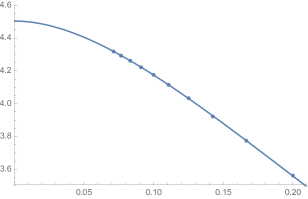
Figure 8: Effective scaling dimension, plotted against $1/L$, of the eigenvalues in $V_{0}$ (for $Q=\frac{1}{2}$) that correspond to the CFT scaling level $\phi_{3,1}\times\phi_{3,1}$, along with a polynomial extrapolation of order $9$.

Example 3.

We focus on the scaling level which corresponds to the eigenvalue of rank $i_{14}=16$ for $L=14$, i.e., line 16 in Table 1. Assume that the first 15 lines of the table have already been determined. We then try to determine $i_{13}$, which a priori can be any of the values not used in the first 15 lines: $i_{13}=15,17,18,19,\ldots$. To this end, plot the effective scaling dimensions (117) for $L=13,14$ against $1/L$ along with a linear fit in $1/L$, for all possible values of $i_{13}$. It is quickly seen that only the choice $i_{13}=16$ will lead to an exponent of the expected value $x_{\ell}\approx 5$. Fixing this choice, we next seek to determine $i_{12}$, which can take any of the unused values $i_{12}=15,16,18,19,\ldots$. Plot now the effective scaling dimensions for $L=12,13,14$ against $1/L$ along with a quadratic fit in $1/L$. This fit clearly singles out $i_{12}=19$ and narrows down the value of the exponent to $x_{\ell}\approx 4.5$. Going on in this way, including one by one the smaller sizes, and increasing the order of the fits, one determines all the ranks $i_{L}$ in line 16 of the table, down to the smallest size $L_{\rm min}=5$. The final fit, using all ten sizes $L=L_{\rm min},\ldots,L_{\rm max}$ and a polynomial extrapolation of order $9$ is shown in Figure 8. It leads to a very precise estimate $x_{\ell}\approx 4.50369$, which is in excellent agreement with the exact scaling dimension $4.50378\cdots$ of the field $\phi_{3,1}\times\phi_{3,1}$. Moreover, we can check that for the three smallest sizes, the eigenvalues with $(i_{5},i_{6},i_{7})=(11,14,16)$ all have lattice momentum $m=0$, so the CFT field must indeed have conformal spin $h-\bar{h}=0$.

The contents of Table 1 can be quickly summarised by saying that we have numerically observed within $V_{0}$ three different primaries,

$$\phi_{1,1}\times\phi_{1,1}\equiv I\,,\qquad\phi_{2,1}\times\phi_{2,1}\equiv\varepsilon\,,\qquad\phi_{3,1}\times\phi_{3,1}\equiv\varepsilon^{\prime}\,,$$ (119)

along with their corresponding Kac modules (where the generic Verma module of $\phi_{r,s}$ has been quotiented by one singular vector at level $rs$). More precisely:

• For the identity operator $I$ we have observed all descendents up to and including the total level $N\equiv n+\bar{n}=5$, and some of the descendents at level $6$. This operator is seen to be degenerate at level 1.

• For the energy operator $\varepsilon$ we have observed all descendents up to and including level $N=3$, and some of the descendents at level $4$. This operator is degenerate at level 2, as witnessed by the fact that we only observe a single state (and not $p(2)=2$ states) at level $(n,\bar{n})=(2,0)$.

• For the second energy operator $\varepsilon^{\prime}$ we have observed only the primary at level $N=0$, due to the high scaling dimension $x=4.503782\cdots$.

Table 2 gives the results of a similar investigation for the sector $V_{1}$. We here observe numerically two different primaries,

$$\phi_{1/2,0}\times\phi_{1/2,0}\equiv\sigma\,,\qquad\phi_{3/2,0}\times\phi_{3/2,0}\equiv\sigma^{\prime}\,,$$ (120)

along with their corresponding Verma modules. More precisely:

• For the magnetisation operator $\sigma$ we have observed all descendents up to and including the total level $N=3$, and some of the descendents at level $4$.

• For the second magnetisation operator $\sigma^{\prime}$ we have observed all descendents up to and including level $N=2$.

• We have not observed the expected third magnetisation operator, $\phi_{5/2,0}\times\phi_{5/2,0}$, due to its high scaling dimension $x=4.960593\cdots$.

Remark 9.

We stress that no degenerate states appear in these magnetisation operators, and accordingly their Verma modules are generic. This is in a nutshell why the determination of four-point functions in the bulk case is so difficult: the absence of degenerate states implies that we cannot write down differential equations satisfied by the correlation functions.

$V_{\ell,k,m}$	$(i_{5},i_{6},\ldots,i_{13})$									$x_{\ell}$		Identification
	5	6	7	8	9	10	11	12	13	Numerics	Exact	of scaling field
$V_{100}$	1	1	1	1	1	1	1	1	1	0.082745	0.082757	$\phi_{1/2,0}\times\phi_{1/2,0}\equiv\sigma$
$V_{101}$	2	2	2	2	2	2	2	2	2	1.08278	1.08276	$L_{-1}\sigma$
$V_{100}$	4	3	3	3	3	3	3	3	3	1.7091	1.7087	$\phi_{3/2,0}\times\phi_{3/2,0}\equiv\sigma^{\prime}$
$V_{102}$	3	4	4	4	4	4	4	4	4	2.0819	2.08276	$L_{-2}\sigma$
$V_{102}$	5	6	5	5	5	5	5	5	5	2.0830	2.0828	$L_{-2}\sigma$
$V_{100}$	6	7	6	6	6	6	6	6	6	2.08255	2.08276	$L_{-1}\bar{L}_{-1}\sigma$
$V_{101}$	7	8	8	9	8	8	7	7	7	2.704	2.079	$L_{-1}\sigma^{\prime}$
$V_{103}$	–	5	7	7	7	7	8	8	8	3.094	3.083	$L_{-3}\sigma$
$V_{103}$	–	9	9	10	10	9	9	9	9	3.072	3.083	$L_{-3}\sigma$
$V_{101}$	9	11	10	11	11	11	10	10	10	3.080	3.083	$L_{-2}\bar{L}_{-1}\sigma$
$V_{103}$	–	12	11	12	12	12	11	11	11	3.075	3.083	$L_{-3}\sigma$
$V_{101}$	12	14	14	14	13	14	13	12	12	3.081	3.083	$L_{-2}\bar{L}_{-1}\sigma$
$V_{104}$	–	–	–	8	9	10	12	13	13	4.078	4.083	$L_{-4}\sigma$
$V_{102}$	8	10	12	13	14	15	15	14	14	3.712	3.709	$L_{-2}\sigma^{\prime}$
$V_{100}$	11	15	17	17	16	17	16	16	15	3.69	3.71	$L_{-1}\bar{L}_{-1}\sigma^{\prime}$
$V_{102}$	15	17	18	20	21	18	18	19	16	3.69	3.71	$L_{-2}\sigma^{\prime}$
$V_{102}$	10	13	15	18	18	19	19	20	19	4.070	4.082	$L_{-3}\bar{L}_{-1}\sigma$
$V_{100}$	14	19	20	23	25	25	23	24	23	4.0841	4.0828	$L_{-2}\bar{L}_{-2}\sigma$
$V_{102}$	16	20	21	24	26	26	24	25	24	4.075	4.083	$L_{-3}\bar{L}_{-1}\sigma$
$V_{100}$	17	21	23	25	27	27	26	26	25	4.079	4.083	$L_{-2}\bar{L}_{-2}\sigma$

Table 2: Conformal spectrum in the sector $V_{1}$, for $Q=\frac{1}{2}$.

Finally, Table 3 shows our results for the sector $V_{2}$. We see here the beginning of the conformal towers of the primaries $\phi_{e,2}\times\phi_{e,-2}$ for $e=0,\frac{1}{2},1,\frac{3}{2},2$. As for $V_{1}$, there are no singular vectors in this case neither.

$V_{\ell,k,m}$	$(i_{5},i_{6},\ldots,i_{12})$								$x_{\ell}$		Identification
	5	6	7	8	9	10	11	12	Numerics	Exact	of scaling field
$V_{200}$	1	1	1	1	1	1	1	1	1.109570	1.109567	$\phi_{0,2}\times\phi_{0,-2}\equiv\phi_{0}$
$V_{211}$	2	2	2	2	2	2	2	2	1.31286	1.31281	$\phi_{1/2,2}\times\phi_{1/2,-2}\equiv\phi_{1/2}$
$V_{202}$	3	3	3	3	3	3	3	3	1.92257	1.92254	$\phi_{1,2}\times\phi_{1,-2}\equiv\phi_{1}$
$V_{201}$	5	4	4	4	4	4	4	4	2.1099	2.1096	$\bar{L}_{-1}\phi_{0}$
$V_{212}$	4	5	5	5	5	5	5	5	2.3117	2.3128	$\bar{L}_{-1}\phi_{1/2}$
$V_{210}$	7	7	6	6	6	6	6	6	2.31299	2.31281	$L_{-1}\phi_{1/2}$
$V_{203}$	–	8	8	7	7	7	7	7	2.914	2.923	$\bar{L}_{-1}\phi_{1}$
$V_{202}$	6	9	9	9	9	8	8	8	3.094	3.110	$\bar{L}_{-2}\phi_{0}$
$V_{213}$	–	10	11	11	10	10	10	9	2.9365	2.9388	$\phi_{3/2,2}\times\phi_{3/2,-2}\equiv\phi_{3/2}$
$V_{201}$	13	13	13	13	11	11	11	10	2.9228	2.9225	$L_{-1}\phi_{1}$
$V_{213}$	–	6	7	8	8	9	9	11	3.326	3.313	$\bar{L}_{-2}\phi_{1/2}$
$V_{200}$	9	11	12	15	12	12	12	12	3.1088	3.1096	$L_{-1}\bar{L}_{-1}\phi_{0}$
$V_{202}$	15	16	16	17	15	13	13	13	3.1098	3.1096	$\bar{L}_{-2}\phi_{0}$
$V_{211}$	10	12	14	16	16	14	14	14	3.308	3.313	$L_{-1}\bar{L}_{-1}\phi_{1/2}$
$V_{211}$	11	14	15	18	18	16	15	15	3.310	3.313	$L_{-2}\phi_{1/2}$
$V_{213}$	–	15	17	19	19	18	16	16	3.311	3.313	$\bar{L}_{-2}\phi_{1/2}$
$V_{211}$	17	21	20	20	21	21	18	17	3.3131	3.3128	$L_{-2}\phi_{1/2}$
$V_{204}$	–	–	–	12	14	17	17	18	3.907	3.922	$\bar{L}_{-2}\phi_{1}$
$V_{204}$	–	–	–	10	13	15	19	19	4.347	4.361	$\phi_{2,2}\times\phi_{2,-2}\equiv\phi_{2}$
$V_{212}$	8	17	19	22	24	27	30	31	4.296	4.313	$L_{-1}\bar{L}_{-2}\phi_{1/2}$

Table 3: Conformal spectrum in the sector $V_{2}$, for $Q=\frac{1}{2}$.

A.5.2 The special case $Q=4$

In Appendix B we show that the case $Q=4$ can be compared with an exact solution. It is therefore a particularly important benchmark for the numerical method. Moreover, it is well known that the $Q=4$ case is hampered by slow convergence, due to the logarithmic corrections produced by a marginally irrelevant operator. To make sure that our generic analysis applies in this case as well, we shall need the same kind of tables as above with this value of $Q$. They are obtained using the same methods as before, and are shown in Tables 4–6.

The precision of the extrapolated exponents $x_{\ell}$ suffers somewhat from the logarithmic corrections to scaling. But assuming that the operator content of the generic case carries over, the assignment of sector labels is nevertheless certain for the levels shown in the tables. To this end, it is particularly helpful that the observed exponent difference between a descendent operator and its corresponding primary is determined with considerably better precision than the exponents themselves.

This phenomenon is vividly illustrated in Table 4. For example, the primary $\varepsilon$ has the exact scaling dimension $\frac{1}{2}$, but the numerically measured exponent of $0.62$ is very imprecise. However, the corresponding measurements for the descendents at level $1$, $2$ and $3$ come out as $1.64$, $2.64$ (or $2.67$) and $3.63$ (or $3.60$), with the gaps being quite close to integers.

Similarly, the exponent of the primary $\varepsilon^{\prime}$ is measured as $2.35$ instead of the exact value of $2$. This is per se a catastrophic lack of precision—but it actually makes it easier to correctly identify the descendent $L_{-1}\varepsilon^{\prime}$, whose measured exponent comes out as $3.36$ with an almost perfect integer gap! Without this phenomenon one could easily have mixed up the numerical value $3.36$ with the other candidate exact value of $\frac{7}{2}$.

In a similar fashion we have the Tables 5–6 for the sectors $V_{1}$ and $V_{2}$, respectively. Note that the rank of eigenvalues whole momentum labels are fixed by analytic continuation—using the PT symmetry (116)—for small values of $L$ are shown as tiny numbers in the tables. In the previous Tables 1–3 (for $Q=\frac{1}{2}$) we have left blank such entries, although they can be determined in those cases as well.

$V_{\ell,k,m}$	$(i_{5},i_{6},\ldots,i_{13})$									$x_{\ell}$		Identification
	5	6	7	8	9	10	11	12	13	Numerics	Exact	of scaling field
$V_{000}$	1	1	1	1	1	1	1	1	1	0	0	$\phi_{1,1}\times\phi_{1,1}\equiv I$
$V_{000}$	2	2	2	2	2	2	2	2	2	0.619	0.5	$\phi_{2,1}\times\phi_{2,1}\equiv\varepsilon$
$V_{001}$	3	3	3	3	3	3	3	3	3	1.637	1.5	$L_{-1}\varepsilon$
$V_{002}$	4	4	4	4	4	4	4	4	4	2.0003	2	$L_{-2}I$
$V_{000}$	7	7	8	7	7	6	6	5	5	2.338	2	$\phi_{3,1}\times\phi_{3,1}\equiv\varepsilon^{\prime}$
$V_{002}$	5	5	5	5	5	5	5	6	6	2.646	2.5	$L_{-2}\varepsilon$
$V_{003}$	5	6	6	6	6	7	7	7	7	2.9994	3	$L_{-3}I$
$V_{000}$	6	8	9	8	8	8	8	8	8	2.659	2.5	$L_{-1}\bar{L}_{-1}\varepsilon$
$V_{003}$	4	6	7	9	9	9	9	9	9	3.620	3.5	$L_{-3}\varepsilon$
$V_{004}$	3	5	7	10	10	10	10	10	10	3.994	4	$L_{-4}I$
$V_{001}$	10	12	12	11	12	13	11	11	11	3.353	3	$L_{-1}\varepsilon^{\prime}$
$V_{003}$	9	11	11	12	13	14	12	12	12	3.603	3.5	$L_{-3}\varepsilon$
$V_{001}$	8	9	10	13	14	15	15	13	13	3.671	3.5	$L_{-2}\bar{L}_{-1}\varepsilon$

Table 4: Conformal spectrum in the sector $V_{0}$, for $Q=4$.

$V_{\ell,k,m}$	$(i_{5},i_{6},\ldots,i_{12})$								$x_{\ell}$		Identification
	5	6	7	8	9	10	11	12	Numerics	Exact	of scaling field
$V_{100}$	1	1	1	1	1	1	1	1	0.133	0.125	$\phi_{1/2,0}\times\phi_{1/2,0}\equiv\sigma$
$V_{101}$	2	2	2	2	2	2	2	2	1.138	1.125	$L_{-1}\sigma$
$V_{100}$	3	3	3	3	3	3	3	3	1.212	1.125	$\phi_{3/2,0}\times\phi_{3/2,0}\equiv\sigma^{\prime}$
$V_{102}$	4	4	4	4	4	4	4	4	2.132	2.125	$L_{-2}\sigma$
$V_{102}$	5	6	5	5	5	5	5	5	2.126	2.125	$L_{-2}\sigma$
$V_{100}$	7	8	7	7	7	6	6	6	2.149	2.125	$L_{-1}\bar{L}_{-1}\sigma$
$V_{101}$	6	7	6	6	6	7	7	7	2.218	2.125	$L_{-1}\sigma^{\prime}$
$V_{103}$	4	5	8	8	8	8	8	8	3.107	3.125	$L_{-3}\sigma$
$V_{103}$	8	9	9	10	9	9	9	9	3.116	3.125	$L_{-3}\sigma$
$V_{102}$	8	10	10	11	11	10	10	10	3.202	3.125	$L_{-2}\sigma^{\prime}$
$V_{101}$	12	13	14	12	12	12	11	11	3.121	3.083	$L_{-2}\bar{L}_{-1}\sigma$
$V_{103}$	9	11	12	13	13	13	12	12	3.131	3.125	$L_{-3}\sigma$
$V_{101}$	10	12	13	14	14	14	13	13	3.145	3.125	$L_{-2}\bar{L}_{-1}\sigma$
$V_{100}$	11	14	15	17	15	16	15	14	3.225	3.125	$L_{-1}\bar{L}_{-1}\sigma^{\prime}$
$V_{102}$	13	16	16	18	16	17	16	15	3.236	3.125	$L_{-2}\sigma^{\prime}$
$V_{104}$	2	4	8	9	10	11	14	16	4.114	4.125	$L_{-4}\sigma$
$V_{100}$	15	17	17	19	19	18	17	17	3.37	3.125	$\phi_{5/2,0}\times\phi_{5/2,0}\equiv\sigma^{\prime\prime}$
$V_{104}$	6	10	11	15	17	19	19	18	4.07	4.125	$L_{-4}\sigma$
$V_{105}$	1	2	4	8	10	15	18	19	5.23	5.125	$L_{-5}\sigma$
$V_{103}$	5	9	11	16	18	20	20	20	4.16	4.125	$L_{-3}\sigma^{\prime}$

Table 5: Conformal spectrum in the sector $V_{1}$, for $Q=4$.

$V_{\ell,k,m}$	$(i_{5},i_{6},\ldots,i_{11})$							$x_{\ell}$		Identification
	5	6	7	8	9	10	11	Numerics	Exact	of scaling field
$V_{200}$	1	1	1	1	1	1	1	1.83	2	$\phi_{0,2}\times\phi_{0,-2}\equiv\phi_{0}$
$V_{211}$	2	2	2	2	2	2	2	1.97	2.125	$\phi_{1/2,2}\times\phi_{1/2,-2}\equiv\phi_{1/2}$
$V_{202}$	3	3	3	3	3	3	3	2.38	2.5	$\phi_{1,2}\times\phi_{1,-2}\equiv\phi_{1}$
$V_{201}$	5	4	4	4	4	4	4	2.82	3	$\bar{L}_{-1}\phi_{0}$
$V_{212}$	4	5	5	5	5	5	5	2.96	3.125	$\bar{L}_{-1}\phi_{1/2}$
$V_{210}$	7	6	6	6	6	6	6	2.96	3.125	$L_{-1}\phi_{1/2}$
$V_{213}$	8	10	9	8	7	7	7	3.06	3.125	$\phi_{3/2,2}\times\phi_{3/2,-2}\equiv\phi_{3/2}$
$V_{203}$	6	8	7	7	8	8	8	3.36	3.5	$\bar{L}_{-1}\phi_{1}$
$V_{201}$	10	11	12	11	9	9	9	3.36	3.5	$L_{-1}\phi_{1}$
$V_{202}$	6	9	10	10	10	10	10	3.84	4	$\bar{L}_{-2}\phi_{0}$
$V_{213}$	4	7	8	9	11	11	11	4.01	4.125	$\bar{L}_{-2}\phi_{1/2}$
$V_{200}$	11	13	14	15	12	12	12	3.82	4	$L_{-1}\bar{L}_{-1}\phi_{0}$
$V_{211}$	9	12	13	16	13	13	14	3.96	4.125	$L_{-1}\bar{L}_{-1}\phi_{1/2}$
$V_{202}$	14	16	15	17	16	14	13	3.80	4	$\bar{L}_{-2}\phi_{0}$

Table 6: Conformal spectrum in the sector $V_{2}$, for $Q=4$.

A.6 Ising model

Finally we discuss the case of a unitary minimal model, namely the Ising model ($Q=2$). A special case of the first of the identities (9) then reads [14]

$$G_{aaaa}=\langle\sigma_{1}\sigma_{2}\sigma_{3}\sigma_{4}\rangle=P_{aaaa}+P_{aabb}+P_{abba}+P_{abab}\,,$$ (121)

where we have used the short-hand notation $\sigma_{i}=Q\delta_{S_{i},+}-1$ for the usual FK spin operator ${\cal O}_{a}(\sigma_{i})$ (5) and $S_{i}=\pm$ are the four Ising spins. Inserting the definition of $\sigma_{i}$, we can express $G_{aaaa}$ in terms of the probabilities $P(S_{1},S_{2},S_{3},S_{4})$ of having fixed values of the $S_{i}$:

$$\langle\sigma_{1}\sigma_{2}\sigma_{3}\sigma_{4}\rangle=\sum_{S_{1},S_{2},S_{3},S_{4}=\pm}(-1)^{\sum_{i=1}^{4}\delta(S_{i},+)}P(S_{1},S_{2},S_{3},S_{4})\,.$$ (122)

It is straightforward to write a transfer matrix that computes the probabilities $P(S_{1},S_{2},S_{3},S_{4})$ in the Ising spin representation, by simply projecting on the required values of $S_{i}$ at the position of each operator. Doing this we have verified the above identity to 4000 decimal places for various systems. Since this relates very non-trivially the probabilities in the FK representation—whose computation is intricate, as we have seen in section A.1—to those in the Ising representation, this provides a strong test of the correctness of our transfer matrix setup.

We can now compute $G_{aaaa}$ at larger sizes and analyse it in terms of the eigenvalues of the Ising spin transfer matrix. Since two spin operators are inserted simultaneously, the propagating states should only be those of the $\mathbb{Z}_{2}$-even sector, and we have verified that this is indeed the case. j Added: Note that the $\mathbb{Z}_{2}$-even sector is the simple module $\mathcal{X}_{0,i}=\overline{\mathcal{W}}_{0,\mathfrak{q}^{2}=i}-\mathcal{W}_{3,1}+\cdots$ which is the ‘top’ corresponding to the leftmost diagram in Figure 9 (see [27] for details). In the conformal limit we expect the propagating states to be the identity, $\phi_{1,1}\times\phi_{1,1}\equiv I$, and the energy operator, $\phi_{2,1}\times\phi_{2,1}\equiv\varepsilon$.

We postpone the further discussion of these results to Appendix B. However, to refine the analysis and parallel the discussion given above for generic $Q$ and the case $Q=4$, we shall again need to establish the precise correspondence between the finite-size and the conformal spectra. This is done in Table 7, where the rank of eigenvalues now refer only to the $\mathbb{Z}_{2}$-even part of the spin representation (and not to a sector of the full FK transfer matrix spectrum).

Note that the spin transfer matrix does not contain sufficient information to attribute a momentum label to the eigenvalues. However, since the Ising spectrum is included in the FK spectrum we can still rely on the sizes $L=5,6,7$ to assign momentum labels to each level.

$V_{\ell,k,m}$	$(i_{5},i_{6},\ldots,i_{20})$																$x_{\ell}$		Identification
	5	6	7	8	9	10	11	12	13	14	15	16	17	18	19	20	Numerics	Exact	of scaling field
$V_{000}$	1	1	1	1	1	1	1	1	1	1	1	1	1	1	1	1	0	0	$\phi_{1,1}\times\phi_{1,1}\equiv I$
$V_{000}$	2	2	2	2	2	2	2	2	2	2	2	2	2	2	2	2	$1+10^{-12}$	1	$\phi_{2,1}\times\phi_{2,1}\equiv\varepsilon$
$V_{001},V_{002}$	3	3	3	3	3	3	3	3	3	3	3	3	3	3	3	3	2.0000002	2	$L_{-1}\varepsilon,L_{-2}I$
$V_{002},V_{003}$	4	4	4	4	4	4	4	4	4	4	4	4	4	4	4	4	3.000003	3	$L_{-2}\varepsilon,L_{-3}I$
$V_{000}$	5	5	6	5	5	5	5	5	5	5	5	5	5	5	5	5	3.0000004	3	$L_{-1}\bar{L}_{-1}\varepsilon$
$V_{003},V_{004}$	3	4	5	6	6	6	6	6	6	6	6	6	6	6	6	6	3.9995	4	$L_{-3}\varepsilon,L_{-4}I$
$V_{001}$	6	6	7	7	8	8	8	7	7	7	7	7	7	7	7	7	4.000003	4	$L_{-2}\bar{L}_{-1}\varepsilon$
$V_{000}$	7	8	9	9	9	9	10	10	9	8	8	8	8	8	8	8	4.0000002	4	$L_{-2}\bar{L}_{-2}I$
$V_{005}$	2	3	4	6	7	7	7	8	8	9	9	9	9	9	9	9	4.99994	5	$L_{-5}I$
$V_{005}$	5	6	8	8	10	10	11	11	12	11	11	10	10	10	10	10	4.9999	5	$L_{-5}I$
$V_{000}$	–	7	9	10	12	12	12	12	13	13	12	12	12	11	11	11	5.00002	5	$L_{-2}\bar{L}_{-2}\varepsilon$
$V_{004},V_{001}$	8	9	11	12	13	13	15	14	14	14	15	13	13	13	12	12	5.000002	5	$L_{-4}\varepsilon,L_{-3}\bar{L}_{-2}I$
$V_{006}$	–	2	3	4	6	7	9	9	10	10	10	11	11	12	13	13	6.002	6	$L_{-6}I$
$V_{006}$	3	5	7	8	11	11	13	13	15	15	16	16	15	15	15	14	5.999	6	$L_{-6}I$
$V_{007}$	–	1	2	3	4	6	7	9	11	12	13	14	14	14	14	15	7.0004	7	$L_{-7}I$
$V_{006}$	6	7	10	11	14	14	16	16	18	17	17	17	18	17	16	16	5.9998	6	$L_{-6}I$
$V_{005}$	7	9	12	14	16	16	17	17	19	19	19	18	19	19	18	17	5.9999	6	$L_{-5}\varepsilon$
$V_{000}$	–	10	13	15	20	19	20	19	20	20	21	20	21	20	19	18	5.99997	6	$L_{-3}\bar{L}_{-3}I$
$V_{007}$	–	–	1	2	3	4	6	8	10	12	14	15	16	16	17	19	7.98	8	$L_{-7}\varepsilon$
$V_{003},V_{002}$	9	11	15	16	21	21	23	21	22	21	23	21	22	22	21	20	6.000003	6	$L_{-4}\bar{L}_{-1}\varepsilon,L_{-4}\bar{L}_{-2}I$
$V_{007}$	–	3	6	7	10	11	14	15	16	16	18	19	20	21	23	21	7.0002	7	$L_{-7}I$
$V_{009}$	–	–	–	1	2	3	4	6	8	10	13	15	17	18	20	22	8.9	9	$L_{-9}I$
$V_{009}$	–	–	–	–	1	2	3	4	6	9	10	14	16	18	22	23	9.85	10	$L_{-9}\varepsilon$
$V_{007}$	4	6	9	11	15	15	18	18	21	22	24	24	24	23	24	24	6.999	7	$L_{-7}I$
$V_{006}$	6	8	11	14	18	18	22	23	24	23	25	25	25	25	26	25	6.99995	7	$L_{-6}\varepsilon$
$V_{???}$	–	–	–	13	17	17	21	22	23	24	26	26	27	26	27	26	6.9993	7
$V_{008}$	–	–	3	6	8	10	13	15	17	18	20	22	23	24	25	27	7.9992	8	$L_{-8}I$
$V_{006}$	8	10	14	17	22	23	27	26	29	28	28	27	29	28	28	28	6.9997	7	$L_{-6}\varepsilon$
$V_{???}$	9	11	16	18	24	24	29	28	31	29	30	29	31	30	30	29	6.9996	7

Table 7: Conformal spectrum in the $\mathbb{Z}_{2}$-even sector for the Ising model ($Q=2$). The rank $i_{k}$ of the eigenvalues refer to this sector only, and not to the full spectrum of the corresponding FK model.

Doing this we encounter an interesting phenomenon: In some cases a given eigenvalue corresponds to two different momentum labels. For instance, the 3rd eigenvalue belongs simultaneously to $V_{001}$ and $V_{002}$ for $L=5,6,7$; the 4th eigenvalue belongs to $V_{002}$ and $V_{003}$ for $L=6,7$; and the 7th eigenvalue belongs to $V_{001}$ and $V_{003}$ for $L=7$. We recall that we count here only distinct eigenvalues, so statements of this type mean that the eigenvalue is degenerate (in addition to the usual degeneracy coming from the sign of the momentum), with different momentum identifications for each of the degenerate states. The momentum labels $m$ assigned to the lowest-rank eigenvalues for $L=5,6,7$ are shown in Table 8.

Rank	$L$
$i_{k}$	5	6	7
1	0	0	0
2	0	0	0
3	$1,2$	$1,2$	$1,2$
4	2	$2,3$	$2,3$
5	0	0	3
6	1	1	0
7	0	0	$1,3$
8	1	0	2
9	2	$1,2$	0
10		0	1
11		$2,3$	$1,3$
12		$1,2$	2
13		0	0
14		0	1
15			$2,3$

Table 8: Momentum labels $m$ (modulo $L$) for the first 15 eigenvalues in the $\mathbb{Z}_{2}$-even sector for the Ising model ($Q=2$). We have not been able to identify the labels $i_{L}$ for line 17 of the table.

With all these ingredients, a close inspection of Table 7 reveals that we observe precisely the minimal characters $\chi_{r,s}(q)$ corresponding to the identity and energy operators, namely $\widetilde{\chi}_{r,s}(q)\equiv q^{-h_{r,s}+c/24}\chi_{r,s}(q)$ with the expansions

$$(r,s)=(1,1) : 1+q^{2}+q^{3}+2q^{4}+2q^{5}+3q^{6}+\cdots\,,$$ (123a)

$$(r,s)=(2,1) : 1+q+q^{2}+q^{3}+2q^{4}+2q^{5}+\cdots\,.$$ (123b)

A.7 Practical remarks

A.7.1 Diagonalisation of $T$

Our diagonalisation of the transfer matrix $T$ is based on its decomposition (10) as a product of sparse matrices. Indeed, the elementary operators ${\sf J}_{i}$ and ${\sf D}_{i}$ have at most one non-zero entry per column. It is therefore feasible to compute $w=Tv$—i.e., the action of $T$ on a vector of weights $v$—without ever storing $T$ and working only on its non-zero entries. It follows that it is highly efficient to diagonalise $T$ by iterative methods that require only the operator $w=Tv$ and not $T$ itself. Among such methods, we have found that the Arnoldi method is well suited for our situation, where $T$ is a non-symmetric real matrix.

We have used the C++ interface for the Fortran library Arpack [58] for producing both eigenvalues and eigenvectors, in cases where standard numerical precision (16 digits) is sufficient. This applies in particular to the scalar product method of section A.2. For the more direct method of section A.1, a considerably higher numerical precision is needed. To this end we have used the CLN package [59] (again written in C++) that performs floating point operators to any desired numerical precision. We are greatly indebted to Christian R. Scullard who has provided a pure C++ version of Arpack with templates that are compatible with CLN; this is unpublished work, but it has been described in recent publications on a different subject [60, 61, 62].

A.7.2 Boundary conditions

In the first method (see section 4.3.1) we compute the probabilities $P_{\cal P}$ corresponding to FK cluster correlation functions on the cylinder (see Figure 1). As described in section A.1 this is done in practice by expressing the probability as the the ratio of partition functions $W_{\cal P}$ on finitely long cylinders, where free boundary conditions have been imposed at a distance $M$ from the insertion points of the cluster operators.

To ensure that the result does not depend on $M$, the latter much be chosen large enough. Let $d$ denote the number of decimal digits in the desired numerical precision. Let $\Lambda_{I}$ and $\Lambda_{\varepsilon}$ be the largest and next-largest eigenvalues of $T$ within the sector $V_{0}$; it is easy to compute their values beforehand. We now claim that we must chose $M$ so that $(\Lambda_{\varepsilon}/\Lambda_{I})^{M}\leq 10^{-d}$.

As the notation shows, these two eigenvalues are associated, throughout the critical regime $0\leq Q\leq 4$, with the scaling levels that determine respectively the identity $I$ and the energy operator $\varepsilon$. It should be noticed that $\Lambda_{\varepsilon}$ thus defined is most definitely not the next-largest eigenvalue of $T$, if we take into account all sectors. This latter eigenvalue would rather be $\Lambda_{\sigma}$, the largest eigenvalue within the sector $V_{1}$, associated with the scaling level of the leading order parameter operator $\sigma$, which has the smallest non-zero scaling dimension in the CFT. In other words, we have $\Lambda_{I}>\Lambda_{\sigma}>\Lambda_{\varepsilon}$. The point of the claim made above is then that outside the region $t\in[t_{1},t_{2}]$ of the cylinder (see Section A.1 for notations) that contains the operator insertions, there are no constraints enforcing the propagation of clusters. This implies that the dominant decaying mode is given by the ratio $\Lambda_{\varepsilon}/\Lambda_{I}$, as can easily be checked by direct inspection of the numerically computed probabilities.

A.7.3 Attainable sizes

The largest sizes $L$ attainable in the numerical work are essentially limited by the exponentially growing dimensions of the corresponding transfer matrices. For the first method (see section 4.3.1) there is however an additional complication, since we do not obtain the amplitudes $A_{i}$ directly but acquire them by solving the linear system (53).

Suppose first that there are $K$ eigenvalues coupling to $P_{\cal P}$, and call $\Lambda_{\rm max}$ and $\Lambda_{\rm min}$ the largest and smallest of those. If all computations are done to $d$ decimal digits, and we wish to obtain the final values of the amplitudes to $d_{0}$ digits, then we must chose $d$ large enough that $(\Lambda_{\rm min}/\Lambda_{\rm max})^{K}>10^{d_{0}-d}$. Indeed, we will need the separation between operators to take the values $l=1,2,\ldots,K$ in order to have enough equations to solve the linear system for $A_{i}$. And assuming all $A_{i}$ to be of the order unity, the smallest term on the right-hand side of (53) should not be below the level of numerical precision.

Similar considerations can be made for the case where $K$ is so large that we are unable (or do not want) to determine all the amplitudes. In that case, we truncate the sum in (53) at some $i_{\rm max}$, and provide $i_{\rm max}$ different values of $l$. Since the formula is no longer exact, we must make sure to use it in the proper asymptotic regime. We therefore take $l=i_{\rm min},i_{\rm min}+1,\ldots,i_{\rm max}$ for some suitable large $i_{\rm min}$. In practice we have chosen $i_{\rm min}=100$ and repeated the computation for a slightly higher value (e.g., $i_{\rm min}=120$), in order to check that the $A_{i}$ were unchanged to the desired numerical precision.

In our largest computations, for $L=7$, we determined more than 500 amplitudes in this way. This computation needed as much as $d=4000$ digits of numerical precision and required the work of $\sim 100$ computers simultaneously for a period of $\sim 3$ months. See section 5.2.2 for further details on this computation.

For the second scalar product method (see section 4.3.2) it was enough to work with standard double precision ($d=16$ digits). This method is altogether more efficient and could be done up to $L=11$ in a much more reasonable time (at most a few days on a single computer).

A.7.4 Jordan blocks

With the first method it is possible to determine the Jordan block structure of correlation functions, by using a fit of the form (54). To do this in practice requires some reasonable prior knowledge about where to look for the Jordan blocks, and about their expected order $r_{i}$. The analytical understanding of indecomposability in the Temperley-Lieb algebra has grown steadily over recent years, including in the affine TL case [26], so the search for Jordan blocks is certainly not devoid of any guidance. However, one can also take a more naive numerical approach to the problem.

Imagine that we are interested in some specific value $Q=Q_{0}$, where indecomposability is known to occur. Consider a correlation function $P_{\cal P}$ for which we have previously established, for generic $Q$, which transfer matrix sectors $V_{\ell,k,m}$ occur with a non-zero amplitude. At the non-generic $Q_{0}$, some of the eigenvalues from different sectors will collide, as can be seen by explicit diagonalisation using the methods of section A.4 (or predicted analytically). The number of eigenvalues that collide at a given value $\Lambda_{i}$ is a natural guess for the largest possible rank $r_{i}$ of the Jordan block corresponding to the generalised amplitude (54). Trying the corresponding Ansatz for different values of $i_{\rm min}$ (see above), we can examine whether the amplitudes are consistently determined (and non-zero) and arrive at a quantitative understanding of the Jordan block structure.

A.7.5 Extrapolation of amplitudes

Whichever method is used for obtaining the eigenvalue amplitudes $A_{i}$ on the cylinder, the results need to be extrapolated to infinite size ($L\to\infty$) in order to be compared with predictions of conformal field theory. We shall see in Appendix B that in many cases the finite-size results are quite far away from their CFT limits, more often than not by a factor in the range 2–5. Obtaining reliable extrapolations is important, in particular because we only possess rather small sizes ($L\leq 11$). Moreover, most amplitudes exhibit mod 2 parity effects, so that even and odd $L$ must be treated separately.

Some guidance can be taken from our results for the Ising model where larger sizes can be obtained ($L\leq 16$). We find the following method to provide quite accurate results. First we produce finite-size results with $\frac{2a}{L}$ equal to or close to a constant, typically $\frac{1}{2}$. Since it turns out that some amplitudes vanish exactly, by symmetry reasons, for $\frac{2a}{L}=\frac{1}{2}$ precisely, we often take $2a=(L-1)/2$ for odd $L$, and $2a=(L-2)/2$ for even $L$. These results are then corrected by a conformal factor, namely the powers of $\sin\frac{2\pi a}{L}$ appearing in (35). Finally, we extrapolate the corrected results, separately for odd and even $L$, by fitting all available data against a polynomial in $1/L$ (or in some cases leaving out the first or first few data points). The reliability of the extrapolation can then be estimated by comparing the two parities, which are expected to give identical results.

A.8 The split-attach algebra

The scalar product method described in section 4.3.2 and appendix A.2 requires us to find the left eigenvectors of $T$. One way to attain this is to take the transpose of the right eigenvectors of the transposed matrix $T^{\rm t}$.

The scalar product method described in section 4.3.2 and appendix A.2 requires us to find the left eigenvectors of $T$. One way to attain this is to take the transpose of the right eigenvectors of the transposed matrix $T^{\rm t}$.

In the join-detach algebra for the FK cluster model, $T$ acts on basis states which are set partitions of $L$ points. The basic building block of the sparse matrix factorisation scheme (10) is the action of the elementary join and detach operators, ${\sf J}_{i}$ and ${\sf D}_{i}$, on these states. If this was presented in explicit matrix form, it would of course be trivial to take the transpose of the corresponding matrices. The point is, however, that when we use an iterative diagonalisation scheme (such as the Arnoldi method; see section A.7.1), it is inefficient to represent ${\sf J}_{i}$ and ${\sf D}_{i}$ as explicit matrices. Rather, we just need to provide their action on any state: for any in-state $v_{\rm in}$, the definition of ${\sf J}_{i}$ (or ${\sf D}_{i}$) in terms of set partitions provides the corresponding out-state $v_{\rm out}={\sf J}_{i}v_{\rm in}$ (or ${\sf D}_{i}v_{\rm in}$). To treat the transpose in a similar setting means that we should instead answer the question: given $v_{\rm out}$, what are the possible $v_{\rm in}$ that could lead to it (and with which transition weights)?

We therefore formally define the split operator ${\sf S}_{i}={\sf J}_{i}^{\rm t}$ and the attach operator ${\sf A}_{i}={\sf D}_{i}^{\rm t}$ as the transpose of the join and detach operator, respectively, and provide now their transition elements in terms of the basis states.

A.8.1 Without marked clusters

We first consider the analogue of the usual join-detach algebra, that is, without any marked clusters.

The operator ${\sf S}_{i}$ performs a split between sites $i$ and $i+1$. In particular, ${\sf S}_{i}$ is zero on states in which sites $i$ and $i+1$ are not connected (i.e., in the same block of the set partition). If the two sites are connected, ${\sf S}_{i}$ acts by breaking up the block containing $i$ and $i+1$ in all possible ways. To be precise, assume the block consist of $k\geq 2$ points, ordered cyclically: $i_{1}<i_{2}<\cdots<i_{k}<i_{1}$ (the inequalities being considered modulo $L$), with $i_{1}=i$ and $i_{2}=i+1$. Place one “separator” between $i_{1}$ and $i_{2}$. Place a second separator at the position of any of the above inequalities, i.e., between $i_{\ell}$ and $i_{\ell+1}$ for any $\ell=1,2\ldots,k$, with the subscripts considered mod $k$. Note that this includes the case where the two separators are at identical positions. Then break up the block by cutting it at the positions of the two separators. This produces the $k$ possible out-states of ${\sf S}_{i}$, which each occur with transition weight $1$. Note that the block is being broken into precisely two pieces in the $k-1$ cases where the two separators are different, whereas nothing happens (i.e., ${\sf S}_{i}$ acts as the identity) in the remaining case where the separators coincide.

The operator ${\sf A}_{i}$ attaches a singleton at site $i$ to certain other blocks of the set partition, as we now describe. In particular, ${\sf A}_{i}$ is zero on states in which site $i$ is not a singleton. If $i$ is an singleton, ${\sf A}_{i}$ leaves the state unchanged with weight $Q$, and connects $i$ to any other “visible” block in the set partition with weight $1$. To determine whether a block is visible by $i$, draw the set partition as a hypergraph with vertex set $1,2,\ldots,L$ embedded in the half-infinite cylinder (concretely, in Figure 1 this would be the part of the cylinder situated to the left of the current time slice, with the vertices on the slice). If a block is adjacent to the face where $i$ resides, the block is said to be visible. Another, less formal way to state the same, is that we connect $i$ to any block that is not nested within another block, seen from the position of $i$.

It is straightforward (albeit somewhat laborious) to verify that the split-detach algebra thus defined satisfies the algebraic relations which are the transpose of those defining the join-detach algebra:

$${\sf S}_{i}^{2} = {\sf S}_{i}\,,$$ (124a)

$${\sf A}_{i}^{2} = A{\sf D}_{i}\,,$$ (124b)

$${\sf S}_{i}{\sf A}_{j}{\sf S}_{i} = {\sf S}_{i}\mbox{ for }j=i,i+1\,,$$ (124c)

$${\sf A}_{i}{\sf S}_{j}{\sf A}_{i} = {\sf A}_{i}\mbox{ for }j=i-1,i\,.$$ (124d)

A.8.2 With marked clusters

We now provide the definition of the split-attach algebra in the representation with marked clusters having a fixed spin label. This is analogous to section A.2.

The split operator ${\sf S}_{i}$ acts as zero, unless sites $i$ and $i+1$ belong to the same block (which can be unmarked or marked). Otherwise:

• If $i$ and $i+1$ belong to the same unmarked block, ${\sf S}_{i}$ leaves the block unchanged or splits it into two unmarked blocks, as before, with a total of $k$ possibilities for a block of size $k$.

• If $i$ and $i+1$ belong to the same marked block, ${\sf S}_{i}$ leaves the block unchanged or splits it into two blocks, of which one is unmarked and the other keeps the same mark as the original block. Both choices for which of the two blocks should carry the mark are realised.

The attach operator ${\sf A}_{i}$ acts as zero, unless site $i$ is an unmarked singleton. Otherwise:

• With weight $Q$, the operator ${\sf A}_{i}$ leaves the singleton block at $i$ unchanged and unmarked.

• With weight $1$, it marks site $i$ by each possible colour of the mark which is used in none of the other blocks in the partition.

• With weight $1$, it attaches site $i$ to each of its visible blocks (which can be marked or unmarked).

The two first rules cover the cases where the corresponding detach operation is trivial, in the sence that ${\sf D}_{i}$ would turn a (marked or unmarked) singleton into an unmarked singleton. The third rule covers the non-trivial case, where the corresponding detach operation acts on a (marked or unmarked) block of size $\geq 2$.

With these modifications one can again check that the defining relations (124) are satisfied, but within the larger representation that allows clusters to be marked.

Appendix B Basic checks

In this appendix we check our general method for computing the amplitudes $A_{i}$ against a series of exact results. First we discuss the easy case of two-point functions and quantify the conformal content of the lattice spin operator. Next we compare our results for the $s$-channel spectrum of four-point functions against exact solutions for $Q=2$, $Q=4$, and the limit $Q\to 0$.

B.1 Lattice observables and scaling fields

As discussed in the main text, one of the basic difficulties in our problem is that lattice observables correspond, in the scaling limit, to combinations of scaling fields weighed with appropriate powers of the cut-off. The question we want to investigate briefly here is how this might affect the measurement of amplitudes.

According to (8), the two-point function of the lattice spin operator becomes, in the geometrical formulation, proportional to the probability that two points belong to the same cluster. The leading dimension controlling the large distance behavior of this probability is $h_{1/2,0}$ and thus we expect, in the scaling limit, to have on the cylinder

$$P_{aa}\;\xrightarrow{\rm\,scaling}\;\left({\xi\over(1-\xi)^{2}}{\bar{\xi}\over(1-\bar{\xi})^{2}}\right)^{h_{1/2,0}}\,.$$ (125)

We have here used the same notation (33) as for the four-point function, so $w_{1}=ia$, $w_{3}=i(a+x)+l$, and $w_{13}=-ix-l$. As before, we set $\xi=e^{-2\pi(l+ix)/L}$, and the above dependence on $\xi,\bar{\xi}$ follows from a reasoning similar to the one leading to (4.1). We find numerically that only the sector $F_{0,-1}$ contributes, with

$$F_{0,-1}=\frac{q^{-c/24}\bar{q}^{-c/24}}{P(q)P(\bar{q})}\sum_{e\in\mathbb{Z}}q^{h_{e+1/2,0}}\bar{q}^{h_{e+1/2,0}}\,.$$ (126)

As is usually the case in lattice models, the order operator on the lattice is not purely represented by a conformal field of weight $(h_{1/2,0},h_{1/2,0})$. In general, one expects instead that this field is only the first in a sum of the type

$${\cal O}_{a}(\sigma_{i})\sim\sum_{e\in\mathbb{Z}}A_{e}\epsilon^{2h_{e+1/2,0}}\Phi_{e+1/2,0}(z)\Phi_{e+1/2,0}(\bar{z})+\hbox{descendants}\,,$$ (127)

where $z,\bar{z}$ are the complex coordinates corresponding to $\sigma_{i}$, we have introduced the notation $\Phi_{r,s}$ for conformal chiral fields with weight $h_{rs}$, and $\epsilon$ stands for the lattice cutoff ($\epsilon$ was set equal to unity so far). In the limit where $L,l\to\infty$ (that is, $L/\epsilon,l/\epsilon\to\infty$ if $L,l$ are measured in units of length) the contributions of the excited (higher) spin fields will scale away. For finite values of the parameters, they are unavoidably there. Note that

$$h_{3/2,0}-h_{1/2,0}={m+1\over 2m}\,.$$ (128)

This is larger for small values of $m$, i.e., smaller values of $Q$: therefore, the closer we will get to $Q=0$, the faster these contributions will decrease with $\epsilon$ ($\epsilon/L$ on the cylinder).

We do not know how the $Q$-dependent amplitudes $A_{e}$ in (127) behave a priori, but we have studied numerically the two-point function in order to understand the amount of “mixing” of the order operator with the leading correction at weight $h_{3/2,0}$. We have checked that this mixing is small and decreases significantly with increasing $L$.

As an example, we give here results for $Q=3/2$—a case for which $m$ is irrational, and all operators in the spectrum can be uniquely identified. The dimension of the order parameter is $h_{1/2,0}=0.0583892$, and by (125) the two-point function in the conformal limit expands as

$$P_{aa}^{\rm scaling}\propto\xi^{h_{1/2,0}}\bar{\xi}^{h_{1/2,0}}\left(1+0.116778(\xi+\bar{\xi})+0.0136372\xi\bar{\xi}+0.0652078(\xi^{2}+\bar{\xi}^{2})+\ldots\right)\,,$$ (129)

where all numerical constants have been given to six-digit precision. The leading terms at momentum $h-\bar{h}=1$ and $h-\bar{h}=2$ are easily identified as the ground states of the corresponding momentum sectors. With no knowledge of the possible mixing with the term $\xi^{h_{3/2,0}}\bar{\xi}^{h_{3/2,0}}$ one would look for the $\xi\bar{\xi}$ term in (129) in the lattice data as the contribution of the first excited state in the sector at vanishing momentum, but a careful analysis of the amplitudes as well as the scaling dimensions shows this is not what happens. On the lattice, the two point function contains, in addition to the terms in (129), a term in the bracket proportional to $(\xi\bar{\xi})^{h_{3/2,0}-h_{1/2,0}}$. This follows from (127), which leads to

$$P_{aa}^{\rm lattice}\propto{1\over|z|^{4h_{1/2,0}}}\left[1+\left({A_{1}\over A_{0}}\right)^{2}\left({\epsilon\over|z|}\right)^{4(h_{3/2,0}-h_{1/2,0})}+\ldots\right]\,,$$ (130)

and, after mapping on the cylinder, to

$$P_{aa}^{\rm lattice} \propto \left({2\pi\over L}\right)^{4h_{1/2,0}}\left[\left({\xi\over(1-\xi)^{2}}\right)^{h_{1/2,0}}\left({\bar{\xi}\over(1-\bar{\xi})^{2}}\right)^{h_{1/2,0}}\right.$$ (131)

$$+ \left.\left({A_{1}\over A_{0}}\right)^{2}\left({2\pi\epsilon\over L}\right)^{4(h_{3/2,0}-h_{1/2,0})}\left({\xi\over(1-\xi)^{2}}\right)^{h_{3/2,0}}\left({\bar{\xi}\over(1-\bar{\xi})^{2}}\right)^{h_{3/2,0}}+\ldots\right]\,.$$

The amplitude ratio $A_{1}/A_{0}$ is non-universal, but, for a given lattice, it is a fixed quantity. The term $L^{-4(h_{3/2,0}-h_{1/2,0})}$ goes to zero as $L$ goes to infinity, guaranteeing the disappearance of the unwanted terms in this limit. The question is how much this might affect the results for $L$ finite.

Measurement of the amplitudes—or rather the ratio with respect to the leading term—gives the following results:

$$\begin{array}[]{c|llll}L&\xi+\bar{\xi}&\xi\bar{\xi}&\xi^{2}+\bar{\xi}^{2}&(h_{3/2,0},h_{3/2,0})\\ \hline\cr 5&0.1009697881&0.004693387836&0.05633421252&-0.0007594762012\\ 6&0.1044947727&0.006252504965&0.05534757764&-0.0006074838333\\ 7&0.1070768500&0.007528362715&0.05578623767&-0.0004817486169\\ 8&0.1089775943&0.008549110109&0.05665273685&-0.0003834115301\\ 9&0.1103983091&0.009361639062&0.05759817991&-0.0003078006915\\ 10&0.1114793562&0.010010585922&0.05849501339&-0.0002497183860\\ 11&0.1123166454&0.010532656068&0.05930089355&-0.0002048250690\\ 12&0.1129759889&0.010956414072&0.06000781281&-0.0001698028289\\ \infty&0.11679&0.13644&0.06519&<10^{-6}\\ {\rm CFT}&0.116778&0.0136372&0.0652078&0\\ \hline\cr\end{array}$$ (143)

The extrapolation to $L\to\infty$ was made via a polynomial of order 7 in $1/L$, using all data points, since there are no discernable parity effects in this case. We observe that on one hand the expected ratios converge to their conformal values to a very good precision (4 or 5 digits). On the other, the one that is not expected—corresponding to the coupling to $(h_{3/2,0},h_{3/2,0})$—decreases fast, and converges to a value close to zero. This example shows that one can obtain fine extrapolations, even though for the sizes considered in this paper (and the value $Q=3/2$ taken here) the mixing of the field $(h_{3/2,0},h_{3/2,0})$ with the order parameter has a rather large relative coefficient of the order of $10^{-2}$.

B.2 The case $Q=2$

We now consider the case $Q=2$ (and later $Q=4$) to check the consistency of our approach, and assess the quality of convergence of the amplitudes in the four-point functions. While in general, the geometrical probabilities cannot be expressed in terms of simple four-point functions in rational CFTs, the situation is better for these two values of $Q$. This has to do with the relationship [14] between correlation functions of spins in the Potts model and the geometrical objects, see eq. (9). We stress that for $Q$ arbitrary, the left-hand sides of these equations are only formally defined: it is in fact the right-hand sides that give them a meaning. In the $Q=2$ case the first relation (9a) reads simply

$$G_{aaaa}=P_{aaaa}+P_{aabb}+P_{abba}+P_{abab}\,,\quad\mbox{for }Q=2\,.$$ (144)

On the other hand, recall from (7) that

$$G_{aaaa}=\langle\prod_{i=1}^{4}(Q\delta_{\sigma_{i},a}-1)\rangle$$ (145)

As discussed in A.6, for $Q=2$, the order parameter $Q\delta_{\sigma_{i},a}-1$ coincides with the Ising spins $S_{i}=\pm 1$, so this four-point function is nothing but the four-point function of the spin operator in the Ising model [63]

$$\langle\sigma(z_{1})\sigma(z_{2})\sigma(z_{3})\sigma(z_{4})\rangle = {1\over 2}\left|{z_{13}z_{24}\over z_{12}z_{23}z_{34}z_{41}}\right|^{1/4}\left(\left|1+\sqrt{1-z}\right|+\left|1-\sqrt{1-z}\right|\right)$$ (146)

$$= {1\over 2}|z_{13}|^{-1/4}|z_{24}|^{-1/4}{1\over|z(1-z)|^{1/4}}\left(\left|1+\sqrt{1-z}\right|+\left|1-\sqrt{1-z}\right|\right)\,.$$

We also recall the structure constant $C_{\sigma\sigma\epsilon}={1\over 2}$, where $\epsilon$ denotes the energy operator; the latter appears as the non-trivial part of the scaling limit of $S_{i}S_{i+1}$. The four-point function (146) involves two conformal blocks, corresponding to the fusion channels $\sigma\sigma\sim 1$ and $\sigma\sigma\sim\epsilon$. Expanding the function $\mathrm{G}$ as in (28) gives then

$$|z|^{1/4}\mathrm{G}(z,\bar{z})=1+{1\over 4}z^{1/2}\bar{z}^{1/2}+{1\over 16}(z^{1/2}\bar{z}^{3/2}+z^{3/2}\bar{z}^{1/2})+{1\over 64}z^{3/2}\bar{z}^{3/2}+{1\over 64}(z^{2}+\bar{z}^{2})+\ldots\,.$$ (147)

The normalised correlation function on the lattice should then be

$$1+s^{2}(\xi\bar{\xi})^{1/2}+(s^{2}-s^{4})(\xi\bar{\xi})^{1/2}(\xi+\bar{\xi})+{s^{4}\over 4}(\xi^{2}+\bar{\xi}^{2})+(s^{2}-2s^{4}+s^{6})(\xi\bar{\xi})^{3/2}+\frac{s^{8}}{16}(\xi\bar{\xi})^{2}+\ldots\,,$$ (148)

where $s=\sin{2\pi a\over L}$, and the extra terms arise from the conformal mapping as in (4.1).

B.2.1 Reduction from the generic case

We first checked—by computing the four-spin correlation function numerically for the ordinary (spin representation) Ising model on the cylinder—that the identity (144) holds exactly in finite size; details are given in section A.6. This computation is certainly a rather stringent test of the program that determines the $P_{a_{1},a_{2},a_{3},a_{4}}$ numerically. Note that the (large) set of eigenvalues that contribute to the geometrical correlations for generic values of $Q$ reduces drastically—as expected—when we consider the combination (144). In algebraic terms, generically irreducible representations of the Jones algebra become reducible, and a complex structure of submodules of the relevant $\overline{\mathcal{W}}_{j,z^{2}}$ develops. It turns out that only two simple quotients contribute to the Ising model: $\mathcal{X}_{0,i}$ and $\mathcal{X}_{0,-1}$, which are obtained as the the ‘tops’ of chains of modules according to the diagrams in Figure 9 (for a detailed discussion of the emergence of simple modules of the Jones algebra describing minimal models when $\mathfrak{q}$ is a root of unity, see [27]).

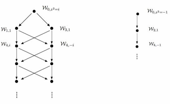
Figure 9: The simple modules $\mathcal{X}_{0,i}$ and $\mathcal{X}_{0,-1}$ are the tops of these two diagrams representing the structure of the standard modules for $\mathfrak{q}=e^{i\pi/4}$.

The continuum limit of the simple modules of the Jones algebra is fully expressed in terms of irreducible modules $\mathsf{X}_{r,s}$ of the Virasoro algebra

$$\mathcal{X}_{0,i} \mapsto \mathsf{X}_{1,1}\otimes\overline{\mathsf{X}}_{1,1}\bigoplus\mathsf{X}_{21}\otimes\overline{\mathsf{X}}_{2,1}=\mathsf{X}_{h=0}\otimes\overline{\mathsf{X}}_{h=0}\bigoplus\mathsf{X}_{h=1/2}\otimes\overline{\mathsf{X}}_{h=1/2}\,,$$ (149a)

$$\mathcal{X}_{0,-1} \mapsto 2\,\mathsf{X}_{12}\otimes\overline{\mathsf{X}}_{12}=2\,\mathsf{X}_{h=1/16}\otimes\overline{\mathsf{X}}_{h=1/16}\,,$$ (149b)

where the factor 2 indicates that, in fact, the representation splits into two isomorphic direct summands for the subalgebra generated by $e_{i}$ and $u^{2}$, and $\mathsf{X}_{r,s}$ denotes the irreducible Virasoro module with conformal weight $h_{rs}$ (and, e.g., character given by the well-known Rocha-Caridi formula [64]).

We checked that the combination (144) receives contributions only from the tops in the diagrams in Figure 9 , which corresponds, in the continuum limit, to the required channels of the minimal Ising model. Note however that individual probabilities in (144), unlike their sum, do involve contributions outside the simple representations.

B.2.2 Numerical checks of the amplitudes

We now turn to the question of the convergence of the amplitudes measured on the lattice. Surprisingly, it seems this question has not been investigated much in the past (see [65] for early work). Since the Ising model is much easier to handle numerically than the general FK cluster model, we can study in this case much larger sizes (up to $L_{\rm max}=16$), and explore in particular the nature of the convergence of the coefficients in the expansion (148).

We present in the following Figures 10–11 two different ways of handling the data. First, we consider the case where $a$ is changed as $L$ increases. For definiteness we consider $2a={L\over 2}$ when $L$ is even and $2a={L-1\over 2}$ when $L$ is odd. In both cases, $\sin{2\pi a\over L}\rightarrow 1$ as $L\rightarrow\infty$, but we should of course expect even/odd parity effects in $L$ because of the different choices of $2a$.

A priori the aim would be to compute the amplitude ratios, with respect to the ground state amplitude, corresponding to the five last terms in (148), namely the contributions to $G_{aaaa}$ of $\epsilon$, $(L_{-1}+\bar{L}_{-1})\epsilon$, $T+\bar{T}$, $\bar{L}_{-1}L_{-1}\epsilon$, and $T\bar{T}$, respectively. However it turns out that $(L_{-1}+\bar{L}_{-1})\epsilon$ and $T+\bar{T}$ correspond to eigenvalues that are exactly degenerate in finite size, so the corresponding contributions cannot be disentangeled. We thus list the amplitude ratios in (148) that we can access numerically along with their corresponding analytical predictions:

$$\epsilon : s^{2}$$ (150a)

$$(L_{-1}+\bar{L}_{-1})\epsilon+(T+\bar{T}) : 2\left(s^{2}-\frac{3}{4}s^{4}\right)$$ (150b)

$$\bar{L}_{-1}L_{-1}\epsilon : s^{2}-2s^{4}+s^{6}$$ (150c)

$$T\bar{T} : \frac{s^{8}}{16}$$ (150d)

The four panels of Figure 10 show the corresponding amplitudes ratios, where in each case we have divided the ratio by the expected analytical result just given. It is seen that in each case the result tends to $1$ after extrapolation, thus confirming the whole analysis.

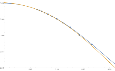
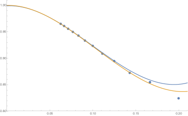
(a)                                                                      (b)

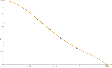
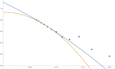
(c)                                                                      (d)

Figure 10: Measures of the first four amplitude ratios in $G_{aaaa}$ for the Ising model, divided by the expected analytical results. The respective panels show the contributions from (a) the energy operator $\epsilon$, (b) its first descendent $(L_{-1}+\bar{L}_{-1})\epsilon$ along with the stress tensor $T+\bar{T}$, (c) its second descendent $\bar{L}_{-1}L_{-1}\epsilon$, and (d) the quantity $T\bar{T}$. All data is shown against $1/L$. The extrapolations for even and odd $L$ are shown respectively as blue and orange curves.

A number of remarks can be made about Figure 10. First, the extrapolations have to be carried out using some amount of common sense. In some cases the obvious non-monotonicity of the finite-size results (panel d) makes it clear that one should leave out the first few points from the fits. In other cases, (panel c) including all points in a high-order polynomial fit leads to the best results. Second, the comparison between fits through even and odd sizes appears to be a good measure for the “error bar” on the extrapolated value. Third, there is a tendency for the finite-size effects to grow as one goes to higher descendents. Thus, if we were limited to smaller sizes—such as $L_{\rm max}=11$, as would be the case for the FK cluster model at generic values of $Q$—it should be expected that the last data point might very well be off the true extrapolated value by a factor of 2 or more.

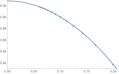
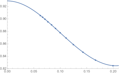
(a)                                                                      (b)

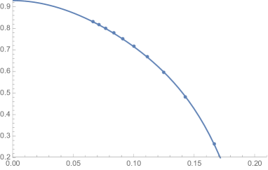
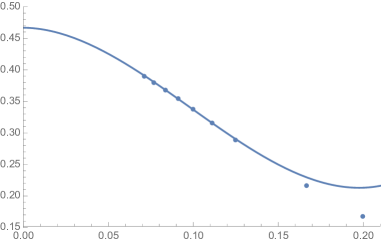
(c)                                                                      (d)

Figure 11: Same as Figure 10, but for a fixed distance $2a=2$ between each pair of operators. The panels are as in Figure 10. The extrapolations, shown as blue curves, now uses sizes $L$ of both parities.

It is also interesting to study what happens when $a$ is fixed while $L$ is increased. In this case, one does not expect the amplitude ratios to converge to the four-point CFT values reported in (150), since the latter require $a,L\gg 1$ (in units of the lattice spacing) with fixed value of the ratio $\frac{a}{L}$ (and hence $s$ fixed). To illustrate this, we consider for instance the case of $2a=2$ fixed, with $L$ increasing—note that we do not expect parity effects using this protocol. To make the analysis comparable to the one above, we again divide the ratio by the CFT predictions (150). The results are shown in Figure 11, to be compared with the previous Figure 10. Clearly the convergence is no longer towards one. It is however remarkable that the numerical data still appear to converge to a finite value. For the energy operator and its first two descendents (panels a, b, c) we get fine extrapolations to the values $0.9292$, $0.9289$ and $0.9292$ respectively, which are all compatible among themselves. For $T\bar{T}$ the extrapolations are more problematic, but still appear to converge to a finite value $\simeq 0.53$, which definitely appears to be different from the previous one.

We are not sure whether these values can be interpreted within CFT—neither whether the observed convergence is real or only apparent. Repeating the computations for $2a=3$, a similar extrapolation gives the consistent values $0.9686$ and $0.9680$ for the energy field and its first descendent, whereas $T\bar{T}$ gives another value $\simeq 0.71$.

B.3 The case $Q=4$

As pointed out in [1], the Potts model at $Q=4$ is particularly interesting, since in this case all geometrical correlation functions can be expressed in terms of spin correlation functions. This provides analytical results for all the $P_{abcd}$, and thus provides a simple benchmark against which to test our approach. There is however a drawback to this idea: numerics for the Potts model at $Q=4$ are known to be affected by stronger than usual corrections to scaling due to the presence of a marginal operator. As a result, convergence to the expected amplitudes appears to be slower than for other values of $Q$, especially small ones.

In any case, we start by observing that the Potts model partition function, can be expressed in the continuum limit as the sum [7, 66],

$$Z_{\rm Potts~{}Q=4}=\sum_{n\in\mathbb{Z}}F_{2n,1}-{1\over 2}F_{2n+1,1}+{3\over 2}F_{2n,-1}\,,$$ (151)

where the generating functions are obtained by taking the limit $m\to\infty$ of our general result (46)

$$F_{j,1} = {1\over\eta\bar{\eta}}\sum_{k\in\mathbb{Z}}q^{(j+k)^{2}/4}\bar{q}^{(j-k)^{2}/4}\,,$$ (152a)

$$F_{j,-1} = {1\over\eta\bar{\eta}}\sum_{k\in\mathbb{Z}}q^{(j+k+1/2)^{2}/4}\bar{q}^{(j-k-1/2)^{2}/4}\,.$$ (152b)

In contrast with the case of generic $Q$ [7], we see that only a very small subset of the $F_{j,e^{2i\pi p/M}}$ generating functions contribute. This corresponds to the fact—which we checked explicitly in finite size, and which has a simple representation theoretic interpretation; see below—that of all the usual Jones algebra modules, only those corresponding to $z^{2}=\pm 1$ play a role at $Q=4$.

B.3.1 Exact results via the Ashkin-Teller model

After these preliminaries, we now consider four-point functions per se. In [1], some of the probabilities at $Q=4$ are given based on results in [14], combined with the careful reading of a paper by Al.B. Zamolodchikov [67]. Calling $\tau_{1},\tau_{2}$ the two spins of the Ashkin-Teller model, we introduce, following [67], the four quantities

$$R_{1} = \langle\tau_{1}\tau_{2}\tau_{2}\tau_{1}\rangle\,,$$ (153a)

$$R_{2} = \langle\tau_{1}\tau_{1}\tau_{2}\tau_{2}\rangle\,,$$ (153b)

$$R_{3} = \langle\tau_{1}\tau_{2}\tau_{1}\tau_{2}\rangle\,,$$ (153c)

$$G = \langle\tau_{1}\tau_{1}\tau_{1}\tau_{1}\rangle\,;$$ (153d)

note that $G$ here must not be confused with $\mathrm{G}$ in (23). It is then expected that

$$P_{aabb} \propto G+R_{2}-R_{1}-R_{3}\,,$$ (154a)

$$P_{aaaa} \propto -G+R_{1}+R_{2}+R_{3}\,,$$ (154b)

$$P_{abab}-P_{abba} \propto R_{1}-R_{3}\,.$$ (154c)

The quantities on the right-hand side are then calculated in [67]. We introduce first

$$F_{0}(z)\equiv[z(1-z)]^{-1/8}\theta_{3}^{-1}(\mathrm{q})\,,$$ (155)

where $z=\frac{z_{12}z_{34}}{z_{13}z_{24}}$ as usual. We shall also need the Jacobi theta functions

$$\theta_{3}(\mathrm{q}) = \sum_{-\infty}^{\infty}\mathrm{q}^{n^{2}}\,,$$ (156a)

$$\theta_{2}(\mathrm{q}) = \sum_{-\infty}^{\infty}\mathrm{q}^{(n+1/2)^{2}}\,.$$ (156b)

These two functions are used to define $\mathrm{q}(z)$ implicitly via

$$z\equiv{\theta_{2}^{4}(\mathrm{q})\over\theta^{4}_{3}(\mathrm{q})}$$ (157)

Note that the function $\mathrm{q}(z)$ is analytic in $z$:

$$\mathrm{q}(z)=\frac{z}{16}+\frac{z^{2}}{32}+\frac{21z^{3}}{1024}+\frac{31z^{4}}{2048}+\frac{6257z^{5}}{524288}+\frac{10293z^{6}}{1048576}+\frac{279025z^{7}}{33554432}+\frac{483127z^{8}}{67108864}+\ldots\,.$$ (158)

We then set

$$G = F_{0}\bar{F}_{0}\sum_{m,n=-\infty}^{\infty}\mathrm{q}^{(\beta_{+}m+\beta_{-}n)^{2}}\bar{\mathrm{q}}^{(\beta_{+}m-\beta_{-}n)^{2}}\,,$$ (159a)

$$R_{1} = F_{0}\bar{F}_{0}\sum_{m,n=-\infty}^{\infty}\mathrm{q}^{(\beta_{+}m+\beta_{-}(n+1/2))^{2}}\bar{\mathrm{q}}^{(\beta_{+}m-\beta_{-}(n+1/2))^{2}}\,,$$ (159b)

$$R_{2} = F_{0}\bar{F}_{0}\sum_{m,n=-\infty}^{\infty}(-1)^{m}\mathrm{q}^{(\beta_{+}m+\beta_{-}n)^{2}}\bar{\mathrm{q}}^{(\beta_{+}m-\beta_{-}n)^{2}}\,,$$ (159c)

$$R_{3} = F_{0}\bar{F}_{0}\sum_{m,n=-\infty}^{\infty}(-1)^{m}\mathrm{q}^{(\beta_{+}m+\beta_{-}(n+1/2))^{2}}\bar{\mathrm{q}}^{(\beta_{+}m-\beta_{-}(n+1/2))^{2}}\,.$$ (159d)

Finally we choose

$$\beta_{+}=1\,,$$ (160a)

$$\beta_{-}={1\over 2}\,.$$ (160b)

The claim is then that the $z,\bar{z}$ dependent part of the four-point function (the function $\mathrm{G}$ of section 4.1) is given by corresponding combinations of the functions $G$ and $R_{i}$. So for instance

$$P_{aabb}\propto|z_{12}z_{34}|^{-1/4}\mathrm{G}_{aabb}(z,\bar{z})\,,$$ (161)

with

$$\mathrm{G}_{aabb}(z,\bar{z}) = G+R_{2}-R_{1}-R_{3}$$ (162)

$$= 2F_{0}\bar{F}_{0}\left(\sum_{m,n=-\infty}^{\infty}\mathrm{q}^{(2m+n/2)^{2}}\bar{\mathrm{q}}^{(2m-n/2)^{2}}-\mathrm{q}^{(2m+n/2+1/4)^{2}}\bar{\mathrm{q}}^{(2m-n/2-1/4)^{2}}\right)\,.$$

What we must do then is to expand the combinations (159) in powers of $z$. This gives expressions of the form

$$(z\bar{z})^{-1/8}\sum_{\Delta\bar{\Delta}}z^{\Delta}\bar{z}^{\bar{\Delta}}\,.$$ (163)

The point is that the set of weights $(\Delta,\bar{\Delta})$ is the set of conformal weights appearing in the s-channel expansion of the four point function. (It is not necessarily the set of primary fields, as the exact result does not distinguish between primaries and descendents. Hence our use of the notation $\Delta$ is slightly abusive when compared with the general case.) This must be the same set as the set of conformal weights contributing to the lattice observable. Hence, we must compare the sets occurring in (159) with the sets determined directly. These sets can be determined numerically, as for $Q$ generic, and are found to be:

$$\hbox{Spec~{}}P_{aabb} \subset \hbox{Spec~{}}\mathcal{W}_{0,1}/\mathcal{W}_{1,1}+\hbox{Spec~{}}\mathcal{W}_{0,-1}+\hbox{Spec~{}}\mathcal{W}_{2,1}/\mathcal{W}_{3,1}+\ldots\,,$$ (164a)

$$\hbox{Spec~{}}P_{aaaa} \subset \hbox{Spec~{}}\mathcal{W}_{0,-1}+\hbox{Spec~{}}\mathcal{W}_{2,1}/\mathcal{W}_{3,1}+\ldots\,,$$ (164b)

$$\hbox{Spec~{}}(P_{abab}-P_{abba}) \subset \hbox{Spec~{}}\mathcal{W}_{2,-1}+\ldots\,,$$ (164c)

$$\hbox{Spec~{}}(P_{abab}+P_{abba}) \subset \hbox{Spec~{}}\mathcal{W}_{2,1}/\mathcal{W}_{3,1}+\ldots\,.$$ (164d)

Here the quotients of modules have a direct meaning in terms of subtracting eigenvalues common to various sectors in finite size. Like for other non-generic values of $\mathfrak{q}$, the modules contributing to the probabilities are no longer irreducible, and the $Q=4$ results correspond to taking the simple irreducible tops. Indeed we find in general that $\hbox{Spec~{}}\mathcal{W}_{2k+1,1}\subset\hbox{Spec~{}}\mathcal{W}_{2k,1}$ for $k=1,2,\ldots$.

We have moreover established numerically that $\hbox{Spec~{}}(P_{abab}-P_{abba})$ does not contain $\hbox{Spec~{}}\mathcal{W}_{4,-1}$, which would otherwise have been a viable candidate in view of symmetries and the results for generic $Q$. For these reasons we conjecture that the complete result generalising (164) should in fact read:

$$\hbox{Spec~{}}P_{aabb} = \hbox{Spec~{}}\mathcal{W}_{0,1}/\mathcal{W}_{1,1}+\hbox{Spec~{}}\mathcal{W}_{0,-1}+\sum_{k\geq 1}\hbox{Spec~{}}\mathcal{W}_{2k,1}/\mathcal{W}_{2k+1,1}\,,$$ (165a)

$$\hbox{Spec~{}}P_{aaaa} = \hbox{Spec~{}}\mathcal{W}_{0,-1}+\sum_{k\geq 1}\hbox{Spec~{}}\mathcal{W}_{2k,1}/\mathcal{W}_{2k+1,1}\,,$$ (165b)

$$\hbox{Spec~{}}(P_{abab}-P_{abba}) = \hbox{Spec~{}}\mathcal{W}_{2,-1}\,,$$ (165c)

$$\hbox{Spec~{}}(P_{abab}+P_{abba}) = \sum_{k\geq 1}\hbox{Spec~{}}\mathcal{W}_{2k,1}/\mathcal{W}_{2k+1,1}+\,.$$ (165d)

B.3.2 Probability $P_{aaaa}$

First we consider $P_{aaaa}$. The spectrum predicted from the decomposition in (164) is

$$(q\bar{q})^{1/24}F_{0,-1} = 2q^{1/16}\bar{q}^{1/16}\left(1+q+\bar{q}+(q\bar{q})^{1/2}+q\bar{q}+\ldots\right)\,,$$ (166a)

$$(q\bar{q})^{1/24}\left(F_{2,1}-F_{3,1}+\ldots\right) = q\bar{q}+q^{1/4}\bar{q}^{9/4}+q^{9/4}\bar{q}^{1/4}+\ldots\,.$$ (166b)

Corresponding to this we find

$$-G+R_{1}+R_{2}+R_{3} = (z\bar{z})^{-1/8}\left(\sqrt{2}z^{1/16}\bar{z}^{1/16}+{1\over 16\sqrt{2}}(z^{1/16}\bar{z}^{17/16}+z^{17/16}\bar{z}^{1/16})+{1\over 8\sqrt{2}}(z\bar{z})^{9/16}+\ldots\right.$$ (167)

$$\left.-{1\over 128}z\bar{z}-{1\over 512}(z^{1/4}\bar{z}^{9/4}+z^{9/4}\bar{z}^{1/4})+\ldots\right)\,,$$

and thus, after mapping to the cylinder

$$P_{aaaa} \propto (\xi\bar{\xi})^{1/16}+{\cos^{2}{2\pi a\over L}\over 4\sqrt{2}}(\xi\bar{\xi})^{1/16}(\xi+\bar{\xi})+{\sin^{2}{2\pi a\over L}\over 2\sqrt{2}}(\xi\bar{\xi})^{9/16}+\ldots$$ (168)

$$-{(4\sin^{2}{2\pi a\over L})^{15/8}\over 128\sqrt{2}}\xi\bar{\xi}-{(4\sin^{2}{2\pi a\over L})^{19/8}\over 512\sqrt{2}}(\xi\bar{\xi})^{1/4}(\xi^{2}+\bar{\xi}^{2})+\ldots\,,$$

where we recall that

$$\xi=e^{-2\pi(l+ix)/L}\,,\quad\bar{\xi}=e^{-2\pi(l-ix)/L}\,.$$ (169)

The first and third terms in this expression are associated with the largest eigenvalue in $F_{0,-1}$ at zero momentum (this is denoted $V_{100}$ in section A.4). The second term also belongs to $F_{0,-1}$, but at non-zero momentum (namely $V_{101}$). Finally, the fourth and fifth terms are the leading ones in $F_{2,1}$ (in respective momentum sectors $V_{200}$ and $V_{202}$). To associate these terms to definite eigenvalues, for each size $L$, requires going through the detailed analysis of section A.5. We moreover note that one has to be careful in the comparison, since on the lattice we do not individually observe the amplitudes of conjugate terms, such as the two terms in $(\xi\bar{\xi})^{1/16}(\xi+\bar{\xi})$, since they correspond to the same eigenvalue. Therefore, to make the comparison we must divide the numerically observed amplitude by two in such cases (cf. remark 6)—this has been done tacitly below and in subsequent similar cases. This leads to the following results for the second to fifth terms in (168):

$$\begin{array}[]{ll|lllll}L&&(\xi\bar{\xi})^{1/16}(\xi+\bar{\xi})&(\xi\bar{\xi})^{9/16}&\xi\bar{\xi}&(\xi\bar{\xi})^{1/4}(\xi^{2}+\bar{\xi}^{2})\\ \hline\cr 5&{\rm lattice}&0.01025716807&0.2499038005&-0.1702401995&-0.05899812501\\ &{\rm CFT}&0.01688067229&0.3197920460&-0.0615759664&-0.02928111207\\ &{\rm ratio}&0.6076&0.7815&2.7647&2.0149\\ \hline\cr 7&{\rm lattice}&0.005692994702&0.2821337922&-0.1820689962&-0.06496561673\\ &{\rm CFT}&0.008753198131&0.3360469943&-0.0675747438&-0.03294025194\\ &{\rm ratio}&0.6504&0.8396&2.6943&1.9722\\ \hline\cr 9&{\rm lattice}&0.003595596367&0.2949643343&-0.1820598325&-0.06747242144\\ &{\rm CFT}&0.005330469599&0.3428924513&-0.0701787272&-0.03455627732\\ &{\rm ratio}&0.6745&0.8602&2.5942&1.9525\\ \hline\cr\end{array}$$ (180)

We see that the first two columns come out satisfactorily, and the ratios can be rather convincingly extrapolated to a number close to one, despite of the small number of sizes. For the higher-order terms (the last two columns of the table) the convergence is definitely slower, but still goes in the right direction. We have already seen (witness Figure 10 in the Ising case) that ratios of the order of $2$ at small sizes ($L\leq 9$ here) are not uncommon, and it is quite plausible that also these columns could be extrapolated to one, provided one could obtain a few more sizes. In conclusion, the test of $P_{aaaa}$ is fully compatible with the exact results.

B.3.3 Probability $P_{aabb}$

We next consider the probability $P_{aabb}$ of a pair of “short” clusters. The spectrum predicted from the decomposition in (164) is

$$(q\bar{q})^{1/24}F_{0,-1} = 2q^{1/16}\bar{q}^{1/16}\left(1+q+\bar{q}+(q\bar{q})^{1/2}+q\bar{q}+\ldots\right)\,,$$ (181)

$$(q\bar{q})^{1/24}\left(F_{0,1}-F_{1,1}+F_{2,1}-F_{3,1}+\ldots\right) = 1+(q\bar{q})^{1/4}+(q\bar{q})^{1/4}(q+\bar{q})+q\bar{q}+(q\bar{q})^{1/4}(q^{2}+\bar{q}^{2})+\ldots\,.$$

Correspondingly, we find

$$G-R_{1}+R_{2}-R_{3} = (z\bar{z})^{-1/8}\left(-\sqrt{2}(z\bar{z})^{1/16}-{1\over 16\sqrt{2}}(z\bar{z})^{1/16}(z+\bar{z})+\ldots\right.$$ (182)

$$+ \left.1+{1\over 2}(z\bar{z})^{1/4}+{1\over 16}(z\bar{z})^{1/4}(z+\bar{z})+\ldots\right)\,,$$

and thus

$$P_{aabb} \propto -\sqrt{2}(\xi\bar{\xi})^{1/16}+\ldots$$ (183)

$$+ 1+{(4\sin^{2}{2\pi a\over L})^{3/8}\over 2}(\xi\bar{\xi})^{1/4}+\ldots\,.$$

The first term is the leading eigenvalue in $F_{0,-1}$, corresponding in finite size to the largest eigenvalue in $V_{100}$. The second and third terms are the two leading eigenvalues in $\bar{F}_{0,1}$, corresponding to the two largest eigenvalues in $V_{000}$. The comparison with numerics—presented in the by now familiar format—here comes out as:

$$\begin{array}[]{ll|ll}L&&(\xi\bar{\xi})^{1/16}&(\xi\bar{\xi})^{1/4}\\ \hline\cr 5&{\rm lattice}&-1.342154491&0.6006793776\\ &{\rm CFT}&-1.414213562&0.8098363105\\ &{\rm ratio}&0.9490&0.7417\\ \hline\cr 7&{\rm lattice}&-1.400211084&0.7065845314\\ &{\rm CFT}&-1.414213562&0.8250340627\\ &{\rm ratio}&0.9901&0.8564\\ \hline\cr 9&{\rm lattice}&-1.431374714&0.7598690826\\ &{\rm CFT}&-1.414213562&0.8312967743\\ &{\rm ratio}&1.0121&0.9141\\ \hline\cr\end{array}$$ (194)

It again appears convincing that the ratios will converge to one, i.e., that the numerical results confirm the analytical ones.

B.3.4 The combination $P_{abab}-P_{abba}$

As a last example we discuss antisymmetric combination $P_{abab}-P_{abba}$ of the probabilities of having two “long” propagating clusters, as shown in Figure 2.

It is easy to expand the spectrum of exponents arising from (164) on the one hand: the first few terms are

$$(q\bar{q})^{1/24}F_{2,-1}=(q\bar{q})^{9/16}(q+\bar{q}+q^{2}+\bar{q}^{2}+2q\bar{q}+\ldots)+(q\bar{q})^{1/16}(q^{3}+\bar{q}^{3}+\ldots)\,.$$

The powers of $q,\bar{q}$ on the right-hand side are expected to be exactly the exponents appearing in the sum (163). Using the foregoing discussion and the expressions of $R_{1},R_{3}$, we can on the other hand identify these exponents by performing a direct expansion whose first few terms are:

$$R_{1}-R_{3}={(z\bar{z})^{-1/8}\over 128\sqrt{2}}\left\{(z\bar{z})^{9/16}\left(z+\bar{z}+{25\over 32}(z^{2}+\bar{z}^{2})+{9\over 16}z\bar{z}+\ldots\right)+(z\bar{z})^{1/16}\left({1\over 16}(z^{3}+\bar{z}^{3})+\ldots\right)\right\}\,.$$

This plays the role of the function $\mathrm{G}$ in our general discussion (4.1). It is easy to check that the two sets agree. Moreover, we have also checked that there is no gap in the spectrum, that is, all exponents predicted from the generating function (164) are indeed present with non-zero coupling constant.

To check the numerical values of the amplitudes, we need as usual to map the four-point function on the cylinder. We find the first few terms

$$P_{abab}-P_{abba} \propto (\xi\bar{\xi})^{9/16}(\xi+\bar{\xi})+\left[{9\over 4}-{9\sin^{2}{2\pi a\over L}\over 4}\right](\xi\bar{\xi})^{25/16}$$ (195)

$$+ \left[{25\over 8}-{25\over 8}\sin^{2}{2\pi a\over L}\right](\xi\bar{\xi})^{9/16}(\xi^{2}+\bar{\xi}^{2})+{\sin^{2}{2\pi a\over L}\over 4}(\xi\bar{\xi})^{1/16}(\xi^{3}+\bar{\xi}^{3})+\ldots)\,.$$

The first term corresponds to the lowest eigenvalue in the $F_{2,-1}$ sector with conformal spin $h-\bar{h}=1$, originating from $V_{211}$ in finite size. The second and third term correspond to the leading eigenvalue with $h-\bar{h}=0$ (resp. $h-\bar{h}=2$), originating from $V_{210}$ (resp. $V_{212}$)—note that since the scaling dimension $h+\bar{h}=\frac{25}{8}$ is the same for these two terms their ordering in the finite-size data cannot be guessed straightaway, and one has to make use of the lattice momentum to reveal the correct conformal spin. Finally, the fourth term corresponds to the lowest eigenvalue in the sector with $h-\bar{h}=3$—we notice that this state is not present for $L=5$, since this size is yet too small to accommodate the high value of the momentum. The numerical results for the last three terms being discussed (taking ratios with respect to the first term) now run as follows:

$$\begin{array}[]{ll|lll}L&&(\xi\bar{\xi})^{25/16}&(\xi\bar{\xi})^{9/16}(\xi^{2}+\bar{\xi}^{2})&(\xi\bar{\xi})^{1/16}(\xi^{3}+\bar{\xi}^{3})\\ \hline\cr 5&{\rm lattice}&0.05719383440&0.2474873290&0\\ &{\rm CFT}&0.10742794066&0.2984109462&0\\ &{\rm ratio}&0.5324&0.8294&\\ \hline\cr 7&{\rm lattice}&0.03267744359&0.1238111030&0.1246090804\\ &{\rm CFT}&0.05570501180&0.1547361439&0.2376211084\\ &{\rm ratio}&0.5866&0.8001&0.5244\\ \hline\cr 9&{\rm lattice}&0.02135602073&0.07680979880&0.1355927174\\ &{\rm CFT}&0.03392290080&0.09423028002&0.2424615776\\ &{\rm ratio}&0.6295&0.8151&0.5592\\ \hline\cr\end{array}$$ (206)

Finally, observe that the Kac parametrisation

$$h_{rs}={[(m+1)r-ms]^{2}-1\over 4m(m+1)}$$ (207)

becomes, in the limit $m\to\infty$, $h_{rs}={(r-s)^{2}\over 4}$. The exponents appearing in the various Ashkin-Teller correlators are thus in agreement with the spectra conjectured in [1]

$$G : ~{}~{}\mathcal{S}_{\mathbb{Z},2\mathbb{Z},}$$

$$R_{1} : ~{}~{}\mathcal{S}_{\mathbb{Z}+{1\over 2},2\mathbb{Z},}$$

$$R_{2} : ~{}~{}\mathcal{S}_{\mathbb{Z},2\mathbb{Z}}$$

$$R_{3} : ~{}~{}\mathcal{S}_{\mathbb{Z}+{1\over 2},2\mathbb{Z}}$$ (208)

after the switch of $r,s$ labels mentioned earlier in remark 5.

B.4 The case $Q=0$

The case $Q=0$ (or rather the limit $Q\to 0$) is connected to the combinatorics of spanning trees and forests (see, e.g., [68, 69, 70]). It is interesting in the present context for two reasons. On the one hand, it gives rise to Jordan cells in the transfer matrix, and thus provides an opportunity to study their effect on the determination of amplitudes. On the other hand, it also turns out that the combination $P_{abab}-P_{abba}$ can be explicitly calculated in this case, providing another non-trivial check of our method, this time in the region of small values of $Q$.

While for $Q$ generic, the two-point function of the Potts spin operator is proportional to the probability that the two points belong to the same cluster [see (8)], the limit $Q\to 0$ needs to be handled with care, since the partition function itself vanishes. At leading order, the only terms left in the partition function are spanning trees: a naive definition—requiring that the two points still belong to the same cluster—would then lead to a trivially constant two-point function. To obtain non-trivial results it is better to change the normalisation by one factor of $Q$, that is, to redefine the partition function as the number of spanning trees. A natural redefinition of the two-point function will be given below; it follows by using the equivalence of the $Q\to 0$ limit with symplectic fermions [71, 72] and the theory of spanning trees.

The simplest, in fact, is to start by discussing the combination $P_{abab}-P_{abba}$. Indeed, consider four points labelled $1,2,3,4$ in the plane. As usual, we consider the square lattice in concrete calculations. We denote by ${\cal N}_{13,24}$ (resp. ${\cal N}_{14,23}$) the numbers of configurations of spanning trees where one tree connects points $1,3$ and a different tree connects points $2,4$ (resp. one tree connects points $1,4$ and a different ones points $2,3$). It is possible to show, by generalising Kirchoff’s original discussion [73] along the lines of [74], that

$${\cal N}_{13,24}-{\cal N}_{14,23}=\hbox{Det}~{}\Delta_{(12)(34)}\,,$$ (209)

where the right-hand side is the determinant of the lattice Laplacian after having removed the lines corresponding to points $1,2$ and columns corresponding to points $3,4$. Here, the Laplacian is defined as follows. It is a matrix denoted $\Delta$ whose linear size is the number of vertices of the graph, here a planar lattice, that we suppose loopless (i.e., no vertex is connected to itself) for simplicity. The diagonal elements $\Delta_{ii}$ are the number of edges incident on vertex $i$. The off-diagonal elements $\Delta_{ij}$ are equal to minus the number of edges connecting the vertices $i$ and $j$. We also denote by $\Delta^{(kl)}$ the minor of $\Delta$ obtained by erasing row $k$ and column $l$. We recall that $\hbox{det}\,\Delta=0$, since by definition the sum of all rows (or the sum of all columns) is zero. Moreover, by the Kirchhoff matrix-tree theorem [73], $\hbox{det}\,\Delta^{(kl)}$ is equal to the number of spanning trees on the graph. If we now go back to the $Q\to 0$ limit of the Potts model and the definition (6) of the probabilities $P_{a_{1},a_{2},a_{3},a_{4}}$ in terms of the cluster expansion, we see that (209) is the leading contribution to $P_{abab}-P_{abba}$ as $Q\to 0$: in this limit indeed, any non-connected additional cluster gets cancelled by a power of $Q$, and so do cycles within the clusters (so each cluster is a tree indeed).

Meanwhile, (209) can be calculated in the continuum limit, which is simply described by a pair of symplectic fermions $(\theta^{+},\theta^{-})$ with Euclidean action

$$S=\int d^{2}x~{}d_{\alpha\beta}\partial_{\mu}\theta^{\alpha}\partial_{\mu}\theta^{\beta}\,,$$ (210)

subject to summation over repeated indices, and with $d_{+-}=1,d_{-+}=-1$. The quantity in (209) is then nothing but $\langle\theta^{+}(1)\theta^{+}(2)\theta^{-}(3)\theta^{-}(4)\rangle$ and gives [75, 76]

$$\langle\theta^{+}(1)\theta^{+}(2)\theta^{-}(3)\theta^{-}(4)\rangle=\ln\left|{z_{14}z_{23}\over z_{13}z_{24}}\right|^{2}\,.$$ (211)

B.4.1 Two-point function

Before studying $P_{abab}-P_{abba}$, we can extract from this a useful definition of the two-point function as well. Indeed imagine sending point $1$ to $3$, and point $2$ to $4$. In this case, the configurations in ${\cal N}_{14,23}$ become negligible, while those in ${\cal N}_{13,24}$ describe a situation where $1=3$ belongs to a tree and $2=4$ to a different tree. We use this to define a two-point function:

$$g_{2}(1,2)\equiv{{\cal N}_{1,2}\over{\cal N}_{1}}\,,$$ (212)

where ${\cal N}_{1,2}$ is the number of configurations of spanning forests with two trees only, with points 1 and 2 belonging to different trees, while ${\cal N}_{1}$ denotes the number of spanning trees. In the continuum limit we therefore have from (211)

$$g_{2}(z,\bar{z})=2\ln\left|z/\epsilon\right|^{2}\,,$$ (213)

where $\epsilon$ is a short-distance cutoff. Note that $\epsilon$ cannot be eliminated by multiplicative renormalisation, as is usually done in CFT. We could, alternatively, set $\epsilon=1$, and say that the two-point function takes the form (213) up to a non-universal additive constant.

On the cylinder, we expect the following behavior in the conformal limit [77]:

$$g_{2}(w,\bar{w})=2\ln\left({L\over\pi\epsilon}\sinh{\pi w\over L}\right)+2\ln\left({L\over\pi\epsilon}\sinh{\pi\overline{w}\over L}\right)\,.$$ (214)

We shall measure $w,L$ in units of the lattice spacing. This means that $\epsilon$ will be a (non-universal) numerical constant of order unity. We now expand $g_{2}$ to see how it connects with the results from the transfer matrix:

$$g_{2}(\xi,\bar{\xi})=4\ln{L\over 2\pi\epsilon}+{4\pi l\over L}-2\sum_{n=1}^{\infty}\left({\xi^{n}\over n}+{\bar{\xi}^{n}\over n}\right)\,.$$ (215)

It is seen that $g_{2}$ consists of a linear term and a sum of exponentials. All the amplitudes can be compared with lattice calculations: the sum of exponentials arises from a sum over eigenvalues of the transfer matrix as usual, while the linear term arises because of the presence of a Jordan cell of rank two. Write (215) as

$$g_{2}\propto Al+\sum_{i\geq 0}B_{i}(\Lambda_{i}/\lambda_{0})^{l}\,,$$ (216)

where $\Lambda_{0}$ denotes the ground-state eigenvalue. We get from (215) that $A={4\pi\over L}$ while $B_{0}=4\ln{L\over 2\pi\epsilon}$, $B_{1}=-4$, and $B_{2}=-2$ (where the last term comes from $n=2$ in the sum). However, if we change the normalisation of (216) so that $A={1\over L}$, we get instead:

$$B_{0}=\frac{1}{\pi}\ln\frac{L}{2\pi\epsilon}\,,\qquad B_{1}=-\frac{1}{\pi}\,,\qquad B_{2}=-\frac{1}{2\pi}\,,\qquad B_{3}=-\frac{1}{3\pi}\,,\cdots$$ (217)

As usual we can confront this with the numerical computations. We find that $A={1\over L}$ exactly in finite size, which motivates the above choice of normalisation. Moreover, $g(1,3)$ is found to couple only to a very small set of eigenvalues: apart from the rank-two Jordan cell parameterised by $(B_{0},A)$, there are only two (resp. three) simple eigenvalues for $L=5$ and $2a=2$ (resp. $L=7$ and $2a=3$). Presented in the usual table form we find:

$$\begin{array}[]{ll|llll}L&&B_{0}&B_{1}&B_{2}&B_{3}\\ \hline\cr 5&{\rm lattice}&0.4457211803&-0.2933396913&-0.1523814889&-\\ &{\rm CFT}&0.6560432383&-0.3183098862&-0.1591549431&\\ &{\rm ratio}&0.6794&0.9215&0.9574&\\ \hline\cr 7&{\rm lattice}&0.5509145352&-0.3020464547&-0.1439480976&-0.1049199829\\ &{\rm CFT}&0.7631456776&-0.3183098862&-0.1591549431&-0.1061032954\\ &{\rm ratio}&0.7219&0.9489&0.9045&0.9888\\ \hline\cr\end{array}$$ (225)

Note that we have here set $\epsilon=1$ in the CFT result for $B_{0}$ in order to get an order of magnitude estimate. Since this term is not expected to be universal, the agreement for $B_{0}$ is here seen to be reasonable. The agreement for the other terms ($B_{1}$, $B_{2}$, $B_{3}$) is seen to be very good, even at these small sizes.

We now comment more generally on the structure of the two-point function in terms of the transfer matrix. The linear term in (215) indicates the presence of a Jordan cell of rank two (since we get a term linear in $l$), and that the two corresponding (pseudo) eigenvalues must be in the ground-state sector since there is no exponential decay. The sum of exponentials involves only integer conformal weights, and corresponds simply to coupling to descendants of the identity. Remarkably, note that we couple only to purely chiral or purely antichiral fields. This explains the scarcity of non-zero amplitudes observed numerically.

It is also useful here to recall the structure of some of the modules for $Q=0$. Since $\mathfrak{q}$ is a root of unity, the $\mathcal{W}_{j,z^{2}=e^{2iK}}$ are reducible, and have a structure of submodules that depends on the values of $j,z$. For instance we get the structure shown in Figure 12.

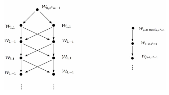
Figure 12: Structure of standard modules for $\mathfrak{q}=e^{i\pi/2}$.

Meanwhile, we can read the dimension content from the general formulae:

$$F_{j,1}={1\over(q\bar{q})^{-2/24}P(q)P(\bar{q})}\sum_{e\in\mathbb{Z}}q^{{(j-2e)^{2}-1\over 8}}\bar{q}^{{(j+2e)^{2}-1\over 8}}\,.$$ (226)

Let us consider in more detail $F_{1,1}$. This contains the exponents $(h,\bar{h})$, here ordered by the total value of the scaling dimension $h+\bar{h}$:

$$(0,0);(0,1)\times 2;(1,0)\times 2;(1,1)\times 3;(2,0)\times 3;(0,2)\times 3;\ldots\,.$$ (227)

We see that the first eigenvalue with $h-\bar{h}=1$ is $(h,\bar{h})=(1,0)$, the first eigenvalue with $h-\bar{h}=2$ is $(h,\bar{h})=(2,0)$, etc. This agrees with the expansion (215). Since only purely chiral contributions appear in this expansion, this means that, for a given value of $n=h-\bar{h}$, we have only the smallest realisation, $(h,\bar{h})=(n,0)$. The same applies to all the other sectors.

B.4.2 The four-point function $P_{abab}-P_{abba}$

We now go back to the combination $P_{abab}-P_{abba}$, which we write in terms of the variable $z\equiv{z_{12}z_{34}\over z_{13}z_{24}}$:

$$P_{abab}-P_{abba}\propto-[\ln(1-z)+\ln(1-\bar{z})]\,,$$ (228)

and expanding this we get

$$P_{abab}-P_{abba}\propto\sum_{n=1}^{\infty}{z^{n}+\bar{z}^{n}\over n}\,.$$ (229)

Note that, if we exchange points 1 and 2, we have $z={z_{12}z_{34}\over z_{13}z_{24}}\to{z_{21}z_{34}\over z_{23}z_{14}}={z\over z-1}$. This corresponds to sending $1-z\to{1\over 1-z}$, and thus to changing the sign of $P_{abab}-P_{abba}$, as required from the geometrical interpretation. This does not mean that only odd spins appear in the expression (28), because in this case there are large degeneracies (in fact, only a few of the terms correspond to primary fields).

Going to the cylinder as usual we find now

$$P_{abab}-P_{abba}\propto\sum_{n=1}^{\infty}{(-1)^{n}\over n}\left(4\sin^{2}{2\pi a\over L}\right)^{n}{\xi^{n}\over(1-\xi)^{2n}}+\hbox{ h.c.}$$ (230)

To compare with the numerical work, we rewrite (230) as

$$P_{abab}-P_{abba}\propto\sum_{n=1}^{\infty}C_{n}\xi^{n}+\hbox{ h.c.}$$ (231)

and choose the normalisation $C_{1}=1$, so that the amplitude ratios can be read off directly from the following coefficients. The first few then read explicitly

$$C_{2} = 2\left(\cos\frac{2\pi a}{L}\right)^{2}\,,$$ (232a)

$$C_{3} = \frac{1}{3}\left(1+2\cos\frac{4\pi a}{L}\right)^{2}\,,$$ (232b)

$$C_{4} = \left(\cos\frac{2\pi a}{L}+\cos\frac{6\pi a}{L}\right)^{2}\,.$$ (232c)

As above, the numerical work was done for $L=5$ and $2a=2$ (resp. $L=7$ and $2a=3$). The contributing eigenvalues are then found to be exactly the same as for the two-point function $g_{2}(1,2)$, corresponding to the terms $n=1,2$ (resp. $n=1,2,3$) in (231). There is no longer any Jordan cell (the term $n=0$). Note also that in both cases, we expect at all orders to have only chiral or antichiral contributions. The numerical results compared with the conformal predictions run as follows:

$$\begin{array}[]{ll|lll}L&&C_{2}/C_{1}&C_{3}/C_{1}\\ \hline\cr 5&{\rm lattice}&0.1984202998&-\\ &{\rm CFT}&0.1909830056&\\ &{\rm ratio}&1.0389&\\ \hline\cr 7&{\rm lattice}&0.09439172580&0.2233910496\\ &{\rm CFT}&0.09903113209&0.2143680440\\ &{\rm ratio}&0.9532&1.0421\\ \hline\cr\end{array}$$ (240)

Once again the agreement is very reasonable, given the rather small sizes.

A peculiarity of this four-point function—as well as of the two-point function $g_{2}$ considered above—is that only fields with $h=0$ or $\bar{h}=0$ appear. Since the spin $h-\bar{h}$ is limited to values $0,1,\ldots,L-1$ for a finite size $L$, this means only a very small number of eigenvalues contribute to the correlation function at finite $L$. This is quite different from the usual case, where having $h-\bar{h}$ fixed does not preclude eigenvalues with larger $h+\bar{h}$ from contributing. Of course, it could be that some eigenvalues would contribute in finite $L$, although their amplitude would tend to zero when $L$ increases, because they would not be present in the continuum limit. But this does not seem to be the case here—a fact that can probably be proven exactly in finite size using the Laplacian on the cylinder.

B.4.3 The combination $P_{aabb}-P_{abba}$

It is also interesting to observe that, under crossing $z_{2}\leftrightarrow z_{3}$, ie $z\to{1\over z}$, the combination $P_{abab}-P_{abba}$ that we have just discussed becomes $P_{aabb}-P_{abba}$. We have studied the latter combination independently. From our analytical result (228) we now find

$$P_{aabb}-P_{abba}\propto\ln z-\ln(1-z)+\ln\bar{z}-\ln(1-\bar{z})\,.$$ (241)

Hence on the cylinder we expect

$$P_{aabb}-P_{abba}\propto\ln(4\sin^{2}(2\pi a/L))+\ln\xi+\sum_{n=1}^{\infty}\left(2{\xi^{n}\over n}+{(-4\sin^{2}(2\pi a/L))^{n}\over n}{\xi^{n}\over(1-\xi)^{2n}}\right)+\hbox{h.c.}\,.$$ (242)

It is easy to ascertain that the correct sectors are observed in the numerical study. Indeed we observe now again a Jordan cell on the ground state, plus the same 2 (resp. 3) simple eigenvalues as before for the case $L=5$ and $2a=2$ (resp. $L=7$ and $2a=3$). The indecomposability parameter, i.e., the coefficient multiplying $l$ in the correlation function, is found to be $A=\frac{1}{L}$ exactly in finite size, like it was for the two-point function. Let us write the remaining terms, concerning the simple eigenvalues, as $\sum_{n=1}^{\infty}D_{n}\xi^{n}+\hbox{ h.c.}$ The comparison with numerics can then be summarised as follows:

$$\begin{array}[]{ll|lll}L&&D_{2}/D_{1}&D_{3}/D_{1}\\ \hline\cr 5&{\rm lattice}&-0.1984202998&-\\ &{\rm CFT}&-0.1909830056&\\ &{\rm ratio}&1.0389&\\ \hline\cr 7&{\rm lattice}&-0.3298008395&0.08579175620\\ &{\rm CFT}&-0.3460107358&0.08232653457\\ &{\rm ratio}&0.9532&1.0421\\ \hline\cr\end{array}$$ (250)

It will not have escaped the reader’s attention that the ratios are exactly the same as for the previously considered case $P_{abab}-P_{abba}$. This presumably extends to arbitrary $L$ and implies that the symmetry $z\to\frac{1}{z}$ is respected exactly on the lattice—something that we again suspect can be proven by a careful study of the Laplacian on the cylinder. Per se, this close relationship between the foregoing two four-point functions is pretty remarkable, since after all, in the lattice study of $P_{abab}$ we have two long clusters, while in $P_{aabb}$ we have two short ones.

References

- [1] M. Picco, S. Ribault and R. Santachiara, A conformal bootstrap approach to critical percolation in two dimensions, SciPost Phys. 1, 009 (2016); arXiv:1607.07224.
- [2] C.M. Fortuin and P.W. Kasteleyn, On the random-cluster model: I. Introduction and relation to other models, Physica 57, 536–564 (1972).
- [3] R.B. Potts, Some generalized order-disorder transformations, Math. Proc. Cambr. Phil. Soc. 48, 106–109 (1952).
- [4] P. Di Francesco, D. Sénéchal and P. Mathieu, Conformal field theory (Springer-Verlag, New York, 1997).
- [5] A.B. Zamolodchikov, Conformal symmetry in two dimensions: An explicit recurrence formula for the conformal partial wave amplitude, Comm. Math. Phys. 96, 419–422 (1984).
- [6] A.B. Zamolodchikov, Conformal symmetry in two-dimensional space: Recursion representation of conformal block, Theor. Math. Phys. 73, 1088-1093 (1987).
- [7] P. Di Francesco, H. Saleur and J.B. Zuber, Relations between the Coulomb gas picture and conformal invariance of two-dimensional critical models, J. Stat. Phys. 49, 57–79 (1987).
- [8] R.J. Baxter, Potts model at the critical temperature, J. Phys. C: Solid State Phys. 6, L445 (1973).
- [9] R.J. Baxter, S.B. Kelland and F.Y. Wu, Equivalence of the Potts model or Whitney polynomial with an ice-type model, J. Phys. A: Math. Gen. 9, 397 (1976).
- [10] H.N.V. Temperley and E.T. Lieb, Relation between the ‘percolation’ and ‘colouring’ problem and other graph-theoretical problems associated with planar lattices: some exact results for the ‘percolation’ problem, Proc. Roy. Soc. London A 322, 251 (1971).
- [11] R. Vasseur and J.L. Jacobsen, Critical properties of joint spin and Fortuin-Kasteleyn observables in the two-dimensional Potts model, J. Phys. A: Math. Theor. 45, 165001 (2012); arXiv:1111.4033.
- [12] J. Dubail, J.L. Jacobsen and H. Saleur, Critical exponents of domain walls in the two-dimensional Potts model, J. Phys. A: Math. Theor. 43, 482002 (2010); arXiv:1008.1216.
- [13] J. Dubail, J.L. Jacobsen and H. Saleur, Bulk and boundary critical behaviour of thin and thick domain walls in the two-dimensional Potts model, J. Stat. Mech. (2010) P12026; arXiv:1010.1700.
- [14] G. Delfino and J. Viti, Potts -color field theory and scaling random cluster model, Nucl. Phys. B 852, 149–173 (2011); arXiv:1104.4323.
- [15] B. Nienhuis, Critical behavior of two-dimensional spin models and charge asymmetry in the Coulomb gas, J. Stat. Phys. 34, 731 (1984).
- [16] B. Duplantier and H. Saleur, Exact critical properties of two-dimensional dense self-avoiding walks, Nucl. Phys. B. 290, 291–326 (1987).
- [17] M. Picco, R. Santachiara, J. Viti and G. Delfino, Connectivities of Potts Fortuin-Kasteleyn clusters and time-like Liouville correlator, Nucl. Phys. B 875, 719–737 (2013); arXiv:1304.6511.
- [18] Y. Ikhlef, J.L. Jacobsen and H. Saleur, Three-point functions in Liouville theory and conformal loop ensembles, Phys. Rev. Lett. 116, 130601 (2016); arXiv:1509.03538.
- [19] R. Vasseur, J.L. Jacobsen and H. Saleur, Logarithmic observables in critical percolation, J. Stat. Mech. L07001 (2012); arXiv:1206.2312.
- [20] R. Vasseur and J.L. Jacobsen, Operator content of the critical Potts model in d dimensions and logarithmic correlations, Nucl. Phys. B 880, 435–475 (2014); arXiv:1311.6143.
- [21] R. Couvreur, J.L. Jacobsen and R. Vasseur, Non-scalar operators for the Potts model in arbitrary dimension, J. Phys. A: Math. Theor. 50, 474001 (2017); arXiv:1704.02186.
- [22] T. Halverson and A. Ram, Partition algebras, Eur. J. Combin. 26, 869–921 (2005).
- [23] R.J. Baxter, Exactly Solved models in statistical mechanics (Academic Press, London, 1982).
- [24] P.P., Martin, Potts models and related problems in statistical mechanics (World Scientific, Singapore, 1991).
- [25] P.P. Martin and H. Saleur, The blob algebra and the periodic Temperley-Lieb algebra, Lett. Math. Phys. 30, 189–206 (1994).
- [26] J.J. Graham and G.I. Lehrer, The representation theory of affine Temperley-Lieb algebras, L’Ens. Math. 44, 173 (1998).
- [27] A.M. Gainutdinov, N. Read, H. Saleur and R. Vasseur, The periodic alternating spin chain and its continuum limit as a bulk LCFT at , JHEP (2015) 114.
- [28] A.M. Gainutdinov, J.L. Jacobsen and H. Saleur, A fusion for the periodic Temperley-Lieb algebra and its continuum limit, arXiv:1712.07076.
- [29] V.F.R. Jones, Quotient of the affine Hecke algebra in the Brauer algebra, L’Ens. Math. 40, 313 (1994).
- [30] N. Read and H. Saleur, Enlarged symmetry algebras of spin chains, loop models, and -matrices, Nucl. Phys. B 777, 263–315 (2007); arXiv:cond-mat/0701259.
- [31] J.-F. Richard and J.L. Jacobsen, Eigenvalue amplitudes of the Potts model on a torus, Nucl. Phys. B 769, 256–274 (2007); arXiv:math-ph/0608055.
- [32] J.L. Jacobsen and J. Salas, Phase diagram of the chromatic polynomial on a torus, Nucl. Phys. B 783, 238–296 (2007); arXiv:cond-mat/0703228.
- [33] J.L. Jacobsen and P. Zinn-Justin, A transfer matrix for the backbone exponent of two-dimensional percolation, J. Phys. A: Math. Gen. 35, 2131 (2002); arXiv:cond-mat/0111374.
- [34] J.L. Jacobsen and P. Zinn-Justin, Monochromatic path crossing exponents and graph connectivity in two-dimensional percolation, Phys. Rev. E 66, 055102(R) (2002); arXiv:cond-mat/0207063.
- [35] Y. Deng, H.W.J. Blöte and B. Nienhuis, Backbone exponents of the two-dimensional -state Potts model: A Monte Carlo investigation, Phys. Rev. E 69, 026114 (2004).
- [36] Z. Zhou, J. Yang, Y. Deng and R.M. Ziff, Shortest-path fractal dimension for percolation in two and three dimensions, Phys. Rev. E 86, 061101 (2012); arXiv:1112.3428.
- [37] A.M. Gainutdinov, N. Read and H. Saleur, Continuum limit and symmetries of the periodic spin chain, Nucl. Phys. B 871, 245–288 (2013); arXiv:1112.3403.
- [38] A.M. Gainutdinov, N. Read and H. Saleur, Bimodule structure in the periodic spin chain, Nucl. Phys. B 871, 289–329 (2013); arXiv:1112.3407.
- [39] A.M. Gainutdinov, N. Read and H. Saleur, Associative algebraic approach to logarithmic CFT in the bulk: the continuum limit of the periodic spin chain, Howe duality and the interchiral algebra, Comm. Math. Phys. 341, 35–103 (2016); arXiv:1207.6334.
- [40] A.M. Gainutdinov, J.L. Jacobsen, H. Saleur and R. Vasseur, A physical approach to the classification of indecomposable Virasoro representations from the blob algebra, Nuclear Physics B 873 (3), 614–681 (2013); arXiv:1212.0093.
- [41] A.M. Gainutdinov, J.L. Jacobsen, N. Read, H. Saleur and R. Vasseur, Logarithmic conformal field theory: a lattice approach, J. Phys. A: Math. Theor. 46, 494012 (2013); arXiv:1303.2082.
- [42] J. Belletête, A.M. Gainutdinov, J.L. Jacobsen, H. Saleur and R. Vasseur, On the correspondence between boundary and bulk lattice models and (logarithmic) conformal field theories, J. Phys. A: Math. Theor. 50, 484002 (2017); arXiv:1705.07769.
- [43] A. Belavin, A. Polyakov and A.B. Zamolodchikov, Infinite conformal symmetry in two-dimensional quantum field theory, Nucl. Phys. B 241, 333–380 (1984).
- [44] V. Pasquier and H. Saleur, Common structures between finite systems and conformal field theories through quantum groups, Nucl. Phys. B 330, 523–556 (1990).
- [45] F.C. Alcaraz, U. Grimm and V. Rittenberg, The XXZ Heisenberg chain, conformal invariance and the operator content of systems, Nucl. Phys. B 316, 735 (1989).
- [46] M.P.M. den Nijs, Extended scaling relations for the magnetic critical exponents of the Potts model, Phys. Rev. B 27, 1674 (1983).
- [47] J.L. Jacobsen and H. Saleur, Combinatorial aspects of boundary loop models, J. Stat. Mech. (2008) P01021; arXiv:0709.0812.
- [48] J. de Gier, J.L. Jacobsen and A. Ponsaing, Finite-size corrections for universal boundary entropy in bond percolation, SciPost Phys. 1, 012 (2016); arXiv:1610.04006.
- [49] B. Estienne and Y. Ikhlef, Correlation functions in loop models; arXiv:1505.00585.
- [50] S. Migliaccio and S. Ribault, The analytic bootstrap equations of non-diagonal two-dimensional CFT; arXiv:1711.08916.
- [51] I. Runkel and G.M.T. Watts, A non-rational CFT with as a limit of minimal models, JHEP 0109 (2001) 006; arXiv:hep-th/0107118.
- [52] S. Ribault and R. Santachiara, Liouville theory with central charge less than one, JHEP (2015) 2015: 109.
- [53] W.M. Koo and H. Saleur, Representations of the Virasoro algebra from lattice models, Nucl. Phys. B 426, 459–504 (1994).
- [54] J.L. Jacobsen, S. Ribault, H. Saleur and Linnéa Gräns Samuelsson, in preparation.
- [55] H.W.J. Blöte and M.P. Nightingale, Critical behaviour of the two-dimensional Potts model with a continuous number of states: A finite size scaling analysis, Physica A 112, 405–465 (1982).
- [56] J. Salas and A.D. Sokal, Transfer matrices and partition-function zeros for antiferromagnetic Potts models. I. General theory and square-lattice chromatic polynomial, J. Stat. Phys. 104, 609–699 (2001); arXiv:cond-mat/0004330.
- [57] S.C. Chang, J. Salas and R. Shrock, Exact Potts model partition functions for strips of the square lattice, J. Stat. Phys. 107, 1207–1253 (2002); cond-mat/0108144.
- [58] F.M. Gomes and D.C. Sorensen, Arpack++. An object-oriented version of ARPACK eigenvalue package, https://www.caam.rice.edu//software/ARPACK/arpack++.html.
- [59] B. Haible and R.B. Kreckel, CLN – Class library for numbers, https://www.ginac.de/CLN.
- [60] J.L. Jacobsen, Critical points of Potts and O() models from eigenvalue identities in periodic Temperley-Lieb algebras, J. Phys. A: Math. Theor. 48, 454003 (2015); arXiv:1507:03027.
- [61] J.L. Jacobsen, C.R. Scullard and A.J. Guttmann, On the growth constant for square-lattice self-avoiding walks, J. Phys. A: Math. Theor. 49, 494004 (2016); arXiv:1607:02984.
- [62] J.L. Jacobsen, J. Salas and C.R. Scullard, Phase diagram of the triangular-lattice Potts antiferromagnet, J. Phys. A: Math. Theor. 50, 345002 (2017); arXiv:1702:02006.
- [63] B. Mc Coy and T.T. Wu, The two-dimensional Ising model (Harvard University Press, 1973).
- [64] A. Rocha-Caridi, in Vertex operators in mathematics and physics, MSRI Publications 3, 451–473 (Springer-Verlag, Heidelberg, 1984).
- [65] P. Reinicke and T. Vescan, Finite-size corrections to matrix elements in a conformal theory. Applications to the magnetisation of the three-state Potts model, J. Phys. A: Math. Gen. 20, L653 (1987).
- [66] S.K. Yang, Modular invariant partition function of the Ashkin-Teller model on the critical line and superconformal invariance, Nucl. Phys. B 285, 183–203 (1987).
- [67] Al. B. Zamolodchikov, Two-dimensional conformal symmetry and critical four-spin correlation functions in the Ashkin-Teller model, Sov. Phys. JETP 63, 1061 (1986).
- [68] J.L. Jacobsen, J. Salas and A.D. Sokal, Spanning forests and the -state Potts model in the limit , J. Stat. Phys. 119, 1153–1281 (2005); arXiv:cond-mat/0401026.
- [69] S. Caracciolo, J.L. Jacobsen, H. Saleur, A.D. Sokal and A. Sportiello, Fermionic field theory for trees and forests, Phys. Rev. Lett. 93, 080601 (2004); arXiv:cond-mat/0403271.
- [70] J.L. Jacobsen and H. Saleur, The arboreal gas and the supersphere sigma model, Nucl. Phys. B 716, 439–461 (2005); arXiv:cond-mat/0502052.
- [71] H. Saleur, Polymers and percolation in two dimensions and twisted supersymmetry, Nucl. Phys. B 382, 486–531 (1992).
- [72] E.V. Ivashkevich, Correlation functions of dense polymers and conformal field theory, J. Phys. A: Math. Gen. 32, 1691 (1999).
- [73] G. Kirchhoff, Ueber die Auflösung der Gleichungen, auf welche man bei der Untersuchung der linearen Vertheilung galvanischer Ströme geführt wird, Ann. Phys. Chem. 72, 497–508 (1847).
- [74] V.B. Priezzhev, The dimer problem and the Kirchhoff theorem, Sov. Phys. Usp. 28, 1125 (1985).
- [75] H.G. Kausch, Curiosities at , arXiv:hep-th/9510149.
- [76] H.G. Kausch, Symplectic fermions, Nucl. Phys. B 583, 513–541 (2000).
- [77] J.M. Luck, Finite-size scaling and the two-dimensional XY model, J. Phys. A: Math. Gen. 15, L169 (1982).