New Insights into Time Series Analysis III
Setting constraints on period analysis

Abstract

E-science of photometric data requires automatic procedures and a precise recognition of periodic patterns to perform science as well as possible on large data. Analytical equations that enable us to set the best constraints to properly reduce processing time and hence optimize signal searches play a crucial role in this matter. These are increasingly important because the production of unbiased samples from variability indices and statistical parameters has not been achievable so far. We discuss the constraints used in periodic signals detection methods as well as the uncertainties in the estimation of periods and amplitudes. The frequency resolution necessary to investigate a time series is assessed with a new approach that estimates the necessary sampling resolution from shifts on the phase diagrams for successive frequency grid points.We demonstrate the underlying meaning of the oversampling factor. We reassess the frequency resolutions required to find the variability periods of $EA$ stars and use the new resolutions to analyse a small sample of $EA_{up}$ Catalina stars, i.e. $EA$ stars previously classified as having insufficient number of observations at the eclipses. As a result, the variability periods of four $EA_{up}$ stars were determined. Moreover, we have a new approach to estimate the amplitude and period variations. From these estimations information about the intrinsic variations of the sources are obtained. For a complete characterization of the light curve signal the period uncertainty and period variation must be determined. Constraints on periodic signal searches were analysed and delimited.

1 Introduction

Some time series are stochastic (or random) in the sense that they do not contain underlying information other than noise. The analysis of large databases requires automatic and efficient classifiers to provide the identification of genuine features. This is crucial to reduce the number of misclassifications, to narrow the boundaries between classes, to provide better training sets, as well as to diminish the total processing time (Eyer, 2006). Large volumes of data containing potentially interesting scientific results are left unexplored or have their analysis delayed due to the current limited inventory of tools which are unable to produce clean samples, despite big efforts having been undertaken. In fact, we risk underusing a large part of these data. In order to improve the efficiency of variability indices, we propose discriminating variable sources in correlated and non-correlated data. The correlated data have several measurements close in time, from which accurate correlated indices are computed. On the other hand, the non correlated data are those sources having too few measurements close in time and so they must be analysed using statistical parameters only. The use of correlated and non-correlated indices (see Sect. 4.3 in Ferreira Lopes & Cross, 2016), produces a substantially smaller number of time series which have to be further analysed. However, the resulting selection is still three or more times larger than just the well-defined signals, according to Ferreira Lopes & Cross (2016, 2017). This means that the set of preliminary selection criteria is unable to produce samples comprised only of variable stars, and so, it would be desirable that the following steps of signal searching methods would provide reliable identifications and accurate estimates of periods (frequencies) and amplitudes, even in cases where the preliminary analysis failed to give a confident indicator that the signal was truly variable and not just a noisy time series. Indeed, $\sim 75\%$ of parameters used to characterize light curves are derived from the folded light curve using the variability periods (Richards et al., 2011). This led to a $\sim 11\%$ misclassification rate for non-eclipsing variable stars, for instance, Dubath et al. (2011). Nowadays, reliable samples, i.e. samples composed only of variable stars, are increasingly becoming more important than complete samples, i.e samples having all variable stars but also having a large number of misclassified non-variable stars, since visual inspection of all sources is unfeasible. Therefore, an approach that allows us to get unbiased samples having correct periods is mandatory to return quicker scientific results. Therefore, as a continuation of the “New Insights into Time Series Analysis” project, the frequency finding methods are reviewed and improved.

The periodic signals finding methods can be separated into three main groups if we consider how each component of the figure of merit in the frequency grid is computed: $M_{S}$ - each epoch provides a single term; $M_{P}$ - each term is computed using a pair of epochs; $M_{B}$ - each term is computed by binning the phase diagram. The Lomb Scargle and its generalization (LS - Lomb 1976; Scargle 1982 and GLS - Zechmeister & Kürster 2009) belong to the $M_{S}$ group. Each epoch is regarded as a single power spectrum term and the periodogram is equivalent to a least squares fit of the folded data at each frequency by a sine wave. Indeed, Fourier methods and their branches are the simplest methods belong to the $M_{S}$ group. On the other hand, the string length method (STR - Dworetsky, 1983) and the analysis of variance (AOV and AOVMHW - Schwarzenberg-Czerny, 1989, 1996) belong to the $M_{P}$ group. However, they follow different approaches since the STR power spectrum is computed using pairs of epochs in the phase diagram while AOV pairs epochs in time. Phase dispersion minimization (PDM and PDM2 - Stellingwerf, 1978, 2011), conditional entropy (CE - Graham et al., 2013), supersmoother (SS - Reimann, 1994), and correntropy kernel periodogram (CKP - Huijse et al., 2012) belong to the $M_{B}$ group, where the power spectrum is computed by binning the phase diagram. Wavelet analysis also has been used to study time series (e.g. Foster, 1996; Bravo et al., 2014). However it is more suitable to study the evolution of a signal over time and it requires continuous observation. Currently, these are the main frequency finding methods but there are many others (e.g. Huijse et al., 2011; Kato & Uemura, 2012).

The efficiency of the frequency finding methods has been tested in the last few years (e.g. Heck et al., 1985; Swingler, 1989; Schwarzenberg et al., 1999; Distefano et al., 2012; Graham et al., 2013). Usually, the authors analyze the sensitivity as well as the fraction of true periods recovered within a defined accuracy limit. Indeed, research using real data, including for instance irregular sampling, gaps, outliers, and errors, may provide more reliable results. Currently, the most complete of these studies was performed by Graham et al. (2013). The authors analysed 11 different methods using light curves of $78$ variable star types. The conditional entropy-based algorithm is the most optimal in terms of completeness and speed according to the authors. However, most frequency finding methods have a selection effect for the identification of weak periodic signals de Jager et al. (1989); Schwarzenberg-Czerny (1999). Therefore a combination of all methods could potentially increase the recover rate close to $100\%$ according to Dubath et al. (2011). However, which method leads to the correct period for a specific light curve within an automated strategy is an open question. Moreover, the main frequencies computed by different methods can be dissimilar and so two questions must be answered to determine the best way to analyse a time series, i.e. how many frequency finding methods should be combined and how to work out which period should be chosen when two or more methods provide different results?

The frequency finding methods adopt, as the true frequency ($\mathrm{f_{true}}$), one that defines the main periodic variation displayed by the time series, based on a minimum or maximum of the quantity being tested. However, the main frequency can be a harmonic of $\mathrm{f_{true}}$ or related to an instrumental or spurious variation. It means that only using the period finding method is not enough to set a reliable period and so additional analyses are required. For example, the harmonic fits can be used to set models and, using the $\chi^{2}$ distribution, establish $\mathrm{f_{true}}$ and its reliability (Ferreira Lopes et al., 2015a). However, what $\chi^{2}$ threshold, below which a time series may be considered to have a reliable signal, and if the $\chi^{2}$ alone is enough to do that are open questions. Theoretically, any signal having an amplitude greater than the noise could be detected using a suitable method. The false alarm probability (FAP) has been used to determine the typical power spectrum values of the noise and to discard variability due to noise alone. However, sources lacking a periodic signal, such as aperiodic variations and pulses, will also be discarded using this approach. All the period finding methods that depend on the phase diagram are unfit to detect these signals because no frequency will return a smooth phase diagram. Therefore, classifying a time series as noisy requires an investigation of all signal types. On the other hand, correlated noise, seasonal variations, the cadence or the phase coverage can lead to power values above the FAP indicating an applicability limit to using this approach to determine the reliability of selections. Indeed, a large number of Monte-Carlo simulations are usually performed to determine the FAP and hence the running time required should also be taken into account. Then our required list of improvements towards an efficient automation of the variability analysis should include: how to use the current period finding methods to determine the reliability of signals? How to discriminate aperiodic from stochastic variations? Is it possible to study all variation types using a single approach or are different strategies required for different purposes? How to provide a standard cutoff to determine reliable signals?

Currently, any frequency finding method is able to compute $\mathrm{f_{true}}$ using a single computation. Therefore, the determination of $\mathrm{f_{true}}$ is performed after computing several times a function that is susceptible to the smoothness of the phase diagrams depending on the method that is used. The phase values are given by;

$$\mathrm{\phi_{i}=t_{i}\times f_{test}-{\rm\mathrm{\textit{G}}}\left[t_{i}\times\mathrm{f_{test}}\right]},$$ (1)

where $t_{i}$ is the time, $\mathrm{f_{test}}$ is a test frequency, and the function G returns the integer part of $t_{i}\times\mathrm{f_{test}}$. This equation provides an interval of values ranging $0\leq\Phi\leq 1$ where $\mathrm{f_{true}}$ is the frequency which returns the smoothest phase diagram. The minimum ($\mathrm{f_{min}}$) and maximum ($\mathrm{f_{max}}$) frequency as well as the resolution ($\Delta\mathrm{f}$) or number of frequencies ($\mathrm{N_{f}}$) are required as inputs to search periods in all unevenly spaced time series for all frequency finding methods. The $\mathrm{f_{min}}$ is usually defined as $2/T_{tot}$, where $T_{tot}$ is the total timespan of the observations. This definition is commonly used as a requirement to enclose at least two variability cycles in the time series. However, variations having fewer than two cycles can be considered with caution when biases have been identified and removed (e.g. De Medeiros et al., 2013; Ferreira Lopes et al., 2015b). On the other hand, $\mathrm{f_{max}}$ will be linked with the time interval between the observations $\delta t$. The Nyquist frequency ($\mathrm{f_{max}}=0.5/\delta t$) must be assumed for evenly-spaced time series since this constitutes an upper limit to the frequency range over which a periodogram can be uniquely calculated. Otherwise, for irregularly sampled cases, the frequency limit becomes dominated by the exposure time (Eyer & Bartholdi, 1999).

The frequency sampling strategy is crucial to determine $\mathrm{f_{true}}$ using any frequency finding algorithm. A small variation on $\mathrm{f_{true}}$ provides a big variation in the phase diagram mainly when $f_{true}\times\,T_{tot}>>1$ (see Sect. 2). It means that $\mathrm{f_{true}}$ can be missed if the periodogram is not computed for a sufficiently large number of test frequencies. A reasonable criterion (see previous paragraph) has been used to determine $\mathrm{f_{min}}$ while an empirical criterion has been applied to set $\mathrm{f_{max}}$ and $\Delta\mathrm{f}$. For instance, $\mathrm{f_{min}}=0$, $\mathrm{f_{max}}=10d^{-1}$, and $\Delta\mathrm{f}=0.1/T_{tot}$ were adopted by Debosscher et al. (2007) and Richards et al. (2012). In this case, the authors assumed an empirical cutoff on the maximum frequency below which any reliable frequency could be found: the frequency finding method is able detect all reliable frequencies in a range of $\mathrm{f}\pm\Delta\mathrm{f}/2$. On the other hand, Schwarzenberg-Czerny (1996) assumes $\mathrm{f_{min}}=0$, $\mathrm{f_{max}}=1/2\tau_{med}$, and an optimal grid $\Delta\mathrm{f}=1/(A\times T_{tot})$, where $\tau_{med}$ is the median difference between successively ordered observation times and $A$ is a factor, typically ranging $10-15$, which takes into account oversampling and binning or the number of harmonics used in the Fourier fit. Graham et al. (2013) tested $\Delta\mathrm{f}$ values of $0.0001$, $0.001$, $0.01$, and the optimal grid over a frequency range from $\mathrm{f_{min}}=0$ to $\mathrm{f_{max}}=20$ for standard frequency finding methods; LS, GLS, AOVs, PDMs, STR, FC, CE, SS, and CKP methods. The data test used by the authors has a number of observations ranging from $105$ to $966$ and a total baseline ranging from $2182$ to $2721$ days. The performance found for $\Delta\mathrm{f}=0.0001$ and the optimal $\Delta\mathrm{f}$ (the median optimal $\Delta\mathrm{f}$ is $2.5\times 10^{-5}$) is quite similar for all methods analysed according to the authors. Indeed these results can only be used as a guide for samples that mimic those tested by the authors since the samples tested do not cover all possible intervals of measurements and baselines. Therefore, what is the optimal resolution able to detect all periodic variations and how much finer grain is necessary to get a more accurate period estimation, if $\mathrm{f_{true}}$ is found since an initial value can be found with a coarser grain resolution, are open questions.

The majority of frequency finding methods were designed for single time series. Such methods are in accordance with past surveys since they were usually from observations in a single photometric waveband (e.g. VVV - Minniti et al. 2010, LINEAR - Sesar et al. 2011, CoRoT - Baglin et al. 2007, and Kepler - Borucki et al. 2010). However, in the last few years there are multi-wavelength surveys like Gaia (Bailer-Jones et al., 2013), where the main catalogue is multi-epoch using a wide G filter, but it also contains colour information from simultaneous multi-epoch low resolution spectra. Period finding could be done on G-band and forthcoming surveys like LSST (Ivezic et al., 2008) require multi-wavelength frequency finding methods in order to optimize the period searches. Usually each waveband is analysed separately and posteriorly the results are combined (e.g. Oluseyi et al., 2012; Ferreira Lopes et al., 2015a). However, the combination of different datasets allows us to increase the number of measurements that are extremely important to signal detection. Süveges et al. (2012) used principal component analysis to extract the best period from analysis of the Welch-Stetson variability index (Welch & Stetson, 1993). However, the method requires observations taken simultaneously. VanderPlas & Ivezić (2015) introduce a multi-band periodogram by extending the Lomb-Scargle approach. For that, the authors modeled each waveband as an arbitrary truncated Fourier series using the Tikhonov regularization in order to provide a common model at all wavebands. Such methods and new insights into multi-wavelength frequency finding methods are required to take full advantage of the multi-wavelengths observations.

The discussion above provokes questions that must be addressed in the challenge to analyze large amount of photometric data automatically. Some of these questions are addressed in the current paper (III) and the forthcoming papers of this series will address the remaining questions. Sections 2 and 3 assess the frequency sampling and frequency uncertainties. Sect. 4 establishes an approach to compute period and amplitude variations. In Sect. 5 we show our results on estimating frequency resolution and uncertainties, and discuss them. We address our final remarks in Sect. 6.

2 Frequency sampling

Consider a periodic signal modeled by function $\mathrm{F}$ having frequency $\mathrm{f_{true}}$ (being a real, positive constant) where $\mathrm{F=\left[F(\,t_{1}\,),F(\,t_{2}\,),\cdots,F(\,t_{n}\,)\right]}$. From which $\mathrm{F(\,t_{i}\,)=F(\,t_{i}+n_{c}/\mathrm{f_{true}}\,)}$ where $n_{c}$ (number of cycles) is a positive integer ranging from zero to $G[T_{tot}\times f_{true}]$. This relationship is also true for phase values, i.e. $\mathrm{\phi_{i}(\,t_{i}\,)=\phi(\,t_{i}+n_{c}/\mathrm{f_{true}}\,)=\phi_{j}(\,t_{j}\,)}$ and therefore $\left|\mathrm{\phi_{j}\,-\,\phi_{i}}\right|=0$. The phase difference between them for a frequency given by $\mathrm{f=f_{true}+\delta f}$ is written as,

$$\scriptsize\left|\mathrm{\phi_{j}\,-\,\phi_{i}}\right| = \Bigl{|}\mathrm{t_{j}\times\left(f_{true}+\delta f\right)-G\bigl{[}t_{j}\times\left(f_{true}+\delta f\right)\bigr{]}}$$

$$\mathrm{-t_{i}\times\left(f_{true}+\delta f\right)+G\left[t_{i}\times\left(f_{true}+\delta f\right)\right]}\Bigr{|}$$

$$\left|\mathrm{\phi_{j}\,-\,\phi_{i}}\right| = \Bigl{|}\mathrm{\left(t_{j}-t_{i}\right)\times\delta f+\Bigl{\{}t_{j}\times f_{true}-G\left[t_{j}\times\left(f_{true}+\delta f\right)\right]\Bigr{\}}}$$ (2)

$$\mathrm{-\Bigl{\{}t_{i}\times f_{true}-G\left[t_{i}\times\left(f_{true}+\delta f\right)\right]\Bigr{\}}\Bigr{|}}.$$

Having $\mathrm{\delta f<<f}$ implies that $\mathrm{G\left[t\times\left(f+\delta f\right)\right]=G\left[t\times f\right]}$. Indeed, this is reasonable since the frequency sampling is usually set as $\mathrm{f_{n}=f_{min}+n\times\delta f}$. For instance, $n=100$ implies that there is a frequency at least hundred times greater than $\mathrm{\delta f}$. Considering this limit, the two last terms (in curly brackets) of Eq. 2 are cancelled and so,

$$\mathrm{\bigr{|}\phi_{j}\,-\,\phi_{i}\bigr{|}\simeq\bigr{|}t_{j}-t_{i}\bigr{|}\times\delta f}\implies\mathrm{\delta f\simeq\frac{\delta_{\phi_{j,i}}}{\bigr{|}t_{j}-t_{i}\bigr{|}}}$$ (3)

The maximum variation on $\mathrm{\delta_{\phi}}$ is found for $\left|t_{j}-t_{i}\right|=T_{tot}$, i.e. from the comparison among the measurements at the ends of the time series. Indeed, Eq. 3 was found only assuming that $\mathrm{\delta f<<f}$ and hence this expression can be used as an analytical definition of the frequency rate limit, where the number of frequencies is given by:

$$N_{f} = \frac{f_{max}-f_{min}}{\delta f}=\frac{\left(f_{max}-f_{min}\right)\times T_{tot}}{\delta_{\phi}}$$

$$N_{f} \simeq \frac{f_{max}\times T_{tot}}{\delta_{\phi}},$$ (4)

where $\mathrm{f_{max}>>f_{min}}$ was assumed when deriving the expression. This expression enables us to determine $N_{f}$ from the phase shift $\delta_{\phi}$ since $T_{tot}$ is a feature of a time series. On the other hand, $\mathrm{f_{max}}$ can be assumed to be the same for different time series, in the same set of observations, since the upper limit of frequencies, for those time series having evenly spaced data, is given by the Nyquist frequency (e.g. Eyer & Bartholdi, 1999). Therefore, the frequency search will be performed with the same resolution in the phase diagram if we assume the same $\delta_{\phi}$ for different time series. Moreover, it facilitates a strict comparison of frequency finding searches performed by different surveys.

Equation 4 was defined only by considering the phase diagram. Therefore, this relation is general and it can be used as an accurate determination of the frequency grid required to find any signal. Indeed, a similar equation has been used to estimate the frequency grid (e.g. Schwarzenberg-Czerny, 1996; Debosscher et al., 2007; Richards et al., 2012; VanderPlas & Ivezić, 2015; VanderPlas, 2018) where the $1/\delta_{\phi}$ is called the oversampling factor. However, no meaning had been provided for the oversampling factor so far. Values ranging from 5 to 15 have being adopted empirically only to ensure that the frequency grid is sufficient to sample each periodogram peak. The proper meaning of the oversampling factor is defined in Eq. 4 from which a suitable frequency grid for any kind of signal can be determined.

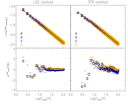
Figure 1: The logarithmic of FWHM as a function of logarithmic of $T_{tot}/P$ for the Generalized Lomb-Scargle (LSG - upper left panel) and for the string length (STR upper right panel) methods using four (ABCD) sinusoidal signal having models of variation and noise, shown in Fig 2 and described in Sect. 4. The models are set by colors and the solid black line marks the linear fits for LSG and STR methods. The percent relative errors ($\eta$) for both results are shown in the lower panels.

3 Frequency uncertainties

Frequency uncertainties were analytically defined from Fourier analysis (e.g. Kovacs, 1981; Gregory, 2001; Stecchini et al., 2017),

$$\sigma_{f}\propto\frac{1}{T_{tot}}\sqrt{\frac{1}{n\times\Sigma}}$$ (5)

where $n$ is the number of measurements, $\Sigma$ is the signal-to-noise ratio, and $T_{tot}$ is the total baseline of the observations. The uncertainty provided by a well defined periodic signal will be limited by the exposure time and hence Eq. 5 is not a suitable definition since it assumes an infinite accuracy. On the other hand, phenomena which result in small variations on the period can be mistaken for an increased uncertainty. Indeed, the uncertainties computed using a time series are given by the sum of intrinsic plus instrumental limitations. The uncertainties related with instrumental limitations can be estimated using a noise model (e.g. Ferreira Lopes & Cross, 2017) and by including this we can thus estimate the intrinsic variation. Some inconsistencies are found when the frequency uncertainty ($\sigma_{f}$ - see Eq. 5) estimation is related with $T_{tot}$, $n$, and $\Sigma$. For instance, a signal having an intrinsic variation in the frequency ($\sigma_{f}\neq 0$), such as light curves of rotational variables, may return a similar estimation of the uncertainty for time series having one hundred or one thousand measurements. On the other hand, for periodic signals a reduction in the dispersion about the model naturally occurs for a longer baseline and its accuracy is limited by instrumental properties instead for large $T_{tot}$ or $\Sigma$. Indeed, the power spectrum of $\mathrm{f_{true}}$ tends to a delta function with increasing $T_{tot}$ while increasing $n$ and $\Sigma$ improves the signal reliability since the probability of a signal being detected increases when the noise is reduced. These properties characterize the signal but they are not directly related with the period variations.

The CoRoT and Kepler databases have in common a large number of measurements and wide coverage time that provide unreliable uncertainty estimations using Eq. 5. Therefore, new approaches have been used to compute frequency uncertainties for semi-periodic signals. For the Kepler time series, Reinhold et al. (2013) compute the frequency uncertainty by fitting a parabola to the peak of the Lomb-Scargle power spectrum (Reinhold, private communication). On the other hand, for the CoRoT time series, De Medeiros et al. (2013) used a similar equation to that proposed by Lamm et al. (2004) to estimate the period uncertainty, given by

$$\delta P=\frac{\delta\nu\times P^{2}}{2},$$

where $\delta\nu$ is about $1/T_{tot}$ for non-uniform sampling according to the authors. Ferreira Lopes et al. (2015b, c) also used the CoRoT time series to study non-radial pulsation and stellar activity where the period uncertainties were estimated as the FWHM ($\delta P_{(\rm FWHM)}^{(\rm STR)}$) of the String Length power spectrum (Dworetsky, 1983). In particular, the amplitudes and periods vary for light curves of rotational variables that have differential rotation and spot evolution (e.g. Lanza et al., 2014; Reinhold & Gizon, 2015; Das Chagas et al., 2016). The analytical expression given by Eq. 5 or the analysis of the power spectrum are half-way to computing period variations in order to get new clues about physical phenomena that account for such variations.

Figure 1 shows $\delta P_{(\rm FWHM)}$ as a function of the number of cycles ($N_{(cycles)}=T_{tot}/P$) for the Generalized Lomb-Scargle (LSG- Zechmeister & Kürster, 2009) and for the string length (STR - Dworetsky, 1983) methods using the sinusoidal signal described in Sect. 4. The best fit models found for the LSG and STR methods are given by,

$$Log\left(\delta P_{(\rm FWHM)}^{(\rm LSG)}\right)=-1.00-0.44\times Log\left(\frac{T_{tot}}{P}\right)$$ (6)

and

$$Log\left(\delta P_{(\rm FWHM)}^{(\rm STR)}\right)=-0.97-0.54\times Log\left(\frac{T_{tot}}{P}\right).$$ (7)

We create 4 different sinusoidal models which are a single sinusoid (A), sinusoid plus amplitude variation (B), sinusoid plus period variation (C), and a sinusoid plus amplitude and period variations (D), see Sect. 4 and Fig. 2 for more details. However, the results are quite similar for all ABCD models, i.e. the $\delta P_{(\rm FWHM)}$ estimation is mainly defined by the $N_{(cycles)}$ instead of the time series properties. Indeed, it is highlighted for $N_{(cycles)}>10$ where the percent relative error (i.e. $\eta=100\times(theoretical-experimental)/\mid theoretical\mid$) is always smaller than $4\%$, see lower panels of Fig. 1. Eq. 6 is slightly different from Eq. 7 (see the solid lines in the two upper panels of Fig. 1) but the LSG method shows smaller relative errors ($\eta$). The approach using the FWHM of the power spectrum and any frequency finding method does not provide a trustworthy estimation of the period variation (for more detail see Sect. 5.4).

To summarise, the uncertainty computed using the power spectrum gives us a period interval about the variability period that leads to similar phase diagrams. Indeed, the main period and its uncertainty can vary for different period finding methods since the susceptibility to measuring phase diagram variations is not the same (e.g. Eyer, 2006; Graham et al., 2013). Moreover, the main period is assumed to be one that leads to the highest peak of periodogram that, a priori, gives the smoothest phase diagram and also the smallest residuals ($\sigma_{r}$), i.e. the standard deviation of observed data minus model (or predicted value). However, these assumptions have not been analysed so far, but this empirical criteria has been used all the time. In the sections below these questions are addressed.

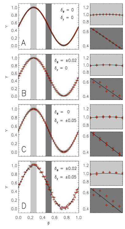
Figure 2: Sinusoidal light curves, with a fixed period and amplitude (A); with a varying period ($\delta_{\phi}=0.02$) and constant amplitude (B); varying amplitude ($\delta_{y}=0.05$) and constant period (C); and both amplitude and period variations (D). The black line shows the model while the red crosses show the measurements. The dark and light grey regions are expanded in the right panels.

4 Frequency and Amplitude Variations

Eq. 5 is an analytical expression that saves computational time. However, computational methods can be used to perform non-analytical approaches to compute frequency and amplitude variations in order to accurately choose the main variability period as well as give additional information about the phenomena observed. Indeed, any time series can be modeled using Fourier decomposition ($Y(\phi)$ - see Fig. 3). In order to determine the suitable measurements or light curve regions to compute these variations consider the following example:

$$t^{(o)}=t^{(m)}+\delta_{t}\qquad$and$\qquad y^{(o)}=\sin\left(2\times\pi\times t^{(m)}\times\mathrm{f_{true}}\right)+\delta_{y}$$ (8)

where $(o)$ and $(m)$ are the mean observed and modeled values, respectively. Indeed, $t^{(o)}=t^{(m)}$ if $\delta_{\phi}=0$ and $y^{(o)}=y^{(m)}$ if $\delta_{y}=0$. Four cases are displayed in the Fig. 2; (A) constant period and amplitude, (B) period variation for constant amplitude, (C) amplitude variation for constant period, and (D) period and amplitude variation. It is easier to understand these cases if a linear fit is calculated in the light and dark grey regions in Fig. 2, given by

$$y^{(o)}=\alpha\times\left(\phi+\delta_{\phi}^{(e)}\right)+\left(\beta+\delta_{y}^{(e)}\right)$$ (9)

where $(e)$ means expected value and ($\alpha,\beta$) becomes ($\alpha_{y},\beta_{y}$) or ($\alpha_{\phi},\beta_{\phi}$) to indicate the region used to estimate the amplitude or period variations, respectively. Moreover, $y^{(o)}=y^{(m)}$ if $\delta_{\phi}^{(e)}=0$ and $\delta_{y}^{(e)}=0$. The linear fit only takes into account the first order contribution. However, this allows us to determine a simple analytical equation to analyse the contributions of $\delta_{\phi}^{(e)}$ on $\delta_{y}^{(e)}$. For real data, the fitting function, that may have a more complex shape, can be used. The main features derived from Fig. 2 are summarized below:

• The computed amplitude variation ($\delta_{y}^{(c)}$) is defined as the difference between the observed ($o$) and modeled ($m$) amplitude at the same phase, i.e. $[\phi^{(o)},y^{(o)}]$ implied from $y^{(m)}=Y(\phi^{(o)})$, is given by

  $$\delta_{y}^{(c)}=y^{(o)}-y^{(m)}=\alpha_{y}\times\delta_{\phi}^{(e)}+\delta_{y}^{(e)}.$$ (10)

  $\delta_{y}^{(c)}$ can be different from zero if $\delta_{y}^{(e)}=0$ according to Eq. 10, i.e. a phase variation $\delta_{\phi}^{(e)}$ can appear as an amplitude variation if $\alpha_{y}\neq 0$. On the other hand, the ideal case will be found when $\delta_{y}^{(c)}=\delta_{y}^{(e)}$ that implies that $\alpha_{y}\times\delta_{\phi}^{(e)}\simeq 0$. For the cases where $\delta_{y}^{(e)}\neq 0$ the ratio of computed to expected values is written as

  $$R^{(\delta_{y})}=\left|\frac{\delta_{y}^{(c)}}{\delta_{y}^{(e)}}\right|=\left|\alpha_{y}\times\frac{\delta_{\phi}^{(e)}}{\delta_{y}^{(e)}}+1\right|$$ (11)

  that indicates whether the computed value is overestimated ($R^{(\delta_{y})}>1$), equal ($R^{(\delta_{y})}=1$), or underestimated ($R^{(\delta_{y})}<1$). Therefore, the estimation of $\delta_{y}^{(e)}$ will be improved if the $\alpha_{y}\times\delta_{\phi}^{(e)}<<\delta_{y}^{(e)}$. $\delta_{\phi}^{(e)}$ is a time series property that can not be modified. However those light curve regions having $\alpha_{y}\simeq 0$ provide a better estimation of the amplitude variation. The light-grey region of Fig. 2 indicates a suitable region to measure amplitude variation since this contains the smallest $\alpha_{y}$ values.

• The computed phase variation ($\delta_{\phi}^{(c)}$) is given by the difference between the observed and modeled value for the same amplitude, i.e. for each pair of observed measurements $[\phi^{(o)},y^{(o)}]$ implies that $y^{(o)}=Y(\phi^{(m)})$, which can be written as

  $$\delta_{\phi}^{(c)}=\phi^{(o)}-\phi^{(m)}=\frac{\delta_{y}^{(e)}}{\alpha_{\phi}}+\delta_{\phi}^{(e)}.$$ (12)

  where $\delta_{\phi}^{(c)}$ will return values different to zero even if $\delta_{\phi}^{(e)}=0$ in the same fashion as the amplitude variation (see item i). Indeed, the amplitude and phase variations are coupled equations, i.e. $\delta_{y}^{(c)}$ depends on $\delta_{\phi}^{(e)}$ while $\delta_{\phi}^{(c)}$ depends on $\delta_{y}^{(e)}$ (see Eqs. 10 and 12). Moreover, not all observed measurements can be used to compute $\delta_{\phi}$ since those having values bigger or smaller than the maximum and minimum $Y$ values cannot be written as $y^{(o)}=Y(\phi^{(e)})$. Therefore, only the observed measurements having values between the minimum ($Y_{min}$) and maximum ($Y_{max}$) model values can be used to estimate $\delta_{\phi}^{(c)}$, i.e. for all $y^{(o)}$ since $Y_{min}<y^{(o)}<Y_{max}$. The number of measurements used to compute $\delta_{\phi}^{(c)}$ will depend on the signal type (see Fig. 3 first panels). However these measurements do not provide a good information of time variation about the model. Using the ratio of computed and expected values is a suitable way to examine agreement between them, given by

  $$R^{(\delta_{\phi})}=\left|\frac{\delta_{\phi}^{(c)}}{\delta_{\phi}^{(e)}}\right|=\left|\alpha_{\phi}^{-1}\times\left(\frac{\delta_{\phi}^{(e)}}{\delta_{y}^{(e)}}\right)^{-1}+1\right|.$$ (13)

  The opposite result of $R^{(\delta_{y})}$ is found since the dispersion of $\delta_{\phi}$ values are proportional to the inverse of the angular coefficient and to the inverse of the relation $\delta_{\phi}^{(e)}/\delta_{y}^{(e)}$. This means that the weight of $\delta_{y}^{(e)}$ on $\delta_{\phi}^{(c)}$ and $\delta_{\phi}^{(e)}$ on $\delta_{y}^{(c)}$ will be the same only if $\delta_{\phi}^{(e)}/\delta_{y}^{(e)}=1$. The regions of the light curve where the highest $\alpha_{\phi}$ values are found will be better to compute $\delta_{\phi}^{(c)}$ since the weight of $\delta_{\phi}^{(e)}/\delta_{y}^{(e)}$ is minimized. For instance, the highest $\alpha_{\phi}$ values for the sinusoidal variation will be found in the dark-grey region of Fig. 2.

• Fig. 2 B shows a sinusoidal light curve considering $\delta_{\phi}^{(e)}=0.02$ and $\delta_{y}^{(e)}=0$. As expected $\delta_{y}^{(c)}\simeq 0$ is in the flattest region of the light curve. A note of caution, these regions are not well modeled by a straight line and non-linear effects, different from those analysed in items i and ii, can be found. Therefore, a fit to the whole light curve rather than a linear fit is necessary. The best estimation of the amplitude variation will be found if the region is small enough so that the model and linear fit are in agreement. Indeed, the periodic variation region can be approximately described by a linear model but the estimation of $\delta_{\phi}^{(c)}$ is computed using the time series model (see Sect. 5.2). The size and complexity of regions used to measure the period and amplitude variations are strongly dependent on the time series signal. To summarize, there is a non-zero contribution to the phase variation of the estimation of amplitude variations, if the region cannot be modeled by a horizontal line. On the other hand, $\delta_{\phi}^{(c)}$ is accurately estimated from Eq. 12 since for this example $\delta_{\phi}^{(c)}=\delta_{\phi}^{(e)}$.

• A sinusoidal light curve considering $\delta_{\phi}^{(e)}=0$ and $\delta_{y}^{(e)}=0.05$ is shown in Fig. 2 C. From the approach described in item i the estimation of $\delta_{y}^{(c)}$ is accurately estimated from Eq. 10 since for this example $\delta_{y}^{(c)}=\delta_{y}^{(e)}$. On the other hand, $\delta_{\phi}\neq 0$ despite $\delta_{\phi}^{(e)}=0$ for the the dark grey region in Fig. 2. Indeed, $\delta_{\phi}$ will be equal to $\delta_{\phi}^{(e)}$ for the case where $\delta_{y}^{(e)}\neq 0$ only when $\alpha_{\phi}=\infty$, i.e a perpendicular line to the phase axis. Indeed, the phase variation is dominated by the amplitude variation in these cases since $\delta_{y}^{(e)}/\alpha_{\phi}>>\delta_{\phi}^{(e)}$.

• Fig. 2 D shows the sinusoidal light curve when $\delta_{\phi}^{(e)}=0.02$ and $\delta_{y}^{(e)}=0.05$. It exemplifies a real time series where some variation in time and flux is always found. However the ratio of $\delta_{\phi}^{(e)}/\delta_{y}^{(e)}$ will determine the relative weights of each other (see Eqs. 11 and 13). For the current example $R^{(\delta_{y})}=\left|1+0.4\times\alpha_{y}\right|$ and $R^{(\delta_{\phi})}=\left|1+2.5\times\alpha_{\phi}^{-1}\right|$. Therefore, the best scenario to compute period and amplitude variations is the one where $\alpha_{y}=0$ and $\alpha_{\phi}=\infty$. However, this is usually not the case, and hence such variations will not be computed precisely. Therefore, Monte-Carlo simulations are performed in Sect. 5 in order to estimate the inaccuracy of $\delta_{y}^{(c)}$ and $\delta_{\phi}^{(c)}$ as proxies for the variation on $\delta_{y}^{(e)}$ and $\delta_{\phi}^{(e)}$.

The discussion above does not take into account any particular light curve shape and hence this argument can be applied to all light curves types. Moreover, multiple regions of the phase diagram can be used to compute the amplitude and period variations. Indeed, these regions must be chosen following the discussion above in order to minimize the amplitude on period variations and vice versa, i.e use the flattest regions to compute the amplitude variation and the regions with the largest gradients (positive or negative) for the period variations. Indeed, time series having saddle regions also are suitable to compute the amplitude variation for the same reason discussed above (see panel A in Fig. 4). A more detailed description about how to compute the $\delta_{y}^{(c)}$ and $\delta_{\phi}^{(c)}$ is presented in Sect. 4.1.

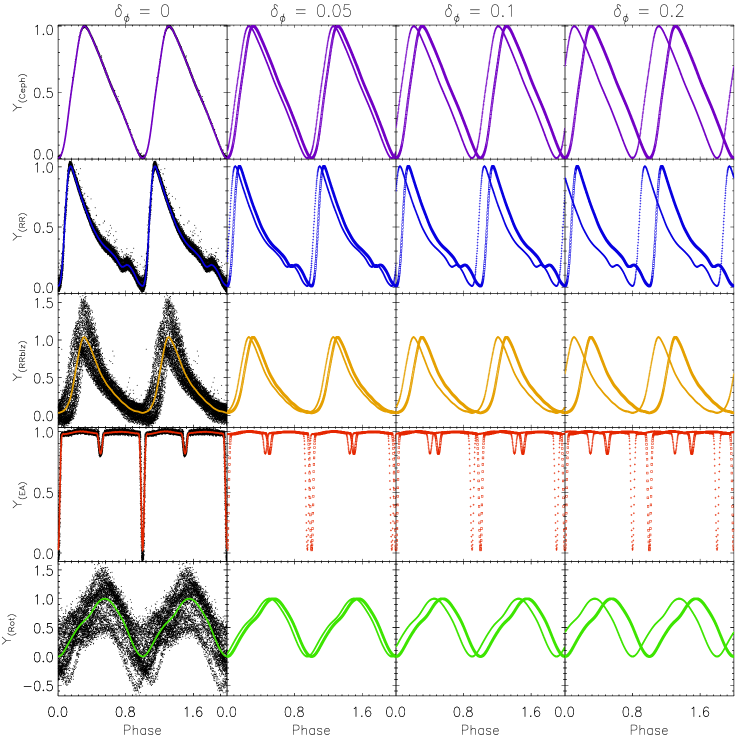
Figure 3: Ceph (purple - CoRoT-211626074), RR (blue - CoRoT-101370131), RRblz (yellow - CoRoT-100689962), EA (red - CoRoT-102738809), and Rot (green - CoRoT-110843734) phase diagrams. The dark dots in the first panels indicate the original data while the solid lines set the Fourier models $M(\phi)$. The next panels were build from the models where half of them are set by squares (measurements at $t>t_{0}+1./f$) and another half by crosses (measurements at $t>T_{tot}-1./f$). The frequencies used to build the phase diagram from left to right panels are $\mathrm{f_{true}+\delta f}$ to $\delta_{\phi}=[0,0.05,0.1,0.2]$, respectively.

4.1 Computing period and amplitude variations

Consider a generic light curve modeled by $Y\left(\phi\right)$ for $\left[\phi_{1},\phi_{2},\cdots,\phi_{N}\right]$ where $\phi_{i}$ are in ascending order. The tangent angles to the model can be written as

$$\theta_{i}=\arctan\left(\frac{Y\left(\phi_{i+1}\right)-Y\left(\phi_{i}\right)}{\phi_{i+1}-\phi_{i}}\right).$$ (14)

The angles are better to use than the $\alpha$ values to determine suitable regions to compute the period and amplitude variations because they can be assessed from the model without making any additional computation (see Sect. 4). The largest $\theta_{i}$ values are associated with the largest $\alpha$ values and the smallest $\theta_{i}$ values are associated with the smallest $\alpha$ values. The regions having smaller or bigger angles will be better to compute $\delta_{y}$ and $\delta_{\phi}$, respectively (see Sect. 4). After defining the region to compute these variations the following procedures should be performed:

• Calculate the amplitude variation ($\sigma_{y}$): consider the region(s) that enclose the majority of measurements having $\mathrm{|\theta|<\theta_{y}}$. Next for each $[\phi_{i}^{(o)},y_{i}^{(o)}]$ we find its respective $[\phi_{i}^{(m)},y_{i}^{(m)}]$ from which the vector $\delta_{y}=\left[y_{i}^{(o)}-y_{i}^{(m)},\cdots,y_{N}^{(o)}-y_{N`}^{(m)}\right]$ is obtained. Lastly, the amplitude variation is computed as

  $$\sigma_{y}=\gamma\times eMAD\left(\delta_{y_{i}}\right)$$ (15)

  where $\rm eMAD$ is the even-median absolute deviation of the even-median (Ferreira Lopes & Cross, 2017) and $\gamma$ is a correction factor (for more detail see Sect. 5.2.1). The $\rm eMAD$ is a slight modification to the $\rm MAD$ (the median absolute deviation of median). Indeed, $\sigma_{y}$ becomes a robust estimate of the standard deviation to outliers if $\gamma=1.48$ according to Hoaglin et al. (1983). A note of caution, $\delta_{y}$ is computed using $y_{i}^{(m)}$ instead of $y_{i}^{(e)}$ since the first one provides better estimations of expected values if the region cannot be well modeled by a line. Indeed, $y_{i}^{(m)}\simeq y_{i}^{(e)}$ only if $\theta_{i}\approx 0$.

• Calculate the period variation ($\sigma_{P}$): consider the region that encloses the majority of measurements having $\mathrm{|\theta|>\theta_{P}}$. For each $[\phi_{i}^{(o)},y_{i}^{(o)}]$ we find its respective $[\phi_{i}^{(e)},y_{i}^{(e)}]$, from which the vector $\delta_{\phi}=\left[\phi_{i}^{(o)}-\phi_{i}^{(e)},\cdots,\phi_{N}^{(o)}-\phi_{N}^{(e)}\right]$ is obtained. Lastly, the period variation is computed as

  $$\sigma_{P}=\gamma\times P\times eMAD\left(\delta_{\phi_{i}}\right).$$ (16)

The current approach estimates the period and amplitude uncertainties taking into account the variations about a model. Eqs. 15 and 16 are computed using only those measurements suitable to reduce the weight of either $\delta_{y}$ or $\delta_{\phi}$. However, the accuracy of $\sigma_{y}$ and $\sigma_{P}$ are extremely dependent on $\theta_{y}$ and $\theta_{P}$, respectively. For instance, values of $\theta=[0.1^{\circ},1^{\circ},5^{\circ},10^{\circ},70^{\circ},80^{\circ},89^{\circ},89.9^{\circ}]$ return $\alpha^{(\phi)}=[\sim 0.002,\sim 0.02,\sim 0.09,\sim 0.2,\sim 2.8,\sim 5.7,\sim 57,\sim 573]$. Indeed, the optimal choice of $\theta$ values is a compromise between the number of measurements enclosed for each limit and the usefulness of these measurements. Moreover, the statistical significance increases with the number of measurements while a higher signal-to-noise reduces the weight of $\delta_{y}$ on $\delta_{\phi}$. Therefore, the number of measurements and signal-to-noise are indirectly implicated in the period and amplitude variations.

5 Results and Discussion

Setting correct inputs using either method to select variable stars or to perform frequency finding searches is mandatory to get accurate outputs. The variability indices used to select variable stars candidates were studied deeply in the first two papers of this series, Ferreira Lopes & Cross (2016, 2017). These studies enabled us to provide the optimal constraints on noise models and establish well-defined criteria to settle the best approach to discriminate variable stars from noise as well as to affirm that the selection of a reliable sample is unfeasible using variability indices. Therefore, frequency analysis may also be used to select out untrustworthy variations but all constraints must be properly delimited and understood to avoid mistakes. For instance, the interquartile range can provide an incorrect list of variable star candidates if the time sampling is not taken into account. Therefore, all the relevant points about frequency finding methods were discussed in Sect. 1. The $\mathrm{f_{min}}$ and $\mathrm{f_{max}}$ are limited by the time series and the maximum reliable frequency, respectively. On the other hand, the sampling frequency was addressed in Sect. 2 in order to facilitate making a decision about the frequency resolution taking into account the effects on the frequency search. The frequency sampling and a new approach to computing period and amplitude variations are outlined in sections below.

Table 1: Constraints on the frequency search analysis performed by different surveys. The designation, $\mathrm{f_{min}}$, $\mathrm{f_{max}}$, mean total time span $\mathrm{\overline{T_{tot}}}$, and $\mathrm{N_{f}}$ of each survey are shown. The frequency unit is day${}^{-1}(d^{-1})$ and $\mathrm{\overline{T_{tot}}}$ is in days (d). Moreover, $\delta_{\phi}$ Eq.3 is given in the last column.

Survey	$\mathrm{f_{min}}(d^{-1})$	$\mathrm{f_{max}}(d^{-1})$	$\mathrm{\overline{T_{tot}}}(d)$	$\mathrm{N_{f}}$	$\delta_{\phi}$
CoRoT	$2/T_{tot}$	$3$	$\sim 136$	$2\times 10^{3}$	$0.20$
GAIA	$2/T_{tot}$	$3.9$	$\sim 1700$	$\sim 3\times 10^{3}$	$0.19$
Kepler	$\sim 3/T_{tot}$	$1$	$\sim 90$	$1300$	$0.07$
OGLE	$0$	$24$	$\sim 2780$	$10^{4}$	$>1$
TAROT1	$2/T_{tot}$	$f_{max}$	$\sim 900$	$10^{5}$	$\sim 0.22$
WFCAM2	$2/T_{tot}$	$f_{max}$	$\sim 1058$	$10^{5}$	$\sim 0.25$

• 1 - The frequency step is taken as described in Akerlof et al. (1994) and Larsson (1996).

• 2 - $f_{max}$ computed according to Eyer & Bartholdi (1999).

5.1 Optimal frequency sampling

An optimal determination of $\mathrm{f_{max}}$ is critical to reducing running time since it leads to the determination of the resolution and thus the number of frequencies or loops performed by the frequency finding algorithm (see Eq. 4). Estimation of $\mathrm{f_{max}}$ using the Nyquist frequency for oversampled data returns an overestimated frequency, i.e. frequencies that are this high are not reliably measured using the available data. Indeed, for unevenly and poorly sampled time series, the Nyquist frequency can be under or over-estimated whatever the estimation of the time interval from the measurements (as a mean or median value). For instance, long and short cadence CoRoT light curves have $\mathrm{f_{max}}$ of about $169d^{-1}$ and $2790d^{-1}$, respectively. These frequencies imply that the search for periodic variations at higher frequencies will not be productive. Therefore, empirical values have been adopted as the frequency limit. $\mathrm{f_{max}}=10d^{-1}$ has been generally adopted (e.g. Debosscher et al., 2007; Richards et al., 2012; De Medeiros et al., 2013) but higher values also can be found (e.g. Schwarzenberg-Czerny, 1996; Damerdji et al., 2007; Ferreira Lopes et al., 2015a). The parameters used to perform frequency searches for variable star catalogs for some surveys are listed in Table 1; the WFCAM multi-wavelength variable star catalog (WFCAM - Ferreira Lopes et al., 2015a), the Optical Gravitational Lensing Experiment (OGLE - Soszyński et al., 2009), the TAROT suspected variable star catalog (TAROT - Damerdji et al., 2007), GAIA data release 1 documentation, the semi-sinusoidal variables in the CoRoT mission (SR-CoRoT - De Medeiros et al., 2013), rotation periods of 12 000 main-sequence Kepler stars (Kepler - Nielsen et al., 2013), and the WFCAM multiwavelength Variable Star Catalog (WFCAM - Ferreira Lopes et al., 2015a). The $\mathrm{f_{max}}$ adopted by OGLE was used to estimate $\delta_{\phi}$ for the WFCAM and TAROT catalogs. Indeed, $\mathrm{f_{max}}$ values given by analytical expressions in Eyer & Bartholdi (1999) depend on each time series and such values are usually much higher than those empirically adopted.

The frequency sampling defined by Eq. 4 was designed without taking into account any particular criteria and hence this expression may work for any signal type. Indeed, the number of constraints is not reduced, but the frequency sampling given by shifts on the phase $\delta_{\phi}$ instead of shifts in frequency is clearer to read. Moreover, Eq. 3 also enables us to determine how much finer grain resolution is required to get a more accurate frequency estimation if the variability frequency is found since an initial value can be found with a coarser grain resolution. The frequencies not included in the frequency sampling may be detected or not, depending on the response to the frequency finding method for frequencies given by $\mathrm{f\pm\delta f/2}$, for instance. Indeed, the resolution of frequency sampling is critical for a large $T_{tot}$ since we find larger variations in the phase diagram for nearby frequencies. Moreover, as highlighted in previous sections, $\delta_{\phi}$ standardizes the criteria to perform frequency searches for time series having different total time spans. It allows us to compare straightforwardly the frequency analysis performed in different photometric surveys.

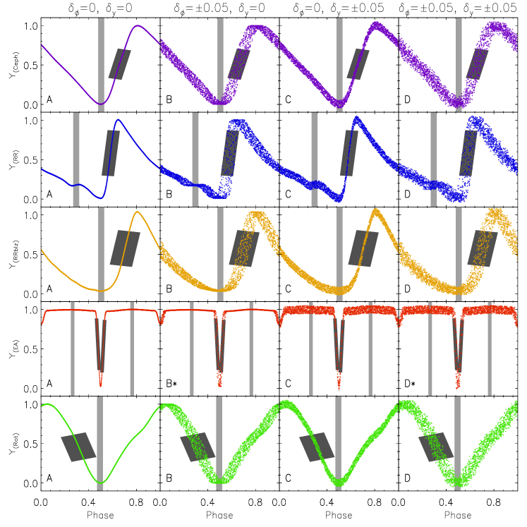
Figure 4: A single period (in contrast to Fig. 3 where two periods are shown) of the same models as shown in the Fig. 3. The phase diagrams were built assuming different values of $\delta_{\phi}$ and $\delta_{y}$ that are displayed at the top of each column of panels unless to EA $B*$ and $D*$ panels that was assumed a $\delta_{\phi}=0.025$. Indeed, the eclipse is missed for larger $\delta_{\phi}$ values. The regions used to compute the amplitude and period uncertainties are indicated by light grey and dark grey shading in all panels (for more details, see Sects. 4 and 5.3).

5.2 Visualizing frequency sampling effects

Consider a periodic signal of $1d^{-1}$ with measurements covering a variability cycle from $\mathrm{t=0}$ to $\mathrm{t=0+1/f}$ and another from $\mathrm{t=T_{tot}-1/f}$ to $\mathrm{t=T_{tot}}$. Five simulated time series that mimic pulsating stars ($Y_{(Ceph)}$, $Y_{(RR)}$, $Y_{(RRblz)}$), eclipsing binary stars ($Y_{(EA)}$), and rotational variables ($Y_{(Rot)}$) were chosen to illustrate our approach (for more details see Sect. 5.4). Figure 3 shows phase diagrams of simulated light curves where the first column of panels show the results for $\mathrm{f_{true}}$. The grey dots indicate the original light curve while the models are indicated by purple (Ceph), blue (RR), yellow (RRblz), red (EA), and green (Rot) colours. The measurements located at $\mathrm{t=0}$ to $\mathrm{t=0+1/f}$ are indicated by squares while those at $\mathrm{t=T_{tot}-1/f}$ to $\mathrm{t=T_{tot}}$ by crosses. The second, third, and fourth columns show phase diagrams using $\mathrm{f_{true}+\delta f}$ (see Eq. 3) for $\delta_{\phi}=[0.05,0.1,0.2]$, respectively. The crosses and squares limit the region where all measurements may be arranged considering that phase values computed at the beginning and end of the light curve set the largest variation from the model in the phase diagram as discussed in the Sect. 2. As one can see, the largest distortion of the model is found for binary stars, where the main variation is concentrated in a small part of the phase diagram. These aspects become increasingly important in the presence of noise or poorly sampled time series, when almost all measurements are required to adequately cover all variability phases. On the other hand, a low signal-to-noise is found for small frequency variations about $\mathrm{f_{true}}$ for those models where the variability is observed along the whole phase diagram like Ceph and RR. Indeed, the phase diagram dispersion is larger for those phenomena whose root variability causes period and/or amplitude variations like RRLyrae with the Blazhko effect (RRblz) and rotational variables (e.g. Buchler & Kolláth, 2011; Ferreira Lopes et al., 2015c). Indeed, non-radial pulsation, exoplanets, and different types of eclipsing and rotational variability enlarge the zoo of phase diagrams that can be produced by astrophysical phenomena (e.g. Prša et al., 2011; De Medeiros et al., 2013; Ferreira Lopes et al., 2015b; Paz-Chinchón et al., 2015).

To summarize, the phase diagrams of well-defined signals (fixed period and amplitude) only produce slight variations on the true frequency and hence these signals are easily identified compared to those ones with variable period or amplitude where the signal can be completely lost. Of course, the detection of these stars depends on the susceptibility to each frequency finding method. These matters will be addressed in a forthcoming paper of this project. The main conclusion provided by Eq. 4 is a clear limit to the variations in which a smooth phase diagram can be found.

5.2.1 Sorting out $\theta_{y}$, $\theta_{P}$, and correction factors

The same models described in the Sect. 5.2 were used to test our assumptions. Figure 4 shows the phase diagrams of five typical light curves where the A panels show the model; the B panels show a variation in the period with a constant amplitude; constant period with amplitude variation (C panels), and both amplitude and period variations (D panels). These variations were added to the model using a random uniform distribution, that mimics a non instrumental variation, while an instrumental variation may appear like a normal distribution. Indeed, the real non instrumental variation is more complicated and may include variations with normal, uniform and perhaps more complicated distributions. For instance, the RR and Rot models at the maximum seem to be composed of normal and uniform variations that are not necessarily symmetric about the model, indicating a more complex variation (see Fig. 3 first panels).

Eqs. 15 and 16 can be considered as a particular case where the noise or variation of amplitude or period is provided by a normal distribution since $1.48\times MAD$ is approximately the standard deviation value (Hoaglin et al., 1983). A uniform distribution has a different spread of values. Therefore, a correction factor ($\gamma$) may be considered in order to take account of the distribution type. The percentage of values of $68.27\%$, $95.45\%$ and $99.73\%$ that lie within a band around the mean of a normal distribution is given by $\gamma=1.48$, $\gamma=2.96$, and $\gamma=4.44$, respectively. However, $\gamma\simeq 1.37$, $\gamma\simeq 1.92$, and $\gamma\simeq 2.00$ contain the same fraction of values if an uniform distribution is considered. This factor improves our capability to measure an accurate estimation of the amplitude variation. For our simulation, this factor is not important since the ratio of computed and expected values are analysed (Sect. 5.3). On the other hand, $\gamma=1.48$ was used to estimate amplitude variation on real data (Sects. 5.4 and 5.5). The period and amplitude variations computed are given by the sum of intrinsic and acquired variations. Acquired variations are those which come from the environment or instrument while intrinsic variations come from the source itself. Indeed, low values for the uncertainties are limited by the instrument properties and for constraints related with observability like the sky background, noise from background sources, and blending. For instance, the period and amplitude variations can reveal particularities of phenomena observed if the acquired uncertainties can be deducted from a noise model (e.g. Cross et al., 2009; Aigrain et al., 2009; Ferreira Lopes & Cross, 2017). However the reliability of the period and amplitude variations measured will depend on the ratio $\delta_{\phi}/\delta_{y}$ as well as the regions used to compute them (see Sect. 4 for more detail).

Table 2: Angles ($\theta$) and angular coefficient ($\alpha$) values found for Ceph, RR, RRblz, EA, and Rot models. The angle limits $\theta_{y}$ and $\theta_{P}$ with their respective $\alpha_{y}$ and $\alpha_{\phi}$ values used to set the regions to compute the period and amplitude variations as well as the maximum angle found in each model are displayed below.

Model	$\mid\theta\mid_{max}$	$\theta_{y}$	$\mid\alpha_{y}\mid$	$\theta_{P}$	$\mid\alpha_{\phi}\mid$
Ceph	$79.02^{o}$	$31.05^{o}$	$0.18$	$76.73^{o}$	$4.68$
RR	$85.52^{o}$	$28.77^{o}$	$0.37$	$83.67^{o}$	$10.99$
RRblz	$81.30^{o}$	$18.94^{o}$	$0.10$	$76.25^{o}$	$4.74$
EA	$88.39^{o}$	$7.87^{o}$	$0.04$	$87.94^{o}$	$32.00$
Rot	$74.82^{o}$	$34.87^{o}$	$0.20$	$72.90^{o}$	$3.48$

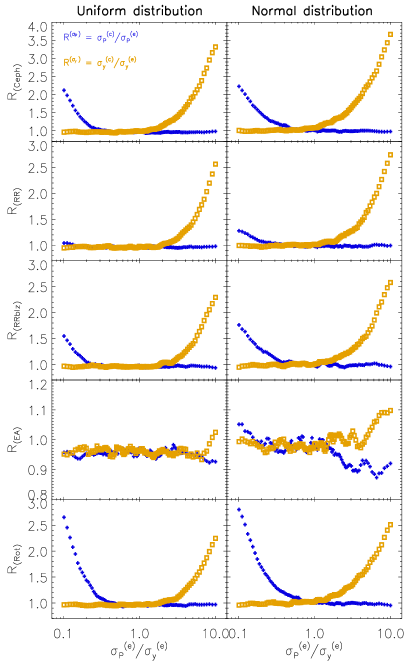
Figure 5: The ratio of computed and expected uncertainty values for period ($R^{(\sigma_{P})}$ - blue crosses) and amplitude ($R^{(\sigma_{y})}$ - yellow squares) as function of $\mathrm{\sigma_{P}^{(e)}/\sigma_{y}^{(e)}}$ for EA, RRblz, RR, Ceph, and Rot models. The results where the noise was introduced using an uniform and normal distribution are displayed in the left and right panels, respectively.

5.3 Testing frequency uncertainities

The models described in Sect. 5.2 (see A panels of Fig. 3) were used to perform the simulations. The regions chosen to compute the amplitude and period uncertainties are shown in Fig. 4. The measurements in these regions have angles within the defined angle limits which were set to best compute the uncertainties (see Sect. 4 for more details). Indeed, on average the maximum angle values are reduced and the minimum angle values are increased when the noise contribution is increased. Table 2 shows the main parameters values found in each model. Next, $10^{6}$ Monte Carlo simulations were performed setting $\mathrm{\sigma_{P}^{(e)}/\sigma_{y}^{(e)}}$ in the range from $0.1$ to $10$. $\mathrm{\sigma_{P}^{(e)}}$ and $\mathrm{\sigma_{y}^{(e)}}$ were introduced using a uniform distribution or a normal distribution. Finally, the amplitude and period uncertainties were computed according to Eqs. 15 and 16. The ratio of the computed and expected uncertainty values for period ($R^{(\sigma_{P})}$) and amplitude ($R^{(\sigma_{y})}$) were used to estimate the reliability of computed values. Figure 5 shows the main results obtained in the simulations, which are summarized below;

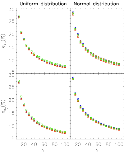
Figure 6: Percent relative error for $\sigma_{P}$ and $\sigma_{y}$ as a function of the number of measurements using an uniform (left panels) and a normal (right panels) distribution. The colours indicate the result for different models in the same way as Figs. 3 and 4.

• The results found using uniform and normal distributions are quite similar except for EA models. This happens because the eclipse is ”missed” more quickly when the uncertainty is introduced by normal distributions than with uniform distributions. Considering the same sigma value for both distributions, a normal distribution of errors provides a larger dispersion of simulations than an uniform distribution. For instance, $\sim 4.44\times eMAD$ is required to enclose $\sim 99.7\%$ of observed measurements for a normal distribution while $\sim 2.00\times eMAD$ is required for a uniform distribution (see Sect. 5.2.1).

• $R^{(\sigma_{P})}\simeq R^{(\sigma_{y})}\simeq 1$ is found for $\mathrm{\sigma_{P}^{(e)}/\sigma_{y}^{(e)}}$ ranging from $\sim 0.5$ to $\sim 2$ for all models as well as for both uniform and normal distributions. Indeed, the EA model has $R^{(\sigma_{P})}\simeq R^{(\sigma_{y})}\simeq 1$ for almost all values of the ratio. $\alpha_{y}$ is smaller than $0.1$ while $\alpha_{\phi}$ is bigger than $10$ for EA model and hence the weight of $\mathrm{\sigma_{P}^{(e)}/\sigma_{y}^{(e)}}$ on the computed uncertainties is reduced (see Table 2).

• The greatest difference between computed and expected values (R) are found at extreme ratios, i.e those regions where $\mathrm{\sigma_{P}^{(e)}>>\sigma_{y}^{(e)}}$ or $\mathrm{\sigma_{P}^{(e)}<<\sigma_{y}^{(e)}}$.

  

  

  

  

  

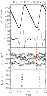
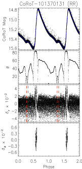
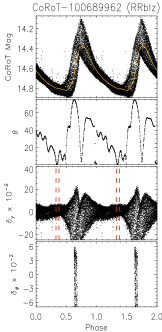
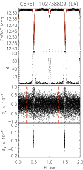
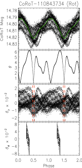
  Figure 7: Ceph (purple - CoRoT-211626074), RR (blue - CoRoT-101370131), RRblz (yellow - CoRoT-100689962), EA (red - CoRoT-102738809), and Rot (green - CoRoT-110843734) phase diagrams in normalized flux shown in the top row of panels. The angles found for each models (second row of panels), the $\delta_{y}$ (third row of panels), and $\delta_{\phi}$ values (bottom row of panels) are also shown. Indeed, the last panel only show the results for the region used to compute the period variation.

  Table 3: Parameters for CoRoT stars used to test the approach proposed in this work. The L indicate the parameters obtained in the literature which the references for are indicated in the last column. Indeed, the values of Ra, Dec, R magnitude, and the exposure time ($T_{exp}$) were obtained from the CoRoT database.

  CoRoT-ID	Var. Type	RA	DEC	R	$\sigma_{(2h)}$	$P_{(L)}(d)$	$\delta P(d)$	$T_{exp}(d)$	$A_{(L)}(mag)$	$eA_{(L)}(mag)$	Ref
  211626074	Ceph	285.469	3.277	$12.60$	$1.41\times 10^{-4}$	$5.470600$	$\cdot$	$5.93\times 10^{-3}$	$2.96\times 10^{-1}$	$1.44\times 10^{-3}$	$1$
  101370131	RR	292.060	0.101	$15.28$	$6.60\times 10^{-4}$	$6.19332\times 10^{-1}$	$\cdot$	$5.93\times 10^{-3}$	$\cdot$	$\cdot$	$2$
  100689962	RRblz	291.000	1.697	$14.65$	$4.60\times 10^{-4}$	$3.55997\times 10^{-1}$	$\cdot$	$5.93\times 10^{-3}$	$\cdot$	$\cdot$	$3$
  102738809	EA	101.131	0.832	$12.29$	$1.18\times 10^{-4}$	$2.035701$	$\cdot$	$3.70\times 10^{-4}$	$\cdot$	$\cdot$	$4$
  110843734	Rot	102.918	-3.748	$14.81$	$5.03\times 10^{-4}$	$8.186000$	$4.94\times 10^{-2}$	$5.93\times 10^{-3}$	$5.66\times 10^{-2}$	$1.42\times 10^{-2}$	$5$

  • The last column is regarding to the references that provided the following parameters above; (1) Poretti et al. (2015), (2) Paparó et al. (2009) (3) Chadid et al. (2010), (4) Maciel et al. (2011); Carone et al. (2012) (5) De Medeiros et al. (2013). Moreover, the noise level ($\sigma_{2h}$) were computed using the Eq. 1 described by Aigrain et al. (2009) where z was computes as the mean value of CoRoT Run analysed by the authors.

• The discussion above can be summarized if the Eqs. 11 and 13 are extrapolated thus:

  $$R^{(\sigma_{y})}=\frac{\sigma_{y}^{(c)}}{\sigma_{y}^{(e)}}\simeq\left|\alpha_{y}\right|\times\frac{\sigma_{P}^{(e)}}{\sigma_{y}^{(e)}}+1$$ (17)

  and

  $$R^{(\sigma_{P})}=\frac{\sigma_{P}^{(c)}}{\sigma_{P}^{(e)}}\simeq\left|\alpha_{\phi}^{-1}\right|\times\left(\frac{\sigma_{P}^{(e)}}{\sigma_{y}^{(e)}}\right)^{-1}+1.$$ (18)

  $R^{(\sigma_{y})}$ and $R^{(\sigma_{P})}$have opposite behaviour since they vary with $\mathrm{(\sigma_{P}^{(e)}/\sigma_{y}^{(e)}})^{\pm 1}$, respectively. $R^{(\sigma_{y})}$ implies a rational function if $\mathrm{\sigma_{P}^{(e)}/\sigma_{y}^{(e)}}$ has values smaller than $1$ while the opposite is found for $R^{(\sigma_{P})}$. However, both functions depend on an angular coefficient ($\left|\alpha_{y}\right|$ or $\left|\alpha_{P}\right|$) that will determine the trend variation.

The simulations are in agreement with the analysis in Sect. 4. The amplitude and period variations can bias the uncertainty estimations of one another, mainly when $\mathrm{\sigma_{P}^{(e)}/\sigma_{y}^{(e)}}<<1$ or $\mathrm{\sigma_{P}^{(e)}/\sigma_{y}^{(e)}}>>1$. Indeed, Eqs. 17 and 18 can be used to estimate the reliability of uncertainties if $\mathrm{\sigma_{P}^{(e)}/\sigma_{y}^{(e)}}$ can be estimated somehow.

The relative errors of the uncertainties were also analysed as function of the number of measurements (see Fig. 6). As result, a decrease in the error with the number of measurements is found, as expected. This means that the number of measurements is an implicit parameter in Eqs. 15 and 16 that improve the statistic significance of uncertainties.

5.4 Describing Models and Testing the Approach on Observed Data

Ceph, RR, RRblz, EA, and Rot models were based on the CoRoT light curves CoRoT-211626074, CoRoT-101370131, CoRoT-100689962, CoRoT-102738809, and CoRoT-110843734, respectively. The variability types were previously identified by Debosscher et al. (2007); Poretti et al. (2015); Paparó et al. (2009); Chadid et al. (2010); Maciel et al. (2011); Carone et al. (2012) and De Medeiros et al. (2013). Table 3 shows the main parameters of these sources that were obtained in the literature (L). These light curves were modeled using a harmonic fit with $12$, $12$, $12$, $24$, and $4$ harmonics for $Ceph$, $RR$, $RRblz$, $EA$, and $Rot$ variable stars, respectively. Higher number of harmonics can be used, however this also increases the processing time necessary to model and to perform simulations. The $Y_{(RRblz)}$ and $Y_{(Rot)}$ variable stars present variations in the amplitude and a period-amplitude variation. The $Y_{(RRblz)}$ has a Blazhko effect that is a long-period modulation or a variation in period and amplitude of RR Lyrae stars (e.g. Szabó, 2014). On the other hand, the $Y_{(Rot)}$ displays amplitude variation due the to the magnetic activity cycles and period variation due to differential rotation (e.g. Ferreira Lopes et al., 2015c; Das Chagas et al., 2016). The exposure time ($T_{exp}$) provided by CoRoT mission and the empirical noise relation ($\sigma_{2h}$) described by Aigrain et al. (2009) were used to analysis the period and amplitude variation.

The tests performed in the sections 4, 5.2, and 5.2.1 used models scaled to unit amplitude. It is useful to test our approaches for different signal types. For instance, the Ceph, RR, RRblz, EA, EB and Rot models have similar angles (see Table 2) but a wide difference among them is found when the real data is considered (see Fig. 7) since they have different typical amplitudes. Therefore, the angles found in the real data are not the same as those found for the models tested in the previous sections, as expected. These variations occur because $\tan(\theta)=\delta y/\delta\phi$, i.e. a bigger $\delta y$ for the same $\delta\phi$ implies a larger angle. Figure 7 shows the CoRoT light curves (first row of panels), the angles as a function of phase along the light curve (second row of panels), the observed minus modeled values (third row of panels), and finally the $\delta\phi$ values for the region used do compute the period variation. For example, the $\theta_{max}$ for $Rot$ models is about twelve times bigger than those found when amplitude is scaled to unit amplitude. On the other hand, the $\theta_{max}$ of the Ceph, RR, RRblz, EA, and EB decrease by factors smaller than $0.5$.

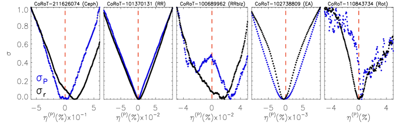
Figure 8: The normalized standard deviation scaled between 0 and 1 as function of the percent relative error of $P_{L}$. The results for the residuals and period are shown as black and blue dots, respectively. The red line sets the location of the variability period determined in literature $P_{(L)}$.

Table 4: Parameters for CoRoT stars computed from the aproaches proposed in this work.

CoRoT-ID	$P(d)$	$\delta P_{(FWHM)}^{(LSG)}(d)$	$\delta P_{(FWHM)}^{(STR)}(d)$	$\sigma_{P}(d)$	$A(mag)$	$\sigma_{A}(mag)$	$\sigma_{r}(mag)$	$\sigma_{P}/\sigma_{A}$	$Log(T_{tot}/P)$
211626074	$5.47073174$	$4.55\times 10^{-1}$	$3.33\times 10^{-1}$	$5.27\times 10^{-3}$	$2.99\times 10^{-1}$	$1.58\times 10^{-3}$	$1.87\times 10^{-3}$	$2.86$	$6.69\times 10^{-1}$
101370131	$6.19331408\times 10^{-1}$	$9.15\times 10^{-4}$	$7.46\times 10^{-4}$	$5.80\times 10^{-4}$	$7.98\times 10^{-1}$	$7.53\times 10^{-3}$	$8.14\times 10^{-3}$	$0.06$	$2.39$
100689962	$3.56090879\times 10^{-1}$	$3.27\times 10^{-4}$	$2.93\times 10^{-4}$	$2.23\times 10^{-2}$	$4.50\times 10^{-1}$	$3.82\times 10^{-2}$	$6.19\times 10^{-2}$	$0.52$	$2.60$
102738809	$2.03569293$	$1.17\times 10^{-2}$	$3.02\times 10^{-3}$	$7.02\times 10^{-4}$	$3.30\times 10^{-1}$	$3.47\times 10^{-3}$	$3.52\times 10^{-3}$	$0.25$	$1.81$
110843734	$8.21895695$	$1.74\times 10^{-1}$	$1.70\times 10^{-1}$	$1.71\times 10^{-1}$	$2.68\times 10^{-2}$	$6.06\times 10^{-3}$	$7.76\times 10^{-3}$	$30.01$	$1.13$

Figure 7 displays, step by step, the procedure that must be used to compute period and amplitude variations: the variability period is computed and the light curve is folded; next, a model is obtained using harmonic fits (see solid lines in the upper panels); from the models the angles are determined (see second row of panels) from where the regions used to compute period and amplitude variations are established; the amplitude variation is given by the standard deviation of the residuals in the region of phase diagram where $\left|\theta\right|<\theta_{y}$; and the period variation is found by multiplying the variability period by $eMAD$ of $\delta_{\phi}^{(c)}$ (given by Eq. 16). The periods and amplitudes as well as their uncertainties and variations were computed as described in Sect. 4.1 (see Table 4). The results were compared with previous ones (see Table 3) where the main remarks are summarized below;

• The period that leads to the smallest $\sigma_{P}$ is not always related with the smallest $\sigma_{r}$ (see Fig. 8).

• All $\sigma_{A}$ values are bigger than those given by $\sigma_{2h}$. This indicates an underestimation of $\sigma_{2h}$ or that all sources have an intrinsic amplitude variation. A note of caution, the noise values decrease with $Log(T_{tot}/P)$ and hence such a comparison cannot be performed straightforwardly.

• CoRoT-100689962, CoRoT-110843734, and CoRoT-102738809 have $\sigma_{P}$ values larger than the exposure time ($T_{exp}$). However, CoRoT-101370131 has $\sigma_{P}$ ten times smaller than $T_{exp}$.

• The $\sigma_{P}/\sigma_{A}$ values for all sources are smaller than $\sim 0.5$ or bigger than $2$ (see Sect. 5.3). It indicates that all $\sigma_{P}$ and $\sigma_{A}$ values are biased by amplitude or period variation, respectively. Indeed, the intrinsic variation is not known a priori and hence the information provided by the ratio $\sigma_{P}/\sigma_{A}$ will only be accurate if $\mid\alpha_{y}\mid<<0$ and $\mid\alpha_{\phi}\mid>>1$ (see Sect. 4).

• The variability periods determined by us are in agreement with those found in the literature. Indeed, the literature periods are determined as the highest power spectrum peak while those found by us are calculated by minimising $\sigma_{P}$.

• The period uncertainty $\delta P_{(FWHM)}^{(STR)}$ method is always smaller than $\delta P_{(FWHM)}^{(LSG)}$ that indicates that STR is more sensitive to variation in the phase diagram than the LSG method.

• CoRoT-211626074 - The amplitude ($A_{(L)}$) found in the literature is about $1\%$ smaller than that found by us. However, the authors used the DR2 release while our data come from the DR4 release. Indeed, the amplitudes are in agreement within the error bars. The $\sigma_{A}$ is at least nine times bigger than $\sigma_{2h}$. Moreover, $\sigma_{P}/\sigma_{A}=2.86$ indicates that the weight of $\sigma_{P}$ in $\sigma_{A}$ is not strong, and vice-versa. It indicates that some of the amplitude variation comes from the sources. This result is supported by the detection of overtone pulsation reported by Poretti et al. (2015). Indeed, the determination of amplitude variation reported by us was only settled by determination of $\sigma_{A}$ while the authors use complex analysis.

• CoRoT-101370131 - The $\sigma_{P}$ is smaller than $T_{exp}$ indicating a non-intrinsic variation related with the period. On the other hand, the amplitude variation $\sigma_{A}$ is about nine times bigger than $\sigma_{2h}$. Moreover, $\sigma_{P}/\sigma_{A}=0.06$ also indicates that $\sigma_{A}$ is not biased by $\sigma_{P}$. Therefore, an intrinsic variation of the CoRoT-101370131 can be real if the noise level estimation is reliable.

• CoRoT-100689962 - The period and amplitude variation is clearly observed in the phase diagram. Moreover, it has the largest $Log(T_{tot}/P)$ and hence the smallest $\delta P_{(FWHM)}$ in agreement with the discussion performed in Sect. 3. Moreover, $\sigma_{P}/\sigma_{A}=0.52$ indicates that the period variation is not strongly biased by amplitude variation and vice-versa. Therefore, the $\sigma_{P}$ and $\sigma_{A}$ mean that intrinsic variations come from the source since these variations are $\sim 3.8$ times bigger than $T_{exp}$ and $\sim 12$ times bigger than $\sigma_{2h}$, respectively.

• CoRoT-102738809 - The $\sigma_{P}$ is the smallest value among the sources analysed. Indeed, this aspect is caused by the large angles and the shape of the light curve. Moreover, this source has the shortest exposure time (see Table 3). The $\sigma_{P}$ does not show strong evidence of a period variation since it is smaller than twice $T_{exp}$. On the other hand, $\sigma_{A}$ is three times larger than $\sigma_{2h}$ that indicates a small intrinsic variation related with the amplitude. Indeed, the region used to compute the amplitude variation is related with the eclipse phase where both stars are side by side. Therefore, $\sigma_{A}$ can be related to one or both stars.

• CoRoT-110843734 - The $\delta P_{(FWHM)}$ is bigger than $\delta P$ and hence the empirical relation given by Lamm et al. (2004) can provide values smaller than those found for the $\delta P_{(FWHM)}$ estimations. $A_{(L)}$ is about twice that estimated by us. Such a difference can only be achieved by a typing error. On the other hand, the period computed by the authors is in agreement with that found for us. $\theta_{max}\sim 6^{o}$ and hence the period variation is biased by amplitude variation. Indeed, $\sigma_{P}/\sigma_{A}=30.0$ indicates an unreliable estimation of $\sigma_{P}$ using the phase diagram. Therefore, $\sigma_{P}$ or $\sigma_{A}$ are not useful as indicators of intrinsic variation for rotational variables having small amplitudes. However, the estimation of period and amplitude variation with time instead of phase can reveal important clues about stellar activity cycles (e.g. Ferreira Lopes et al., 2015c).

In summary, the period and amplitude variation can provide important information about the intrinsic variation of the source. However, it is trustworthy only if $\theta_{max}>>\theta_{min}$ since the capability to discriminate period and amplitude variation decreases. For a complete characterization of a light curve the period uncertainty as well as period variation must be determined.

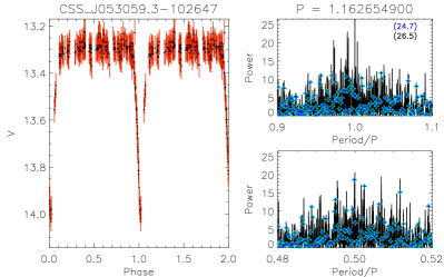
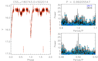
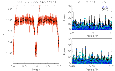
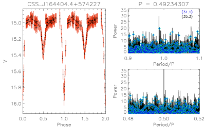
Figure 9: Phase diagram of 4 $EA_{up}$ Catalina stars where we also display the Lomb-Scargle periodogram about the variability period (top right panel for each star) and about half the variability period (bottom right panel for each star). The name and the variability period is shown in each diagram. The solid black line shows the power spectrum considering a number of frequencies obtained from Eq.4 assuming $\delta_{\phi}=0.01$ while those values found using $N_{freq}=10^{4}$ are marked by blue crosses. Moreover, the maximum power found for both methods of frequency sampling is displayed in the upper right corner.

5.5 Testing Frequency Sampling on Observed Data

The Catalina Real Time Survey found about $\sim 47000$ periodic variables stars in Data Release-1 (Drake et al., 2014). The authors reported a sample of EA variables stars where the period determination was not possible due an insufficient number of observations at the eclipses. These stars were reported as EA variables having unknown-period ($EA_{up}$). The Lomb-Scargle method (Lomb, 1976; Scargle, 1982) was used to perform a period search but the frequency range and frequency sampling are not given by the authors. Therefore, a mean value of those shown in the Table 1 were assumed, i.e. $F_{min}=2/T_{tot}$, $F_{max}=10$, and $N_{freq}=10^{4}$. These constraints were assumed as those used by the authors to review a small sample of $EA_{up}$ stars.

Indeed, EA stars require a high frequency sampling to allow us to determine the variability period otherwise the eclipse region will not be smoothly folded (see $Y_{(EA)}$ panel Fig. 3). Section 2 discussed the frequency sampling in detail where the $\delta_{\phi}$ required to find the variability periods for EA stars is smaller than $0.05$ in order to be able to fold the eclipse properly. Therefore, four $EA_{up}$ Catalina stars (see Table 5) were reviewed using the frequency sampling given by $\delta_{\phi}=0.01$. Indeed, the sample analysed has $T_{tot}\simeq 3000$ days that implies a number of frequencies $\sim 3\times 10^{6}$ (see Eq.4).

Figure 9 shows four $EA_{up}$ stars where the variability period was determined. In the right panel of each phase diagram is shown the Lomb-Scargle power spectrum about the variability period using $N_{freq}=10^{4}$ (blue crosses) and a number of frequencies obtained from Eq.4 assuming $\delta_{\phi}=0.01$ and $F_{max}=10$. As one can verify the highest peak of the black lines is related to the maximum power of the periodogram. On the other hand, these peaks are not found when the sampling frequency is reduced (blue crosses). Therefore, the variability periods of $EA_{up}$ stars were not identified due to low frequency sampling. The main parameters of the four $EA_{up}$ stars analysed in the present work are presented in the Table 5.

Table 5: Parameters for $EA_{up}$ Catalina stars computed from the approaches proposed in this work.

Catalina-ID	$P(d)$	$\delta P_{(FWHM)}^{(LSG)}(d)$	$\delta P_{(FWHM)}^{(STR)}(d)$	$\sigma_{P}$	V	$A$	$\sigma_{A}$	$\sigma_{R}$	$Log(T_{tot}/P)$
CSS_J053059.3-102647	$1.16265491$	$1.32\times 10^{-4}$	$7.69\times 10^{-5}$	$2.08\times 10^{-3}$	$13.350$	$7.50\times 10^{-1}$	$2.83\times 10^{-2}$	$2.17\times 10^{-2}$	$3.40$
CSS_J180743.0+502014	$9.92055466\times 10^{-1}$	$8.20\times 10^{-5}$	$6.99\times 10^{-5}$	$1.22\times 10^{-3}$	$15.810$	$1.14$	$2.71\times 10^{-2}$	$1.09\times 10^{-1}$	$3.49$
CSS_J090355.3+533131	$3.31637448\times 10^{-1}$	$1.33\times 10^{-5}$	$2.49\times 10^{-5}$	$2.27\times 10^{-3}$	$15.095$	$6.32\times 10^{-1}$	$2.06\times 10^{-2}$	$3.01\times 10^{-2}$	$3.94$
CSS_J164404.4+574227	$4.92343069\times 10^{-1}$	$1.14\times 10^{-5}$	$4.56\times 10^{-5}$	$1.18\times 10^{-3}$	$15.088$	$9.92\times 10^{-1}$	$1.64\times 10^{-2}$	$2.91\times 10^{-2}$	$3.74$

Indeed, from a methodology viewpoint, the identification of variability periods of $EA_{up}$ stars requires a suitable period finding method and high frequency sampling (see Sect. 2) to detect the signal. Moreover, the susceptibility of the period finding methods varies for different signal shapes (see Fig. 3). Therefore, a deeper analysis of all $EA_{up}$ stars will be performed in a forthcoming paper where other methods besides Lomb-Scargle will also be used. As a result, we will define limits on what constitutes an insufficient number of observations.

6 Conclusions

Frequency analysis constraints as well as the period and amplitude variations were analysed in the present work. A new approach to compute frequency sampling was introduced. This analysis is fundamental to providing a precise number of frequencies required to perform period finding searches. It also enables us to identify optimal values for searching for particular variable types as well as how much resolution is required to increase the accuracy of the periods found. We consider that this approach is fundamental to efficiently face the challenges of big data science since analytical equations are imposed.

The period and amplitude variation of light curves were also reviewed. We show that a complete characterization of a light curve requires separating period uncertainty and period variation, from which important information about the variability nature can be estimated. On the other hand, the noise and amplitude variation also provide new clues about intrinsic variations that come from the source. The analyses performed in this project are very useful since all aspects of the analyses of large photometric surveys are being studied in order to maximize the probability of finding variable stars, reduce the running time, and reduce the number of misclassifications. The current paper is the second step towards unbiased samples, i.e. samples that only enclose reliable variations since this is unfeasible using correlated or non-correlated indices alone. Moreover, in this project we try to standardize the analysis criteria for variable stars in photometric surveys. In spite of this, the dependence of variability indices on the instrumental properties has been reduced and now, we also propose an estimation of frequency sampling that reduces the dependence on the total time span or time sampling of the data. Moreover, an approach to study the amplitude and period variation is presented. We consider that these estimations provide better information about the phenomena observed than previous ones since these estimations are limited by instrument properties or signal features. These must be taken into account for a realistic estimation.

This paper concludes our studies about the constraints used to perform frequency searches. A new frequency finding method and new insights to detect aperiodic variations and to determine the false alarm probability will be addressed in a forthcoming paper of this series.

References

- Aigrain et al. (2009) Aigrain S., et al., 2009, A&A, 506, 425
- Akerlof et al. (1994) Akerlof C., et al., 1994, ApJ, 436, 787
- Baglin et al. (2007) Baglin A., Auvergne M., Barge P., Michel E., Catala C., Deleuil M., Weiss W., 2007, in Dumitrache C., Popescu N. A., Suran M. D., Mioc V., eds, American Institute of Physics Conference Series Vol. 895, Fifty Years of Romanian Astrophysics. pp 201–209, doi:10.1063/1.2720423
- Bailer-Jones et al. (2013) Bailer-Jones C. A. L., et al., 2013, A&A, 559, A74
- Borucki et al. (2010) Borucki W. J., et al., 2010, Science, 327, 977
- Bravo et al. (2014) Bravo J. P., Roque S., Estrela R., Leão I. C., De Medeiros J. R., 2014, A&A, 568, A34
- Buchler & Kolláth (2011) Buchler J. R., Kolláth Z., 2011, ApJ, 731, 24
- Carone et al. (2012) Carone L., et al., 2012, A&A, 538, A112
- Chadid et al. (2010) Chadid M., et al., 2010, A&A, 510, A39
- Cross et al. (2009) Cross N. J. G., Collins R. S., Hambly N. C., Blake R. P., Read M. A., Sutorius E. T. W., Mann R. G., Williams P. M., 2009, MNRAS, 399, 1730
- Damerdji et al. (2007) Damerdji Y., Klotz A., Boër M., 2007, AJ, 133, 1470
- Das Chagas et al. (2016) Das Chagas M. L., et al., 2016, MNRAS, 463, 1624
- De Medeiros et al. (2013) De Medeiros J. R., et al., 2013, A&A, 555, A63
- Debosscher et al. (2007) Debosscher J., Sarro L. M., Aerts C., Cuypers J., Vandenbussche B., Garrido R., Solano E., 2007, A&A, 475, 1159
- Distefano et al. (2012) Distefano E., Lanzafame A. C., Lanza A. F., Messina S., Korn A. J., Eriksson K., Cuypers J., 2012, MNRAS, 421, 2774
- Drake et al. (2014) Drake A. J., et al., 2014, ApJS, 213, 9
- Dubath et al. (2011) Dubath P., et al., 2011, MNRAS, 414, 2602
- Dworetsky (1983) Dworetsky M. M., 1983, MNRAS, 203, 917
- Eyer (2006) Eyer L., 2006, in Aerts C., Sterken C., eds, Astronomical Society of the Pacific Conference Series Vol. 349, Astrophysics of Variable Stars. p. 15 (arXiv:astro-ph/0511458)
- Eyer & Bartholdi (1999) Eyer L., Bartholdi P., 1999, A&AS, 135, 1
- Ferreira Lopes & Cross (2016) Ferreira Lopes C. E., Cross N. J. G., 2016, A&A, 586, A36
- Ferreira Lopes & Cross (2017) Ferreira Lopes C. E., Cross N. J. G., 2017, A&A, 604, A121
- Ferreira Lopes et al. (2015a) Ferreira Lopes C. E., Dékány I., Catelan M., Cross N. J. G., Angeloni R., Leão I. C., De Medeiros J. R., 2015a, A&A, 573, A100
- Ferreira Lopes et al. (2015b) Ferreira Lopes C. E., et al., 2015b, A&A, 583, A122
- Ferreira Lopes et al. (2015c) Ferreira Lopes C. E., Leão I. C., de Freitas D. B., Canto Martins B. L., Catelan M., De Medeiros J. R., 2015c, A&A, 583, A134
- Foster (1996) Foster G., 1996, AJ, 112, 1709
- Graham et al. (2013) Graham M. J., Drake A. J., Djorgovski S. G., Mahabal A. A., Donalek C., Duan V., Maker A., 2013, MNRAS, 434, 3423
- Gregory (2001) Gregory P. C., 2001, in Mohammad-Djafari A., ed., American Institute of Physics Conference Series Vol. 568, Bayesian Inference and Maximum Entropy Methods in Science and Engineering. pp 557–568, doi:10.1063/1.1381917
- Heck et al. (1985) Heck A., Manfroid J., Mersch G., 1985, A&AS, 59, 63
- Hoaglin et al. (1983) Hoaglin D. C., Mosteller F., Tukey J. W., 1983, Understanding robust and exploratory data anlysis. New York: John Wiley
- Huijse et al. (2011) Huijse P., Estevez P. A., Zegers P., Principe J. C., Protopapas P., 2011, IEEE Signal Processing Letters, 18, 371
- Huijse et al. (2012) Huijse P., Estevez P. A., Protopapas P., Zegers P., Principe J. C., 2012, IEEE Transactions on Signal Processing, 60, 5135
- Ivezic et al. (2008) Ivezic Z., et al., 2008, Serbian Astronomical Journal, 176, 1
- Kato & Uemura (2012) Kato T., Uemura M., 2012, PASJ, 64, 122
- Kovacs (1981) Kovacs G., 1981, Ap&SS, 78, 175
- Lamm et al. (2004) Lamm M. H., Bailer-Jones C. A. L., Mundt R., Herbst W., Scholz A., 2004, A&A, 417, 557
- Lanza et al. (2014) Lanza A. F., Das Chagas M. L., De Medeiros J. R., 2014, A&A, 564, A50
- Larsson (1996) Larsson S., 1996, A&AS, 117, 197
- Lomb (1976) Lomb N. R., 1976, Ap&SS, 39, 447
- Maciel et al. (2011) Maciel S. C., Osorio Y. F. M., De Medeiros J. R., 2011, New Astron., 16, 68
- Minniti et al. (2010) Minniti D., et al., 2010, New Astron., 15, 433
- Nielsen et al. (2013) Nielsen M. B., Gizon L., Schunker H., Karoff C., 2013, A&A, 557, L10
- Oluseyi et al. (2012) Oluseyi H. M., et al., 2012, AJ, 144, 9
- Paparó et al. (2009) Paparó M., Szabó R., Benkő J. M., Chadid M., Poretti E., Kolenberg K., Guggenberger E., Chapellier E., 2009, in Guzik J. A., Bradley P. A., eds, American Institute of Physics Conference Series Vol. 1170, American Institute of Physics Conference Series. pp 240–244, doi:10.1063/1.3246453
- Paz-Chinchón et al. (2015) Paz-Chinchón F., et al., 2015, preprint, (arXiv:1502.05051)
- Poretti et al. (2015) Poretti E., Le Borgne J. F., Rainer M., Baglin A., Benkő J. M., Debosscher J., Weiss W. W., 2015, Monthly Notices of the Royal Astronomical Society, 454, 849
- Prša et al. (2011) Prša A., et al., 2011, AJ, 141, 83
- Reimann (1994) Reimann J. D., 1994, PhD thesis, UNIVERSITY OF CALIFORNIA, BERKELEY.
- Reinhold & Gizon (2015) Reinhold T., Gizon L., 2015, A&A, 583, A65
- Reinhold et al. (2013) Reinhold T., Reiners A., Basri G., 2013, A&A, 560, A4
- Richards et al. (2011) Richards J. W., et al., 2011, ApJ, 733, 10
- Richards et al. (2012) Richards J. W., Starr D. L., Miller A. A., Bloom J. S., Butler N. R., Brink H., Crellin-Quick A., 2012, VizieR Online Data Catalog, 220
- Scargle (1982) Scargle J. D., 1982, ApJ, 263, 835
- Schwarzenberg-Czerny (1989) Schwarzenberg-Czerny A., 1989, MNRAS, 241, 153
- Schwarzenberg-Czerny (1996) Schwarzenberg-Czerny A., 1996, ApJ, 460, L107
- Schwarzenberg-Czerny (1999) Schwarzenberg-Czerny A., 1999, ApJ, 516, 315
- Schwarzenberg et al. (1999) Schwarzenberg M., Pippia P., Meloni M. A., Cossu G., Cogoli-Greuter M., Cogoli A., 1999, Advances in Space Research, 24, 793
- Sesar et al. (2011) Sesar B., Stuart J. S., Ivezić Ž., Morgan D. P., Becker A. C., Woźniak P., 2011, AJ, 142, 190
- Soszyński et al. (2009) Soszyński I., et al., 2009, Acta Astron., 59, 1
- Stecchini et al. (2017) Stecchini P. E., Castro M., Jablonski F., D’Amico F., Braga J., 2017, ApJ, 843, L10
- Stellingwerf (1978) Stellingwerf R. F., 1978, ApJ, 224, 953
- Stellingwerf (2011) Stellingwerf R. F., 2011, in McWilliam A., ed., Carneg ie Observatories Astroph ysics Se Vol. 5, RR Lyrae Stars, Metal-Poor Stars, and the Galaxy. p. 47 (arXiv:1108.4984)
- Süveges et al. (2012) Süveges M., et al., 2012, MNRAS, 424, 2528
- Swingler (1989) Swingler D. N., 1989, AJ, 97, 280
- Szabó (2014) Szabó R., 2014, in Guzik J. A., Chaplin W. J., Handler G., Pigulski A., eds, IAU Symposium Vol. 301, Precision Asteroseismology. pp 241–248 (arXiv:1309.3969), doi:10.1017/S1743921313014397
- VanderPlas (2018) VanderPlas J. T., 2018, ApJS, 236, 16
- VanderPlas & Ivezić (2015) VanderPlas J. T., Ivezić Ž., 2015, ApJ, 812, 18
- Welch & Stetson (1993) Welch D. L., Stetson P. B., 1993, AJ, 105, 1813
- Zechmeister & Kürster (2009) Zechmeister M., Kürster M., 2009, A&A, 496, 577
- de Jager et al. (1989) de Jager O. C., Raubenheimer B. C., Swanepoel J. W. H., 1989, A&A, 221, 180