The Albedos, Sizes, Colors and Satellites of Dwarf Planets Compared with Newly Measured Dwarf Planet 2013 FY27
Abstract
2013 FY27 is the ninth intrinsically brightest Trans-Neptunian Object (TNO). We observed 2013 FY27 at thermal wavelengths with ALMA and in the optical with Magellan to determine its size and albedo for the first time and compare it to other dwarf planets. The geometric albedo of 2013 FY27 was found to be , giving an effective diameter of km. 2013 FY27 has a size within the transition region between the largest few TNOs that have higher albedos and higher densities than smaller TNOs. No significant short-term optical light curve was found, with variations less than mags over hours and days. The Sloan optical colors of 2013 FY27 are and mags, which is a moderately red color. This color is different than the neutral or ultra-red colors found for the ten largest TNOs, making 2013 FY27 one of the largest known moderately red TNOs, which only start to be seen, and in abundance, at diameters less than 800 km. This suggests something physically different might be associated with TNOs larger than 800 km. It could be that moderately red surfaces are older or less ice rich and TNOs larger than 800 km have fresher surfaces or are able to hold onto more volatile ices. Its also possible TNOs larger than 800 km are more fully differentiated, giving them different surface compositions. A satellite at arcsec away and mags fainter than 2013 FY27 was found through Hubble Space Telescope observations. Almost all the largest TNOs have satellites, and the relative small size of 2013 FY27’s satellite suggests it was created through a direct collision, similar to satellites known around the largest TNOs. Assuming the satellite has a similar albedo as the primary, it is about 190 km in diameter, making the primary km.
keywords:
Kuiper belt: general – Oort Cloud – comets: general – minor planets, asteroids: general – planets and satellites: individual (2013 FY27)1 Introduction
2013 FY27 was discovered on UT March 17, 2013 as part of an ongoing deep and wide survey for extreme Trans-Neptunian objects (TNOs) by Sheppard and Trujillo (2016). The orbit of 2013 FY27, with a semi-major axis near 59 au, eccentricity of 0.39 and inclination of 33 degs, makes it a typical scattered disk object. With a perihelion that comes inside of 36 au, 2013 FY27 can come relatively close to Neptune and have significant gravitational interactions with the planet. The high eccentricity of 2013 FY27’s orbit means it experiences large surface temperature variations of some 16 to 22 Kelvin between aphelion and perihelion.
Currently 2013 FY27 is the ninth intrinsically brightest TNO and one of the most distant at around 80 au, which is near its aphelion. 2013 FY27 is the intrinsically brightest known TNO that has not had its thermal emission measured (Figure 1). The other intrinsically brightest 15 or so TNOs have been observed for their thermal emission by either Spitzer, Herschel or ALMA (Stansberry et al. 2008; Lellouch et al. 2017; Gerdes et al. 2017; Kovalenko et al. 2017; Santos-Sanz et al. 2017). From thermal observations, one can calculate how much sunlight an object absorbs. Optical observations allows one to calculate how much sunlight an object scatters or reflects. These two measurements can then be used to solved for the two unknowns of the size and albedo of an object, using the radiometric method (Lebofsky et al. 1989; Harris 1998; Fernandez et al. 2013).
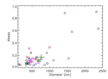
Understanding the size and albedo of 2013 FY27 is important in order to put this intrinsically bright object into context of the other dwarf planets beyond Neptune. The largest TNOs may have formed or evolved in a much different manner than the more moderate and smaller objects. The intrinsic brightness of 2013 FY27 means it is near the interesting transition regime between the largest few TNOs, which have high albedos and high densities, and the more moderate and smaller TNOs, which have moderate and lower albedos and densities (Brown 2013). There also seems to be some correlation between the color of a TNO and its albedo and dynamical classification (Lacerda et al. 2014). Most of the largest TNOs have known satellites, which one can use to find the bulk densities of the objects. The densities of the largest TNOs seem to be much higher ( ) than for the smaller TNOs ( ) (Brown 2013; Grundy et al. 2015; Barr & Schwamb 2016). This suggests the larger TNOs are made of more rock and less ice and have less porosity than the smaller TNOs. The intermediately sized large TNOs, like 2013 FY27, are thus key to understanding where, how and why this transition in albedo and density occurs. Through thermal and optical observations, we place 2013 FY27 into the context of the largest TNOs.
2 Magellan Optical Observations
We observed 2013 FY27 using the Magellan 6.5 meter telescope at Las Campanas, in Chile on UT March 8, 9 and 10 and May 3, 2016. The IMACS camera was used, which has a pixel scale of 0.20 arcsec per pixel and field of view of about 0.16 square deg. The geometry of the observations are shown in Table 1. All images were bias subtracted and flat fielded with nightly dithered sky twilight flats. Images were obtained guiding at sidereal rates in photometric conditions using the Sloan g, r or i-band filters.
Most of the Magellan images were obtained in the r-band to look for short-term variability of 2013 FY27 over minutes, hours and days. To determine the optical color of 2013 FY27, we observed 2013 FY27 multiple times on UT March 10, 2016 in the g-band and i-band Sloan filters as well as the r-band filter. The filters were rotated between the r, g and i-bands to prevent any possible short-term variations from effecting the color measurements and were obtained twice, separated by a few hours. We also convert the Sloan g,r,i colors to the Johnson-Morgan-Cousins BVRI filter system for easier comparison to some past works using the transformation equations from Smith et al. (2002): ; ; ; . Sheppard (2010) showed these transformations from g,r,i colors to BVRI colors are good to within a hundredth of a magnitude for most TNOs.
All the optical observations were calibrated using the Sloan standard star fields DLS1359-11 and PG1633+099. Seeing was between 0.6 and 1.5 arcseconds, with longer exposure times used when the seeing was worse. The photometry as well as the details of each individual image from the observations are shown in Table 2. All photometry was obtained similar to that described in Sheppard (2007) and used apertures to fit the variable seeing, ranging from 2.4 in the best seeing to 4 arcseconds in the worse seeing. The background counts for each image were subtracted off the photometry of the object using an aperture annulus that was larger than that used for the object’s photometry.
2.1 r-band Optical Light Curve
We observed 2013 FY27 in the r-band at Magellan over minutes, hours and days in early March 2016 to look for any short-term variations caused by rotation of the object. The observational results are shown in Table 2. No clear variability was seen, with variability being less than over the 3 days of observations from March 8 to March 10, 2016 (Figure 2). This suggests 2013 FY27 either has a very low amplitude rotational variability, or that its rotation is longer than a few days time. As 2013 FY27 is a large TNO, it should be mostly spherical in shape due to the strength of its own gravity. Any short-term variations would likely be from albedo differences on its surface, which we see no strong evidence for. There is also the less likely possibility that we are observing 2013 FY27 pole-on, and thus would see no rotational short-term variability.
2.2 Sloan Optical Colors
Using the Sloan , and -band observations from Magellan described above, we find the colors of 2013 FY27 are and giving mags (Table 3). Since the majority of TNOs have nearly linear color slopes at visible wavelengths, the basic color of a TNO can be reported as its spectral gradient (see Doressoundiram et al. 2008 and Sheppard 2010). The spectral gradient is the amount of reddening per 100 nanometers and can be found through
| (1) |
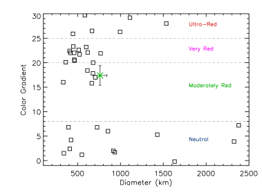
where and are the midpoint wavelengths for the filters used and and are the flux in the filters normalized to the V-band. We use the and filters to determine for 2013 FY27 as these filters have well separated central wavelengths. For 2013 FY27, we find the optical color spectral slope is . This color is moderately red when compared to other TNO colors taken from Hainaut et al. (2012) and the updated Minor Bodies in the Outer Solar System (MBOSS) data base (Figure 4).
It has been known since the first Kuiper Belt objects were discovered that they exhibit a very wide range of colors with possible color groupings (Luu & Jewitt 1996; Barucci et al. 2005). Ultra-red material is generally considered to have a large red spectral gradient of (Jewitt 2002; Sheppard 2010,2012). In Sheppard (2012) there is a noticeable gap in objects from the Cold Classical belt with colors just below , so we define as very red objects. Objects with spectral gradients between about 8 and 20 are considered moderately red while objects with color below this are considered neutral to blue in color.
It is apparent in Figure 4 that the ten largest TNOs only show extremes in colors, being either very neutral or ultra-red. It is not until objects smaller than about 800 km in diameter start to show very red and moderately red colors. This is interesting as the extreme colors are usually associated with organics and freshly exposed ices such as Methane, water ice and methanol (Brown et al. 2012; Dalle Ore et al. 2015; Fraser et al. 2015). This suggests the largest TNOs are continuing or have more recently modified their surfaces compared to the TNOs smaller than 800 km. Moderately red colors might be more expected on objects that have old surfaces as micrometeorite bombardment and irradiation would be expected to dull any exposed ices over time (Grundy 2009). The surfaces of the largest TNOs might be fresher because they can more easily hold on to volatile ices and could further have differentiated more completely and even have cryovolcanism occurring in recent times. 2013 FY27 is one of the largest known moderately red objects.
2.3 Optical Phase Curve
The optical apparent magnitude of a TNO depends on its radius (), distance from the Sun (), distance from Earth (), albedo () and phase angle (). The apparent optical magnitude can be calculated as,
| (2) |
where is the apparent magnitude of the Sun in the filter being used and the linear phase function can be represented as
| (3) |
where is the phase angle in degrees and is the linear phase coefficient in magnitudes per degree. At opposition, deg, and thus .
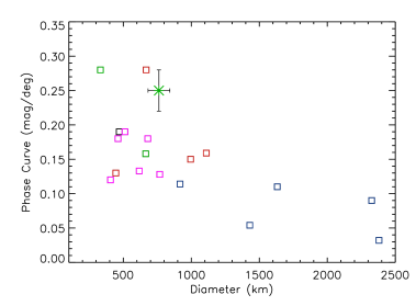
We further observed 2013 FY27 at Magellan on May 3, 2016 over several hours to determine its phase coefficient (Figure 3). Since no significant short-term light curve was found in March, any long-term variations in brightness are likely attributed to the different phase angles observed for 2013 FY27. The March 2016 observations were obtained at a phase angle near 0.18 degrees while the May observations had the object further from opposition, near 0.62 degrees (Table 1). Again, 2013 FY27 showed no significant variations over the nearly three hours of observations on May 3, 2016. The average r-band magnitude in March was mags and in May mags. 2013 FY27 should have been about 0.01 mags fainter in May because it was slightly further from the Earth at that time. Thus 2013 FY27 was about 0.11 mag fainter in May when accounting for differences in its distance from the Sun and Earth. We attribute the 0.11 mag difference from 2013 FY27 being 0.44 degrees further away from true opposition in May than the March observations.
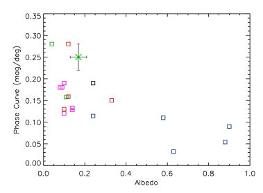
From the above March and May r-band observations, we find a phase coefficient of mags per deg for 2013 FY27. We show in Figure 5 the phase coefficients for the largest TNOs using data from Buie et al. (1997); Sheppard and Jewitt (2002),(2003); Rabinowitz et al. (2007); Sheppard (2007); Benecchi & Sheppard (2013). We confirm the finding in Sheppard (2007) that the largest few TNOs, which are all neutral in color with high albedos, show the lowest phase coefficients (Figure 6). The lower phase coefficient is likely from back scattering off a high albedo surface. 2013 FY27 has a higher than typical TNO phase coefficient, which are mostly in the 0.10 to 0.20 mag per degree range. This higher phase coefficient could signify different grain properties on 2013 FY27’s surface compared to the typical TNO or might be a sign of a very long and significant rotational light curve that would not be seen in a 3 day or less period of time.
For main belt asteroids, it appears the higher the phase coefficient, the lower the surface albedo (Belskaya and Shevchenko 2000). But main belt asteroids likely have different compositions and usually have lower phase coefficients than the TNOs. In addition, most asteroid phase curves are based over a much larger range of phase angles, in which the TNOs are not able to be viewed as they typically stay below about 2 degrees as seen from Earth. The opposition surge, when an object gets much brighter at very low phase angles from back-scattering effects, starts around 0.1 to 0.2 degrees (Belskaya et al. 2008). Thus the 2013 FY27 observations are just outside of the start of the opposition surge and likely not strongly affected by the opposition surge.
2.4 Optical Absolute Magnitude
Using the linear phase coefficient found above, we can calculate the reduced magnitude as
| (4) |
The reduced magnitude of a solar system object is the magnitude it would have if it were observed simultaneously at a geocentric and heliocentric distance of 1 au with a phase angle of 0 deg. Thus the reduced magnitude gives you the brightness of an object independent of observing geometry. The reduced magnitude brightness is for the most part only dependent on the size and albedo of an object.
Using the above equation, we find the reduced magnitude of 2013 FY27 at deg as mags in the r-band during the March 2016 observations. For the May 2016 observations, we find the reduced magnitude is mags at deg because the object is further from opposition and thus fainter from showing a less illuminated face towards Earth.
To calculate the reduced magnitude of 2013 FY27 when at zero degrees phase angle, we use the linear phase coefficient found above of mags per deg. So 2013 FY27 should be magsdeg deg mags brighter when at 0 deg phase angle compared to 0.18 deg phase angle assuming a linear phase function. Thus we find mags. From the transformation equations in Smith et al. (2002), we find the Johnson-Kron-Cousins R-band reduced magnitude is mags. Using the color found for 2013 FY27 of mags, we find mags, which we take as the absolute magnitude of 2013 FY27. This is slightly fainter than the current value used at the minor planet center for 2013 FY27, which is mags. This slight difference in the absolute magnitudes is to be expected as Sheppard (2007) found the Minor Planet Center is routinely off by several tenths of magnitudes from well measured calculated values of the absolute magnitude, likely because the Minor Planet Center uses all photometry from multiple sources and filters, some of which have low signal to noise and thus large uncertainties. Though the absolute magnitude generally uses a curved phase function as defined in Bowell et al. (1989), Sheppard (2007) found the reduced magnitude for TNOs using a linear phase function with is similar to within a few hundredths of the absolute magnitude phase function used in Bowell et al. (1989).
An important optical reference is to determine the optical brightness of 2013 FY27 at the time of the ALMA observations in late December 2017 and early January 2018. The phase angle and distance of 2013 FY27 at the time of the ALMA observations is very similar to the May 3, 2016 observations from Magellan. Thus we should be able to use the May 3, 2016 photometry as the base for the optical photometry during the ALMA observations. At this time , and mags, giving from color transformations using Smith et al. (2002) , and mags.
3 ALMA Observations
The Atacama Large Millimeter Array (ALMA) observations were taken on UT 29 and 30 December 2017 and 04 January 2018 in ALMA Cycle 5 under Project 2017.1.01662.S (Table 1). At that time, the array was configured with 46 antennas and a maximal distance between antennas (maximum baseline) of 2500 m. We used Band 3 in the standard continuum setup centered at 97.5 GHz, with a total encompassed bandwidth of 8 GHz. For such a cold object, Band 3 provides the best sensitivity in the continuum among all the ALMA bands making it the best to use as a first thermal detection attempt. The ALMA observations consisted of three sets of 66 minutes observations, one each on 29 and 30 December 2017 and another on 04 January 2018. The combined observations totaled of 3.3 hours of ALMA time, with 2.2 hours of that integrating on the source. The rest of the observation time was spent on quasars used as bandpass, flux and gain calibrators.
Interferometric measurements consist in visibilities, which are complex numbers corresponding to signal cross-correlations between each pair of antennas. For each of the observations, visibilities were calibrated using the ALMA calibration pipeline in the Common Astronomy Software Applications package (CASA, McMullin et al. 2007), to correct for the spectral response and temporal gain variations of the instrument. The absolute flux scale was assessed using the well monitored quasar J1127-1857 as a reference.
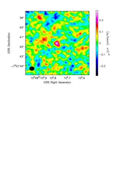
The three sets of observations were then combined, spectrally averaged and stacked into one visibility set. To obtain a continuum image, inverse Fourier transform and deconvolution were applied to the combined visibilities set. Since this experiment is a point-source detection which does not depend on spatial resolution, natural weighting was used to maximize sensitivity (at the expense of beam size), giving the final image an rms of 5.5 microJy. The synthesized beam was arcseconds in the natural-weighted image. 2013 FY27 was found very near the center of the image as expected, and was 25 microJy bright (Figure 7). This gives the ALMA detection of 2013 FY27 a Signal-to-Noise of about 4.5. To assess the quality of the flux calibration, we compared the results given by the calibration pipeline using J1127-1857 as a reference to the expected flux value for the phase calibrator J1058+0133, which is a relatively bright and well monitored quasar. The good match between the retrieved and expected flux for J1058+0133 allow us to determine that the absolute flux calibration is accurate at the 3 to 4 percent level.
4 Size and Albedo of 2013 FY27
To first order, the thermal flux from an object is proportional to , where is the effective diameter, is the geometric albedo in V-band, and is the phase integral. The reflected sunlight in the V-band from the same object is proportional to . As shown in Brown & Butler (2017), for TNOs can be approximated by . Thus we have two equations that can be solved for the two unknowns of diameter and albedo ( and ) (see e.g. Fernandez et al. 2013).
The most common method to determine the size and albedo of an object with single-epoch thermal photometry, as here with 2013 FY27, is to use the Near-Earth Asteroid Thermal Model (NEATM) of Harris (1998). Some basic assumptions used in NEATM are that (i) the object is spherical; (ii) the phase darkening of the thermal emission is entirely dependent on how much of the lit-up hemisphere of the object is facing Earth, and (iii) the basic dayside surface temperature falls off from the subsolar point as , where is the local zenith angle, and there is no thermal emission from the nightside.
These NEATM assumptions are reasonable for 2013 FY27. 2013 FY27 is probably close to spherical as it is likely large and there is little if any apparent shape-induced rotational modulation of our optical photometry (section 2.1). Our observations were obtained at very small phase angles and thus phase darkening uncertainties should be minimal. Regarding the temperature map, the NEATM is appropriate for a “slow rotator,” i.e. an object whose thermal inertia is sufficiently low, and rotation period sufficiently long, that the object has no thermal memory. In NEATM, deviation from a zero-thermal memory situation is encapsulated in the beaming parameter, , which will account for the cooler temperatures expected for an object with some thermal memory. A value of corresponds to the zero thermal memory situation, and a value of applies to cases with thermal memory, with the higher the value, the more memory (such as the case of a quick rotator or a large thermal inertia). For our analysis of 2013 FY27, since we have measurements at only one thermal wavelength, we cannot independently determine what the beaming parameter should be. However we can use other TNO measurements to examine what would be appropriate to assume. Lellouch et al. (2013, 2017), in a study of the thermal emission from several TNOs as observed with ALMA, Herschel, and Spitzer, found that the thermal inertias of these bodies are quite low, at least an order of magnitude below that of the Moon. It is likely safe to assume that 2013 FY27 is similar, and so should be close to acting like a slow rotator in the NEATM model for reasonable values of its rotation period. Lellouch et al. (2017) advise using a value of for TNOs observed with ALMA, so we adopt that value here. The other assumptions that go into NEATM are the emissivity and the visible-wavelength phase law. For the former, we assume a value of , as suggested by Lellouch et al. (2017). For the latter, we apply our results from section 2.3, where mag/deg.
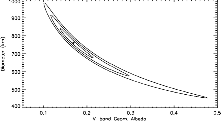
The results of our application of the NEATM to the 2013 FY27 photometry is shown in Figure 8. We used a flux density from thermal emission of Jy at a wavelength of 3.075 mm, and a V-band magnitude of to fit and . The thermal emission error bar incorporates the 4% uncertainty in the absolute calibration. Since there are zero degrees of freedom (using two measurements to fit two parameters), we cannot formerly calculate a reduced-; instead we use itself. The contour plot in Figure 8 shows contours of , 2, and 3, and we report an error bar on the best-fitting parameters to correspond to the level. We find that the best fit for 2013 FY27 is an effective diameter of km and . The two error bars are correlated, as the elongated contours show. The errors on and we report here are from the uncertainty in the photometry including the absolute calibration of the standard sources in both the visible and thermal. Incorporating the potential uncertainty in the assumed parameters such as the beaming parameter and effective slow rotation period is tricky, but could add some five percent uncertainty to the diameter calculation and 10 percent uncertainty to the albedo calculation. As noted in section 5 below, a satellite some 3 magnitudes fainter than 2013 FY27 was found in HST data. Assuming the satellite has a similar albedo as the primary, the satellite is about 190 km in diameter, making the primary slightly smaller than calculated above at km.
4.1 Discussion of Dwarf Planet Diameters, Albedos and Colors
An albedo of about 17% is on the high end for a moderately red object but consistent with the other moderately red and moderately sized dwarf planet TNOs (Figure 1). 2013 FY27 is one of the largest, if not the largest, moderately red TNO. All TNOs larger than 2013 FY27, of which there are about ten, have either ultra-red colors or neutral colors. The TNOs with similar sizes and smaller than 2013 FY27 (diameters km) start to show an abundance of moderately red or very red colors, unlike the largest ten objects, which do not show any of these middle surface colors and only the extreme surface colors.
This suggests something is or has physically changed the surfaces of the largest ten TNOs with diameters above 800 km compared to the TNOs with diameters smaller than 800 km. This could be because TNOs above about 800 km have enough self gravity to retain certain ices such as methane more readily on their surfaces than the smaller TNOs. Neutral colored surfaces are generally associated with fresh water ice while ultra-red surfaces are associated with organics and possibly other ices such as methanol and methane. The color differences may be because TNOs above 800 km retained enough internal heat to remain active longer or even to this day, to resurface their surfaces from possible cryovolcanism type events. TNOs above 800 km might also be more fully differentiated than TNOs below 800 km, making their two surfaces types different in composition. As TNOs below 800 km still show neutral and ultra-red surfaces as well as very red and moderately red surfaces, the moderately red surfaces might be a signature of a very old surface that has been bombarded by high energy photons, particles and micrometeorites over long periods of time, while the extreme colors are more of a sign of fresher surfaces from recent collisions or activity. Further analysis is required to determine why the largest TNOs do not show moderately red surfaces, but Figure 1 strongly suggests there is some kind of surface change around 800 km in diameter for TNOs.
5 Satellite Discovered around 2013 FY27
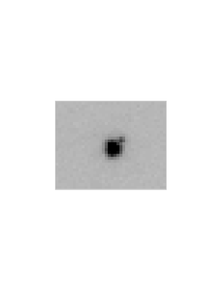
We observed 2013 FY27 with the Hubble Space Telescope (HST) on UT January 15, 2018 to look for possible satellites (HST Program GO-15248). Four 545 second images were taken with HST between 01:24 and 02:30 hours UT in the F350LP wide band filter (central wavelength of 5859 Angstroms) using the WFC3/UVIS instrument with a pixel scale of arcsec per pixel (MacKenty et al. 2014). An obvious point source was detected about arcseconds at a position angle of 135 degs from the primary (Figure 9). The satellite was seen in all four images and moved along with the motion of the primary, which was about -1.47 and 0.34 arcseconds an hour in Right Ascension and Declination, respectively. This detection was reported as a satellite of 2013 FY27 to the International Astronomical Union (see CBET 4537: Sheppard 2018). No satellite motion relative to the primary was detected between the first and last (fourth) image from HST, confirming its association with the primary and likely ruling out an extremely fast orbital period of a few days or less around the primary. The four HST images were aligned with respect to the primary and coadded to search for additional fainter satellites, but nothing obvious was detected to about 27.5 mags within a tenth to tens of arcseconds of the primary.
At the time of the HST observations, 2013 FY27 was 79.48 au from the Earth. Thus a 0.17 arcsecond separation means the satellite was at least 9800 km from the primary. The newly discovered satellite was mags fainter than the primary in the optical. Thus the diameter of the satellite, if assuming the same albedo as the primary, would be about 3.9 times smaller than the primary or about 190 km in diameter.
Additional HST observations of 2013 FY27 and its satellite have been obtained in May and July of 2018 under HST Program 15460. A full analysis of the new HST data will allow the determination of the satellites orbit and with the albedo reported in this work, a bulk density of the system can be determined giving insight into the composition and structure. The full detailed analysis using all of the HST observations for 2013 FY27 will be part of a future paper on the satellite and its orbit around 2013 FY27. We note that in Figure 7, there appears to be an extension of the ALMA signal to the southwest of the primary. This is unlikely to be the satellite of 2013 FY27 as we believe the satellite is nearly edge-on, and thus should only show up to the southeast and northwest of the primary. Obtaining the full orbit of the satellite will allow us to predict where it should have been during the ALMA observations and further analysis of the ALMA data and 2013 FY27’s satellite is left for the next paper on the full orbit of the 2013 FY27 system.
5.1 Discussion of Dwarf Planet Satellites
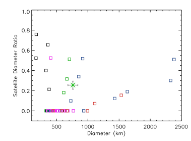
All of the largest known TNOs, those with diameters well over 1000 km, irrespective of their dynamical class, have known satellites (Pluto, Eris, Makemake, 2007 OR10, Haumea, and Quaoar) and now 11 of the top 15 largest TNOs have known satellites (Figure 10). All of the satellites of these largest objects are significantly smaller than the primary and have relatively close orbits that are indicative of collisional formation (Brown et al. 2006; Noll et al. 2008; Parker et al. 2016; Kiss et al. 2017; Brown & Butler 2018). This is remarkable that satellites seem to be the norm and not the exception for the largest objects. This appears to suggest the collisional formation of Earth’s moon and the satellites of Mars are normal outcomes of the planet formation process (Mercury and Venus likely have no satellites simply because their closeness to the massive Sun makes tidal interactions too strong for most satellite orbits around these planets to be stable over the age of the solar system).
Though we don’t know the full orbit of the satellite for 2013 FY27, its small size relative to the primary and relatively close distance suggest the satellite was likely created by a direct impact, similar to the scenarios envisioned for the other known satellites of the dwarf planets (Canup 2011; McKinnon et al. 2017). This formation scenario is quite different than the equal-sized, distant binaries found mostly in the main Kuiper Belt, which likely did not form through direct collisions onto the primary (Schlichting and Re’em 2008; Nesvorny et al. 2010; Parker et al. 2011; Sheppard et al. 2012).
Barr and Schwamb (2016) suggest that there are two possible collisional formation scenarios that could create the close-in satellites found around all the largest TNOs. High energy direct collisions could remove the ice from the primary, leaving a dense primary and small ice rich satellite. A glancing indirect collision would leave the primary volatile rich and thus of low density and could create larger satellites of similar composition to the primary. 2013 FY27 can be a further test to this theory through determining its density from knowing the full orbit of the satellite around the primary as well as looking at the surfaces of the primary and secondary for similarities or differences. We note in Figure 10 there appears to be a break in the ratio of the satellite size to the primary size for TNOs larger than about 900 km. TNOs larger than about 900 km have relatively small satellites compared to the primary (though Pluto somewhat breaks this trend). Many of the smaller TNOs appear to have satellites that are relatively large compared to the primary, with some approaching equal-sized binaries starting around 400 km in diameter.
6 Summary
2013 FY27 is intrinsically the brightest TNO not yet observed for its basic physical properties. 2013 FY27’s absolute magnitude of near 3 mags means it likely has a size that is near the transition region between the largest few TNOs that show high albedos and high densities and the smaller TNOs that show low to moderate albedos and densities. We observed 2013 FY27 over optical and thermal wavelengths at several telescopes to determine its physical characteristics for the first time and compare it to the other dwarf planets.
1) The geometric albedo of 2013 FY27 was found to be . The effective diameter of the 2013 FY27 system is km. Assuming then newly discovered satellite around 2013 FY27 has a similar albedo as the primary, the satellite is about 190 km in diameter, making the primary slightly smaller than the effective diameter of the system at km.
2) The color of 2013 FY27 was found to be moderately red with a spectral gradient of . This makes 2013 FY27 one of the largest known moderately red TNOs. All TNOs larger than about 800 km in size, of which there are about ten known, only show neutral or ultra-red surface colors. This could be because the largest several TNOs have different or fresher surfaces than TNOs smaller than 800 km from possible cryovolcanism, differentiation and/or abundant exposed surface ices. The TNOs only start to show moderately red colors for objects less than about 800 km in diameter, and they appear to be very abundant below this threshold. As there is also neutral and ultra-red TNOs below 800 km, it suggests the moderately red color might be an indication of an old surface while the more neutral and ultra-red colors in the smaller TNOs could be fresh surfaces exposed from recent impacts or other processes.
3) A satellite of 2013 FY27 was found in Hubble Space Telescope observations of 2013 FY27. It is some mags fainter and was arcsec away from the primary at discovery. The satellite diameter to primary diameter ratio is a little larger than most of the ratios found for the largest TNOs. There appears to be a difference in the satellite to primary size ratios starting around the TNOs over about 900 km. Less than 900 km the satellite to size ratio increases until near 400 km in primary size one starts to approach equal-sized binaries. For TNOs larger than 900 km, the satellite to primary size ratio is generally smaller, with Pluto being an exception.
4) 2013 FY27 was monitored over minutes, hours and days with no obvious short-term variability detected in the r-band. The most likely reason for no measureable short-term light curve is that 2013 FY27 is near spherical in shape with no significant albedo variations on its surface to allow for a measurable rotational period. 2013 FY27 was further monitored in the r-band over months to find its linear phase curve of mags/deg. This is a slightly higher than normal TNO phase curves, but reasonable for a moderate albedo surface, unlike the lower phase curves found for very high albedo TNO surfaces. The reduced magnitude of 2013 FY27 was found to be and mags.
Acknowledgments
We thank D. Ragozzine for comments on the manuscript and sharing the initial analysis of the 2013 FY27 satellite orbit. This paper makes use of the following ALMA data: ADS/JAO.ALMA#2017.1.01662.S. ALMA is a partnership of ESO (representing its member states), NSF (USA) and NINS (Japan), together with NRC (Canada), NSC and ASIAA (Taiwan), and KASI (Republic of Korea), in cooperation with the Republic of Chile. The Joint ALMA Observatory is operated by ESO, AUI/NRAO and NAOJ. The National Radio Astronomy Observatory is a facility of the National Science Foundation operated under cooperative agreement by Associated Universities, Inc. This work is based in part on NASA/ESA Hubble Space Telescope Cycle 25 Program 15248 observations. This paper includes data gathered with the 6.5 meter Magellan Telescopes located at Las Campanas Observatory, Chile.
References
- (1)
- (2) Barucci, M., Belskaya, I., Fulchignoni, M. & Birlan, M. 2005, AJ, 130, 1291.
- (3)
- (4) Barr, A. & Schwamb, M. 2016, MNRAS, 460, 1542.
- (5)
- (6) Belskaya, I. & Shevchenko, V. 2000, Icarus, 147, 94.
- (7)
- (8) Belskaya, I., Levasseur-Regourd, A., Shkuratov, Y. & Muinonen, K. 2008, in The Solar System Beyond Neptune, ed. M. Barucci, H. Boehnhardt, D. Cruikshank and A. Morbidelli (Tucson: Univ of Arizona Press), 115-127.
- (9)
- (10) Benecchi, S. & Sheppard, S. 2013, AJ, 145, 124.
- (11)
- (12) Brown, M., van Dam, M., Bouchez, A., et al. 2006, ApJ, 639, 43.
- (13)
- (14) Brown, M., Schaller, E. & Fraser, W. 2012, AJ, 143, 146.
- (15)
- (16) Brown, M. 2013, ApJ, 778, L34.
- (17)
- (18) Brown, M. & Butler, B. 2017, AJ, 154, 19.
- (19)
- (20) Brown, M. & Butler, B. 2018, arXiv:1801.07221.
- (21)
- (22) Buie, M., Tholen, D. & Wasserman, L. 1997, Icarus, 125, 233.
- (23)
- (24) Canup, R., 2011, ApJ, 141, 35.
- (25)
- (26) Dalle Ore, C., Barucci, M., Emery, J. et al. 2015, Icarus, 252, 311.
- (27)
- (28) Doressoundiram, A., Boehnhardt, H., Tegler, S. and Trujillo, C. 2008, in The Solar System Beyond Neptune, ed. M. Barucci, H. Boehnhardt, D. Cruikshank and A. Morbidelli (Tucson: Univ of Arizona Press), 91-104.
- (29)
- (30) Fernandez, Y., Kelley, M., Lamy, P., et al. 2013, Icarus, 226, 1138.
- (31)
- (32) Ferrari, C. & Lucas, A. 2016, A&A, 588, 133.
- (33)
- (34) Fraser, W., Brown, M. & Glass, F. 2015, ApJ, 804, 31.
- (35)
- (36) Gerdes, D., Sako, M., Hamilton, S., et al. 2017, ApJ, 839, L15.
- (37)
- (38) Grundy, W. 2009, Icarus, 199, 560.
- (39)
- (40) Grundy, W., Porter, S., Benecchi, S. et al. 2015, Icarus, 257, 130.
- (41)
- (42) Harris, A. 1998, Icarus, 131, 291.
- (43)
- (44) Hainaut, O., Boehnhardt, H. & Protopapa, S. 2012, A&A, 546, 115.
- (45)
- (46) Jewitt, D. 2002, AJ, 123, 1039.
- (47)
- (48) Kiss, C., Marton, G., Farkas-Takacs, A. et al. 2017, ApJ, 838, 1.
- (49)
- (50) Kovalenko, I., Doressoundiram, A., Lellouch, E., Vilenius, E., Muller, T. & Stansberry, J. 2017, A&A, 608, 19.
- (51)
- (52) Lacerda, P., Fornasier, S., Lellouch, E., et al. 2014, ApJ, 793, L2.
- (53)
- (54) Lebofski et al. 1989, Icarus, 78, 335
- (55)
- (56) Lellouch, E., Santos-Sanz, P., Lacerda, P. et al. 2013, A&A, 557, A60.
- (57)
- (58) Lellouch, E., Moreno, R., Muller, T., et al. 2017, A&A, 608, 45.
- (59)
- (60) McMullin, J. P., Waters, B., Schiebel, D., Young, W., & Golap, K. 2007, Astronomical Data Analysis Software and Systems XVI (ASP Conf. Ser. 376), ed. R. A. Shaw, F. Hill, & D. J. Bell, 127.
- (61)
- (62) MacKenty, J., Baggett, S., Brammer, G., Hilbert, B., Long, K., McCullough, P. & Adam, G. 2014, Proc. SPIE, 9143, 914328.
- (63)
- (64) McKinnon, W., Stern, S., Weaver, H., et al. 2017, Icarus, 287, 2.
- (65)
- (66) Nesvorny, D., Youdin, A., & Richardson, D. 2010, AJ, 140, 785.
- (67)
- (68) Noll, K., Grundy, W., Chiang, E., Margot, J. & Kern, S. 2008, in The Solar System Beyond Neptune, ed. M. Barucci, H. Boehnhardt, D. Cruikshank and A. Morbidelli (Tucson: Univ of Arizona Press), 345-363.
- (69)
- (70) Parker, A., Kavelaars, J., Petit, J., Jones, L., Gladman, B. & Parker, J. 2011, ApJ, 743, 1.
- (71)
- (72) Parker, A., Buie, M., Grundy, W., & Noll, K. 2016, ApJ, 825, 9.
- (73)
- (74) Rabinowitz, D., Schaefer, B. & Tourtellotte, S. 2007, AJ, 133, 26.
- (75)
- (76) Santos-Sanz, P., Lellouch, E., Groussin, O., Lacerda, P., Muller, T., Ortiz, J., Kiss, C., Vilenius, E., Stansberry, J., Duffard, R., Fornasier, S., Jorda, L. & Thirouin, A. 2017, A&A, 604, 95.
- (77)
- (78) Schlichting, H. & Re’em, S. 2008, ApJ, 673, 1218.
- (79)
- (80) Sheppard, S. & Jewitt, D. 2002, AJ, 124, 1757.
- (81)
- (82) Sheppard, S. & Jewitt, D. 2003, EM&P, 92, 207.
- (83)
- (84) Sheppard, S. 2007, AJ, 134, 787.
- (85)
- (86) Sheppard, S. 2010, AJ, 139, 1394.
- (87)
- (88) Sheppard, S. 2012, AJ, 144, 169.
- (89)
- (90) Sheppard, S., Ragozzine, D., & Trujillo, C. 2012, AJ, 143, 58.
- (91)
- (92) Sheppard, S. & Trujillo, C. 2016, AJ, 152, 221.
- (93)
- (94) Sheppard, S. 2018, CBET, 4537.
- (95)
- (96) Smith, J., Tucker, D., Kent, S., et al. 2002, AJ, 123, 2121.
- (97)
- (98) Stansberry, J., Grundy, W., Brown, M., Cruikshank, D., Spencer, J., Trilling, D. and Margot, J. 2008, in The Solar System Beyond Neptune, ed. M. Barucci, H. Boehnhardt, D. Cruikshank and A. Morbidelli (Tucson: Univ of Arizona Press), 161-179.
- (99)
| Name | UT Date | Telescope | |||
|---|---|---|---|---|---|
| (AU) | (AU) | (deg) | |||
| 2013 FY27 | 2016 Mar 08 | 80.26 | 79.30 | 0.17 | Magellan |
| 2013 FY27 | 2016 Mar 09 | 80.26 | 79.30 | 0.18 | Magellan |
| 2013 FY27 | 2016 Mar 10 | 80.26 | 79.30 | 0.18 | Magellan |
| 2013 FY27 | 2016 May 03 | 80.24 | 79.73 | 0.62 | Magellan |
| 2013 FY27 | 2017 Dec 29 | 80.09 | 79.74 | 0.66 | ALMA |
| 2013 FY27 | 2017 Dec 30 | 80.09 | 79.72 | 0.66 | ALMA |
| 2013 FY27 | 2018 Jan 04 | 80.09 | 79.64 | 0.63 | ALMA |
| 2013 FY27 | 2018 Jan 15 | 80.08 | 79.48 | 0.56 | HST |
| UT DateaaUniversal date at the start of the integration. | Airmass | ExpbbExposure time for the image. | Mag.ccApparent red magnitude (r-band), uncertainties are to . |
|---|---|---|---|
| yyyy mm dd hh:mm:ss | (sec) | () | |
| 2016 03 08 01:43:32 | 1.36 | 225 | 21.91 |
| 2016 03 08 01:48:45 | 1.34 | 225 | 22.00 |
| 2016 03 08 02:20:38 | 1.23 | 225 | 21.96 |
| 2016 03 08 02:25:53 | 1.21 | 225 | 21.99 |
| 2016 03 08 02:56:24 | 1.15 | 225 | 21.95 |
| 2016 03 08 03:25:11 | 1.10 | 300 | 21.94 |
| 2016 03 08 04:00:14 | 1.08 | 250 | 21.91 |
| 2016 03 08 04:46:55 | 1.08 | 250 | 21.89 |
| 2016 03 08 05:36:42 | 1.13 | 300 | 21.95 |
| 2016 03 08 07:14:42 | 1.45 | 350 | 21.95 |
| 2016 03 08 07:35:49 | 1.58 | 350 | 21.95 |
| 2016 03 09 00:30:34 | 1.86 | 400 | 21.95 |
| 2016 03 09 00:39:18 | 1.77 | 400 | 21.98 |
| 2016 03 09 01:15:27 | 1.49 | 400 | 21.99 |
| 2016 03 09 01:23:45 | 1.44 | 380 | 21.98 |
| 2016 03 09 01:31:36 | 1.40 | 380 | 21.92 |
| 2016 03 09 01:54:21 | 1.30 | 400 | 21.92 |
| 2016 03 09 02:02:28 | 1.27 | 400 | 21.92 |
| 2016 03 09 02:24:01 | 1.21 | 380 | 21.92 |
| 2016 03 09 02:31:47 | 1.19 | 400 | 21.96 |
| 2016 03 09 03:04:00 | 1.13 | 400 | 21.94 |
| 2016 03 09 03:12:11 | 1.12 | 350 | 21.96 |
| 2016 03 09 04:11:13 | 1.07 | 330 | 21.92 |
| 2016 03 09 04:55:11 | 1.09 | 350 | 21.93 |
| 2016 03 09 05:54:18 | 1.17 | 350 | 21.93 |
| 2016 03 09 07:21:05 | 1.51 | 330 | 21.94 |
| 2016 03 09 07:38:33 | 1.63 | 280 | 21.98 |
| 2016 03 10 01:01:19 | 1.55 | 330 | 21.93 |
| 2016 03 10 01:31:04 | 1.38 | 330 | 21.93 |
| 2016 03 10 02:19:26 | 1.21 | 300 | 21.92 |
| 2016 03 10 02:48:42 | 1.15 | 250 | 21.89 |
| 2016 03 10 03:31:37 | 1.09 | 275 | 21.92 |
| 2016 03 10 05:08:40 | 1.11 | 220 | 21.90 |
| 2016 03 10 06:31:05 | 1.29 | 280 | 21.90 |
| 2016 03 10 07:38:46 | 1.67 | 250 | 21.94 |
| 2016 05 02 23:28:15 | 1.13 | 300 | 22.06 |
| 2016 05 02 23:33:56 | 1.12 | 250 | 22.04 |
| 2016 05 03 00:47:00 | 1.08 | 200 | 22.03 |
| 2016 05 03 02:14:34 | 1.17 | 250 | 22.06 |
| Qtty | Measurement |
|---|---|
| H | mag |
| mags | |
| mags | |
| mags | |
| deg) | mag |
| deg) | mag |
| mag | |
| mag | |
| mag | |
| deg) | mag |
| deg) | mag |
| V-R | mag |
| R-I | mag |
| Effective Diameter | km |
| Primary Diameter | km |
| Satellite Diameter | km |
Note. — H is the absolute magnitude in the V-band. The colors are from the Sloan g, r and i-bands and have also been converted to the Johnson-Kron-Cousins system B, V, R and I-bands using Smith et al. (2002). is the spectral gradient of the object as described in Sheppard (2010).