Astrophysical Validation
Abstract
We present examples of validating components of an astrophysical simulation code. Problems of stellar astrophysics are multi-dimensional and involve physics acting on large ranges of length and time scales that are impossible to include in macroscopic models on present computational resources. Simulating these events thus necessitates the development of sub-grid-scale models and the capability to post-process simulations with higher-fidelity methods. We present an overview of the problem of validating astrophysical models and simulations illustrated with two examples. First, we present a study aimed at validating hydrodynamics with high energy density laboratory experiments probing shocks and fluid instabilities. Second, we present an effort at validating code modules for use in both macroscopic simulations of astrophysical events and for post processing Lagrangian tracer particles to calculate detailed abundances from thermonuclear reactions occurring during an event.
1 Introduction
Verification and validation (V&V) of models and simulations of astrophysical phenomena present challenges because the problem of studying these phenomena is largely one of indirectly observing multi-scale, multi-physics events. Other aspects of astrophysics also contribute challenges. The enormous length scales of astrophysical objects and vast distances to most astrophysical events preclude ready experimental access, limiting the availability of validation data. As with a great many applications, models suffer from epistemic uncertainty in the underlying basic physics (e.g. turbulence, fluid instabilities, and nuclear reaction rates), which is difficult to control and assess in simulations incorporating multiple interacting physical processes. The large range of length and time scales in many astrophysical problems frequently necessitates capturing sub-grid-scale physics within simulations, relevant examples being thermonuclear flames and turbulent combustion. The requirement of the development of sub-grid-scale models for these physical processes obviously introduces an additional level of complexity to V&V. Finally, the magnitude of the requisite computations for astrophysical events means that even with sub-grid-scale models, simulations may only capture the bulk effect of the underlying physics and some properties such as detailed compositions must be obtained by post-processing the simulation results with augmenting, higher-fidelity routines.
Even with these issues, V&V are vital parts of computational astrophysics as with any research domain. We present two studies aimed at validating components of Flash, a freely available, parallel, adaptive mesh simulation code used for modeling astrophysical phenomena and other applications. We first present a study of validating the hydrodynamics routines in Flash with experiments designed to replicate the high energy density environments of astrophysics and probe the underlying physics. The investigation formally addresses the issues of concern in validating hydrodynamics and serves as a well-controlled case study. The second study we present addresses physics that is difficult to include in whole-star simulations, due to limits in computing power, but that can be incorporated with approximate models and also calculated by post-processing simulation results. The problem is thermonuclear combustion and describing the overall reactions while including minimal nuclear species, and this work addresses the issue of comparing prohibitively expensive detailed models and simpler models that allow three-dimensional simulations.
As we will describe below, the challenges to astrophysical validation made parts of our study incomplete. The effort, however, was rewarding and very much worth the investment. Verification tests quantified the accuracy of code modules for problems with an analytic or accepted result, and the regular application of these tests serves for regression testing as the code is developed. Validation tests, though incomplete, demonstrated reasonable agreement between experiment and simulation for the case of the hydrodynamics study. Comparison between models of increasing sophistication allowed us to quantify the trade-off between fidelity of the method and expense. These studies all led to a deeper understanding of the underlying physics, and while we cannot say the modules and code were completely “validated,” the process greatly increased our confidence in the results.
2 Approach to Verification and Validation
Our methods for V&V largely follow accepted practices from the fluid dynamics community (AIAA, 1998; Roache, 1998a, b; Oberkampf and Roy, 2010, see Ch. 26 by Roache in this volume). We adopt the following definitions (based on definitions from the American Institute of Aeronautics and Astronautics (AIAA, 1998)).
Model: A representation of a physical system or process intended to enhance our ability to understand, predict, or control its behavior.
Simulation: The exercise or use of a model. (That is, a model is used in a simulation).
Verification: The process of determining that a model implementation accurately represents the developer’s conceptual description of the model and the solution of the model.
Validation: The process of determining the degree to which a model is an accurate representation of the real world from the perspective of the intended uses of the model.
Uncertainty: A potential deficiency in any phase or activity of the modeling process that is due either to a lack of knowledge (epistemic uncertainty or incertitude) or due to variability or inherent randomness (aleatory uncertainty).
Error: A recognizable deficiency in any phase or activity of modeling that is not due to lack of knowledge.
Prediction: Use of a model to foretell the state of a physical system under conditions for which the model has not been validated.
Calibration: The process of adjusting numerical or physical modeling parameters in the computational model for the purpose of improving agreement with experimental data.
Our definition of uncertainty differs from the original definition of the AIAA in that we expand the definition of uncertainty to also include aleatory uncertainty (see Calder et al, 2018; Hoffman et al, 2018, and references therein).
Another perspective comes from Roache (1998b), who offers a concise, albeit informal, summary of V&V terminology:
First and foremost, we must repeat the essential distinction between Code Verification and Validation. Following Boehm (1981) and Blottner (1990), we adopt the succinct description of “Verification” as “solving the equations right”, and “Validation” as “solving the right equations”. The code author defines precisely what partial differential equations are being solved, and convincingly demonstrates that they are solved correctly, i.e. usually with some order of accuracy, and always consistently, so that as some measure of discretization (e.g. the mesh increments) , the code produces a solution to the continuum equations; this is Verification. Whether or not those equations and that solution bear any relation to a physical problem of interest to the code user is the subject of Validation.
Roache also notes that a “code” cannot be validated, but only a calculation or range of calculations can be validated. Roache also makes a distinction between verifying a code and verifying a calculation, noting that “use of a verified code is not enough.” We also adhere to this explication of V&V terminology and note that following Roache, validation can be described as probing the range of validity of a code or model (Calder et al, 2002).
Our approach to verification consists of testing simulation results against analytic or benchmarked solutions and quantifying the error. The comparisons typically consist of simulations performed at increasing spatial and/or temporal resolutions to confirm convergence of the simulation to the correct answer. Details of these tests have appeared in the literature, and many of the tests are incorporated into automated regression testing of Flash (Calder et al, 2002; Weirs et al, 2005, 2005; Dwarkadas et al, 2005; Hearn et al, 2007; Dubey et al, 2009, 2015).
We validate by performing similar tests against data from experiments designed to replicate astrophysical environments. We take a hierarchical approach to validation, beginning by isolating the basic underlying physics and testing how well simulations capture it. We then devise tests of aggregate problems that capture the expected behavior of the astrophysical events. In the case of sub-grid models or post-processed results, we simulate simple problems with these models and compare against either actual validation data or direct numerical simulations. As with verification, we perform convergence tests, though as we describe below the process of demonstrating convergence is difficult for some fluid dynamics problems.
Another aspect of our testing concerns quantifying error on the adaptive simulation mesh (described below). Our approach is to test solutions on the finest simulation mesh against data or a solution, but the methodology for quantitatively comparing the solution at the different resolutions of an adaptive mesh is incomplete (Li, 2010; van der Holst et al, 2011; Shu et al, 2017; Li and Wood, 2017). We typically check for consistency between simulations on an adaptive mesh and simulations of the same problem on a fully-refined mesh while quantifying the accuracy of the solution on the fully-refined mesh (Calder et al, 2002). Also, in addition to problems characterizing solutions on an adaptive mesh, just simulating fluids at the extreme Reynolds numbers of astrophysics on adaptive meshes presents challenges (Kritsuk et al, 2006; Mitran, 2009). We describe the difficulties of simulating extreme Reynolds number flow in the discussion of our hydrodynamics method below.
We close discussion of our approach to V&V with a general note on the role of validation in astrophysics. Because of the literally astronomical distances to astrophysical events and extreme conditions involved, experimentally accessing astrophysical phenomena or even just replicating the environments of astrophysics is difficult. Thus one cannot readily perform validation experiments, which typically leads to an incomplete process of validation. Simulations of astrophysical events are therefore generally in the realm of prediction, that is, foretelling the state of a physical system under conditions for which the model has not been validated. Despite this, the process of V&V in astrophysics serves to build confidence in these predictions even if one cannot conclude that simulations or codes are “validated.”
3 Simulation Instruments
Our principal simulation instrument is the Flash code, which we use for simulating astrophysical events. Fundamentally, Flash simulates problems of fluid dynamics and consists of solvers for hydrodynamics and the additional physics of astrophysical events (described below). With Flash, we construct the numerical implementation of our conceptual model of the astrophysical event, and the act of simulating is the exercise of the model. We note that the exercise of a model is far more than just solving a set of differential equations. Multi-physics applications like astrophysics combine multiple solvers, each of which may rely on possibly uncontrolled assumptions (See Winsberg, 2010, for a thorough discussion). For this reason, we take the hierarchical approach to validation of modules in Flash mentioned above.
Our second instrument is a nucleosynthetic post-processing toolkit used in tandem with Flash. In the case of supernovae, comparison to observations requires the calculation of light curves (the intensity of light from the object as a function of time) and spectra. However, the yield of a particular element, titanium for example, may be critical for accurate spectra, but mostly unimportant to the energy release. Many elements fall into this category, so that the computation of the explosion is much less expensive when split into two stages. The energy release and explosion is computed with a small number of species in Flash, and is followed by post-processing to obtain all important species. The post-processing tools we present below apply state-of-the-art nuclear reaction networks to Lagrangian thermodynamic histories sampled from the Flash simulation. The resulting abundances are used to calculate light curves and spectra (e.g. Miles et al, 2016).
3.1 The Flash Code
The simulation instrument we use for modeling astrophysics events is the Flash code, developed at the University of Chicago (Fryxell et al, 2000; Calder et al, 2000; Dubey et al, 2009, 2013, 2014). Flash is a parallel, adaptive-mesh, hydrodynamics plus additional physics code originally designed for the compressible fluid flows associated with astrophysics. Flash incorporates multiple hydrodynamics methods (Fryxell et al, 2000; Lee and Deane, 2009; Lee, 2013; Lee et al, 2017a, b) coupled with modules for the requisite additional physics of the applications. In particular, Flash has undergone considerable development for high energy density physics applications (Tzeferacos et al, 2015).
The hydrodynamics modules solve the Euler equations of compressible hydrodynamics, shown here with gravitational sources as would apply to a self-gravitating problem such as a star.
Here is the mass density, is the velocity, is the pressure, is the internal energy of the gas, is the gravitational acceleration, and represents any additional source. The system is closed by an equation of state of the form
and Flash offers choices for particular applications. Flash calculates the acceleration due to gravity from the gravitational potential,
which is calculated by solving the Poisson equation for self-gravity
Here is the gravitational potential and is Newton’s gravitational constant. Flash also tracks different material species by advecting mass scalars,
where is the mass fraction of a given species (Fryxell et al, 2000).
Our first validation example addressed the Flash hydrodynamics module (without gravity) for the case of experiments involving fluid instabilities thought to occur during one class of stellar explosions known as a core collapse supernova (Fryxell et al, 1991). The particular hydrodynamic module in Flash used for this study is based on the PROMETHEUS code (Fryxell et al, 1989) and evolves the Euler equations in one, two, or three dimensions using a modified version of the Piecewise-Parabolic Method (PPM) (Colella and Woodward, 1984). The implementation allows use of general equations of state as is required for simulating stellar material (Colella and Glaz, 1985), but this capability was not used in the validation example.
PPM is a higher-order version of the method developed by Godunov (Godunov, 1959; Godunov et al, 1962), a finite-volume conservation scheme that solves the Riemann problem at the interfaces of the control volumes to compute fluxes into each volume. The conserved fluid quantities are treated as cell averages that are updated by the fluxes at the interfaces. This treatment has the effect of introducing explicit non-linearity into the difference equations and permits the calculation of sharp shock fronts and contact discontinuities without introducing significant non-physical oscillations into the flow. In addition, PPM utilizes a dissipative shock capturing scheme to further stabilize shocks and contact discontinuities, and is thus not directly solving the Euler equations (Majda, 1984; Winsberg, 2010).
The adaptive mesh of Flash is block structured and is supported primarily through the Paramesh Library (MacNeice et al, 1999, 2000), though it is under the process of migrating to the AMReX library (AMReX, 2018). The view of AMReX from other units in the Flash code will remain similar to that of Paramesh, and in the near future the two packages will be available as alternative implementations of the Grid unit. Later, the support for Paramesh may be dropped if it becomes too inefficient on newer platforms.
3.2 The Post-processing Toolkit
The nucleosynthetic post-processing toolkit uses the recorded Lagrangian history of fluid elements to compute the yield of nuclides (elements and their isotopes) produced in a stellar explosion (Travaglio et al, 2004; Townsley et al, 2016). The Lagrangian thermodynamic history is determined by integrating the position of a conceptual microscopic fluid element by
where is the initial position and is the velocity field as computed by the hydrodynamic simulation. This conceptual fluid element is often called a particle because it moves as a fluid-embedded particle would. From the resulting , it is possible to also record the thermodynamic state, namely and , the temperature and density, respectively. Such recorded histories are often called tracks or trajectories because they represent how the fluid element evolves in location and thermodynamic state space as a function of time.
Nucleosynthetic post-processing is performed in order to obtain the composition of material after it is processed by combustion and ejected. Composition is parameterized by abundances of various species quantified as the fraction of a unit of mass that is in the form of a particular species. For example, the fraction, by mass, that is in the form of 12C, may be written , and must be between 0 and 1. The abundances are found in post-processing by integrating
where are determined by the density and temperature-dependent reaction rates for processes which involve species . Any given specie is typically involved in multiple reactions, forming a network that is used to evaluate each rate. The end of the necessary integrations is typically well defined. As the star expands and fall until most reactions will become very slow compared to the time being simulated, effectively freezing out. Consideration of further evolution, typically radioactive decay, may be necessary depending on the usage of the resulting abundances. These integrations are typically performed for a large number of tracks which sample the ejected material by a suitably distributed choice of their initial positions .
3.3 Simulating Reactive Flow
With both Flash and the post-processing toolkit, the goal of simulations is to capture the evolution of stellar material during the course of an astrophysical event. Because stars are essentially self-gravitating gas, the interiors of stars are well described by the equations of fluid flow. During an astrophysical event, thermonuclear reactions drive the evolution by changing the composition and by releasing energy, which changes thermodynamic conditions like pressure and density. This combustion typically occurs in a relatively small region of space, e.g. a thin flame, that may be difficult to resolve in simulations of the event. The two validation examples we present address the two principal parts- fluid flow, including shocks and fluid instabilities, and the evolution of the composition.
For fluid dynamics problems, there are two fundamental classes of simulation distinguished by whether or not the scales of the numerical grid can resolve viscous effects (Calder et al, 2002; Winsberg, 2010, and references therein). Simulations that can resolve viscous effects are said to be “Direct Numerical Simulations,” while those that cannot and rely on a (possibly uncontrolled) sub-grid-scale model for viscous effects are referred to as “Large Eddy Simulations.” An eddy is a fluid current whose flow direction differs from that of the general flow, and the motion of the fluid is the net result of the movements of the eddies that compose it (Encyclopaedia Britannica, 2006). Large eddy simulations do not resolve either the explicit viscosity of the fluid or the contribution to the viscosity from eddies on unresolved scales (Fureby, 1996; Zhiyin, 2015, and references therein).
The issue of convergence of a solution for fluid flows is not as simple as it might seem. The enormous size of objects means that astrophysical regimes typically have Reynolds numbers far in excess of the Reynolds numbers of terrestrial flows, which are themselves higher than can be readily captured in hydrodynamics simulations. Even when run on contemporary supercomputers, simulations cannot capture the possibly Reynolds numbers of astrophysical flows making direct numerical simulations impossible. Thus simulations of astrophysical events are large eddy simulations that can either rely on sub-grid-scale models for turbulent flow or just allow the intrinsic numerical diffusion of the hydrodynamics method to set the limiting Reynolds number. This latter case, know as Implicit Large Eddy Simulation (ILES), is frequently applied and is the approach taken in the studies presented here. In ILES, changing the resolution changes the effective viscosity and hence the Reynolds number, which changes the problem itself and leads to the question of convergence of results with resolution. Considerable study has gone into determining the validity of this approach (Margolin and Rider, 2002; Grinstein et al, 2007; Margolin and Shashkov, 2008; Margolin, 2014). As our results show, large eddy simulations may not demonstrate convergence of a solution with resolution.
4 Validation Examples
As of this writing, Flash has had 20 years of development by generations of scientists. Much of this effort has been subjected to rigorous V&V (Calder et al, 2002; Timmes et al, 2004; Weirs et al, 2005, 2005; Dwarkadas et al, 2005; Hearn et al, 2007; Dubey et al, 2009, 2015; Townsley et al, 2016). In this contribution, we present two examples of validating the Flash code and post-processing toolkit for astrophysical applications. The first example is from early work comparing simulations to laboratory experiments addressing fluid instabilities in high energy density environments similar to the interiors of stars. The second example is ongoing work on computing reaction products in three-dimensional simulations of type Ia supernovae. This study includes comparison between methods for use in the simulations of the events and for calculating detailed abundances from the density and temperature histories of Lagrangian tracers.
While this contribution describes two examples of the V&V efforts for the Flash code, we note that V&V efforts continue as the capabilities and applications of Flash evolve. A recent survey of software engineering practice in scientific computing includes Flash as a case study and offers an independent perspective on the development of Flash (Storer, 2017).
4.1 Overview of Flash Problems
The Flash code was originally designed to investigate astrophysical thermonuclear flashes, explosive events powered by thermonuclear fusion. These events all involve a close binary star system with matter being transferred (accreted) onto a compact star (either a white dwarf or a neutron star) from a companion (Rosner et al, 2000). The three flash problems originally addressed by Flash were type I x-ray bursts (Zingale et al, 2001), classical novae (Alexakis et al, 2004), and type Ia supernovae (Plewa et al, 2004; Townsley et al, 2007).
X-ray bursts occur when a thermonuclear runaway occurs in a thin m layer of H- or He-rich fuel accreted onto the surface of a neutron star. The radius of the underlying neutron star my be inferred from observations and thereby allow constraints on the properties of dense matter. Classical novae occur when a thermonuclear m thick layer of H-rich material similarly explodes. In this case, material from the explosion is unbound and these events are thought to synthesize some intermediate-mass elements found in the galaxy. Type Ia supernovae are thought to occur when a pair of white dwarf star merge and/or when a white dwarf accretes enough mass to ignite fusion in the core. In this case, enough energy is added to overcome the gravitational binding and the star is completely disrupted, producing a bright explosion that may be used as an indicator for cosmological distances. (See references in above works for literature on each astrophysical topic, and Calder et al 2013 for an overview of ongoing investigation of Type Ia Supernovae.)
As mentioned above, these problems involve reactive flow, and in all cases there is a vast difference between the length scale of the combustion front and the astrophysical object. Hence the need for sub-grid-scale models. Fluid instabilities that may influence the burning rate are also of particular importance (Calder et al, 2007; Zhang et al, 2007; Townsley et al, 2016). Accordingly, the validation examples we present address problems of combustion and fluid instabilities.
4.2 Shocks and Fluid Instabilities
The high energy density environments of intense lasers interacting with matter are similar to the interiors of stars, and experiments offer opportunities for a quantitative comparison between data and simulation not possible with observations of astrophysical phenomena. The validation study we present was performed by a collaboration between Flash developers and experimentalists working at the Omega laser at the University of Rochester (Soures et al, 1996; Boehly et al, 1995; Bradley et al, 1998). The experiment chosen for the study involved a shock propagating through a multi-layer target with layers of decreasing density and was designed to produce hydrodynamic instabilities thought to arise during an astrophysical event known as a core collapse supernova explosion (Arnett et al, 1989; Fryxell et al, 1991). While this type of supernova is not a thermonuclear flash problem, much of the constituent physics is the same, allowing this experiment to serve for validation. The decreasing-density configuration is subject to the Richtmyer-Meshkov instability that occurs when a shock propagates though a material interface with decreasing density (Richtmyer, 1960; Meshkov, 1969). The configuration is also subject to the Rayleigh-Taylor instability (Taylor, 1950; Chandrasekhar, 1981), which develops after the passage of the shock and subsequently dominates instability growth.
Interest in the problem of fluid instabilities during the process of a core collapse supernova followed from the early observation of radioactive elements from deep in the core of the star in SN 1987A (Muller et al, 1989). Stars with a mass of greater than 8-10 times that of the Sun end their lives in a spectacular explosion known as a core collapse supernova. These events are among the most powerful explosions in the cosmos, releasing energy of order erg at a rate of watts, and are important for galactic chemical evolution because they produce and disseminate heavy elements. Core collapses supernovae also signal the birth of neutron stars and black holes, which are the basic building blocks of other astrophysical systems such as pulsars and x-ray binaries.
During their lifetimes, stars are powered by the thermonuclear fusion of elements beginning with hydrogen fusing into helium. In a massive star, fusion continues all the way to iron-group elements. A core collapse supernova occurs when the inert iron core can no longer support the weight of the material above it and the core collapses, which releases gravitational binding energy that is in part converted to the energy of an expanding shock that ejects the outer layers of the star. Just prior to the explosion, the interior of the star has an onion-like structure, with iron-group elements in the core, then layers of silicon, magnesium, neon, oxygen, carbon, helium, and finally the outermost layer may be hydrogen. When the supernova explosion occurs, the shock passes through these layers of decreasing density. The early observation of a core element suggests some sort mixing must have occurred during the explosion, and, accordingly, motivated investigation into the effects of fluid instabilities. The laboratory experiment was designed to probe this scenario.
The experimental configuration consists of a strong shock driven through a target with three layers of decreasing density. The interface between the first two layers is perturbed while the second interface is flat. An initially planar shock created by the deposition of energy from the laser is perturbed as it crosses the first interface, which excites a Richtmyer-Meshkov instability. As the perturbed shock propagates through the second interface, the perturbation is imprinted on the interface. The material begins to flow, leading to the growth of Rayleigh-Taylor instabilities. The three layers of the target are in a cylindrical shock tube composed of Be, with the density decreasing in the direction of shock propagation. The materials were Cu, polyimide plastic, and carbonized resorcinol formaldehyde (CRF) foam, with thicknesses of 85, 150, and 1500 and densities 8.93, 1.41, and 0.1, respectively. The shock tube delays the lateral decompression of the target, keeping the shock planar. The surface of the Cu layer was machined with a sinusoidal ripple of wavelength and amplitude to perturb the shock as it passes this interface.

The experiment was driven by 10 beams of the laser with the target configured so that the laser beams impinge a thin section of CH ablator to prevent direct illumination and pre-heating of the target. The experimental diagnostics were X-ray radiographs taken at different times during a “shot.” The Be shock tube, polymide plastic, and CRF foam are transparent to X-rays, while the Cu layer is opaque to X-rays. Embedded within the polyimide layer was a tracer strip of brominated CH that is also opaque to X-rays. This tracer layer provided the diagnostic for polymide-foam interface, allowing visualization of the shock-imprinted structure.
Figure 1 shows X-ray radiographs of the experiment at two times, one relatively early at 39.9 ns (left) and one relatively late at 66.0 ns (right). These images were from two different shots. The long, dark “fingers” are spikes of expanding Cu, and the vertical band of opaque material to the right of the spikes of Cu is the brominated plastic tracer, showing the imprinted instability growth at the plastic-foam interface. The radiographs illustrate the configuration at early and late times in the evolution of the shocked target. The outer regions of the Cu and brominated strip show the effects of the shock tube, but the central part is largely immune to these effects.
Making a quantitative comparison between the simulations and the experiments and determining the uncertainty in the study required close collaboration between experimentalists and theorists. This is an important point worth stressing. Without the contribution of both to interpreting and quantifying the experiments and simulations, there would have been little chance for a meaningful quantitative comparison. The data from the experiments are the radiographs, and finding a meaningful measurement for comparison to the simulation results required understanding the accuracy of the diagnostics and sources of uncertainty in the experiment. The metric for comparison between simulation and experiment was chosen as the length of the copper spikes, which are fairly obviously seen in the radiograph, but which required a deep understanding of the experiments to quantify. The paragraphs below summarize the sources of error and uncertainty in the experiments and the reader is referred to the original paper for complete details (Calder et al, 2002). A cautionary note concerning these details is warranted, however. The intervening years between these experiments and this writing have seen enormous progress in diagnosing high-energy-density experiments and the experiments described here are not the current state of the art (Gamboa et al, 2012; Stoeckl et al, 2012; Gamboa et al, 2014).

The lengths of the Cu spikes in the experimental radiographs were determined by three methods. The first was a straightforward visual inspection of the images using a spatial reference grid located just below the images of Figure 1. The second used a contour routine to better quantify the uncertainty in the location of the edges of the spikes. The third method was consistent with the analysis of the simulations. A section in the center of the images was vertically averaged to produce a single spatial lineout of optical depth through the region occupied by the Cu and CH. The same 5% and 90% threshold values were used to quantitatively determine the extent of the Cu spikes. Taking the average of all three methods, values of 330 and 554 are obtained at 39.9 and 66.0 ns, respectively.
Sources contributing to uncertainty in these experimental measurements include the spatial resolution of the diagnostic, the photon statistics of the image, target alignment and parallax, and the specific contrast level chosen to define the length of the Cu spikes. These considerations allowed calculation of the experimental error bars presented in the figure (described below) that compares the experimental results to the simulation results. In addition to the spatial uncertainty, there were also several sources of uncertainty in the temporal accuracy. These arise from target-to-target dimensional variations, shot-to-shot drive intensity variations, and the intrinsic timing accuracy of the diagnostics. The experimental uncertainty in the timing is, however, relatively small, and is approximately indicated by the width of the symbols used in the comparison figure (below).
The Flash simulations were two-dimensional with a three-layer arrangement of Cu, polyimide CH, and C having the same densities as those of the experimental target to model the experiment. The initial conditions for the Flash simulations represent the configuration 2.1 ns after the laser shot. At this point, the laser has deposited its energy and the shock is approaching the Cu-CH interface and the evolution is purely hydrodynamic. The initial conditions (thermodynamic profiles) for the Flash simulation were obtained from simulations of the laser-material interaction performed with a one-dimensional radiation hydrodynamics code (Larsen and Lane, 1994) that was able to describe the process of energy deposition occurring in the initial 2.1 ns. These one-dimensional profiles were mapped onto the two-dimensional grid with a sinusoidal perturbation added to the Cu-CH interface. Figure 2 illustrates the initial configuration of the Flash simulations. For convenience, the simulations used periodic boundary conditions on the transverse boundaries and zero-gradient outflow boundary conditions on the boundaries in the direction of the shock propagation. The materials were treated as gamma-law gases, with 2.0, 2.0, and 1.3 for the Cu, CH, C, respectively. These values for gamma were chosen to give similar shock speeds to the shock speeds observed in the experiments.
From these initial conditions, the simulations were evolved to approximately 66 ns.

Figure 3 shows simulated radiographs from a simulation at an intermediate resolution, allowing visual comparison to the experimental results. The figure presents simulated radiographs at approximately the two times corresponding to the images from the experiment, 39.9 ns (left panel) and 66.0 ns (right panel). The simulation in Figure 3 had 6 levels of mesh refinement corresponding to an effective resolution of grid zones. The simulated radiographs were created from the abundances of the three materials assigning an artificial opacity to each abundance and applying the opacity to an artificial “beam.” In addition, the abundances were de-resolved to match the resolution of the pixels in the experimental images and random Poisson-distributed ‘noise’ was added to the intensity.
An obvious qualitative difference between the simulated and experimental radiographs is readily observed in the curvature of the experimental instabilities that is not present in the simulations instabilities. The use of periodic boundary conditions in the transverse directions in the simulation was not consistent with the boundary conditions of the experiment, which was performed with the three materials of the target inside a cylindrical Be shock tube. The experiment results show the influence of the shock tube walls as a curving or pinching of the outer Cu spikes, while the simulations did not consider these boundary effects.
Comparison of the simulated radiographs to the radiographs from the experiment show that the simulations captured the bulk behavior of the materials, particularly the growth of Cu spikes and the development of C bubbles. We can conclude from this comparison that the simulations resemble the experimental results. Assessment of the comparison as“good” or “bad” is difficult, however, with only a visual comparison, especially one that indicates a difference due to a boundary condition effect. What is needed is a quantitative comparison, and for that we apply the same techniques as we apply to verification, a convergence study to show the simulations converge with resolution and a quantitative comparison to the experimental results.
To test convergence of the solutions, a suite of simulations was performed at increasing resolution. The effective resolutions of the simulations were 128 64, 256 128, 512 256, 1024 512, 2048 1024, and 4096 2048, corresponding to 4, 5, 6, 7, 8, and 9 levels of adaptive mesh refinement. As noted above, the lengths of the Cu spikes were chosen as the metric for quantitative comparison to the experiments. Flash solves an advection equation for each abundance, which allowed tracking the flow of each material with time. The spike lengths in the simulations were measured by averaging the CH abundance in the -direction across the simulation domain then smoothing the resulting one-dimensional array slightly to minimize differences that would occur owing to very small scale structure. The length of the Cu spikes was then determined by the average distance spanned by minimum locations of average abundances 0.05 and 0.9. The results were reasonably robust to the amount of smoothing and threshold values.
The results of testing the convergence of the Cu spike length measurements are shown in Figure 4, which depicts percent differences from the highest resolution simulation, 9 levels of adaptive mesh refinement, as functions of time. The trend is that the difference decreases with increasing mesh resolution, with the 7 and 8 level of adaptive mesh refinement simulations always demonstrating agreement to within five percent. The trend of decreasing difference with increasing mesh resolution demonstrates a convergence of the flow, but it is subject to caveats. We note that the trend does not describe the behavior at all points in time (that is, the percent difference curves sometimes cross each other), and this average measurement is an integral property of the flow and in no way quantifies the differences in small scale structure observed in the abundances. In particular, we note that the difference curve for the simulation with 8 levels of adaptive mesh refinement crosses the curves of both the 7 and 6 level simulations, suggesting that higher-resolution simulations may deviate further from these results and produce degraded agreement with the experiment. This result is in keeping with the above-mentioned concerns with ILES.
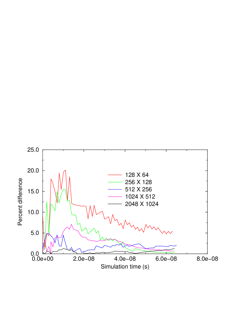
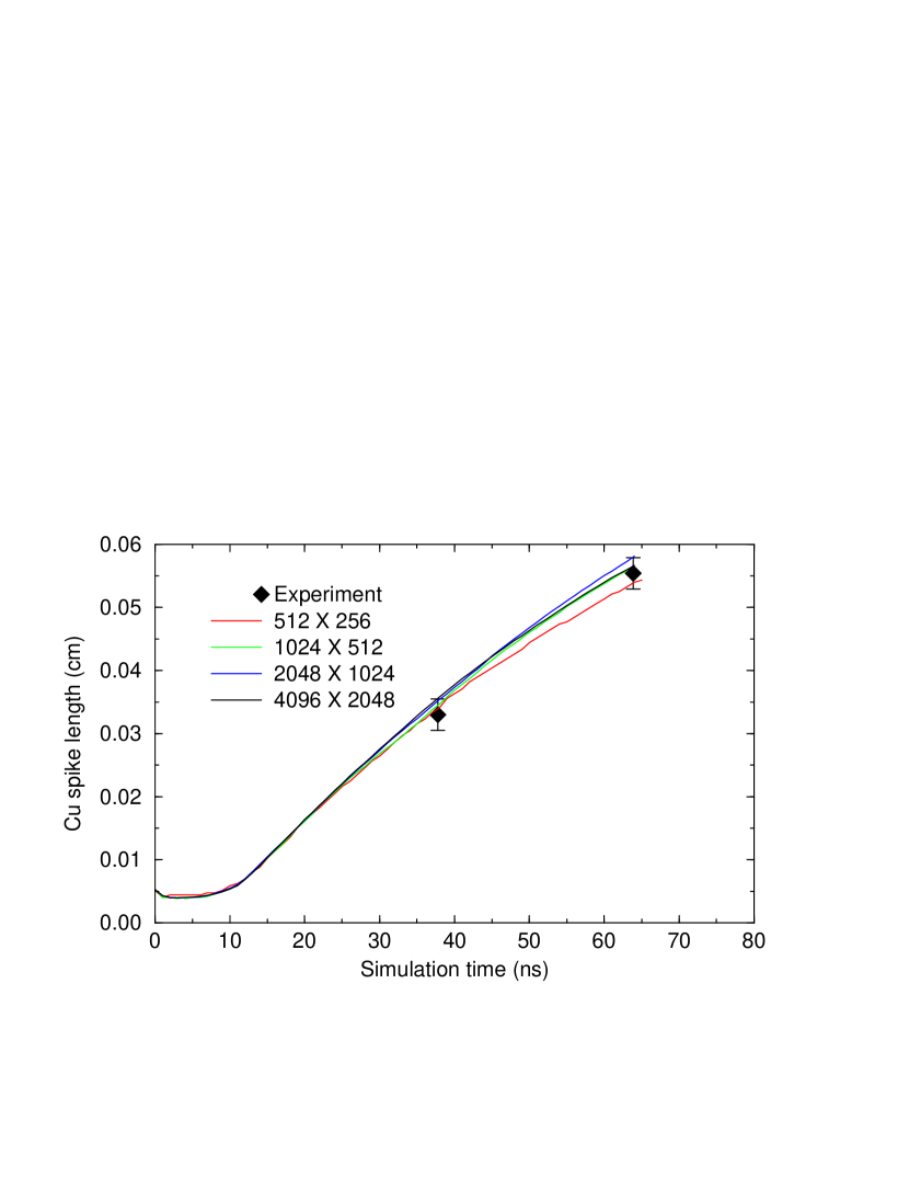
Figure 5 shows the Cu spike length vs. time for 4 simulations at increasing resolution. Also shown are the above-mentioned experimental results. The experimental error bars correspond to , the spatial error of the experiment. The width of the symbols marking the experimental results indicates approximately the timing error. The figure shows that the simulations quantitatively agree with the experimental results at the early and late times to within the experimental uncertainty.
4.3 Computation of Reaction Products in Large Eddy Simulations of Supernovae
When a laboratory experiment is available, the distinction between verification and validation is fairly clear, as discussed earlier. However, when creating predictive simulations of astrophysical processes that cannot be reproduced directly in the laboratory, even using appropriate scaling laws, the distinction can become less clear because the task becomes one of confirmation of simulation results without laboratory results. In many situations, notably in stellar combustion, it is possible to have a model that is demonstrably more physically valid but is too expensive or constrained to be used for the desired predictive simulations. Simpler models must be applied to simulate observed phenomena, hence the need for comparison of different methods.
Nuclear reaction networks and multi-dimensional simulations present a good example of this confluence of verification and validation. In astrophysical detonations it is possible to compute the steady-state structure of the propagating reaction front with a large reaction network with hundreds of species and thousands of reactions using error-controlled numerical methods (e.g. Sharpe, 1999; Moore et al, 2013) Consider the following question: How many species are necessary to accurately predict the characteristics of the flow such as peak temperature and reaction front width? This is not a verification question. We can use verification techniques to demonstrate that the equations governing the time integration of the reactions are being solved to a desired accuracy. Such a test, however, does not demonstrate whether or not a particular selection of species is sufficient for the stated purpose. So we proceed to compare our model with say three or a dozen “effective” reactions or species to another model which we believe to be more physically valid because it has more complete reaction physics. This situation is neither verification that our model is being solved correctly (that is already done) nor is it validation against a specific physical experiment. It is, however, validation under the definition introduced in section 2 above, in that it addresses whether the model is physically correct. Some terminology refers to this as confirmation of one model with a physically more valid model. Since the label depends finely on definitions of terminology, it is useful in discussion to term this type of comparison as something that combines elements of verification and validation (see Ch. 41 by Beisbart in this volume). It is a model-to-model comparison, as verification often is, but addresses the physical applicability of the model, as validation does.
If integration of thousands of reactions were the only issue, this validation of simplified models might not be worthwhile; instead one would just use the better model directly. There are areas of prediction, however, where direct use of the better model can be infeasible. In explosive astrophysical combustion (which powers type Ia supernova explosions), it is typically desirable to predict the overall products and the speeds at which they are ejected. Unfortunately, a simulation that can predict that information must include the entire star, which may be around cm in size. The reaction front through which the combustion takes place is one cm or less in thickness (Townsley et al, 2016). Also, the propagation of this front through the star will generally occur in a way that obeys no particularly symmetry, making it necessary to simulate this combustion and ejection of material in three dimensions.
The necessity of simulating the whole star in three dimensions presents several challenges from the standpoint of V&V. First, since the combustion phenomena occur far below the best possible grid scale ( cm), the typical method of verification by convergence study is not valid. Claiming convergence for a numerical solution of differential equations presupposes that the relevant gradients are numerically resolved and become better resolved at higher resolution. This is the very meaning of resolution. However, in the full-scale astrophysical case, an example of the above-mentioned large eddy simulation situation, the composition gradients representing the physical reaction front (the length scale over which the fuel is consumed and converted to products) are never actually resolved. Secondly, while error-controlled methods for ODE integration are well-understood, similar automated control of accuracy is not available in current widely used methods for solution of PDEs, such as in hydrodynamics. Because this control is not built into the method, performing predictive simulations involves a constant process of verification to ensure that solutions obtained do not depend on resolution. That process can be both expensive and time-consuming. Thirdly, it may be computationally infeasible to include hundreds of species and thousands of reactions in the full-scale hydrodynamic simulation, thus even if we were able to verify the methods for reactive hydrodynamics, we would need to use a model for the reactions that we know to have specific deficiencies and would therefore need some form of validation against more physically complete models. Finally, as discussed earlier, because some physical processes such as fluid dissipation due to viscosity is left implicit, a higher-resolution simulation may not only be more numerically accurate but also more physically valid. As a result of these issues, verification and validation of the simulation of a stellar explosion can be mixed in a way that is not always cleanly separable.
Here we will present a discussion of ongoing efforts at verification and validation of methods for computing the products of thermonuclear supernova explosions. The full-star simulations use a simplified model of the reactions for computational efficiency, and are necessarily under-resolved. The overall goal is to compare the results from this computational model to computational models of much higher physical and numerical fidelity. In the case of combustion, those are computations with large, complete nuclear reaction networks computed using resolved, error-controlled numerical techniques. The limitation is that the latter methods can only be used under certain flow conditions, specifically, a steady state. We therefore proceed by treating the methods used in the full-star simulation as the model to be validated by comparison to more physical calculations. This is similar to verification by comparison to a benchmark, except that the two models are known to be different by construction.
Table 1 shows a matrix comparing the capabilities of compressible hydrodynamics simulations in various dimensions as well as the fully resolved method, which can only be used in one dimension and for reaction fronts propagating in a steady state through a uniform medium. As shown, a resolved calculation with the full network at all densities relevant to the supernova can only be performed with the steady-state method. However, this method cannot be used to treat transients (e.g. ignition or non-spatially uniform density) or general geometries including the full star. Of the hydrodynamical methods in various spatial dimensions, represented in the other three columns of the table, only one-dimensional calculations can use a full reaction network effectively and resolve the reaction front, though not at all densities. The possible importance of transient effects necessitates a multi-step strategy utilizing cross-comparisons of calculations of reaction front structure among several different methods. For example, we can verify one-dimensional dynamical calculations at uniform densities using comparison to steady-state calculations, and then use one-dimensional calculations with non-uniform density to characterize transient effects. Even for a transient, it is informative to compare to steady-state solutions in order to provide physical insight to the importance of non-uniformities in density.
| Capability | 3-d | 2-d | 1-d | 1-d steady |
| full reaction network | ✓ | ✓ | ||
| resolved at low density | ✓ | ✓ | ||
| resolved at high density | ✓ | |||
| transients (dynamical) | ✓ | ✓ | ✓ | |
| general geometries | ✓ | |||
| full star | ✓ | ✓ | ✓ |
Figure 6 shows an example of a comparison of the compositional structure of a propagating detonation reaction front computed with the one-dimensional dynamical method and the one-dimensional steady-state method. The hydrodynamical simulation (dashed lines) was performed at a physical resolution of cm, which corresponds to a hydrodynamical time step of about s. The fuel here is mostly 12C and 16O, which is reacted to eventually become 56Ni. The consumption of 12C is not shown, but is even faster than that of 16O. The structure for a detonation propagating in steady state (solid lines) is computed with an error-controlled method using adaptive time stepping and an error tolerance of order , and is therefore suitably resolved by construction. The abundance histories from the hydrodynamical model shown here are the result of using a simplified reaction model in the hydrodynamics and then post-processing the resulting density and temperature histories of fluid elements with a larger reaction network (Travaglio et al, 2004; Townsley et al, 2016). The goal of this comparison is to validate that away from the unresolved portion of the reaction front (timescales s), the composition history is accurately predicted by the under-resolved calculation with the simplified burning model. This comparison shows that the results are in good agreement for steady-state, planar detonations. For an example of a comparison for non-planar (curved) detonations see Moore et al (2013).
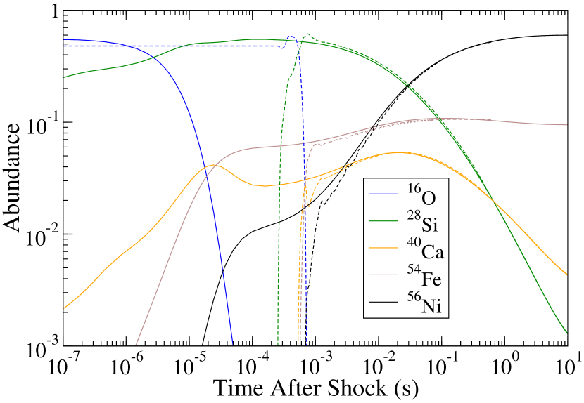
of magnitude higher resolution in the hydrodynamic simulation.
The validation of methods for computing astrophysical combustion in large eddy simulations is ongoing. The various possible calculations represented in Table 1 must be compared for geometries and conditions for which there is overlap in capability. This process also entails ongoing improvement of both the simplified reaction model utilized in the large eddy simulations (Townsley et al, 2009; Willcox et al, 2016) as well as improving techniques for computing the final yields (Townsley et al, 2016).
5 Discussion
The simulational results for the hydrodynamics validation example fell within the temporal and spatial error bars of the experimental results thus showing quantitative agreement between simulation and experiment for the metric of the lengths of the copper spikes. This agreement demonstrates that the hydrodynamics module in Flash captured the bulk properties of the flow and observable morphology. and builds confidence in simulations of astrophysical phenomena. We cannot, however, declare the code “validated” for a host of reasons:
-
•
The experimental configuration produced essentially a two-dimensional result, hence our modeling it with two-dimensional simulations. The experiment was three-dimensional, so correctly describing the fluid instabilities, particularly the amount of small-scale structure in the flow may require three-dimensional simulations.
-
•
The models were incomplete. The three materials were modeled as ideal gasses, a questionable assumption. Also, for convenience, the simulations neglected the presence of the shock tube surrounding the target and assumed periodic boundary conditions. Thus the simulations did not include effects due to the shock tube.
-
•
The experimental diagnostics, radiographs, are really shadows that cannot adequately capture small-scale structure. Even if three-dimensional simulations that better described the fluid instabilities had been performed, comparison to the experimental results is limited by the experimental diagnostics.
-
•
The observed degraded agreement between simulations at the highest resolutions indicates the results are not converged. We attribute this result to the fact that the Euler equations allow a changing numerical viscosity with resolution, which changes the Reynolds number and thus the nature of any turbulence. Additional commentary on this issue may be found in Calder et al (2002).
Even with limitations, the demonstrated ability of the simulations to capture the expected bulk properties of the flow builds confidence in the results of astrophysical simulations, allowing us to conclude that the shocks and fluid instabilities study was a success. The principal differences observed between the results from simulations and the experimental results were in the amount of small scale structure observed in the flow, with the amount of small-scale structure in the simulations increasing with resolution. This behavior is expected because the effective Reynolds number increases with resolution as described above, and we believe this effect is the source of the observed imperfect convergence. Because the experimental data are radiographs and cannot capture the actual amount of small-scale structure in the flow, the correct amount of small-scale structure remains undetermined and even if the convergence of the simulations had been perfect, we could not conclude the solution converged to the correct result.
In addition to increasing confidence in the results, the hydrodynamics validation study was well worth the investment because of the lessons learned in comparing the experimental and simulational results. The collaborative process of determining the metric for comparison and extracting the results from the experimental and simulational data resulted in a better understanding of the issues, which also increases confidence in the astrophysical results. The experimentalists also benefited from the process of validation because the process of comparison suggested metrics for future comparisons, provided useful diagnostics, and supplied a virtual model that aided in the design of future experiments. A point worth stressing again in conclusion is the importance of close collaboration between the experimentalists and theorists needed to make a meaningful quantitative comparison. Raw experimental data such as a radiograph alone does not allow for a quantitative comparison to simulational results. Finally, we note that the success of this collaboration seeded interest in high energy density physics among the developers of Flash, which subsequently resulted in an extended course of collaborative research into high energy density physics (see Tzeferacos et al (2015) and references therein).
The product of reactive hydrodynamics study gave a look at the process of comparing models of differing fidelity to ensure that macroscopic (three-dimensional) simulations capture the physics of thermonuclear reactions while also allowing the calculation of detailed abundances. Our approach is to test simplified models against higher-fidelity models for a given physical process, here thermonuclear combustion. Simplified models then facilitate three-dimensional simulations that would be intractable otherwise. The results of these studies are also applicable to the problem of determining detailed abundances from the density and temperature histories of Lagrangian tracers. We illustrated this process with a comparison between results from post-processed tracers from a hydrodynamics simulation and a detailed calculation of steady-state burning structure. This study confirmed that our simulations capture the essence of the reactions in whole-star models, and thereby increased confidence in our predictions of the astrophysical events.
6 Conclusions
The cases we present here are but one part of the continuing effort at verifying and validating Flash and associated infrastructure (e.g. the post-processing method presented here). The first study of validating the hydrodynamics was performed early in the development of Flash. Though very informative, it could have been continued further with additional quantification of the effect of missing physics as a good next step. Also, further modifications to the code would allow it to capture high energy density phenomena better. Such activities, however, were not critical to the astrophysical problems. Still, the case was very informative and served to increase confidence in the results. The second case, the computation of reaction products in large eddy simulations of supernovae, is very much a work in progress and represents our contemporary effort.
Our conclusion from both of these studies is that like any discipline in computational science, V&V are an essential part of the process of modeling astrophysical phenomena. V&V in astrophysics can be particularly challenging due to the inaccessibility of the physical conditions attained and limited ancillary measurements available for distant events. As shown here by these examples, however, positive steps that build confidence in models can be taken based on comparisons using related laboratory experiments and more complete physical models where available.
Acknowledgements.
This contribution was supported in part by the Department of Energy through grant DE-FG02-87ER40317 and the research described here was supported in part by earlier grant B341495 to the Center for Astrophysical Flashes at the University of Chicago. The software used in this work was in part developed by the DOE-supported ASC/Alliances Center for Astrophysical Thermonuclear Flashes at the University of Chicago. This research has made use of NASA’s Astrophysics Data System. The authors thank Eric Winsberg and Bruce Fryxell for helpful discussions about this manuscript.References
- AIAA (1998) AIAA (1998) Guide for the Verification and Validation of Computational Fluid Dynamics Simulations. AIAA Report G-077-1998; Reston, VA: American Institute of Aeronautics and Astronautics
- Alexakis et al (2004) Alexakis A, Calder AC, Heger A, Brown EF, Dursi LJ, Truran JW, Rosner R, Lamb DQ, Timmes FX, Fryxell B, Zingale M, Ricker PM, Olson K (2004) On Heavy Element Enrichment in Classical Novae. Astrophysical Journal 602:931–937, DOI 10.1086/381086, astro-ph/0307126
- AMReX (2018) AMReX, 2018, https://amrex-codes.github.io/, freely available
- Arnett et al (1989) Arnett D, Fryxell B, Mueller E (1989) Instabilities and nonradial motion in SN 1987A. Astrophysical Journal Letters 341:L63–L66, DOI 10.1086/185458
- Blottner (1990) Blottner FG (1990) Accurate navier-stokes results for the hypersonic flow over a spherical nosetip. Journal of Spacecraft and Rockets 27(2):113–122, also AIAA Paper 89–0269, Jan. 1989
- Boehly et al (1995) Boehly TR, Craxton RS, Hinterman TH, Kelly JH, Kessler TJ, Kumpan SA, Letzring SA, McCrory RL, Morse SFB, Seka W, Skupsky S, Soures JM, Verdon CP (1995) The upgrade to the OMEGA laser system. Review of Scientific Instruments 66:508–510, DOI 10.1063/1.1146333
- Boehm (1981) Boehm BW (1981) Software Engineering Economics, 1st edn. Prentice Hall PTR, Upper Saddle River, NJ, USA
- Bradley et al (1998) Bradley DK, Delettrez JA, Epstein R, Town RPJ, Verdon CP, Yaakobi B, Regan S, Marshall FJ, Boehly TR, Knauer JP, Meyerhofer DD, Smalyuk VA, Seka W, Haynes DA, Gunderson M, Junkel G, Hooper CF, Bell PM, Ognibene TJ, Lerche RA (1998) Measurements of core and pusher conditions in surrogate capsule implosions on the OMEGA laser system. Physics of Plasmas 5:1870–1879, DOI 10.1063/1.872858
- Calder (2005) Calder AC (2005) Laboratory Astrophysics Experiments for Simulation Code Validation: A Case Study. Astrophysics and Space Science 298:25–32, DOI 10.1007/s10509-005-3908-2
- Calder et al (2000) Calder AC, Curtis BC, Dursi LJ, Fryxell B, Henry G, MacNeice P, Olson K, Ricker P, Rosner R, Timmes FX, Tufo HM, Truran JW, Zingale M (2000) High-performance reactive fluid flow simulations using adaptive mesh refinement on thousands of processors. In: Proceedings of Supercomputing 2000, p http://sc2000.org
- Calder et al (2002) Calder AC, Fryxell B, Plewa T, Rosner R, Dursi LJ, Weirs VG, Dupont T, Robey HF, Kane JO, Remington BA, Drake RP, Dimonte G, Zingale M, Timmes FX, Olson K, Ricker P, MacNeice P, Tufo HM (2002) On validating an astrophysical simulation code. Astrophysical Journal Supplement Series 143:201–229
- Calder et al (2006) Calder AC, Taylor NT, Antypas K, Sheeler D, Dubey A (2006) A Case Study of Verifying and Validating an Astrophysical Simulation Code. In: Zank GP, Pogorelov NV (eds) Numerical Modeling of Space Plasma Flows, Astronomical Society of the Pacific Conference Series, vol 359, p 119
- Calder et al (2007) Calder AC, Townsley DM, Seitenzahl IR, Peng F, Messer OEB, Vladimirova N, Brown EF, Truran JW, Lamb DQ (2007) Capturing the Fire: Flame Energetics and Neutronization for Type Ia Supernova Simulations. Astrophysical Journal 656:313–332, DOI 10.1086/510709, astro-ph/0611009
- Calder et al (2013) Calder AC, Krueger BK, Jackson AP, Townsley DM (2013) The influence of chemical composition on models of Type Ia supernovae. Frontiers of Physics 8:168–188, DOI 10.1007/s11467-013-0301-4, 1303.2207
- Calder et al (2018) Calder AC, Hoffman MM, Willcox DE, Katz MP, Swesty FD, Ferson S (2018) Quantification of incertitude in black box simulation codes. Journal of Physics: Conference Series 1031(1):012,016, URL http://stacks.iop.org/1742-6596/1031/i=1/a=012016
- Chandrasekhar (1981) Chandrasekhar S (1981) Hydrodynamic and Hydromagnetic Stability. Dover, New York
- Colella and Glaz (1985) Colella P, Glaz HM (1985) Efficient solution algorithms for the Riemann problem for real gases. Journal of Computational Physics 59:264–289, DOI 10.1016/0021-9991(85)90146-9
- Colella and Woodward (1984) Colella P, Woodward PR (1984) The Piecewise Parabolic Method (PPM) for Gas-Dynamical Simulations. Journal of Computational Physics 54:174–201
- Dubey et al (2009) Dubey A, Antypas K, Ganapathy MK, Reid LB, Riley K, Sheeler D, Siegel A, Weide K (2009) Extensible component-based architecture for flash, a massively parallel, multiphysics simulation code. Parallel Computing 35(10–11):512 – 522, DOI https://doi.org/10.1016/j.parco.2009.08.001, URL http://www.sciencedirect.com/science/article/pii/S0167819109000945
- Dubey et al (2013) Dubey A, Calder AC, Daley C, Fisher RT, Graziani C, Jordan GC, Lamb DQ, Reid LB, Townsley DM, Weide K (2013) Pragmatic optimizations for better scientific utilization of large supercomputers. The International Journal of High Performance Computing Applications 27(3):360–373, DOI 10.1177/1094342012464404, URL http://dx.doi.org/10.1177/1094342012464404
- Dubey et al (2014) Dubey A, Antypas K, Calder AC, Daley C, Fryxell B, Gallagher JB, Lamb DQ, Lee D, Olson K, Reid LB, Rich P, Ricker PM, Riley KM, Rosner R, Siegel A, Taylor NT, Weide K, Timmes FX, Vladimirova N, ZuHone J (2014) Evolution of flash, a multi-physics scientific simulation code for high-performance computing. The International Journal of High Performance Computing Applications 28(2):225–237, DOI 10.1177/1094342013505656, URL http://dx.doi.org/10.1177/1094342013505656
- Dubey et al (2015) Dubey A, Weide K, Lee D, Bachan J, Daley C, Olofin S, Taylor N, Rich PM, Reid LB (2015) Ongoing verification of a multiphysics community code: Flash. Software: Practice and Experience 45(2):233–244, DOI 10.1002/spe.2220, URL http://dx.doi.org/10.1002/spe.2220
- Dwarkadas et al (2005) Dwarkadas V, Plewa T, Weirs G, Tomkins C, Marr-Lyon M (2005) Simulation of Vortex-Dominated Flows Using the FLASH Code, Springer Berlin Heidelberg, Berlin, Heidelberg, pp 527–537. DOI 10.1007/3-540-27039-6˙39, URL http://dx.doi.org/10.1007/3-540-27039-6_39
- Encyclopaedia Britannica (2006) Encyclopaedia Britannica, 2006, https://www.britannica.com/science/eddy-fluid-mechanics
- Fryxell et al (1991) Fryxell B, Arnett D, Mueller E (1991) Instabilities and clumping in SN 1987A. I - Early evolution in two dimensions. Astrophysical Journal 367:619–634, DOI 10.1086/169657
- Fryxell et al (2000) Fryxell B, Olson K, Ricker P, Timmes FX, Zingale M, Lamb DQ, MacNeice P, Rosner R, Truran JW, Tufo H (2000) FLASH: An adaptive mesh hydrodynamics code for modeling astrophysical thermonuclear flashes. Astrophysical Journal Supplement Series 131:273–334
- Fryxell et al (1989) Fryxell BA, Müller E, Arnett D (1989) Hydrodynamics and nuclear burning. MPIA Technical Report
- Fureby (1996) Fureby C (1996) On subgrid scale modeling in large eddy simulations of compressible fluid flow. Physics of Fluids 8(5):1301–1311, DOI 10.1063/1.868900, URL https://doi.org/10.1063/1.868900
- Gamboa et al (2012) Gamboa EJ, Huntington CM, Trantham MR, Keiter PA, Drake RP, Montgomery DS, Benage JF, Letzring SA (2012) Imaging x-ray thomson scattering spectrometer design and demonstration (invited). Review of Scientific Instruments 83(10):10E108, DOI 10.1063/1.4731755, URL http://dx.doi.org/10.1063/1.4731755
- Gamboa et al (2014) Gamboa EJ, Drake RP, Falk K, Keiter PA, Montgomery DS, Benage JF, Trantham MR (2014) Simultaneous measurements of several state variables in shocked carbon by imaging x-ray scattering. Physics of Plasmas 21(4):042,701, DOI 10.1063/1.4869241, URL http://dx.doi.org/10.1063/1.4869241
- Godunov et al (1962) Godunov S, Zabrodin A, Prokopov G (1962) A computational scheme for two-dimensional non stationary problems of gas dynamics and calculation of the flow from a shock wave approaching a stationary state. USSR Computational Mathematics and Mathematical Physics 1(4):1187 – 1219, DOI https://doi.org/10.1016/0041-5553(62)90039-3, URL http://www.sciencedirect.com/science/article/pii/0041555362900393
- Godunov (1959) Godunov SK (1959) A difference scheme for numerical solution of discontinuous solution of hydrodynamic equations. Math Sbornik 47:271–306, URL https://ci.nii.ac.jp/naid/10029009112/en/
- Grinstein et al (2007) Grinstein F, Margolin L, Rider W (2007) Implicit Large Eddy Simulation: Computing Turbulent Fluid Dynamics. Cambridge University Press
- Hearn et al (2007) Hearn NC, Plewa T, Drake RP, Kuranz C (2007) Flash Code Simulations of Rayleigh-Taylor and Richtmyer-Meshkov Instabilities in Laser-Driven Experiments. Astrophysics and Space Science 307:227–231, DOI 10.1007/s10509-006-9226-5
- Hoffman et al (2018) Hoffman MM, Willcox DE, Katz MP, Ferson S, Swesty FD, Calder AC (2018) On the quantification of incertitude in astrophysical simulation codes. Astrophysical Journal In preparation
- Kane et al (2001) Kane JO, Robey HF, Remington BA, Drake RP, Knauer J, Ryutov DD, Louis H, Teyssier R, Hurricane O, Arnett D, Rosner R, Calder A (2001) Interface imprinting by a rippled shock using an intense laser. Physical Review E 63(5):055,401–+, DOI 10.1103/PhysRevE.63.055401
- Kritsuk et al (2006) Kritsuk AG, Norman ML, Padoan P (2006) Adaptive Mesh Refinement for Supersonic Molecular Cloud Turbulence. Astrophysical Journal Letters 638:L25–L28, DOI 10.1086/500688, astro-ph/0411626
- Larsen and Lane (1994) Larsen JT, Lane SM (1994) Hyades–A plasma hydrodynamics code for dense plasma studies. JQSRT 51:179–186, DOI 10.1016/0022-4073(94)90078-7
- Lee (2013) Lee D (2013) A solution accurate, efficient and stable unsplit staggered mesh scheme for three dimensional magnetohydrodynamics. Journal of Computational Physics 243:269 – 292, DOI http://dx.doi.org/10.1016/j.jcp.2013.02.049, URL http://www.sciencedirect.com/science/article/pii/S0021999113001836
- Lee and Deane (2009) Lee D, Deane AE (2009) An unsplit staggered mesh scheme for multidimensional magnetohydrodynamics. Journal of Computational Physics 228(4):952 – 975, DOI http://dx.doi.org/10.1016/j.jcp.2008.08.026, URL http://www.sciencedirect.com/science/article/pii/S0021999108004506
- Lee et al (2017a) Lee D, Faller H, Reyes A (2017a) The piecewise cubic method (pcm) for computational fluid dynamics. Journal of Computational Physics 341:230 – 257, DOI https://doi.org/10.1016/j.jcp.2017.04.004, URL http://www.sciencedirect.com/science/article/pii/S0021999117302759
- Lee et al (2017b) Lee D, Tzeferacos P, Couch S, Bachan J, Daley C, Fatehejad M, Flocke N, Graziani C, Lamb D, Weide K, Dubey A (2017b) Flash: a multi-physics code for adaptive mesh computational fluid dynamics in astrophysics. Astrophysical Journal In preparation
- Li (2010) Li S (2010) Comparison of refinement criteria for structured adaptive mesh refinement. Journal of Computational and Applied Mathematics 233(12):3139 – 3147, DOI https://doi.org/10.1016/j.cam.2009.08.104, URL http://www.sciencedirect.com/science/article/pii/S037704270900586X, finite Element Methods in Engineering and Science (FEMTEC 2009)
- Li and Wood (2017) Li Z, Wood R (2017) Accuracy verification of a 2d adaptive mesh refinement method for incompressible or steady flow. J Comput Appl Math 318(C):259–265, DOI 10.1016/j.cam.2016.09.022, URL https://doi.org/10.1016/j.cam.2016.09.022
- MacNeice et al (1999) MacNeice P, Olson C K M Mobarry, de Fainchtein R, Packer C (1999) Paramesh: A parallel adaptive mesh refinement community toolkit. NASA Tech Rep CR-1999-209483
- MacNeice et al (2000) MacNeice P, Olson C K M Mobarry, de Fainchtein R, Packer C (2000) Paramesh: A parallel adaptive mesh refinement community toolkit. Comput Phys Commun 126:330–354
- Majda (1984) Majda A (1984) Compressible Fluid Flow and Systems of Conservation Laws in Several Space Variables
- Margolin (2014) Margolin L (2014) Finite scale theory: The role of the observer in classical fluid flow. Mechanics Research Communications 57:10 – 17, DOI http://dx.doi.org/10.1016/j.mechrescom.2013.12.004, URL http://www.sciencedirect.com/science/article/pii/S009364131300205X
- Margolin and Rider (2002) Margolin LG, Rider WJ (2002) A rationale for implicit turbulence modelling. International Journal for Numerical Methods in Fluids 39(9):821–841, DOI 10.1002/fld.331, URL http://dx.doi.org/10.1002/fld.331
- Margolin and Shashkov (2008) Margolin LG, Shashkov M (2008) Finite volume methods and the equations of finite scale: A mimetic approach. International Journal for Numerical Methods in Fluids 56(8):991–1002, DOI 10.1002/fld.1592, URL http://dx.doi.org/10.1002/fld.1592
- Meshkov (1969) Meshkov EE (1969) Instability of the interface of two gases accelerated by a shock wave. Izv Acad Sci USSR Fluid Dyn 4:101
- Miles et al (2016) Miles BJ, van Rossum DR, Townsley DM, Timmes FX, Jackson AP, Calder AC, Brown EF (2016) On Measuring the Metallicity of a Type Ia Supernova’s Progenitor. Astrophysical Journal824:59, DOI 10.3847/0004-637X/824/1/59, 1508.05961
- Mitran (2009) Mitran SM (2009) Adaptive Mesh Refinement Computation of Turbulent Flows – Pitfalls and Escapes. In: Pogorelov NV, Audit E, Colella P, Zank GP (eds) Numerical Modeling of Space Plasma Flows: ASTRONUM-2008, Astronomical Society of the Pacific Conference Series, vol 406, p 249
- Moore et al (2013) Moore K, Townsley DM, Bildsten L (2013) The Effects of Curvature and Expansion on Helium Detonations on White Dwarf Surfaces. Astrophysical Journal776:97, DOI 10.1088/0004-637X/776/2/97, 1308.4193
- Muller et al (1989) Muller E, Hillebrandt W, Orio M, Hoflich P, Monchmeyer R, Fryxell BA (1989) Mixing and fragmentation in supernova envelopes. Astronomy and Astrophysics220:167–176
- Oberkampf and Roy (2010) Oberkampf W, Roy C (2010) Verification and Validation in Scientific Computing. Cambridge University Press
- Plewa et al (2004) Plewa T, Calder AC, Lamb DQ (2004) Type Ia Supernova Explosion: Gravitationally Confined Detonation. Astrophysical Journal Letters 612:L37–L40, DOI 10.1086/424036, astro-ph/0405163
- Richtmyer (1960) Richtmyer RD (1960) Taylor instability in shock acceleration of compressible fluids. Communications on Pure and Applied Mathematics 13(2):297–319, DOI 10.1002/cpa.3160130207, URL http://dx.doi.org/10.1002/cpa.3160130207
- Roache (1998a) Roache P (1998a) Verification and Validation in Computational Science and Engineering. Hermosa
- Roache (1998b) Roache PJ (1998b) Fundamentals of Computational Fluid Dynamics. Hermosa, Albuquerque, USA
- Robey et al (2001) Robey HF, Kane JO, Remington BA, Drake RP, Hurricane OA, Louis H, Wallace RJ, Knauer J, Keiter P, Arnett D, Ryutov DD (2001) An experimental testbed for the study of hydrodynamic issues in supernovae. Physics of Plasmas 8(5):2446–2453, DOI 10.1063/1.1352594, URL http://dx.doi.org/10.1063/1.1352594
- Rosner et al (2000) Rosner R, Calder AC, Dursi LJ, Fryxell B, Lamb DQ, Niemeyer JC, Olson K, Ricker P, Timmes FX, Truran JW, Tufo H, Young Y, Zingale M, Lusk E, Stevens R (2000) Flash Code: Studying Astrophysical Thermonuclear Flashes. Computing in Science and Engineering 2:33
- Sharpe (1999) Sharpe GJ (1999) The structure of steady detonation waves in Type Ia supernovae: pathological detonations in C-O cores. Monthly Notices of the Royal Astronomical Society310:1039–1052, DOI 10.1046/j.1365-8711.1999.03023.x
- Shu et al (2017) Shu Q, Ateljevich E, Schwartz PO, Colella P (2017) Verification of an Adaptive Mesh, Embedded Boundary Model for Flood Modeling Applications. DOI 10.1061/41173(414)229, URL http://ascelibrary.org/doi/abs/10.1061/41173%28414%29229
- Soures et al (1996) Soures JM, McCrory RL, Verdon CP, Babushkin A, Bahr RE, Boehly TR, Boni R, Bradley DK, Brown DL, Craxton RS, Delettrez JA, Donaldson WR, Epstein R, Jaanimagi PA, Jacobs SD, Kearney K, Keck RL, Kelly JH, Kessler TJ, Kremens RL, Knauer JP, Kumpan SA, Letzring SA, Lonobile DJ, Loucks SJ, Lund LD, Marshall FJ, McKenty PW, Meyerhofer DD, Morse SFB, Okishev A, Papernov S, Pien G, Seka W, Short R, Shoup MJ, Skeldon M, Skupsky S, Schmid AW, Smith DJ, Swales S, Wittman M, Yaakobi B (1996) Direct-drive laser-fusion experiments with the OMEGA, 60-beam, greater than 40 kJ, ultraviolet laser system. Physics of Plasmas 3:2108–2112, DOI 10.1063/1.871662
- Stoeckl et al (2012) Stoeckl C, Fiksel G, Guy D, Mileham C, Nilson PM, Sangster TC, III MJS, Theobald W (2012) A spherical crystal imager for omega ep. Review of Scientific Instruments 83(3):033,107, DOI 10.1063/1.3693348, URL http://dx.doi.org/10.1063/1.3693348
- Storer (2017) Storer T (2017) Bridging the chasm: A survey of software engineering practice in scientific programming. ACM Comput Surv 50(4):47:1–47:32, DOI 10.1145/3084225, URL http://doi.acm.org/10.1145/3084225
- Taylor (1950) Taylor G (1950) The Instability of Liquid Surfaces when Accelerated in a Direction Perpendicular to their Planes. I. Royal Society of London Proceedings Series A 201:192–196
- Timmes et al (2004) Timmes F, Dimonte G, Kane J, Fryxell B, Olson K, Plewa T, Hayes J, Robey H, Stone J, Dupont T, Calder A, Dursi J, Ricker P, Zingale M, Remington B, Weirs G, Drake P (2004) Validating astrophysical simulation codes. Computing in Science and Engineering 6:10–20, DOI doi.ieeecomputersociety.org/10.1109/MCSE.2004.44
- Townsley et al (2007) Townsley DM, Calder AC, Asida SM, Seitenzahl IR, Peng F, Vladimirova N, Lamb DQ, Truran JW (2007) Flame Evolution During Type Ia Supernovae and the Deflagration Phase in the Gravitationally Confined Detonation Scenario. Astrophysical Journal 668:1118–1131, DOI 10.1086/521013, 0706.1094
- Townsley et al (2009) Townsley DM, Jackson AP, Calder AC, Chamulak DA, Brown EF, Timmes FX (2009) Evaluating Systematic Dependencies of Type Ia Supernovae: The Influence of Progenitor 22Ne Content on Dynamics. Astrophysical Journal701:1582–1604, DOI 10.1088/0004-637X/701/2/1582, 0906.4384
- Townsley et al (2016) Townsley DM, Miles BJ, Timmes FX, Calder AC, Brown EF (2016) A Tracer Method for Computing Type Ia Supernova Yields: Burning Model Calibration, Reconstruction of Thickened Flames, and Verification for Planar Detonations. Astrophysical Journal Supplement Series 225:3, DOI 10.3847/0067-0049/225/1/3, 1605.04878
- Travaglio et al (2004) Travaglio C, Hillebrandt W, Reinecke M, Thielemann FK (2004) Nucleosynthesis in multi-dimensional SN Ia explosions. Astronomy and Astrophysics425:1029–1040, DOI 10.1051/0004-6361:20041108, astro-ph/0406281
- Tzeferacos et al (2015) Tzeferacos P, Fatenejad M, Flocke N, Graziani C, Gregori G, Lamb D, Lee D, Meinecke J, Scopatz A, Weide K (2015) {FLASH} {MHD} simulations of experiments that study shock-generated magnetic fields. High Energy Density Physics 17, Part A:24 – 31, DOI https://doi.org/10.1016/j.hedp.2014.11.003, URL http://www.sciencedirect.com/science/article/pii/S1574181814000779, 10th International Conference on High Energy Density Laboratory Astrophysics
- van der Holst et al (2011) van der Holst B, Tóth G, Sokolov IV, Powell KG, Holloway JP, Myra ES, Stout Q, Adams ML, Morel JE, Karni S, Fryxell B, Drake RP (2011) CRASH: A Block-adaptive-mesh Code for Radiative Shock Hydrodynamics—Implementation and Verification. Astrophysical Journal Supplement Series 194:23, DOI 10.1088/0067-0049/194/2/23, 1101.3758
- Weirs et al (2005) Weirs G, Dwarkadas V, Plewa T, Tomkins C, Marr-Lyon M (2005) Validating the Flash Code: Vortex-Dominated Flows. Astrophysics and Space Science 298:341–346, DOI 10.1007/s10509-005-3966-5, astro-ph/0405410
- Weirs et al (2005) Weirs G, Dwarkadas V, Plewa T, Tomkins C, Marr-Lyon M (2005) Validating the Flash Code: Vortex-Dominated Flows, Springer Netherlands, Dordrecht, pp 341–346. DOI 10.1007/1-4020-4162-4˙51, URL http://dx.doi.org/10.1007/1-4020-4162-4_51
- Willcox et al (2016) Willcox DE, Townsley DM, Calder AC, Denissenkov PA, Herwig F (2016) Type Ia Supernova Explosions from Hybrid Carbon-Oxygen-Neon White Dwarf Progenitors. Astrophysical Journal832:13, DOI 10.3847/0004-637X/832/1/13, %****␣ms.tex␣Line␣1825␣****1602.06356
- Winsberg (2010) Winsberg E (2010) Science in the Age of Computer Simulation. University of Chicago Press
- Zhang et al (2007) Zhang J, Messer OEB, Khokhlov AM, Plewa T (2007) On the Evolution of Thermonuclear Flames on Large Scales. Astrophysical Journal 656:347–365, DOI 10.1086/510145, astro-ph/0610168
- Zhiyin (2015) Zhiyin Y (2015) Large-eddy simulation: Past, present and the future. Chinese Journal of Aeronautics 28(1):11 – 24, DOI https://doi.org/10.1016/j.cja.2014.12.007, URL http://www.sciencedirect.com/science/article/pii/S1000936114002064
- Zingale et al (2001) Zingale M, Timmes FX, Fryxell B, Lamb DQ, Olson K, Calder AC, Dursi LJ, Ricker P, Rosner R, MacNeice P, Tufo HM (2001) Helium Detonations on Neutron Stars. Astrophysical Journal Supplement Series 133:195–220, DOI 10.1086/319182