Accurate and Efficient Numerical Simulation of Dielectrically Anisotropic Particles

Abstract

A variety of electrostatic phenomena, including the structure of electric double layers and the aggregation of charged colloids and proteins, are affected by nonuniform electric permittivity. These effects are frequently ignored in analytical and computational studies, and particularly difficult to handle in situations where multiple dielectric contrasts are present, such as in colloids that are heterogeneous in permittivity. We present an extension to the iterative dielectric solver developed by Barros and Luijten [Phys. Rev. Lett. 113, 017801 (2014)] that makes it possible to accurately compute the polarization of anisotropic particles with multiple dielectric contrasts. This efficient boundary-element method-based approach is applicable to geometries that are not amenable to other solvers, opening the possibility of studying collective phenomena of dielectrically anisotropic particles. We provide insight into the underlying physical reasons for this efficiency.

Electrostatic effects play a crucial role in colloidal suspensions, affecting their stabilization, aggregation, and electrokinetics.Levin (2002); Stradner et al. (2004); Linse and Lobaskin (1999); Morgan and Green (2003) Computer simulations can provide crucial insight in these electrostatic phenomena but owing to computational limitations typically resort to coarse-grained simulations, often using the so-called primitive model.Luijten, Fisher, and Panagiotopoulos (2002) This model treats colloids and ions as discrete particles but the background solvent as dielectric continuum. It is generally more accurate than mean-field techniques, since fluctuations and steric effects (i.e., finite ion size) are incorporated explicitly. However, since a colloid typically has a different electric permittivity than the surrounding solvent, it is also important to account for induced surface (polarization) charge. To resolve such effects in the primitive model, the dielectric heterogeneity must be included when solving Poisson’s equation, which is typically analytically complicated and numerically costly. Thus, polarization effects are ignored altogether in many simulation models. Recent studies have demonstrated that this is not generally justified, since dielectric effects can significantly alter the ionic density profile near a surfaceMessina (2002); dos Santos, Bakhshandeh, and Levin (2011); Lue and Linse (2011); Gan, Xing, and Xu (2012); Wu, Han, and Luijten (2016); Wu et al. (2018), modulate ion mobilityAntila and Luijten (2018), and affect the structure of self-assembled aggregatesBarros and Luijten (2014). Until now, these studies have only addressed dielectrically isotropic particles. In recent years, the study of anisotropic particles has emerged as one of the frontiers in colloidal science. These particles often display “patchiness,” i.e., surface regions that possess distinct physical or chemical properties. Such patchy particles are promising candidates for drug delivery, molecular electronics, self-healing materials, etc. Pawar and Kretzschmar (2010) However, accounting for dielectric effects in these particles is considerably more complicated than for isotropic spheres, since the standard image-charge techniques cannot be applied.

For dielectrically isotropic and homogeneous spherical colloids, the traditional method of images is applicable to single-colloid systems, where the image potential of an external charge is represented by the total electrostatic potential of its Kelvin image and a line image charge.Neumann (1883) For multiple colloids, generalizations of the image-charge method through multi-level reflections Xu (2013) and the bispherical harmonic expansion method Reščič and Linse (2008) have been proposed.Gan et al. (2016) For colloids with anisotropic dielectric properties, the situation becomes exponentially more complicated, as there are fewer symmetries to be exploited. More importantly, even in the simplest case of piece-wise uniform dielectric domains, such anisotropic particles pose the additional challenge of multiple dielectric mismatches. Indeed, for more complicated geometries, alternative approaches are preferred. Auxiliary-field simulation methods, initially demonstrated as a Monte Carlo algorithmMaggs and Rossetto (2002) and subsequently adapted to molecular dynamics,Rottler and Maggs (2004); Pasichnyk and Dünweg (2004) offer the advantage that no explicit solution of Poisson’s equation is required. Owing to their local character, they can be adapted immediately to systems with nonuniform permittivityFahrenberger and Holm (2014) and offer $\mathcal{O}(N)$ scaling. Here, we focus on the boundary-element method (BEM), in which sharp dielectric interfaces are discretized into surface patches whose induced charge is found through numerical solution of the integral form of Poisson’s equation.Levitt (1978); Hoshi et al. (1987); Bharadwaj et al. (1995); Allen, Hansen, and Melchionna (2001); Boda et al. (2004); Tyagi et al. (2010); Jadhao, Solis, and Olvera de la Cruz (2012); Lin, Tang, and Cai (2014); Barros, Sinkovits, and Luijten (2014) For complex geometries, the BEM outperforms image-based approaches in efficiency and ease of implementation.Gan et al. (2015) Its efficiency is dominated by the underlying electrostatic solver and thus offers $\mathcal{O}(N\log N)$ or even $\mathcal{O}(N)$ scaling. Auxiliary-field field methods are a natural choice for problems with continuously varying permittivities Fahrenberger, Xu, and Holm (2014); Arnold et al. (2013), whereas systems with mobile dielectric boundaries until now have only been demonstrated with a BEM-based approach Barros and Luijten (2014). For simple dielectric geometries (e.g., a single isotropic sphere or planar interface), image-based methods offer superior performance.

Although in principle BEM-based matrix equation solvers can be applied to obtain the electrostatic potential around dielectric objects of arbitrary geometry and dielectric configuration, their accuracy and convergence rate are highly dependent on the conditioning of the boundary-element equations.Atkinson (1997) This conditioning depends not only on the BEM formalismLiang and Subramaniam (1997), but also on other factors, including object geometryBarros, Sinkovits, and Luijten (2014), level of discretization, and shape of each boundary-element.Liang and Subramaniam (1997); Boschitsch, Fenley, and Zhou (2002) Preconditioning techniques have been proposed in the context of both Poisson’s equationBuchau and Rucker (2002) and the Poisson–Boltzmann equationAltman et al. (2009) for multi-region dielectric problems with large numbers of boundary elements, but neither the role of dielectric heterogeneities (such as present in patchy colloids, proteins, etc.) nor the spectrum of the BEM matrix have been examined explicitly. We perform such an analysis and attain an intuitive physical understanding of the role of preconditioning, making it possible to extend the iterative dielectric solver introduced in Refs.13 and31—which throughout this paper we will refer to as IDS—to achieve high accuracy and fast convergence for systems of dielectrically heterogeneous particles.

Unlike finite-difference methods (FDM)Gilson and Honig (1988); Gilson, Sharp, and Honig (1988); Baker et al. (2001); Yu, Zhou, and Wei (2007) or finite-element methods (FEM),You and Harvey (1993); Holst, Baker, and Wang (2000) which partition the entire spatial domain, BEMs formulate partial differential equations as boundary integral equations and only seek the boundary values. For Poisson’s equation in electrostatics, the boundary values can either be the surface charge density or the surface potential and its derivatives. Since the permittivity often varies rapidly at dielectric boundaries, one typically imposes sharp dielectric interfaces that separate piecewise uniform media,Levitt (1978) so that Poisson’s equation only needs to be solved on two-dimensional rather than three-dimensional (3D) grids.

We consider a dielectrically inhomogeneous system in space $\mathbf{V}$ consisting of piecewise uniform dielectric domains separated by smooth boundaries $\mathbf{S}$, i.e., at arbitrary interface location $\mathbf{s}$ with outward unit normal $\hat{\mathbf{n}}(\mathbf{s})$ we have different relative permittivities $\varepsilon_{\mathrm{in}}(\mathbf{s})$ and $\varepsilon_{\mathrm{out}}(\mathbf{s})$ on the opposing sides. We assume free charge distributions $\sigma_{\mathrm{f}}(\mathbf{s})$ on the interfaces and $\rho_{\mathrm{f}}(\mathbf{r})$ in the bulk, which give rise to the induced surface charge density $\sigma_{\mathrm{pol}}(\mathbf{s})$, for which various boundary integral representations have been derived. Following Refs.24 and31 we choose

$$\bar{\varepsilon}(\mathbf{s})\left[\sigma_{\mathrm{f}}(\mathbf{s})+\sigma_{\mathrm{pol}}(\mathbf{s})\right]+\varepsilon_{0}\Delta\varepsilon(\mathbf{s})\hat{\mathbf{n}}(\mathbf{s})\cdot\mathbf{E}(\mathbf{s})=\sigma_{\mathrm{f}}(\mathbf{s})\;,$$ (1)

where $\bar{\varepsilon}(\mathbf{s})=\left[\varepsilon_{\mathrm{in}}(\mathbf{s})+\varepsilon_{\mathrm{out}}(\mathbf{s})\right]/2$, $\Delta\varepsilon(\mathbf{s})=\varepsilon_{\mathrm{out}}(\mathbf{s})-\varepsilon_{\mathrm{in}}(\mathbf{s})$, and $\varepsilon_{0}$ the vacuum permittivity. The electric field $\mathbf{E}(\mathbf{s})$ comprises contributions from all (free and induced) surface and bulk charges,

$$\mathbf{E}(\mathbf{s}) = \lim_{\delta\to 0}\iint\displaylimits_{\mathbf{S},|\mathbf{s}-\mathbf{s}^{\prime}|>\delta}\frac{\left[\sigma_{\mathrm{f}}(\mathbf{s}^{\prime})+\sigma_{\mathrm{pol}}(\mathbf{s}^{\prime})\right](\mathbf{s}-\mathbf{s}^{\prime})}{4\pi\varepsilon_{0}|\mathbf{s}-\mathbf{s}^{\prime}|^{3}}d\mathbf{s}^{\prime}$$ (2)

$$+\iiint\displaylimits_{\mathbf{V}\setminus\mathbf{S}}\frac{\rho_{\mathrm{f}}(\mathbf{r}^{\prime})(\mathbf{s}-\mathbf{r}^{\prime})}{4\pi\varepsilon_{0}\varepsilon(\mathbf{r}^{\prime})|\mathbf{s}-\mathbf{r}^{\prime}|^{3}}d\mathbf{r}^{\prime}\;,$$

where, to avoid the divergence of the layer potential, the infinitesimal disk $|\mathbf{s}-\mathbf{s}^{\prime}|\leq\delta$ is excluded. $\varepsilon(\mathbf{r}^{\prime})$ is the relative permittivity at the off-surface location $\mathbf{r}^{\prime}$. Equation (1) relates the induced charge density at surface location $\mathbf{s}$ directly to all other charges, and thus has to be solved self-consistently. To this end, the BEM discretizes the interfaces and represents the continuous surface charge density $\sigma(\mathbf{s})$ with a set of basis functions $f_{i}(\mathbf{s})$ defined at each of $N$ boundary patches,

$$\sigma(\mathbf{s})=\sigma_{\mathrm{f}}(\mathbf{s})+\sigma_{\mathrm{pol}}(\mathbf{s})=\sum_{i=1}^{N}\sigma_{i}f_{i}(\mathbf{s})\;,$$ (3)

where $\sigma_{i}$ is the weight at the $i$th patch.Zauhar and Morgan (1990) For simplicity, piecewise-constant basis functions are widely adopted,Liang and Subramaniam (1997); Bardhan (2009)

$$f_{i}(\mathbf{s})=\begin{cases}1&\text{if}\ \mathbf{s}\in s_{i}\\ 0&\text{if}\ \mathbf{s}\not\in s_{i}\end{cases}\;,$$ (4)

where $s_{i}$ is the enclosure of patch $i$. Under this approximation, $\sigma(\mathbf{s})$ is discretized onto the $N$ boundary patches, each carrying a charge density $\sigma_{i}$. For a finite number of patches, this approximate $\sigma(\mathbf{s})$ does not satisfy Eq. (1) exactly, but results in a residual. To minimize this residual, the BEM forces it to be orthogonal to a set of test functions.Gaul, Kögl, and Wagner (2013) If these test functions coincide with our basis functions, this approach reduces to the standard Galerkin method.Atkinson (1997) If, in addition to the discretization, we assume that the bulk free charge distribution consists of point charges, Eq. (1) can be written in matrix form $\mathcal{A}\bm{\sigma}=\mathbf{b}$, with

$$\mathcal{A}_{ij}=\iint_{s_{i}}\left\{\bar{\varepsilon}(\mathbf{s})\delta_{ij}+\iint_{s_{j}}\left[\frac{\Delta\varepsilon(\mathbf{s})}{4\pi}\frac{{\hat{\mathbf{n}}}(\mathbf{s})\cdot(\mathbf{s}-\mathbf{s}^{\prime})}{|\mathbf{s}-\mathbf{s}^{\prime}|^{3}}\right]d\mathbf{s}^{\prime}\right\}d\mathbf{s}$$ (5)

and

$$b_{i} = -\iint_{s_{i}}\left[\frac{\Delta\varepsilon(\mathbf{s})}{4\pi}\sum_{k}\frac{q_{k}}{\varepsilon(\mathbf{r}_{k})}\frac{{\hat{\mathbf{n}}}(\mathbf{s})\cdot(\mathbf{s}-\mathbf{r}_{k})}{|\mathbf{s}-\mathbf{r}_{k}|^{3}}\right]d\mathbf{s}$$ (6)

$$+\iint_{s_{i}}\sigma_{\mathrm{f}}({\mathbf{s}})d\mathbf{s}\;.$$

The nested integral in Eq. (5), if evaluated via one-point quadrature at patch centroids, can lead to two different formulations. If $\mathbf{s}$ is evaluated at $s_{i}$, we have the collocation approach,Boda et al. (2006) with

$$\mathcal{A}_{ij}=\iint_{s_{i}}\bar{\varepsilon}(\mathbf{s})\delta_{ij}d\mathbf{s}+a_{i}\frac{\Delta\varepsilon(\mathbf{s}_{i})}{4\pi}\iint_{s_{j}}\frac{{\hat{\mathbf{n}}}(\mathbf{s}_{i})\cdot(\mathbf{s}_{i}-\mathbf{s}^{\prime})}{|\mathbf{s}_{i}-\mathbf{s}^{\prime}|^{3}}d\mathbf{s}^{\prime}\ .$$ (7)

If $\mathbf{s}^{\prime}$ is evaluated at $s_{j}$, we arrive at the qualocation approach,Tausch, Wang, and White (2001) which at similar computational effort gives much better accuracy,Bardhan (2009); Bardhan, Eisenberg, and Gillespie (2009) especially for flat patches.Berti et al. (2012)

For large-scale simulations, the solver must be not only accurate, but also highly efficient. The IDSBarros, Sinkovits, and Luijten (2014) takes the qualocation approach,

$$\mathcal{A}_{ij} = a_{i}\bar{\varepsilon}(\mathbf{s}_{i})\delta_{ij}+a_{j}\frac{\Delta\varepsilon(\mathbf{s}_{i})}{4\pi}\iint_{s_{i}}\frac{{\hat{\mathbf{n}}}(\mathbf{s})\cdot(\mathbf{s}-\mathbf{s}_{j})}{|\mathbf{s}-\mathbf{s}_{j}|^{3}}d\mathbf{s}\ ,$$ (8)

$$b_{i} = -\frac{\Delta\varepsilon(\mathbf{s}_{i})}{4\pi}\iint_{s_{i}}\sum_{k}\frac{q_{k}}{\varepsilon(\mathbf{r}_{k})}\frac{{\hat{\mathbf{n}}}(\mathbf{s})\cdot(\mathbf{s}-\mathbf{r}_{k})}{|\mathbf{s}-\mathbf{r}_{k}|^{3}}d\mathbf{s}$$ (9)

$$+\iint_{s_{i}}\sigma_{f}({\mathbf{s}})d\mathbf{s}\;,$$

where Eq. (8) can be precomputed for fixed dielectric geometries, but becomes time-dependent for mobile dielectric objects. Thus, to reduce computational cost, for $i\neq j$ the integral is approximated by one-point (centroid) quadrature and for $i=j$ a curvature correction is added by assuming disk-shaped patches with mean curvature.Allen, Hansen, and Melchionna (2001) By further assuming that source charges cannot approach the dielectric interfaces very closely, and approximating Eq. (9) via one-point quadrature as well, we arrive at simplified expressions for which the collocation and qualocation approaches coincide,

$$\mathcal{A}_{ij} = \bar{\varepsilon}_{i}\delta_{ij}+a_{j}\frac{\Delta\varepsilon_{i}}{4\pi}\frac{{\hat{\mathbf{n}}_{i}}\cdot(\mathbf{s}_{i}-\mathbf{s}_{j})}{|\mathbf{s}_{i}-\mathbf{s}_{j}|^{3}}\ ,$$ (10)

$$b_{i} = -\frac{\Delta\varepsilon_{i}}{4\pi}\sum_{k}\frac{q_{k}}{\varepsilon(\mathbf{r}_{k})}\frac{{\hat{\mathbf{n}}_{i}}\cdot(\mathbf{s}_{i}-\mathbf{r}_{k})}{|\mathbf{s}_{i}-\mathbf{r}_{k}|^{3}}+\sigma_{f}({\mathbf{s}_{i}})\;,$$ (11)

with $\bar{\varepsilon}_{i}\equiv\bar{\varepsilon}(\mathbf{s}_{i})$, $\Delta\varepsilon_{i}\equiv\Delta\varepsilon(\mathbf{s}_{i})$, and $\hat{\mathbf{n}}_{i}\equiv\hat{\mathbf{n}}(\mathbf{s}_{i})$. To retain the dimensionality of Eq. (1), we have divided both sides of $\sum_{j}\mathcal{A}_{ij}\sigma_{j}=b_{i}$ by the patch area $a_{i}$. Instead of solving this matrix equation through inversion of Eq. (10), the IDSBarros, Sinkovits, and Luijten (2014) applies the iterative Generalized Minimal Residual method (GMRES).Saad and Schultz (1986) One starts with an initial approximate solution $\bm{\sigma}^{(0)}$ and its corresponding initial residual $\mathbf{r}^{(0)}=\mathbf{b}-\mathcal{A}\bm{\sigma}^{(0)}$. Then, in the $m$th iteration, a basis of the Krylov space is generated,

$$\mathbf{K}^{(m)}=\mathrm{span}\{\mathbf{r}^{(0)},\mathcal{A}\mathbf{r}^{(0)},\ldots,\mathcal{A}^{m-1}\mathbf{r}^{(0)}\}\;.$$ (12)

Since these basis vectors may be linearly dependent, Arnoldi iteration is used to find orthogonal basis vectors $\{\mathbf{q}_{1},\mathbf{q}_{2},\ldots,\mathbf{q}_{m}\}$, and the $m$th approximate solution $\bm{\sigma}^{(m)}$ is obtained via linear combination. The computational cost of GMRES is dominated by the generation of each basis vector in Eq. (12), which normally scales as $\mathcal{O}(N^{2})$. However, our particular operator $\mathcal{A}_{ij}$ involves pairwise Coulomb interactions, so that the calculation can be accelerated by a fast Ewald solver, such as the particle–particle particle–mesh (PPPM) methodHockney and Eastwood (1981); Pollock and Glosli (1996) at a cost $\mathcal{O}(N\log N)$ or a Fast Multipole MethodGreengard and Rokhlin (1997) at cost $\mathcal{O}(N)$, without explicit matrix construction. Once the surface induced charge density is obtained, the electrostatic energy and forces follow naturally, and can be used for Monte Carlo and molecular dynamics (MD) simulations.

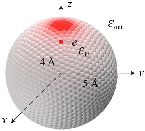
Figure 1: Test system introduced in Ref.51 to examine the accuracy of various Poisson solvers. A positive unit charge is placed 4 Å from the center of a dielectric sphere ($\varepsilon_{\mathrm{in}}=80$) of radius 5 Å. The sphere is embedded in a background medium with relative permittivity $\varepsilon_{\mathrm{out}}=2$. Shading on the sphere surface indicates the induced charge.

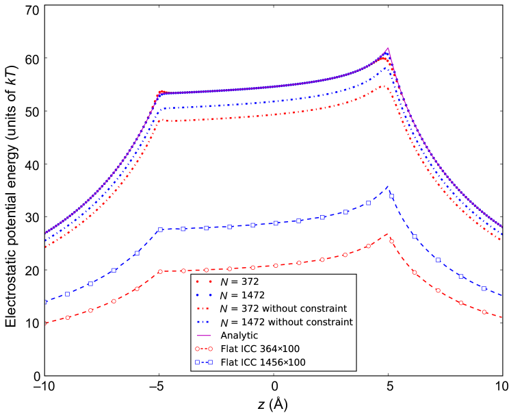
Figure 2: Accuracy comparison between the IDS (iterative dielectric solver) implementation of Ref.31 and more costly alternative techniques for the induced charge potential along the $z$ axis for the configuration of Fig. 1. Purple solid line marks the analytical solution. Open symbols represent data from Ref.52 employing the induced charge computation (ICC) methodBoda et al. (2004), where the sphere is discretized into $364$ (red open circles) and $1456$ (blue open squares) flat patches with $100$ subtiles per patch. The large discrepancy between these data and the analytical result can be significantly reduced by using one-point quadratureBarros, Sinkovits, and Luijten (2014) (dashed lines marked “without constraint,” for comparable patch numbers, namely $372$ (red) and $1472$ (blue)). Enforcing the net induced-charge constraint (cf. Ref.31 and main text) improves the data (small red and blue solid circles) such that they become indistinguishable from the analytical result, except near the two surface boundary points ($z=\pm 5$Å), where discretization effects dominate. This improvement, which is achieved at negligible additional computational cost, can be understood from the eigenvalue spectrum of the operator employed in the IDS (see main text).

In the context of the dielectrically heterogeneous particles examined below, it proves insightful to first closely examine the performance of the IDS approach proposed in Ref.31 for a uniform spherical particle, with specific focus on the consequences of the one-point quadrature in Eqs. (10) and (11). We adopt a test case from Ref.51, i.e., the polarization potential of a dielectric sphere ($\varepsilon_{\mathrm{in}}=80$, $\varepsilon_{\mathrm{out}}=2$) of radius 5 Å, induced by a positive unit charge ($q=+e$) located inside the sphere, at a distance 4 Å away from the sphere center (Fig. 1). In Ref.51, this was found to be a remarkably challenging system, with strong deviations between some numerical approaches and the analytical solution Doerr and Yu (2004) for the induced potential along the $z$-axis. The collocation approach Boda et al. (2004) was observed to yield a potential more than twice smaller than the analytical result for a spherical surface discretized into 364 or 1456 flat tiles, with each tile subdivided into $100$ elements for numerical integration (Fig. 2). On the other hand, the qualocation method Tausch, Wang, and White (2001) was found to yield excellent agreement with the analytical solution for the same tiling and subdivision. Figure 2 shows that even the one-point quadrature implementation of IDS performs far better than collocation with flat disksBoda et al. (2004); Berti et al. (2012), for similar global discretization levels (i.e., number of patches employed for the entire sphere). Yet, the deviation from the analytical result is still quite significant. This is fully mitigated by imposing the “net induced-charge constraint” derived in Ref.31. For this test case, the net induced charge on the sphere is nonzero, and the total (free and bound) charge should be $q/\varepsilon_{\mathrm{out}}$ (Ref.31, Sec. IV.H). The total bound charge itself consists of two contributions: the bound charge at the source charge location ($q/\varepsilon_{\mathrm{in}}-q$) and the surface induced charge, so that the latter must equal $q/\varepsilon_{\mathrm{out}}-q/\varepsilon_{\mathrm{in}}$. To enforce this physical constraint within GMRES, for simplicity we evenly distribute the net charge over all patches for the initial trial solution $\bm{\sigma}^{(0)}$ and enforce the inner product of the patch areas $(a_{1},a_{2},\ldots,a_{N})$ and each subsequent basis vector, $\Delta^{(m)}=\sum_{i=1}^{N}a_{i}(\mathbf{q}_{m})_{i}$, to be zero, by subtracting $\Delta^{(m)}/N$ from the computed induced surface charge of each patch at every iteration. This technique, which comes at negligible computational cost, yields excellent agreement with the analytical solution and rapid convergence as a function of the number of surface patches. Indeed, the accuracy is comparable with the full qualocation approach at similar discretization levels, while avoiding the use of subpatch discretization to obtain the second term of $\mathcal{A}_{ij}$ in Eq. (8) (i.e., only a single evaluation per patch, rather than numerical integration over $100$ subtiles). We note that IDSBarros, Sinkovits, and Luijten (2014) employs patches with a fixed curvature, implemented via a curvature correctionAllen, Hansen, and Melchionna (2001), but this is not to be confused with curved surface elements,Berti et al. (2012) which are computationally far more costly. Also, we have explicitly verified that this curvature correction has a near-negligible effect on the results in Fig. 2.

The high accuracy of IDS for this test case arises from two aspects of the spectrum of the matrix operator $\mathcal{A}$. First, $\mathcal{A}$ is well-conditioned. For $\mathcal{A}\bm{\sigma}=\mathbf{b}$, the $L_{2}$-norm condition number $\kappa(\mathcal{A})=\eta_{\mathrm{max}}(\mathcal{A})/\eta_{\mathrm{min}}(\mathcal{A})$ characterizes the sensitivity of the solution $\bm{\sigma}$ to a perturbation in $\mathbf{b}$, where $\eta_{\mathrm{max}}(\mathcal{A})$ and $\eta_{\mathrm{min}}(\mathcal{A})$ are the largest and smallest singular values of $\mathcal{A}$, respectively. A perturbation $\delta\mathbf{b}$ in $\mathbf{b}$ will lead to a perturbation $\delta\bm{\sigma}$ in $\bm{\sigma}$, whose norm is bounded by the condition number,Higham (2002)

$$\frac{\left\lVert\delta\bm{\sigma}\right\rVert}{\left\lVert\bm{\sigma}\right\rVert}\leq\kappa(\mathcal{A})\frac{\left\lVert\delta\mathbf{b}\right\rVert}{\left\lVert\mathbf{b}\right\rVert}\;.$$ (13)

A typical MD simulation employs a fast Ewald solver with moderate accuracy, leading to inaccuracies in $\mathbf{b}$. Thus, an accurate solution of $\bm{\sigma}$ requires a small condition number $\kappa(\mathcal{A})$. For a normal matrix, $\kappa(\mathcal{A})=|\lambda_{\mathrm{max}}(\mathcal{A})|/|\lambda_{\mathrm{min}}(\mathcal{A})|$, with $\lambda$ its eigenvalues. Whereas the sphere of Fig. 1 is dielectrically isotropic, the patches differ slightly in area, causing the matrix $\mathcal{A}$ to be asymmetric, which results in complex eigenvalues, albeit with small imaginary parts. The condition number $\kappa(\mathcal{A})$ can be computed explicitly, since the spectrum $\lambda$ of $\mathcal{A}$ was solved analytically for a spherical geometry,Barros, Sinkovits, and Luijten (2014)

$$\lambda=\left\{\varepsilon_{\mathrm{out}},\left(\frac{2}{3}\varepsilon_{\mathrm{out}}+\frac{1}{6}\varepsilon_{\mathrm{in}}\right),\ldots,\left(\frac{1}{2}\varepsilon_{\mathrm{out}}+\frac{1}{2}\varepsilon_{\mathrm{in}}\right)\right\}\;.$$ (14)

yielding $\kappa(\mathcal{A})=41/2$, sufficiently small to guarantee a well-conditioned matrix.

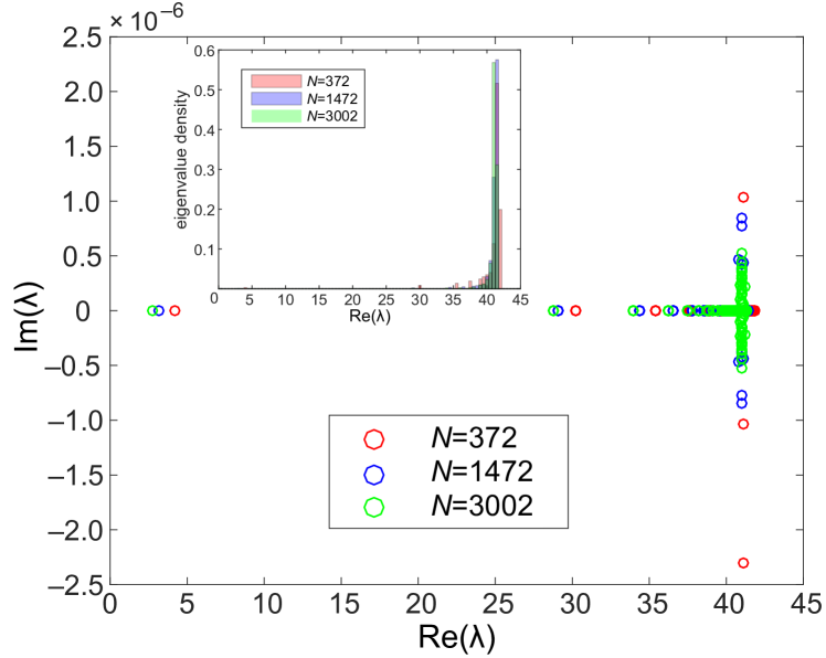
Figure 3: Complex spectrum $\lambda$ of the operator $\mathcal{A}$ in Eq. (10) for the dielectric sphere of Fig. 1 at different discretization levels $N$. As $N$ increases, the real parts of the smallest and largest eigenvalues approach $2$ and $41$, respectively, in agreement with Eq. (14)Barros, Sinkovits, and Luijten (2014). The imaginary parts are small across the entire spectrum, reflecting the near-symmetric character of $\mathcal{A}$. The inset shows the histogram of the real parts $\mathrm{Re}(\lambda)$, illustrating that apart from the outlying smallest eigenvalue all other values are clustered.

In Fig. 3 we evaluate the eigenvalues of $\mathcal{A}$ based upon Eq. (10), at different discretization levels. The extreme eigenvalues $\min(\lambda)$ and $\max(\lambda)$ gradually approach the analytical predictions, i.e., $2$ and $41$, as the patch number $N$ is increased. The relative imaginary parts ${\mathrm{Im}(\lambda)}/{\mathrm{Re}(\lambda)}$ are indeed very small and decrease as $N$ increases, indicating $\mathcal{A}$ is close to a normal matrix. For $372$ patches, we find $\kappa(\mathcal{A})\approx 9.87$.

The second contribution to the accuracy of the IDS also follows from the spectrum. Namely, the convergence rate of GMRES depends on the eigenvalue distribution of $\mathcal{A}$ in the complex plane.Freund, Golub, and Nachtigal (1992) For fast convergence, the eigenvalues should be clustered away from zero, i.e., the distance between any two eigenvalues should be much smaller than the distance of any eigenvalue from the origin.Benzi (2002); Larsen and Morel (2010) Figure 3 shows that the minimum eigenvalue is isolated from the other eigenvalues, compromising the quality of the spectrum. The eigenvector of this outlying eigenvalue is uniform, corresponding to a uniform surface charge density.Barros, Sinkovits, and Luijten (2014) As the total induced charge follows from Gauss’s theorem, this contribution can be computed analytically and imposed as a constraint during the GMRES iterations. Since $\mathcal{A}$ is real and near-symmetric, its eigenvectors are orthogonal. Thus, the physical constraint imposed in the IDS precisely eliminates contributions of the outlying eigenvalue. The remaining eigenvalues are clustered (cf. Fig. 3, inset), ensuring fast convergence of the IDS implementation in Fig. 2. Since each GMRES iteration involves evaluation of the electric field at each patch location subject to the accuracy of the Ewald solver, reduction of the number of iterations reduces the cumulative error as well.

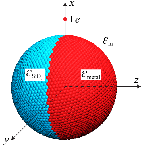
Figure 4: Silica/metal Janus particle of diameter $14\sigma$ (with $\sigma=7.14$ Å). The two hemispheres are separated by a disk-shaped dielectric interface (hidden from view). As a test case of the dielectric solver applied to dielectrically anisotropic particles, we examine the surface potential induced by a positive unit charge located at $(9\sigma,0,0)$.

The IDS, including the net-charge constraint, has been successfully applied to calculate the self-assembly and polarization of suspensions of binary mixtures of isotropic spherical colloids.Barros and Luijten (2014) Indeed, this solver is applicable to arbitrary geometries, but the examination of the dielectric sphere has shown that subtle issues may arise. To clarify these issues in the case of dielectrically heterogeneous particles, where additional dielectric interfaces arise, we consider the prototypical example of a Janus sphere comprised of a silica hemisphere and a metallic hemisphere Wu, Han, and Luijten (2016). This example exhibits three dielectric interfaces: two hemispherical surfaces and one equatorial disk (Fig. 4). The silica side has permittivity $\varepsilon_{\mathrm{SiO_{2}}}=4$ and the permittivity of the conducting side is approximated by $\varepsilon_{\mathrm{h}}=10^{5}$. The system is embedded in an uniform dielectric medium representing water ($\varepsilon_{\mathrm{m}}=80$). We set the diameter of the Janus particle to $d=14\sigma=10$ nm, where $\sigma=7.14$ Å is the Bjerrum length.

To study the accuracy of the IDS, we compute the polarization charge induced on a Janus sphere by a monovalent ion and compare the resulting surface potential to a finite-element calculation performed using the COMSOL package (Version 5.1, 2015). The Janus particle has azimuthal symmetry about the $z$-axis. The positive unit charge is placed $9\sigma$ from its center, at a polar angle $\theta=\pi/2$ (i.e., in the equatorial plane of the Janus particle), so that the external source field acts equally on both hemispheres (Fig. 4). Since the IDS yields the surface charge density rather than the potential, additional errors are introduced when we back-compute the potential on each surface patch, especially for the contributions from immediately neighboring patches and from the patch itself. To reduce such errors we adopt a mesh with 10 242 patches on the sphere and 5 000 patches on the equatorial disk. The electric field is evaluated via PPPM Ewald summation, with a periodic simulation box that is large enough ($400\times 400\times 400\sigma^{3}$) to minimize periodicity artifacts. Both the relative error of the Ewald summation and the convergence criterion of GMRES are set to $10^{-6}$. In the finite-element calculation, a ground potential is imposed at the boundaries of the simulation box. To suppress artifacts resulting from this, we employ the same large simulation cell as for the BEM-based calculation. The entire 3D volume is discretized into a nonuniform mesh with 3 147 897 tetrahedral elements.

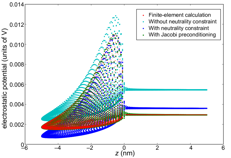
Figure 5: Comparison of different calculations of the total surface potential on a Janus sphere as set up in Fig. 4, i.e., a dielectric Janus particle embedded in water ($\varepsilon_{\mathrm{m}}=80$), with a silica hemisphere ($\varepsilon_{\mathrm{SiO_{2}}}=4$) and a metal hemisphere ($\varepsilon_{\mathrm{h}}=10^{5}$), and a positive unit charge placed at $(9\sigma,0,0)$. The spherical dielectric interface centered at the origin has radius $7\sigma=4.998~{}\mathrm{nm}$ and is divided into 10 242 patches on the sphere and 5 000 patches on the disk that constitutes the metal–silica interface. Red data points represent the surface potential as computed via a FEM calculation. The potential is constant on the metal hemisphere ($z>0$) and varies on the silica hemisphere ($z<0$). Cyan data are obtained with the IDS (iterative BEM-based dielectric solver) without any additional constraints. Blue data are obtained with the same solver, while constraining the net induced charge to zero. Both data sets exhibit significant deviations from the FEM solution. The green data points represent the IDS results obtained with a net-neutrality constraint as well as Jacobi preconditioning of the matrix operator. These results are obtained with negligible additional computational cost compared to a standard solver, and exhibit excellent agreement with the FEM data. See main text for a detailed discussion.

Figure 5 compares the two approaches for the total surface potential. We plot the potential at all patch centroids as a function of their $z$ coordinates. The red symbols show the FEM calculation, with a constant potential on the metal hemisphere ($z>0$). The other symbols all represent BEM calculations using the IDS,Barros, Sinkovits, and Luijten (2014) with different conditions. These data exhibit minor deviations from the constant potential for small positive $z$ (i.e., close to the equatorial plane), caused by discretization. More important, however, are the systematic discrepancies. If no net induced-charge constraint is imposed, the BEM data (cyan) display a strong, systematic deviation from the FEM data. For the metal hemisphere, the surface potential is almost twice higher than the correct result, and also for the silica hemisphere the potential is consistently too high. We emphasize that the data have converged, but to the incorrect result. This behavior is similar to what we observed for the isotropic sphere (Fig. 2), although with significantly larger deviations. Once the net induced-charge constraint is imposed (which amounts to a net-neutrality constraint in this case, as the point charge is located outside the sphere) for the entire Janus particle—i.e., for the entire system comprised of the patches on the two hemispheres as well the patches at the silica–metal interface—these deviations are significantly reduced, but by no means negligible (Fig. 5, blue data). The potential on the metal side is mostly constant, but still too high, and the potential on the silica side only matches the FEM calculation close to the equator.

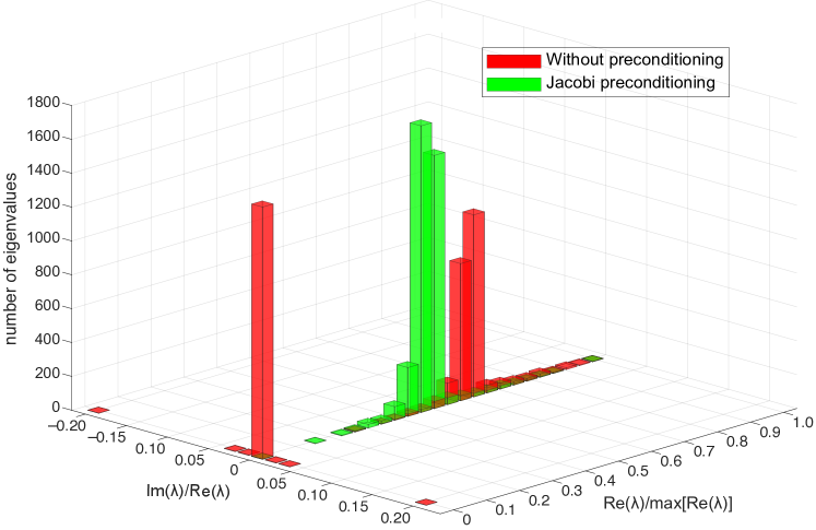
Figure 6: Comparison between the scaled spectra of the matrix $\mathcal{A}$ for a Janus particle (Fig. 4) with Jacobi preconditioning (green data) and without preconditioning (red data). The $x$-axis is scaled by the maximum of the real part of all eigenvalues. The $y$-axis gives the ratio between the imaginary and real parts of each eigenvalue.

To understand and resolve these discrepancies, we again turn to the spectrum of the operator $\mathcal{A}$. We find that the large dielectric mismatches at the metal–water interface and the central metal–silica interface have a detrimental effect on the condition number, yielding $\kappa(\mathcal{A})=2.93\times 10^{3}$. Moreover, as illustrated in Fig. 6 (red data), the spectrum exhibits two groups of normalized eigenvalues, clustered around 0 and 0.65, respectively, resulting in slow convergence. The anisotropy of the Janus particle also results in an asymmetric matrix and significant imaginary parts for some of the eigenvalues, hindering numerical solution of the matrix equation.Saad (1989) To improve this, we apply a preconditioner $\mathcal{M}$ to transform the matrix equation,Benzi (2002) $\mathcal{M}^{-1}\mathcal{A}\bm{\sigma}=\mathcal{M}^{-1}\mathbf{b}$. The choice $\mathcal{M}=\mathcal{A}$ would yield perfect spectral properties, but is prohibitively costly in situations where $\mathcal{A}$ is dynamic. Instead, we observe that the simple Jacobi (or diagonal) preconditioner $\mathcal{M}=\mathrm{diag}(\mathcal{A})=\mathrm{diag}(\bar{\varepsilon}_{ii})$ can be applied here. It is efficient for diagonally dominant matrices,Benzi (2002) as confirmed by the modified spectrum (Fig. 6, green data). With the Jacobi preconditioning, the condition number drops 46-fold to 63.7, and the scaled eigenvalues are clustered around 0.50. These improvements are reflected in the corresponding results for surface potential (Fig. 5, green data), which are in excellent agreement with the FEM calculations. Intuitively, this preconditioning remedies the disproportionate weight of patches with large prefactors in Eq. (10), i.e., large $\bar{\varepsilon}_{i}$ and $\Delta\varepsilon_{i}$ in the residual—precisely the situation that arises if multiple dielectric mismatches are present. This method of preconditioning can be implemented in a particularly simple manner, namely in each iteration of GMRES the residual of the $i$th patch is normalized by $\bar{\varepsilon}_{ii}$.

In summary, these results demonstrate that a combination of high accuracy in the electrostatic summation, a strict convergence criterion in the GMRES method, and a fine discretization level in the BEM are insufficient to guarantee correctness of polarization charge calculations. However, with proper preconditioning to reduce the matrix condition number for systems with multiple dielectric contrasts and a physical (net induced-charge) constraint to eliminate the effects of outlying eigenvalues in the operator spectrum, the iterative dielectric solver of Ref.31 is capable of accurately and efficiently resolving induced charge in systems with multiple dielectric contrasts. A crucial observation is that the preconditioning proposed here can be achieved at no additional computational cost. This is essential for situations where the dielectric environment is time-dependent, such as in dynamical simulations of colloids, proteins, etc., and thus the induced charges must be resolved with the highest possible efficiency. For simplicity, we have focused on the prototypical Janus geometry. However, the techniques presented here to improve the spectrum of the BEM matrix are general and can be applied to a broad variety of dielectric systems.Han, Wu, and Luijten (2016)