Zero-Field Splitting Parameters from Four-Component Relativistic Methods

Abstract

We report an approach for determination of zero-field splitting parameters from four-component relativistic calculations. Our approach involves neither perturbative treatment of spin–orbit interaction nor truncation of the spin–orbit coupled states. We make use of a multi-state implementation of relativistic complete active space perturbation theory (CASPT2), partially contracted $N$-electron valence perturbation theory (NEVPT2), and multi-reference configuration interaction theory (MRCI), all with the fully internally contracted ansatz. A mapping is performed from the Dirac Hamiltonian to the pseudospin Hamiltonian, using correlated energies and the magnetic moment matrix elements of the reference wavefunctions. Direct spin–spin coupling is naturally included through the full 2-electron Breit interaction. Benchmark calculations on chalcogen diatomics and pseudotetrahedral cobalt(II) complexes show accuracy comparable to the commonly used state-interaction with spin–orbit (SI-SO) approach, while tests on a uranium(III) single-ion magnet suggest that for actinide complexes the strengths of our approach through the more robust treatment of spin–orbit effects and the avoidence of state truncation are of greater importance.

I Introduction

The past two decades have witnessed a continuous growth of interest in molecular magnets due to their potential for use in quantum information processing, high-density information storage, and spintronics.Leuenberger and Loss (2001); Bogani and Wernsdorfer (2008); Woodruff et al. (2013) The magnetic properties of open-shell complexes are conventionally modeled using a phenomenological spin Hamiltonian, whose parameters are determined experimentally via electron paramagnetic resonance spectroscopy, magnetometry, inelastic neutron scattering, and other methods.Abragam and Bleaney (1970); Baker et al. (2015); Krzystek and Telser (2016) To second order, the spin Hamiltonian is expressed as

$$\hat{H} =D\left(\hat{S}_{z}^{2}-\frac{1}{3}S(S+1)\right)+E\left(\hat{S}_{x}^{2}-\hat{S}_{y}^{2}\right)+\mu_{B}\mathbf{B}\cdot\mathbf{g}\cdot\hat{\mathbf{S}}$$ (1)

with axial and rhombic zero-field splitting (ZFS) parameters $D$ and $E$, the Bohr magneton $\mu_{B}$, external magnetic field $\mathbf{B}$, the $g$-matrix $\mathbf{g}$ expressing the strength and anisotropy of the electronic Zeeman effect, and spin operator $\hat{\mathbf{S}}$. Additional terms can be added for smaller effects such as hyperfine coupling, interaction with the nuclear quadrupole moment, higher-order ZFS contributions, and so on. One of the key parameters necessary for single-ion magnetism is easy axis ZFS, which contributes to the energy barrier to reversal of spin magnetization. The ZFS is a breaking of degeneracy of the ground spin multiplet of an open-shell complex with total spin of 1 or greater, which results from spin–orbit and spin–spin coupling, and its accurate determination is essential for an understanding of the behavior of molecular magnets.

Several methods are already available for the prediction of spin Hamiltonian parameters. The anisotropic $g$-matrix has been predicted using both relativistic density functional theory and wavefunction-based methods. Malkin et al. (2005); Bolvin (2006); Vancoillie et al. (2007); Neese (2007); Repiský et al. (2010); Chibotaru and Ungur (2012); Ganyushin and Neese (2013); Gohr et al. (2015) For the prediction of zero-field energy splittings, the state-interaction with spin–orbit (SI-SO) approach has been widely used.Ganyushin and Neese (2006) Van den Heuvel et al.Van den Heuvel et al. (2016) have introduced a simplified approach where configuration-averaged Hartree–Fock orbitals are used in a complete active space configuration interaction (CASCI) diagonalization with spin–orbit effects included. This gives comparable results to complete active space self-consistent field (CASSCF) followed by SI-SO for lanthanide systems with weak crystal field effects, although neither method could accurately reproduce the experimental low-energy excitation spectra.Jiang et al. (2010) Contributions from direct spin–spin coupling have been introduced in the context of density functional theory (DFT).Neese (2006)

In this work, we demonstrate a robust method for the ab initio determination of ZFS parameters of mononuclear complexes with strong spin–orbit and spin–spin coupling. Our approach makes use of four-component relativistic CASSCF,Jensen et al. (1996); Bates and Shiozaki (2015); Reynolds et al. (2018) which can be extended with perturbation theory for dynamical correlationShiozaki and Mizukami (2015); Zhang et al. (2018) or the Gaunt or full Breit interactionKelley and Shiozaki (2013) to include direct spin–spin coupling. To extract spin Hamiltonian parameters from the ab initio energies and wavefunctions, we have adapted the pseudospin mapping approach of Chibotaru and UngurChibotaru and Ungur (2012) for the four-component wavefunctions used here.

We begin by reviewing the relevant theory for density fitted, 4-component relativistic CASSCF, fully internally contracted complete active space perturbation theory (CASPT2), and partially contracted $N$-electron valence perturbation theory (NEVPT2). We also review the procedure for mapping to the pseudospin Hamiltonian before going on to benchmark the methods for several series of molecules. We start with a series of chalcogen diatomics, comparing to existing methods and examining the importance of multi-state approaches in each case. We then present example calculations of ZFS parameters for single-ion magnets with moderate and very strong spin–orbit effects. We begin with the pseudotetrahedral cobalt complexes [Co($X$Ph)${}_{4}^{2-}$ for $X$ = O, S, and Se,Zadrozny and Long (2011); Zadrozny et al. (2013); Suturina et al. (2015, 2017), then move on to the actinide complex U(H₂BPz₂)₃,Rinehart et al. (2010); Meihaus et al. (2011); Baldoví et al. (2013); Spivak et al. (2017) where spin–orbit effects are much stronger and should ideally be included concurrently with orbital optimization.

II Theory

II.1 Relativistic CASSCF

Throughout this section, we use $I$, $J$, and $K$ to label Slater determinants, while $L$, $M$, and $N$ refer to CASSCF states. The molecular orbital indices $i$ and $j$ refer to closed orbitals, $r$, $s$, and $t$ to active orbitals, $a$ and $b$ to virtual orbitals; $w$, $x$, $y$, and $z$ are used as generic orbital indices, and $\mu$ is used for atomic basis functions. Our four-component molecular spinors are constructed from a basis set of 2-spinor atomic basis functions generated using restricted kinetic balance (RKB).Stanton and Havriliak (1984); Dyall and Fægri (1990) Starting orbitals are generated from a converged Dirac–Hartree–Fock wavefunction,Kelley and Shiozaki (2013) with active electrons removed when appropriate.

At the level of CASSCF, the multi-configuration wavefunction is parametrized as

$$|M\rangle =\sum_{I}c_{I,M}|I\rangle,$$ (2)

where we seek to find eigenfunctions of the Dirac Hamiltonian within the CASCI space:

$$\langle M|\hat{H}|N\rangle =\delta_{MN}E_{M}.$$ (3)

The relativistic Dirac–Breit Hamiltonian can be expressed in second quantized form as

$$\hat{H}=\sum_{xy}h_{xy}\hat{E}_{xy}+\frac{1}{2}\sum_{xyzw}v_{xy,zw}\hat{E}_{xy_{,}zw}$$ (4)

$$\hat{h}(1)=c^{2}(\beta-I_{4})+c(\bm{\alpha}_{1}\cdot\hat{\mathbf{p}}_{1})-\sum_{A}^{\text{atoms}}\frac{Z_{A}}{r_{1A}}\mathrm{erf}\left(\sqrt{\zeta_{A}}r_{iA}\right)$$ (5)

$$\hat{v}(1,2)=\frac{1}{r_{12}}-\frac{\bm{\alpha}_{1}\cdot\bm{\alpha}_{2}}{r_{12}}-\frac{(\bm{\alpha}_{1}\cdot\bm{\nabla}_{1})(\bm{\alpha}_{2}\cdot\bm{\nabla}_{2})r_{12}}{2},$$ (6)

with the excitation operators defined

$$\hat{E}_{xy}=\hat{a}_{x}^{\dagger}\hat{a}_{y}$$ (7)

$$\hat{E}_{xy,zw}=\hat{a}_{x}^{\dagger}\hat{a}_{z}^{\dagger}\hat{a}_{w}\hat{a}_{y},$$ (8)

and the nuclear potential modeled with a Gaussian charge distribution with exponent $\zeta_{A}$ and total charge $Z_{A}$.Visscher and Dyall (1997) We can also obtain the Dirac–Coulomb–Gaunt or Dirac–Coulomb Hamiltonian by neglecting the last one or two terms (respectively) of Eq. (6).Kelley and Shiozaki (2013)

We perform a two-step optimization procedure to obtain the CASSCF wave functions, where for each macroiteration the state-specific energies are made stationary with respect to $c_{I,M}$ coefficients, i.e.,

$$\frac{\partial E_{M}}{\partial c_{I,M}} =0.$$ (9)

The $c_{I,M}$ coefficients are obtained using the relativistic analogue of full configuration interaction, described previously by one of the authors.Jensen et al. (1996); Bates and Shiozaki (2015) The molecular coefficients are optimized through a series of macroiterations, which makes the state-averaged energy stationary with respect to orbital coefficients $C_{\mu p}$ with appropriate normalizations,

$$\mathbf{C}=\mathrm{exp}(-\bm{\kappa}),$$ (10)

$$\sum_{M}\frac{\partial E_{M}}{\partial\kappa_{pq}}=0.$$ (11)

The orbital optimization is performed using a second-order minimax algorithm, in which explicit construction of the orbital Hessian matrix is avoided by direct multiplication of density fittted integrals to trial vectors; further details are given in Ref. Reynolds et al., 2018.

II.2 Relativistic XMS-CASPT2 and NEVPT2

For the relativistic dynamical correlation theories, we employ a fully internally contracted (FIC) ansatz for the first-order wavefunction, using either the multi-state, multi-reference (MS-MR) parametrization:

$$|\Psi_{M}\rangle=\sum_{N}\hat{T}_{MN}|N\rangle$$ (12)

or the single-state, single-reference (SS-SR) parametrization:

$$|\Psi_{M}\rangle=\hat{T}_{MM}|M\rangle.$$ (13)

The former choice comes at higher cost but ensures the invariance of the correlated wavefunction with respect to rotation among reference states.

For post-CASSCF inclusion of dynamical correlation, we make use of the extended multi-state (XMS) algorithm for quasi-degenerate perturbation theory proposed by Granovsky.Granovsky (2011); Vlaisavljevich and Shiozaki (2016) This is necessary to ensure invariance among rotations between reference states, and can be achieved by diagonalizing the zeroth-order Hamiltonian in the basis of reference states:

$$\sum_{M}\langle L|\hat{H}_{0}|M\rangle U_{MN}=U_{LN}\tilde{E}_{N}$$ (14)

$$|\tilde{M}\rangle=\sum_{N}|N\rangle U_{NM}.$$ (15)

Using the rotated reference functions $|\tilde{M}\rangle$, the implementation of XMS-CASPT2 is the same as conventional MS-CASPT2. There is no need for an extended multi-state algorithm for NEVPT2, because in this case the zeroth-order Hamiltonian is already diagonal.

The zeroth-order Hamiltonian for (X)MS-CASPT2 is given by the state-averaged generalized Fock operator:

$$\hat{H}_{0}^{\text{MS-CASPT2}}=\sum_{M}|M\rangle\langle M|\hat{f}|M\rangle\langle M|+\hat{Q}\hat{f}\hat{Q}+E_{s}$$ (16)

$$\hat{H}_{0}^{\text{XMS-CASPT2}}=\hat{P}\hat{f}\hat{P}+\hat{Q}\hat{f}\hat{Q}+E_{s}$$ (17)

$$\hat{f}=\sum_{xy}f_{xy}\hat{E}_{xy}$$ (18)

$$f_{xy}=h_{xy}+\sum_{zw}d_{zw}^{(0)\text{sa}}\left[(xy|zw)-(xw|zy)\right]$$ (19)

using with a projection to the reference space

$$\hat{P} =\sum_{M}|M\rangle\langle M|$$ (20)

$$\hat{Q} =1-\hat{P}$$ (21)

and state-averaged first-order density matrix

$$d_{zw}^{(0)\text{sa}} =\frac{1}{N_{\mathrm{st}}}\sum_{N}\langle N|\hat{E}_{zw}|N\rangle,$$ (22)

where $N_{\mathrm{st}}$ is the number of states included. $E_{s}$ is a vertical shift parameter.

The working equations for single-state relativistic fully internally contracted CASPT2 and multi-reference configuration interaction (MRCI) were reported by one of us.Shiozaki and Mizukami (2015) The working equations for the residual, source, and norm terms were implemented using the code-generator SMITH3smi and interfaced to the XMS-CASPT2 architecture using the procedure outlined in Ref. Vlaisavljevich and Shiozaki, 2016.

The effective Hamiltonian is constructed including shift corrections for all elements:

$$\begin{split}H_{LL^{\prime}}^{\text{eff}}&=H_{LL^{\prime}}^{\text{ref}}+\frac{1}{2}\sum_{M}\left(\langle\tilde{M}|\hat{T}^{\dagger}_{LM}\hat{H}|\tilde{L}^{\prime}\rangle+\langle\tilde{L}|\hat{H}\hat{T}_{L^{\prime}M}|\tilde{M}\rangle\right)\\ &-E_{s}\sum_{MN}\langle\tilde{M}|\hat{T}^{\dagger}_{LM}\hat{T}_{LN}|\tilde{N}\rangle,\end{split}$$ (23)

the eigenvalues of which correspond to our XMS-CASPT2 second-order energies.

$$\sum_{M}H_{LM}^{\text{eff}}R_{MP} =R_{LP}E_{P}^{MS}$$ (24)

Dyall proposed an alternative formulation of multi-reference perturbation theory, where 2-electron interactions among active orbitals are fully included in the zeroth-order Hamiltonian, which he called the CAS/$A$ operator.Dyall (1995)

$$\hat{H}_{0}^{\text{CAS/$A$}} =\hat{P}\hat{f}^{(A)}\hat{P}+\hat{Q}\hat{f}^{(A)}\hat{Q}+E_{s}$$ (25)

$$\begin{split}\hat{f}^{(A)}&=\sum_{xy}f_{xy}\hat{E}_{xy}-\sum_{rs}f_{rs}\hat{E}_{rs}\\ &+\sum_{rs}h_{rs}\hat{E}_{rs}+\frac{1}{2}\sum_{rs,xy}v_{rs,xy}\hat{E}_{rs,xy}\end{split}$$ (26)

Using only the diagonal blocks of Dyall’s zeroth-order Hamiltonian allows us to run partially contracted NEVPT2.Angeli et al. (2001, 2002)

$$\hat{H}_{0}^{\text{NEVPT2}} =\hat{P}\hat{f}^{(A_{D})}\hat{P}+\hat{Q}\hat{f}^{(A_{D})}\hat{Q}+E_{s}$$ (27)

$$\begin{split}\hat{f}^{(A_{D})}&=\sum_{ij}f_{ij}\hat{E}_{ij}+\sum_{ab}f_{ab}\hat{E}_{ab}\\ &+\sum_{rs}h_{rs}\hat{E}_{rs}+\frac{1}{2}\sum_{rs,xy}v_{rs,xy}\hat{E}_{rs,xy}\end{split}$$ (28)

II.3 Mapping to Pseudospin Hamiltonian

For complexes with spin larger than 1, the energies alone are insufficient to define the ZFS parameters, so the ab initio states must be mapped to a model Hamiltonian.Maurice et al. (2009); Chibotaru and Ungur (2012) In order to determine the spin Hamiltonian parameters, we require a mapping from the eigenfunctions of the Hamiltonian to a suitable basis of effective or fictitious spin states. We first compute the matrix elements of the magnetic moment operator

$$\hat{\bm{\mu}} =-\mu_{B}\sum_{j}\left[\frac{1}{2}g_{e}\hat{\bm{\Sigma}}_{j}-i\mathbf{r}_{j}\times\bm{\nabla}_{j}\right]$$ (29)

using the four-component analogue of the Pauli spin operator,

$$\hat{\bm{\Sigma}} =\begin{pmatrix}\bm{\sigma}&0\\ 0&\bm{\sigma}\end{pmatrix},$$ (30)

where $\bm{\sigma}$ contains the three standard 2-component Pauli spin matrices.Bauke et al. (2014) We build the matrix representation of $\hat{\mu}_{z^{\prime}}$ within the selected manifold of states and diagonalize it. By convention, $z^{\prime}$ is chosen to be one of the main magnetic axes of the complex, which can be determined as described by Chibotaru and Ungur.Chibotaru and Ungur (2012); Chibotaru (2013)

The column eigenvectors of $\bm{\mu}_{z^{\prime}}$ give us the appropriate combinations of Hamiltonian eigenfunctions that should be put in correspondence of pseudospin eigenfunctions, with one complication. The phases of the column eigenvectors are arbitrary, while certain phase restrictions on the pseudospin eigenfunctions must be enforced. The first requirement is time-reversal symmetry, the restoration of which is considered in the Supporting Information. Apart from time-reversal symmetry, the relative phase between pseudospin eigenfunctions is in principle arbitrary; however, we must ensure that the relative phase of true angular momentum matrix elements matches that of the pseudospin operators. The conventional choice is that which makes the Clebsch–Gordon coefficients real;Cohen-Tannoudji et al. (1977) it can be enforced in our context by choosing a phase transformation such that all the $\langle m_{s}|\hat{\mu}_{x^{\prime}}|m_{s}+1\rangle$ matrix elements are real and positive. This requirement ensures that the pseudospin reduces to the true spin $\hat{\mathbf{S}}$ at the limit of zero spin–orbit and spin–spin coupling and leads to consistent behavior under rotation of the coordinate system.

II.4 Extracting the Zero-Field Splitting Parameters

The numerical pseudospin Hamiltonian is constructed from eigenstates of the ab initio Hamiltonian.

$$\left(H_{\mathrm{diag}}\right)_{ij}=\delta_{ij}E_{i}$$ (31)

$$\mathbf{H}_{\mathrm{ZFS}}=\mathbf{U}^{\prime-1}\mathbf{H}_{\mathrm{diag}}\mathbf{U}^{\prime}$$ (32)

where $E_{i}$ is the energy of state $i$, and $\mathbf{U}^{\prime}$ contains the phase-adjusted eigenvectors of $\mu_{z^{\prime}}$ as discussed above and further in the Supporting Information. When the pseudospin Hamiltonian is built up in terms of extended Stevens operators, we have in matrix form

$$\mathbf{H}_{\mathrm{ZFS}} =\sum_{kq}B_{k}^{q}\mathbf{O}_{k}^{q}.$$ (33)

The extended Stevens operators are built from pseudospin operators; for ZFS, the nonzero contributions will have even $k$ between $2$ and $2\tilde{S}$, while $q$ runs from $-k$ to $k$. The general algorithm for generation of the extended Stevens operators has been published by RyabovRyabov (1999, 2009) and is concisely recapitulated in the Supporting Information.

Setting Eqs. (32) and (33) equal leads to a set of linear equations for the coefficients $B_{k}^{q}$. The second-order contributions are more often expressed in terms of the $D$-tensor

$$\mathbf{H}_{\mathrm{ZFS}}^{(2)} =\sum_{q}B_{2}^{q}\mathbf{O}_{2}^{q}=\tilde{\mathbf{S}}\cdot\mathbf{D}\cdot\tilde{\mathbf{S}},$$ (34)

with the parameters

$$\begin{split}&D_{xx}=-B_{2}^{0}+B_{2}^{2}\\ &D_{zz}=2B_{2}^{0}\\ &D_{zx}=D_{xz}=\frac{1}{2}B_{2}^{1}\end{split}\begin{split}&D_{yy}=-B_{2}^{0}-B_{2}^{2}\\ &D_{xy}=D_{yx}=B_{2}^{-2}\\ &D_{yz}=D_{zy}=\frac{1}{2}B_{2}^{-1}\end{split}$$ (35)

and the conventional $D$ and $E$ parameters derived from the diagonalized form of $\mathbf{D}$.

For dynamically correlated calculations, we approximate the mapping to pseudospin states by using rotated reference CASSCF reference functions to determine the magnetic moment matrices,

$$\bm{\mu}_{PQ} =\sum_{MN}\langle\tilde{M}|\hat{\bm{\mu}}|\tilde{N}\rangle R_{MP}^{\ast}R_{NQ}.$$ (36)

Using these matrices, the transformation matrix $\mathbf{U}^{\prime}$ is determined as normal, but the dynamically correlated energies are used when building the Hamiltonian in Eq. (31). In this way, we capture the effects of correlation on energy splittings as well as any mixing that occurs in (extended) multi-state methods, while avoiding the computation of relaxed density matrices associated with the dynamically correlated methods. We consider this approach similar in spirit to the common practice with state interaction methods of using correlated energies along only the diagonal elements of the spin–orbit Hamiltonian.Malmqvist et al. (2002)

III Computational Details

Four-component relativistic calculations were performed with the BAGEL electronic structure packagebag ; Shiozaki (2018) developed by our group. We use spinor basis functions and make use of density fitting with a customized fitting basis set described below. Except where otherwise noted, the Dirac–Coulomb relativistic Hamiltonian was used. Reference data using the SI-SO approach were computed in MOLCASAquilante et al. (2016) and made use of density fitting with an atomic compact fitting basis setAquilante et al. (2007) generated on the fly.

There is some difficulty in the use of contracted orbital basis sets with four-component relativistic calculations. Part of the basis set incompleteness error stems from the fact that convetional basis sets are optimized using a different Hamiltonian operator, but there are additional complications due to restricted kinetic balance. Because the RKB condition does not exactly reproduce the relationship between large and small components in the presence of relativistic effects, a strongly contracted basis function optimized for the large component will generate a small component basis function that is not optimal.Visscher et al. (1991) Dyall has made some effort to develop basis sets for fully relativistic calculations with different contractions for each of the four components.Dyall (1998, 2004, 2006); Dyall and Gomes (2010) Currently, our program can only accommodate one set of contraction coefficients in accord with the RKB condition, and in our previous work we found Dyall’s spin-free basis sets to be inadequate for our needs.Reynolds and Shiozaki (2015) The safest approach is to fully decontract the basis set, but many calculations would be intractable with the large primitive basis sets that result.

In this work, the Atomic Natural Orbitals - Relativistically Core Correlated (ANO-RCC) basis setsRoos et al. (2005) are used for all atoms. In Section IV.1, results for a series of small molecules are given for both the uncontracted form and the triple-$\zeta$ plus polarization (TZP) contraction of this basis set. For four-component calculations on the larger molecules studied in this work, we compromise by using an uncontracted basis on the central metal atom and contracted basis sets on the ligands, with the set of contractions specified in the appropriate section. For the SI-SO comparison data, the TZP contraction is used for central metal atoms, because the atomic mean field integrals used in the SI-SO cannot be accurately computed with a primitive basis set in MOLCAS.Ungur (2016)

We require a customized auxiliary basis set for density fitting because standard fitting basis sets do not include heavy atoms or contain the flexibility needed to capture the Gaunt for full Breit interaction.Kelley and Shiozaki (2013) To meet these demands, we have augmented standard basis sets in an even-tempered manner by adding primitive functions with Gaussian exponents increasing by a factor of 2.5. For H atoms we have simply decontracted the standard TZVPP-JKFIT auxiliary basis set. For B, C, N, O, S, Co, and Se, we have decontracted the TZVPP-JKFIT auxiliary basis set, and we added one tight function to each of the $p$, $d$, and $f$ shells. For Te and U, we begin with the decontracted ANO-RCC basis set. We add polarization functions by applying the exponents of the highest angular momentum functions to higher shells up to $i$-type (i.e., for Te the exponents of 3 $g$ functions are copied to the $h$ and $i$ shells, and for U the 3 $h$ exponents are copied to $i$). We then add several tight functions to each shell, with each one’s exponent greater than the last by a factor of 2.5. The numbers of functions added are as follows: 3 $s$, 3 $p$, 6 $d$, 7 $f$, 5 $g$, and 1 $h$ for Te, and 4 $s$, 4 $p$, 7 $d$, 8 $f$, 6 $g$, 6 $h$, and 5 $i$ for U.

For dynamically correlated calculations, core orbitals were frozen to reduce the cost of the calculation. In some cases, the higher-energy virtual orbitals resulting from basis set decontraction were deleted as well; the energy cutoffs are specified in the relevant results section. A vertical shift of 0.2 was used in four-component XMS-CASPT2 and NEVPT2 calculations, with correction terms included in all elements of the effective Hamiltonian.Roos and Andersson (1995); Vlaisavljevich and Shiozaki (2016) For CASPT2 + SI-SO, an imaginary shift of 0.2 was used along with the standard 0.25 IPEA shift.Forsberg and Malmqvist (1997); Ghigo et al. (2004)

All computations were performed at the experimental structures.Huber and Herzberg (1979); Rinehart et al. (2010); Zadrozny et al. (2013); Suturina et al. (2017) The bond lengths (for diatomics) and molecular coordinates (for larger molecules) are provided in the Supporting Information. For the larger molecules, heavy atom positions were obtained from the crystal structure, and hydrogen positions were optimized using DFT. The DFT optimizations were performed using the Turbomole package.Ahlrichs et al. (1989); Furche et al. (2014) We used the PBE functionalPerdew et al. (1996) along with the def2-TZVPP basis set for all atoms except U, for which we used def-TZVPP with effective core potential.Weigend et al. (1998); Weigend and Ahlrichs (2005); Dolg et al. (1989); Küchle et al. (1994); Cao et al. (2003) We also used the resolution of the identity approximation along with the corresponding RI-J auxiliary basis sets.Eichkorn et al. (1997); Weigend (2006)

IV Results and Discussion

IV.1 Benchmarking Dynamical Correlation Methods with Chalcogen Diatomics

Table 1: Axial ZFS ($D$) of chalcogen diatomics computed with various methods for an active space of 8 electrons in 6 orbitals. Rhombic splitting ($E$) is zero by symmetry.

Molecule		O2			S2			Se2			Te2
States		Triplet	6 lowest		Triplet	6 lowest		Triplet	6 lowest		Triplet	6 lowest
TZP contraction of ANO-RCC
CASSCF		$3.8$	$3.0$		$24.4$	$19.9$		$505.6$	$434.5$		$2067.4$	$1896.0$
XMS-CASPT2		$1.0$	$2.7$		$8.2$	$19.7$		$234.4$	$412.6$		$1428.6$	$1913.8$
NEVPT2		$2.7$	$2.9$		$20.1$	$20.0$		$424.3$	$422.5$		$1931.3$	$1952.1$
MRCI+Q		$2.7$	$2.9$		$22.5$	$20.7$		$470.9$	$440.6$		$2052.4$	$1955.6$
Decontracted ANO-RCC
CASSCF		$3.8$	$3.0$		$27.9$	$22.7$		$558.7$	$480.3$		$2088.6$	$1905.9$
XMS-CASPT2		$1.1$	$2.9$		$9.9$	$23.9$		$278.6$	$489.7$		$1401.1^{,}$	$1944.3^{,}$
NEVPT2		$2.9$	$3.0$		$24.0$	$24.5$		$497.0$	$502.7$		$1957.1^{,}$	$1994.8^{,}$
Experiment		4.0			23.5			510.0			1975.0

Table 1 presents ZFS results for a series of chalcogen diatomics using the methods reported in the previous sections. The diatomics in this series have been previously used to benchmark other methods by Rota et al.Rota et al. (2011) For dynamically correlated calculations, deep core orbitals were frozen (2 for S₂, 10 for Se₂, and 18 for Te₂). As indicated in the table, an additional 18 semi-core orbitals were frozen in some Te₂ calculations to reduce the cost. These benchmark tests were performed with the MS-MR parametrization.

We have also tested the influence of basis set contraction upon ZFS results, because ANO-RCC basis contractions are not optimized for the four-component treatment of relativistic effects. Due to cost constraints, MRCI+Q results are included only for the contracted basis set, and in some cases high-energy virtual orbitals were deleted. In most cases, the results with the contracted basis set are further from the experimental values, with errors of 10–20% in the cases of S₂ and Se₂, and smaller errors for O₂ and Te₂. This suggests that in the pursuit of high-quality results without the large costs associated with decontraction, there is use for further development of basis sets suitable for four-component relativistic calculations. For the time being, we prefer using uncontracted basis sets and compromise when necessary by contracting basis sets on ligands but not spin centers.

The XMS-CASPT2 results in Table 1 show an extremely strong dependence upon the choice of states to include in the calculation, with large errors introduced when excluding some low-lying excited singlets. The choice of which excited states to include affects the calculation primarily in two ways: through the orbital optimization in state-averaged CASSCF, and through the zeroth-order Hamiltonian which uses a state-averaged density matrix. Table S2 in the Supporting Information separates these effects by correlating the first three or six states using both sets of orbitals, and clearly shows that the zeroth-order Hamiltonian is the main source of error; the change to the state-averaged orbitals alters the XMS-CASPT2 splitting by a few percent only. It is unsurprising, then, that the strong dependence on state averaging is not observed in the other methods; Dyall’s Hamiltonian used by NEVPT2 replaces the active-active part of the state-averaged Fock matrix with the full Hamiltonian, and MRCI+Q does not use it at all.

MRCI+Q is unsurprisingly the most reliable method tested here, although for large problems it will be intractable. When a more approximate dynamically correlated method is needed, NEVPT2 is preferred due to its relatively low sensitivity to the set of states included, although for this series the accuracy of CASSCF is competitive with the perturbative methods, in comparison to experimental values.

We briefly mention one other complication which has been observed. For calculations with a very minimal active space (e.g., 2 electrons in 2 orbitals with all six states included), it is possible for states which are nondegenerate under $\hat{H}$ to become degenerate under $\hat{H}_{0}$ and, therefore, to freely mix in the XMS rotation. In such cases, if a vertical shift is used with only the diagonal correction terms, unphysical breaking of Kramers degeneracy will result, but if no shift is used or we correct the entire effective Hamiltonian, degeneracy is restored in the final multi-state mixing step.

IV.2 Zero-Field Splitting of Pseudotetrahedral Cobalt(II) $(\bm{X}$Ph$)_{\bm{4}}$ Complexes

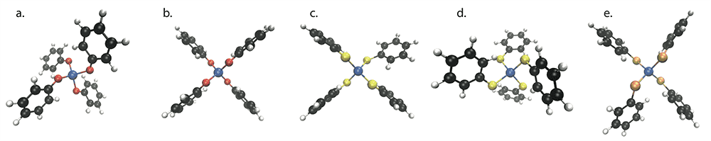
Figure 1: Geometry of the Co$(X$Ph$)_{4}$ complexes tested. (a.) Co(OPh)${}_{4}^{2-}$ crystallized with 2 PPh${}_{4}^{+}$ and 2 CH₃CN.Zadrozny et al. (2013) (b.) Co(OPh)${}_{4}^{2-}$ crystallized with PPh${}_{4}^{+}$ and K⁺.Zadrozny et al. (2013) (c.) Co(SPh)${}_{4}^{2-}$ crystallized with 2 PPh${}_{4}^{+}$.Suturina et al. (2017) (d.) Co(SPh)${}_{4}^{2-}$ crystallized with 2 N(CH₂CH${}_{3})_{4}^{+}$.Suturina et al. (2017) (e.) Co(SePh)${}_{4}^{2-}$ crystallized with 2 PPh${}_{4}^{+}$.Zadrozny et al. (2013)

To gauge the performance of relativistic correlation methods for mononuclear transition metal complexes, we look to the series of pseudotetrahedral cobalt(II) $(X$Ph$)_{4}$ complexes with $X$ = O, S, Se whose structures are shown in Figure 1. Molecule (c), (PPh₄)₂Co(SPh)₄ was one of the first field-free transition metal single-ion magnets to be discovered;Zadrozny and Long (2011) the analogous complexes here have been characterized both experimentally and theoretically to probe the magneto-structural correlations present.Zadrozny et al. (2013); Suturina et al. (2015, 2017) Structures (a) and (b) as well as (c) and (d) differ only in the counter ion and solvent present in the crystal, which dramatically alters both the conformation and ZFS of the anion.

CASSCF-level ZFS parameters computed for the whole series are compared along with experimental values in Table 2. A mixed basis set is used, with the central cobalt atom decontracted in four-component results, the TZP contraction for chalcogen atoms, the double-$\zeta$ plus polarization (DZP) contraction for carbon atoms, and double-$\zeta$ (DZ) for hydrogen atoms. Agreement with experiment is reasonably good for this series, with qualitative agreement throughout. The major exception is the Dirac-CASSCF results with only the ground quartet included in the state-averaging procedure; in most cases more accurate results are obtained when the orbitals are balanced by including all $d^{5}$ excitations (10 quartets and 40 doublets). The choice of whether to include a second, correlating set of $d$-orbitals is of lesser importance, typically altering the observed splitting by a few wavenumbers or less.

Table 2: ZFS of the pseudotetrahedral cobalt(II) $(X$Ph$)_{4}$ series at the CASSCF level of theory. Energies are given in cm^-1. Calculations are based on an active space of 7 electrons in either 5 or 10 active $d$-orbitals.

Molecule	Active Space	Dirac Ham.		Dirac Ham.		Scalar + SI-SO		Experiment
		ground quartet		full $d^{5}$		(full $d^{5}$)
	7 e-, 5 orb.	$D=$	$-9.5$	$D=$	$-13.6$	$D=$	$-13.5$
Co(OPh)${}_{4}^{2-}$		$E=$	$1.4$	$E=$	$2.1$	$E=$	$2.1$	$D=-11.1(3)$
Geometry (a)	7 e-, 10 orb.	$D=$	$-10.1$	$D=$	$-13.5$	$D=$	$-12.6$	$(E=0.0)$
		$E=$	$1.4$	$E=$	$1.9$	$E=$	$1.8$
	7 e-, 5 orb.	$D=$	$-15.1$	$D=$	$-24.6$	$D=$	$-24.5$
Co(OPh)${}_{4}^{2-}$		$E=$	$0.0$	$E=$	$0.0$	$E=$	$0.0$	$D=-23.8(2)$
Geometry (b)	7 e-, 10 orb.	$D=$	$-16.2$	$D=$	$-22.5$	$D=$	$-22.5$	$(E=0.0)$
		$E=$	$0.0$	$E=$	$0.0$	$E=$	$0.0$
	7 e-, 5 orb.	$D=$	$-31.1$	$D=$	$-58.3$	$D=$	$-58.3$
Co(SPh)${}_{4}^{2-}$		$E=$	$1.6$	$E=$	$1.6$	$E=$	$1.6$	$D=-62(1),-55(1)$
Geometry (c)	7 e-, 10 orb.	$D=$	$-36.2$	$D=$	$-58.0$	$D=$	$-58.0$	$E=0(2)$
		$E=$	$1.7$	$E=$	$1.5$	$E=$	$1.5$
	7 e-, 5 orb.	$D=$	$10.9$	$D=$	$16.9$	$D=$	$16.9$
Co(SPh)${}_{4}^{2-}$		$E=$	$1.7$	$E=$	$2.5$	$E=$	$2.5$	$D=11(2)$
Geometry (d)	7 e-, 10 orb.	$D=$	$11.9$	$D=$	$15.3$	$D=$	$15.3$	$E=2.0(4)$
		$E=$	$1.8$	$E=$	$2.3$	$E=$	$2.3$
	7 e-, 5 orb.	$D=$	$-38.7$	$D=$	$-80.4$	$D=$	$-80.4$
Co(SePh)${}_{4}^{2-}$		$E=$	$1.5$	$E=$	$1.2$	$E=$	$1.2$	$D=-83(1)$
Geometry (e)	7 e-, 10 orb.	$D=$	$-45.3$	$D=$	$-80.3$	$D=$	$-80.3$	$(E=0.0)$
		$E=$	$1.7$	$E=$	$1.0$	$E=$	$1.0$

Four-component NEVPT2 calculations have also been performed on structures (a), (c), and (e) of this series; the results are summarized in Table 3. Due to cost constraints, it was necessary to reduce the basis set combination used: for these data, the basis sets for cobalt and hydrogen are the same as above, but the DZP contraction was used for chalcogen atoms and the DZ contraction for carbon atoms. All results in this table use an active space of 7 electrons in 5 active orbitals. For Dirac-NEVPT2, the MS-MR contraction is used while correlating the four lowest states, but using orbitals that were obtained by finding a minimax state-averaged energy for all excitations of $d$-electrons. The number of frozen core orbitals is 37, 53, and 69 for structures (a), (c), and (e), respectively. 89 high-energy virtual orbitals were deleted, corresponding to an energy cutoff threshold of 11 $E_{\mathrm{h}}$ to avoid splitting up near-degenerate orbitals at 10 $E_{\mathrm{h}}$.

We used the MS-MR internal contraction scheme in this and the previous section. It is tempting to switch to the SS-SR parametrization, which would reduce the memory cost by roughly a factor of $N_{\mathrm{st}}$ and the timing cost by a greater amount. Some tests have been performed using truncated models for this molecular series; the details are presented in the Supporting Information. We found that reducing the expansion set to the SS-SR scheme introduced errors in the splitting energies of several percent, and that the ratio $|E/D|$ was much more sensitive. Therefore, we prefer the MS-MR parametrization when possible, while noting that the errors introduced by SS-SR in the energy spacings were moderate.

We see corrections due to dynamical correlation of 2 to 20 cm^-1, slightly larger than are observed in the CASPT2 + SI-SO reference data. The basis set reduction necessary to make the NEVPT2 calculations tractable introduced errors of up to 3.6 cm^-1 at the Dirac-CASSCF level, showing somewhat higher basis set sensitivity than the SI-SO results; one might expect a somewhat greater basis set incompleteness error in the correlated data, which would be consistent with the results in Table 1 for smaller test systems. For structure (a), the Dirac-NEVPT2 best reproduces the experimental findings, but for the other two complexes it appears to overcorrect.

Table 3: ZFS for a subset of the pseudotetrahedral cobalt(II) $(X$Ph$)_{4}$ series. Energies are given in cm^-1. Calculations are based on an active space of 7 electrons in 5 active $d$-orbitals and with a smaller basis set than in Table 2, as discussed in the main text.

Molecule	CASSCF				NEVPT2		CASPT2		Experiment
	Dirac Ham.		Scalar + SI-SO		Dirac Ham.		Scalar + SI-SO
Co(OPh)${}_{4}^{2-}$ (a)	$D=$	$-13.9$	$D=$	$-13.9$	$D=$	$-11.3$	$D=$	$-13.1$	$D=-11.1(3)$
	$E=$	$2.1$	$E=$	$2.1$	$E=$	$1.5$	$E=$	$1.7$	($E=0.0$)
Co(SPh)${}_{4}^{2-}$ (c)	$D=$	$-61.9$	$D=$	$-58.8$	$D=$	$-43.3$	$D=$	$-53.1$	$D=-62(1),-55(1)$
	$E=$	$1.6$	$E=$	$1.6$	$E=$	$1.5$	$E=$	$1.1$	$E=0(2)$
Co(SePh)${}_{4}^{2-}$ (e)	$D=$	$-83.1$	$D=$	$-80.9$	$D=$	$-63.8$	$D=$	$-72.4$	$D=-83(1)$
	$E=$	$1.2$	$E=$	$1.0$	$E=$	$1.3$	$E=$	$0.7$	($E=0.0)$

IV.3 Zero-Field Splitting of a Uranium(III) Pyrazole Complex

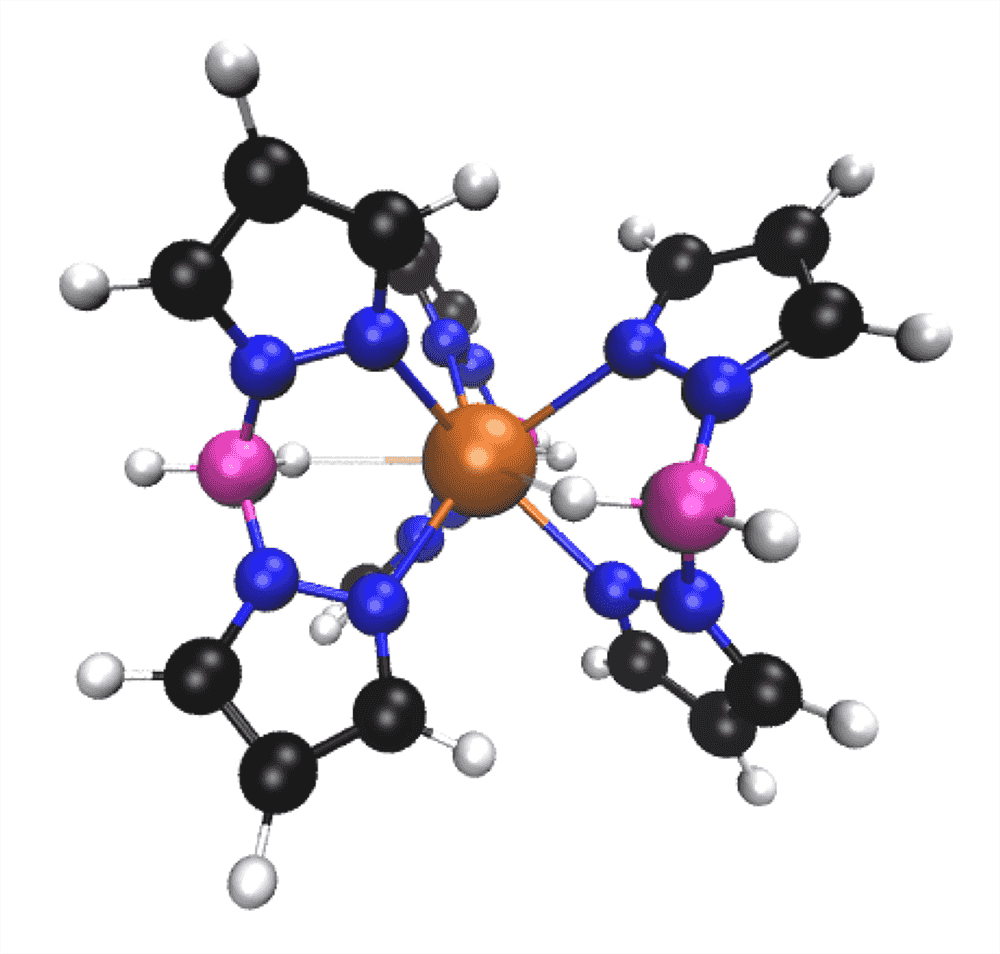
Figure 2: Geometry of U(H₂BPz₂)₃.Rinehart et al. (2010)

To test the performance of these methods for magnetic complexes with very heavy elements, we have computed the ZFS of the ground $J=\tfrac{9}{2}$ multiplet in the uranium(III) dihydrobispyrazolylborate complex U(H₂BPz₂)₃, shown by Long and co-workers to act as a single-ion magnet in magnetically dilute samples.Rinehart et al. (2010); Meihaus et al. (2011) The structure is depicted in Figure 2, and results are presented in Table 4. Previous theoretical calculations have been carried out with the SI-SO approach by Spivak et al.Spivak et al. (2017) and with a semi-empirical crystal-field approach by Baldovi et al.Baldoví et al. (2013) The results reported by Spivak et al. show a somewhat smaller splitting than that in Table 4, which might result from a different choice of molecular geometry; further details are discussed in the Supporting Information.

The results in Table 4 were computed with either the decontracted basis or TZP contraction for the uranium atom as appropriate, the DZP basis set for boron, carbon, and nitrogen atoms, and the DZ contraction for hydrogen atoms. An exception is the Dirac-NEVPT2 result, for which the polarization functions were not used for main group elements; one column also shows CASSCF results with the same basis set. The active space in all cases is 3 active electrons in the 7 $f$-orbitals. Orbital optimizations were perfomed for the minimax state-averaged energy for all excitations within the $f$-orbitals. NEVPT2 calculations included the lowest 10 states and used the SS-SR parametrization; 72 core orbitals were frozen, and 160 virtual orbitals were deleted, corresponding to an energy cutoff of 10 $E_{\mathrm{h}}$.

We computed an excitation energy of 161.2 cm^-1 with Dirac-CASSCF and 103.3 cm^-1 with NEVPT2, somewhat lower than the value of 230 cm^-1 predicted by a semi-empirical crystal-field approach.Baldoví et al. (2013) We obtain qualitatively similar results with Dirac-CASSCF vs. CASSCF + SI-SO. The Breit correction at the CASSCF level was determined to be only a few wavenumbers, smaller than other errors relating to electron correlation and the molecular geometry dependence.

The excitation spectrum of U(H₂BPz₂)₃ is not available for comparison. The closest analogue we have is a measurement of the magnetic relaxation barrier, which was found to be 16 cm^-1 in a magnetically dilute sample.Meihaus et al. (2011) All theoretical methods examined here give a first excited state at least several times higher. There are several competing relaxation mechanisms in this molecule,Meihaus et al. (2011) so the observed barrier is not directly related to the energy splitting computed in this work.

The CASPT2 + SI-SO approach requires computing the second-order correlation energy for a large number of excited states, and there are practical limits to how many states can be included. We have truncated our CASPT2 space at 21 quartets and 11 doublets, out of 35 quartets and 112 doublets accessible by exciting within the $f$-orbital manifold, which is the same cutoff used in the earlier study.Spivak et al. (2017) As shown in Table 4, truncating the coupling of CASSCF states at the same level shifts the energy splittings by 70-160 cm^-1, so the aggressive truncation needed for large active spaces comes at a substantial accuracy cost for ZFS calculations. One of the advantages of the four-component approach is that spin–orbit effects are included from the start and can be captured without computing many excited states, so it avoids this particular problem. Of course, there is a tradeoff; the large memory costs associated with the four-component NEVPT2 required us to make compromises to limit the number of orbitals included in the correlation, although in this case the errors associated with reducing the basis set are manageable, at least at the CASSCF-level. For this molecule, the Dirac-NEVPT2 correction to the enery splittings is of comparable magnitude but opposite sign relative to the CASPT2 + SI-SO reference.

Table 4: Low-lying energy spectrum of U(H₂BPz₂)₃. Energies are given in cm^-1. Calculations are based on an active space of 3 electrons in the 7 active $f$-orbitals.

Eigenstates	Dirac Hamiltonian				State-interaction with Spin-Orbit			Crystal field
	CASSCF	Breit corr.	CASSCF	NEVPT2	CASSCF (full)	CASSCF (trunc.)	CASPT2 (trunc.)	Semi-empirical
States 1 - 2	$0.0$	$0.0$	$0.0$	$0.0$	$0.0$	$0.0$	$0.0$	$0$
States 3 - 4	$161.2$	$1.3$	$163.3$	$103.3$	$165.4$	$96.4$	$154.2$	$231$
States 5 - 6	$407.5$	$-2.3$	$412.3$	$425.4$	$406.9$	$286.8$	$275.0$	$491$
States 7 - 8	$524.1$	$0.2$	$525.0$	$503.9$	$511.4$	$392.3$	$397.9$	$609$
States 9 - 10	$644.4$	$2.8$	$651.0$	$570.1$	$611.2$	$452.0$	$482.4$	$842$

V Conclusions

We have developed a computational tool for the determination of ZFS parameters in relatively large molecules containing strong relativistic effects. Specifically, we report the development of (extended) multistate implementations of four-component relativistic CASPT2, NEVPT2, and MRCI as well as a mapping from the four-component wavefunctions to a pseudospin Hamiltonian for the extraction of ZFS parameters. We observed a surprisingly large dependence upon the state-averaging procedure used to obtain the orbitals, which is troublesome for XMS-CASPT2 but reduced in CASSCF, NEVPT2, and MRCI+Q. Benchmark calculations performed on the series of chalcogen diatomics and pseudotetrahedral Co$(X$Ph$)_{4}$ complexes showed similar results to the less costly scalar relativistic + SI-SO approach, suggesting that for light elements the fully relativistic methods can serve as a useful benchmark but are not always needed. Tests on the actinide single-molecule magnet U(H₂BPz₂)₃ showed larger effects, indicating that for very heavy metals the simultaneous treatment of relativity and electron correlation, as well as avoidance of state truncation sometimes required for SI-SO, can be helpful when attempting high-accuracy calculations. The methods reported in this manuscript are publicly available in the BAGEL program packagebag and distributed under the GNU General Public License.

VI Associated Content

VI.1 Supporting Information

The following content is available in the Supporting Information: Discussion of the theory and working equations used in the implementation of the mapping to the pseudospin Hamiltonian; ZFS results for chalcogen diatomics with a reduced active space, including an investigation to separate the effects of state-averaged orbitals and state-averaged Fock operator on dynamically correlated results; comparison of ZFS results using the SS-SR and MS-MR parametrizations for truncated models of the Co($X$Ph)${}_{4}^{2-}$ series; discussion of the molecular geometry of U(H₂BPz₂)₃ and the effects of optimization of hydrogen positions; xyz coordinates of the molecules used for testing.

VII Acknowledgments

The authors thank Scott Coste and Danna Freedman for helpful discussions. RDR has been supported by the DOD National Defense Science and Engineering Graduate (NDSEG) Fellowship, 32 CFR 168a. TS has been supported by the NSF CAREER Award (CHE-1351598). TS is an Alfred P. Sloan Research Fellow. Some of the computations were performed with the aid of the ERDC DSRC high-performance computing resources (AFOSR40403702).

References

- Leuenberger and Loss (2001) M. N. Leuenberger and D. Loss, Nature 410, 789 (2001).
- Bogani and Wernsdorfer (2008) L. Bogani and W. Wernsdorfer, Nature Mater. 7, 179 (2008).
- Woodruff et al. (2013) D. N. Woodruff, R. E. P. Winpenny, and R. A. Layfield, Chem. Rev. 113, 5110 (2013).
- Abragam and Bleaney (1970) A. Abragam and B. Bleaney, Electron Paramagnetic Resonance of Transition Ions (Oxford University Press, Oxford, 1970).
- Baker et al. (2015) M. L. Baker, S. J. Blundell, N. Domingo, and S. Hill, Struct. Bond. 164, 231 (2015).
- Krzystek and Telser (2016) J. Krzystek and J. Telser, Dalton Trans. 45, 16751 (2016).
- Malkin et al. (2005) I. Malkin, O. L. Malkina, V. G. Malkin, and M. Kaupp, J. Chem. Phys. 123, 244103 (2005).
- Bolvin (2006) H. Bolvin, ChemPhysChem 7, 1575 (2006).
- Vancoillie et al. (2007) S. Vancoillie, P.-Å. Malmqvist, and K. Pierloot, Chem. Phys. Chem. 8, 1803 (2007).
- Neese (2007) F. Neese, Electron Paramagnetic Resonance 20, 73 (2007).
- Repiský et al. (2010) M. Repiský, S. Komorovský, E. Malkin, O. L. Malkina, and V. G. Malkin, Chem. Phys. Lett. 488, 94 (2010).
- Chibotaru and Ungur (2012) L. F. Chibotaru and L. Ungur, J. Chem. Phys. 137, 064112 (2012).
- Ganyushin and Neese (2013) D. Ganyushin and F. Neese, J. Chem. Phys. 138, 104113 (2013).
- Gohr et al. (2015) S. Gohr, P. Hrobárik, M. Repiský, S. Komorovský, K. Ruud, and M. Kaupp, J. Phys. Chem. A 119, 12892 (2015).
- Ganyushin and Neese (2006) D. Ganyushin and F. Neese, J. Chem. Phys. 125, 024103 (2006).
- Van den Heuvel et al. (2016) W. Van den Heuvel, S. Calvello, and A. Soncini, Phys. Chem. Chem. Phys. 18, 15807 (2016).
- Jiang et al. (2010) S.-D. Jiang, B.-W. Wang, G. Su, Z.-M. Wang, and S. Gao, Angew. Chem. Int. Ed. 49, 7448 (2010).
- Neese (2006) F. Neese, J. Am. Chem. Soc. 128, 10213 (2006).
- Jensen et al. (1996) H. J. Aa. Jensen, K. G. Dyall, T. Saue, and K. Fægri, Jr., J. Chem. Phys. 104, 4083 (1996).
- Bates and Shiozaki (2015) J. E. Bates and T. Shiozaki, J. Chem. Phys. 142, 044112 (2015).
- Reynolds et al. (2018) R. D. Reynolds, T. Yanai, and T. Shiozaki, J. Chem. Phys. 149, 014106 (2018).
- Shiozaki and Mizukami (2015) T. Shiozaki and W. Mizukami, J. Chem. Theory Comput. 11, 4733 (2015).
- Zhang et al. (2018) B. Zhang, J. E. Vandezande, R. D. Reynolds, and H. F. Schaefer, III, J. Chem. Theory Comput. 14, 1235 (2018).
- Kelley and Shiozaki (2013) M. S. Kelley and T. Shiozaki, J. Chem. Phys. 138, 204113 (2013).
- Zadrozny and Long (2011) J. M. Zadrozny and J. R. Long, J. Am. Chem. Soc. 133, 20732 (2011).
- Zadrozny et al. (2013) J. M. Zadrozny, J. Telser, and J. R. Long, Polyhedron 64, 209 (2013).
- Suturina et al. (2015) E. A. Suturina, D. Maganas, E. Bill, M. Atanasov, and F. Neese, Inorg. Chem. 54, 9948 (2015).
- Suturina et al. (2017) E. A. Suturina, J. Nehrkorn, J. M. Zadrozny, J. Liu, M. Atanasov, T. Weyhermüller, D. Maganas, S. Hill, A. Schnegg, E. Bill, J. R. Long, and F. Neese, Inorg. Chem. 56, 3102 (2017).
- Rinehart et al. (2010) J. D. Rinehart, K. R. Meihaus, and J. R. Long, J. Am. Chem. Soc. 132, 7572 (2010).
- Meihaus et al. (2011) K. R. Meihaus, J. D. Rinehart, and J. R. Long, Inorg. Chem. 50, 8484 (2011).
- Baldoví et al. (2013) J. J. Baldoví, S. Cardona-Serra, J. M. Clemente-Juan, E. Coronado, and A. Gaita-Ariño, Chem. Sci. 4, 938 (2013).
- Spivak et al. (2017) M. Spivak, K. D. Vogiatzis, C. J. Cramer, C. de Graaf, and L. Gagliardi, J. Phys. Chem. A 121, 1726 (2017).
- Stanton and Havriliak (1984) R. E. Stanton and S. Havriliak, J. Chem. Phys. 81, 1910 (1984).
- Dyall and Fægri (1990) K. G. Dyall and K. Fægri, Jr., Chem. Phys. Lett. 174, 25 (1990).
- Visscher and Dyall (1997) L. Visscher and K. G. Dyall, At. Data Nucl. Data Tables 67, 207 (1997).
- Granovsky (2011) A. A. Granovsky, J. Chem. Phys. 134, 214113 (2011).
- Vlaisavljevich and Shiozaki (2016) B. Vlaisavljevich and T. Shiozaki, J. Chem. Theory Comput. 12, 3781 (2016).
- (38) SMITH3, Symbolic Manipulation Interpreter for Theoretical cHemistry, version 3.0. http://www.nubakery.org under the GNU General Public License.
- Dyall (1995) K. G. Dyall, J. Chem. Phys. 102, 4909 (1995).
- Angeli et al. (2001) C. Angeli, R. Cimiraglia, S. Evangelisti, T. Leininger, and J.-P. Malrieu, J. Chem. Phys. 114, 10252 (2001).
- Angeli et al. (2002) C. Angeli, R. Cimiraglia, and J.-P. Malrieu, J. Chem. Phys. 117, 9138 (2002).
- Maurice et al. (2009) R. Maurice, R. Bastardis, C. de Graaf, N. Suaud, T. Mallah, and N. Guihéry, J. Chem. Theory Comput. 5, 2977 (2009).
- Bauke et al. (2014) H. Bauke, S. Ahrens, C. H. Keitel, and R. Grobe, Phys. Rev. A 89, 052101 (2014).
- Chibotaru (2013) L. F. Chibotaru, Adv. Chem. Phys. 153, 397 (2013).
- Cohen-Tannoudji et al. (1977) C. Cohen-Tannoudji, B. Diu, and F. Laloë, Quantum Mechanics, Vol. 2 (Wiley, West Sussex, 1977).
- Ryabov (1999) I. D. Ryabov, J. Magn. Reson. 140, 141 (1999).
- Ryabov (2009) I. D. Ryabov, Appl. Magn. Reson. 35, 481 (2009).
- Malmqvist et al. (2002) P.-Å. Malmqvist, B. O. Roos, and B. Schimmelpfennig, Chem. Phys. Lett. 357, 230 (2002).
- (49) bagel, Brilliantly Advanced General Electronic-structure Library. http://www.nubakery.org under the GNU General Public License.
- Shiozaki (2018) T. Shiozaki, WIREs Comput. Mol. Sci. 8, e1331 (2018).
- Aquilante et al. (2016) F. Aquilante, J. Autschbach, R. K. Carlson, L. F. Chibotaru, M. G. Delcey, L. De Vico, I. Fdez.. Galván, N. Ferré, L. M. Frutos, L. Gagliard, M. Garavelli, A. Giussani, C. E. Hoyer, G. Li Manni, H. Lischka, D. Ma, P.-Å. Malmqvist, T. Müller, A. Nenov, M. Olivucci, T. B. Pedersen, D. Peng, F. Plasser, B. Pritchard, M. Reiher, I. Rivalta, I. Schapiro, J. Segarra-Martí, M. Stenrup, D. G. Truhlar, L. Ungur, A. Valentini, S. Vancoillie, V. Veryazov, V. P. Vysotskiy, O. Weingart, F. Zapata, and R. Lindh, J. Comput. Chem. 37, 506 (2016).
- Aquilante et al. (2007) F. Aquilante, R. Lindh, and T. B. Pedersen, J. Chem. Phys. 127, 114107 (2007).
- Visscher et al. (1991) L. Visscher, P. J. C. Aerts, O. Visser, and W. C. Nieuwpoort, Int. J. Quant. Chem. S25, 131 (1991).
- Dyall (1998) K. G. Dyall, Theor. Chem. Acc. 99, 366 (1998), the basis sets are available from the Dirac web site, http://dirac.chem.sdu.dk.
- Dyall (2004) K. G. Dyall, Theor. Chem. Acc. 112, 403 (2004).
- Dyall (2006) K. G. Dyall, Theor. Chem. Acc. 115, 441 (2006).
- Dyall and Gomes (2010) K. G. Dyall and A. S. P. Gomes, Theor. Chem. Acc. 125, 97 (2010).
- Reynolds and Shiozaki (2015) R. D. Reynolds and T. Shiozaki, Phys. Chem. Chem. Phys. 17, 14280 (2015).
- Roos et al. (2005) B. O. Roos, R. Lindh, P.-Å. Malmqvist, V. Veryazov, and P.-O. Widmark, J. Phys. Chem. A 109, 6575 (2005).
- Ungur (2016) L. Ungur, (2016), private communication.
- Roos and Andersson (1995) B. O. Roos and K. Andersson, Chem. Phys. Lett. 245, 215 (1995).
- Forsberg and Malmqvist (1997) N. Forsberg and P.-Å. Malmqvist, Chem. Phys. Lett. 274, 196 (1997).
- Ghigo et al. (2004) G. Ghigo, B. O. Roos, and P.-Å. Malmqvist, Chem. Phys. Lett. 396, 142 (2004).
- Huber and Herzberg (1979) K. P. Huber and G. Herzberg, Molecular Spectra and Molecular Structure: IV. Constants of Diatomic Molecules (Van Nostrand Reinhold Company, New York, 1979).
- Ahlrichs et al. (1989) R. Ahlrichs, M. Bär, M. Häser, H. Horn, and C. Kölmel, Chem. Phys. Lett. 162, 165 (1989).
- Furche et al. (2014) F. Furche, R. Ahlrichs, C. Hättig, W. Klopper, M. Sierka, and F. Weigend, WIREs Comput. Mol. Sci. 4, 91 (2014).
- Perdew et al. (1996) J. P. Perdew, K. Burke, and M. Ernzerhof, Phys. Rev. Lett. 77, 3865 (1996).
- Weigend et al. (1998) F. Weigend, M. Häser, H. Patzelt, and R. Ahlrichs, Chem. Phys. Lett. 294, 143 (1998).
- Weigend and Ahlrichs (2005) F. Weigend and R. Ahlrichs, Phys. Chem. Chem. Phys. 7, 3297 (2005).
- Dolg et al. (1989) M. Dolg, H. Stoll, and H. Preuss, J. Chem. Phys. 90, 1730 (1989).
- Küchle et al. (1994) W. Küchle, M. Dolg, H. Stoll, and H. Preuss, J. Chem. Phys. 100, 7535 (1994).
- Cao et al. (2003) X. Cao, M. Dolg, and H. Stoll, J. Chem. Phys. 118, 487 (2003).
- Eichkorn et al. (1997) K. Eichkorn, F. Weigend, O. Treutler, and R. Ahlrichs, Theor. Chem. Acc. 97, 119 (1997).
- Weigend (2006) F. Weigend, Phys. Chem. Chem. Phys. 8, 1057 (2006).
- Tinkham and Strandberg (1955) M. Tinkham and M. W. P. Strandberg, Phys. Rev. 97, 951 (1955).
- Pickett and Boyd (1979) H. M. Pickett and T. L. Boyd, J. Mol. Spec. 75, 53 (1979).
- Wayne et al. (1974) F. D. Wayne, P. B. Davies, and B. A. Thrush, Mol. Phys. 28, 989 (1974).
- Rota et al. (2011) J.-B. Rota, S. Knecht, T. Fleig, D. Ganyushin, T. Saue, F. Neese, and H. Bolvin, J. Chem. Phys. 135, 114106 (2011).