Rapid Rotation in the Kepler Field: Not a Single Star Phenomenon

Abstract

Tens of thousands of rotation periods have been measured in the Kepler fields, including a substantial fraction of rapid rotators. We use Gaia parallaxes to distinguish photometric binaries (PBs) from single stars on the unevolved lower main sequence, and compare their distribution of rotation properties to those of single stars both with and without APOGEE spectroscopic characterization. We find that 59% of stars with $1.5\textrm{ day }<P<7$ day lie 0.3 mag above the main sequence, compared with 28% of the full rotation sample. The fraction of stars in the same period range is $1.7\pm 0.1\%$ of the total sample analyzed for rotation periods. Both the photometric binary fraction and the fraction of rapid rotators are consistent with a population of non-eclipsing short period binaries inferred from Kepler eclipsing binary data after correcting for inclination. This suggests that the rapid rotators are dominated by tidally-synchronized binaries rather than single-stars obeying traditional angular momentum evolution. We caution against interpreting rapid rotation in the Kepler field as a signature of youth. Following up this new sample of 217 candidate tidally-synchronized binaries will help further understand tidal processes in stars.

1 Introduction

Rotation is a fundamental property of stars; it impacts their lifetimes, can induce mixing, and can serve as a population diagnostic. Stars are also born with a wide range of rotation rates (Attridge & Herbst, 1992; Herbst et al., 2000; Henderson & Stassun, 2012). The observed rotation rates are also strikingly different in high and low mass stars. Kraft (1967) noted a dichotomy in rotation rates: field stars hotter than 6200 K rotate with a wide range of $v\sin i$, while those cooler than 6200 K, including the Sun, rotate with largely undetectable $v\sin i$. This abrupt transition is thought to be due to the onset of convective envelopes for lower-mass stars, which enables efficient angular momentum loss through magnetized winds (Parker, 1958; Weber & Davis, 1967).

The strong dependence of angular momentum loss on rotation (Kawaler, 1988) leads to the rapid convergence of a wide range of rotation rates to a unique mass-dependent value; for solar-type stars convergence is nearly complete by 0.5 Gyr (Pinsonneault et al., 1989). Rotation is therefore an age indicator for stellar populations (Skumanich, 1972), and correlations between rotation and age have been used to derive empirical relationships for field populations, an approach sometimes referred to as gyrochronology (Barnes, 2007; Mamajek & Hillenbrand, 2008; Meibom et al., 2009; Angus et al., 2015). A full theoretical treatment of gyrochronology requires evolutionary stellar models that include a variety of physical effects (see Gallet & Bouvier (2013) for an overview). Models of angular momentum evolution have usually been calibrated using rotation periods in star clusters, which have known ages and are easily characterized (Krishnamurthi et al., 1997; Gallet & Bouvier, 2013; Somers et al., 2017). The calibrating clusters are typically young ($<1$ Gyr), with the behavior at old ages anchored by the Sun.

The Kepler satellite (Borucki et al., 2010; Koch et al., 2010), which observed a single field for over four years, has revolutionized our ability to measure stellar rotation in old field populations. Large-scale analyses have extracted rotation periods from the light curves of tens of thousands of field stars (Nielsen et al., 2013; Reinhold et al., 2013; García et al., 2014; McQuillan et al., 2014). These rotation periods, along with a field gyrochronology, are expected to provide insights on the age distribution of the field, and thus provide a more accurate representation of transiting exoplanets.

Recent observations of old field stars enabled by Kepler have challenged our theories of angular momentum evolution on multiple fronts. Existing gyrochronological models anchored at the Sun have not been able to explain the relatively rapid rotation of old field stars with ages inferred from asteroseismic data (Angus et al., 2015; van Saders et al., 2016). The Kepler population at long periods shows a sharp drop-off which is not predicted by standard angular momentum evolution models. The data appears to require either a dramatic decrease in magnetized winds, detectability, or a combination of both (van Saders et al., 2018). Nearby K- and M-dwarfs show a bimodality in the period distribution which has no clear explanation in stellar physics (Davenport & Covey, 2018). There is also a modest, but real, population of rapid rotators that would be interpreted as young if they were single main sequence stars.

The Kepler field also contains a mixture of stellar populations, not all of which have been calibrated in clusters. Subgiants, while being rare in the clusters used to calibrate gyrochronology, make up 20% of Kepler targets (Berger et al., 2018). Since the subgiant population consists of stars undergoing substantial structural changes as they expand off the main sequence, they obey a different gyrochronology relation than that calibrated for cluster dwarfs (van Saders & Pinsonneault, 2013).

Another population which is not included in traditional angular momentum evolution models is tidally-synchronized binaries. These binaries have orbital periods short enough that tidal interactions force the rotational period to synchronize to the orbital period. Existing models of tidal theory (Zahn, 1977) predict a strong dependence of the synchronization timescale on period, leading to rapid transition between synchronized and unsynchronized systems. Understanding the age distribution of the Kepler field at the young end will require characterizing the background population of tidally-synchronized binaries.

Tidally-synchronized binaries themselves are in the center of interesting dynamical phenomena. These systems are thought to be dynamically-formed through three-body interactions (Tokovinin et al., 2006; Fabrycky & Tremaine, 2007). Once formed, they can experience significant evolution in orbital period due to angular momentum loss (Andronov et al., 2006). Depending on the rate of angular momentum loss, they can merge to form blue stragglers or pre-CV systems.

Tidally-synchronized binaries have been difficult to study because they are intrinsically rare and usually require significant spectroscopic resources to discover and characterize (Mathieu et al., 1990; Raghavan et al., 2010; Geller et al., 2015). A review of the observational state of tidal interactions is given in Mazeh (2008). Most observations efforts to understand stellar tides have focused on measuring the “cut-off period” for orbital circularization (Mayor & Mermilliod, 1984), which usually requires intense spectroscopic monitoring to derive orbits.

The largest homogeneous study of synchronicity to date measured starspot variability in the Kepler eclipsing binary sample (Lurie et al., 2017), which found a synchronization period cutoff at 10 days, in agreement with previous studies. A novel result found in their sample was the existence of a population of subsynchronous rotators (at the level of 15%) with orbital periods between 2–10 days. Follow-up observations and a larger sample of these binaries may provide unexpected insights in the theory of three-body interactions.

The availability of Gaia DR2 parallaxes (Gaia Collaboration et al., 2018; Lindegren et al., 2018) enables us to better characterize sources of rapid rotation beyond what is achievable through photometry and spectroscopy. Young single stars would be observed as rapid rotators within the field main sequence. Subgiants would lie in the Hertzprung Gap, on the way to the Red Giant Branch. Lastly, binaries should be up to twice as luminous as the main sequence, extending up to 0.75 mag above the single-star sequence. While these populations overlap for hot stars, the subgiants and binaries separate cleanly on the lower main sequence.

An additional constraint on the populations comes from the substantial sample of spectroscopically-characterized dwarfs from the Apache Point Observatory Galactic Evolution Experiment (APOGEE) (Majewski et al., 2017). APOGEE contains a total of 15,724 objects in the Kepler field with usable stellar parameters, $Ks$-band photometry, and parallaxes. This sample will be valuable for understanding the importance of metallicity to identify populations of binaries.

This paper will attempt to compare binarity properties between the rapid and slow rotators in McQuillan et al. (2014). In Section 2, we will describe our sample, as well as the data used to select binaries. In Section 3, we demonstrate the regime where binaries can be successfully distinguished from single stars with both the presence and absence of metallicity information. We’ll also characterize the uncertainty in our measurements. Section 4 illustrates our results regarding the prominence of binaries among the rapid rotators. Lastly, we discuss the implications of our results for the population of rapid rotators and lay out future avenues to explore.

2 Catalog Data

The base sample of this study consists of Kepler dwarfs that were analyzed for photometric starspot modulations. All targets in the Kepler field have stellar parameters determined at the very least by KIC photometry (Brown et al., 2011). Based on the KIC photometry, McQuillan et al. (2014) selected 133,030 targets to search for starspot variability, of which 34,030 have period detections.

We also examine a spectroscopically-characterized subsample from APOGEE. This sample has spectroscopically-determined temperatures and metallicities. The overlap between this sample and the number of objects inspected by McQuillan et al. (2014) for rotational period modulation is 3,023.

To calculate vertical displacements above the main sequence, we use photometry from 2MASS (Skrutskie et al., 2006), parallaxes from Gaia DR2 (Gaia Collaboration et al., 2018), $T_{\textrm{eff}}$ from Pinsonneault et al. (2012), extinction values estimated from the Kepler Stellar Parameter Catalog (KSPC) DR25 (Huber et al., 2014; Mathur et al., 2017), and MIST isochrones (Choi et al., 2016) (described further in Section 3). For the spectroscopic sample, $T_{\textrm{eff}}$ and [Fe/H] are taken from APOGEE DR14 (Abolfathi et al., 2018). More detail on these catalogs is given below.

2.1 Default Stellar Parameters

Stellar parameters for the full Kepler sample are available as part of the Kepler Stellar Parameter Catalog (KSPC) DR25 (Mathur et al., 2017). The KSPC compiles stellar parameters from the literature and simultaneously fits them using DSEP stellar evolutionary tracks (Dotter et al., 2008) via the methodology of Huber et al. (2014). Revised stellar parameters, such as $T_{\textrm{eff}}$, as well as inferred quantities, such as extinction, are output along with asymmetric 1-$\sigma$ uncertainties.

The sophisticated machinery of the KSPC imprints artifacts in the $T_{\textrm{eff}}$ distribution of cool dwarfs by attempting to stitch together the temperature scales of Pinsonneault et al. (2012) and Dressing & Charbonneau (2013). Instead of using $T_{\textrm{eff}}$ from the KSPC, we opted to use temperatures from Pinsonneault et al. (2012) to ensure uniformly analyzed temperatures; this data is close to the KSPC scale globally (Huber et al., 2017). We note that Pinsonneault et al. (2012) only provides temperatures for colors where the infrared-flux method has been well-studied, which corresponds to between 4000–7500 K.

For this paper, we make use of extinctions from the KSPC. The extinctions are inferred from the predicted absolute magnitude given KSPC parameters, and a 3D extinction map (Amôres & Lépine, 2005). The catalog extinction is given as $A_{V}$, which we convert to other bands using the Cardelli et al. (1989) extinction law.

2.2 Astrometric Data

The ability to distinguish between different evolutionary states of stars is enabled by parallaxes derived from the Gaia mission’s Data Release 2 (Gaia Collaboration et al., 2018). The Gaia DR2 performed a fully consistent single-star 5-parameter ($\alpha$, $\delta$, $\mu_{\alpha}$, $\mu_{\delta}$, $\pi$) solution to 1.3 billion sources over 22 months of observations (Lindegren et al., 2018). For targets which could not be adequately fit with a single-star 5-parameter solution, a 2-parameter ($\alpha$, $\delta$) solution is performed instead (Michalik et al., 2015). The criteria for a 2-parameter fall-back solution include targets with Gaia $G>21.0$ mag, having fewer than 6 visibility periods of observations, and an error ellipse larger than a magnitude-dependent limit in its largest dimension (Lindegren et al., 2018).

We use the cross-matched database of Berger et al. (2018) to match Kepler targets against Gaia DR2 detections. Berger et al. (2018) cross-matched targets in the KSPC DR25 (Mathur et al., 2017), with Gaia DR2 sources using both position and $G$-band flux. Of the successfully cross-matched targets, Berger et al. (2018) excluded objects with fractional parallax errors greater than 0.2, $T_{\textrm{eff}}<3000$ K, $\log g<0.1$, and low quality 2MASS photometry. Because the remaining targets have high-quality parallaxes, we use the traditional formula for deriving distance modulus from parallax instead of the Bayesian method advocated by Luri et al. (2018) to reduce computational complexity. We include the zero-point offset of 0.05 mas (Zinn et al., 2018).

2.3 Photometric Data

In order to characterize our stellar sample, we chose to use absolute $Ks$-band magnitude as a proxy for luminosity to minimize the impact of extinction. $Ks$-band apparent magnitudes were measured by the 2MASS survey (Skrutskie et al., 2006), which performed profile-fit photometry and derived uncertainties for nearly the full sample. The typical $Ks$-band photometric uncertainty for the McQuillan et al. (2014) sample is 0.03 mag. The typical extinction from the KSPC and its uncertainty for cool dwarfs is $A_{V}=0.33$, and $\sigma_{A_{V}}=0.025$. Applying the Cardelli et al. (1989) relation that $A_{K}/A_{V}=0.114$, the effect of extinction itself shrinks to the level of photometric errors. A small fraction of targets (1.5%) of the McQuillan et al. (2014) sample have 2MASS photometry flagged due to blending. To avoid contaminating the binary sequence with unrelated blends, we exclude these targets.

2.4 Rotation Data

The rotation periods for our sample come from the catalog compiled by McQuillan et al. (2014), which is large and homogeneously measured. McQuillan et al. (2014) selected their sample to have photometric $T_{\textrm{eff}}<6500$ K (Brown et al., 2011; Dressing & Charbonneau, 2013), and implemented the color-color and $\log g$ cuts advocated in Ciardi et al. (2011), ranging from $\log g=3.5$ at 6000 K to $\log g=4.0$ at 4250 K. In addition to the temperature and gravity cuts, McQuillan et al. (2014) also excluded known Kepler eclipsing binaries and Kepler Objects of Interest.

Rotational periods in McQuillan et al. (2014) were measured by calculating the autocorrelation function (ACF) and fitting the location of multiple peaks. Pre-processed light curves were taken the PDC-MAP pipeline (Smith et al., 2012; Stumpe et al., 2012); the light curves were median-normalized and zeroed in inter-quarter gaps before calculating the ACF (McQuillan et al., 2013). In lieu of visual verification of the autocorrelation function, McQuillan et al. (2014) performed two automated tests to distinguish physical periodicity from instrumental artifacts or other sources of variability. First, the periodicity must be consistent in different segments of the light curve. Secondly, the height of the first peak must be larger than a temperature- and period-dependent threshold. In order to reduce contamination from pulsators, McQuillan et al. (2014) only considered periods between 0.2–70 days.

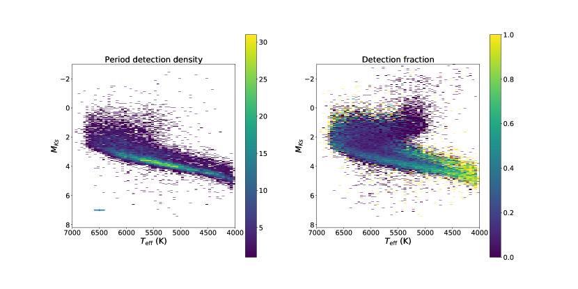
Figure 1: Left: $T_{\textrm{eff}}$-$M_{Ks}$ density plot of the sample of McQuillan et al. (2014) period detections. Color represents the number of objects in each bin. A binary sequence is clearly visible above the lower main sequence. Temperatures are from Pinsonneault et al. (2012). The bin size is 100 K in temperature and 0.02 mag in $Ks$-band absolute magnitude. A representative error bar is shown on the bottom left corner, although the vertical error bar is too small to be easily visible. Right: The variation in the McQuillan et al. (2014) period detection fraction across the $T_{\textrm{eff}}$-$M_{Ks}$ diagram.

The McQuillan et al. (2014) sample is shown in a $T_{\textrm{eff}}$-$M_{Ks}$ diagram in Fig. 1. One of the new results enabled by Gaia is that a binary sequence, located above the main sequence, is clearly seen. Also shown in Fig. 1 is the fraction of stars analyzed within each bin with period detections. The expected trends in activity are seen: period detections are common on the lower main sequence, and become relatively rare in evolved stars. The bulk of the period sample are solar analogs, reflecting the underlying Kepler sample.

2.5 Spectroscopic Parameters

We draw our spectroscopic sample from the Data Release 14 (Abolfathi et al., 2018) of the APOGEE survey (Majewski et al., 2017). The workhorse behind the survey is the APOGEE spectrograph, a high-resolution ($R\sim 22,000$) multi-fiber near-infrared spectrograph (Wilson et al., 2010) mounted on the SDSS 2.5-meter telescope at Apache Point Observatory (Gunn et al., 2006).

Reduction of the APOGEE data takes place in three main stages. First, individual visit spectra are reduced, including detector calibration, bad pixel masking, wavelength calibration, sky subtraction, and determination of individual radial velocities through cross-correlation of template spectra. Second, the individual spectra are combined by correcting for radial velocity differences between the exposures, either by cross-correlating with each other, or with template spectra, whichever leads to a smaller scatter (Holtzman et al., 2018). The full process is detailed in Nidever et al. (2015).

The final step is the extraction of stellar parameters and chemical abundances by the APOGEE Stellar Parameter and Chemical Abundances Pipeline (ASPCAP) (García Pérez et al., 2016). ASPCAP measures stellar parameters by performing a chi-squared minimization (Allende Prieto et al., 2006) over a 6-dimensional space of $T_{\textrm{eff}}$, $\log g$, [M/H], [$\alpha$/M], $v\sin i$, and microturbulent velocity. Once those six parameters have been determined, ASPCAP measures abundances for individual elements, including [Fe/H].

After determination of the stellar parameters and chemical abundances, the effective temperatures are calibrated to the photometric system of González Hernández & Bonifacio (2009) using a metallicity-dependent offset, and the abundances are calibrated to provide homogeneous results within clusters. After calibration, the scatter between the calibrated and photometric temperatures were found to be a function of $T_{\textrm{eff}}$, ranging from 130 K at 5500 K down to 85 K at 4000 K (Holtzman et al., 2018). The statistical uncertainty in [Fe/H] was measured to be 0.009 dex (Holtzman et al., 2018), but the systematic uncertainty is likely closer to 0.1 dex (Serenelli et al., 2017).

We inspected the fits to a set of spectra representative of targets flagged by the ASPCAP pipeline as having potential quality problems. A small fraction (2.5%) of targets have the STAR_BAD quality flag enabled. Visual inspection of a representative sample of spectra indicated that the flag was largely the result of poor subtraction or normalization of the spectrum in the pipeline, or due to poor model fits on the cool ($T_{\textrm{eff}}<4250\textrm{ K }$) end. We exclude these from our analysis. A substantially larger fraction of targets (14%) have the STAR_WARN quality flag enabled. Visual inspection of a representative sample of these spectra indicated that the fits reasonably resembled the underlying spectra. We include all targets with the STAR_WARN quality flag enabled.

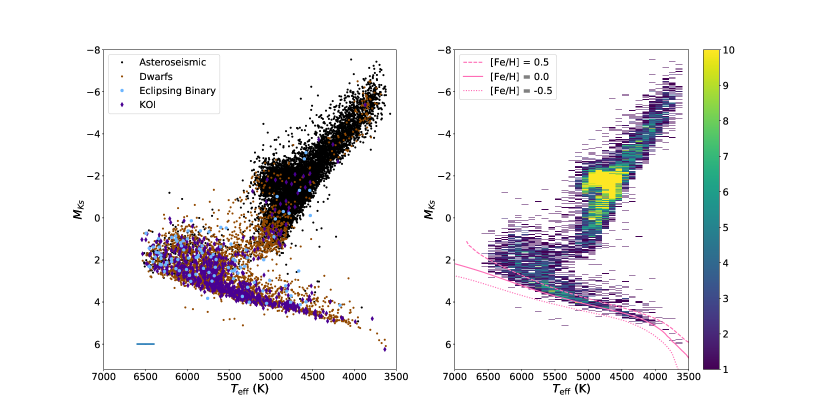
Figure 2: Left: $T_{\textrm{eff}}$-$M_{Ks}$ diagram for the APOGEE observations of Kepler targets. Asteroseismic targets are shown as black dots. The dwarf sample is shown as brown dots. The light blue circles indicate eclipsing binary targets and purple dots are Kepler Objects of Interest. A binary sequence is clearly visible on the lower main sequence. Temperatures are spectroscopic APOGEE temperatures. A representative error bar for the cool dwarf sample is shown in the bottom-left corner, although the vertical error bar is too small to be easily visible. Right: A density plot of the full APOGEE sample. To preserve the dynamic range of the dwarf sequence, the red clump was allowed to saturate. The bin size is 100 K in temperature and 0.02 mag in $Ks$-band absolute magnitude. 1 Gyr MIST isochrones with $[Fe/H]=0.5\textrm{ (dashed)},0.0\textrm{ (solid), and }-0.5\textrm{ (dotted)}$ are displayed in pink.

Fig. 2 shows all Kepler targets with observed spectroscopic temperatures in the APOGEE DR14, color-coded by observing program. One of the driving efforts for Kepler field observations has been the spectroscopic characterization of asteroseismic targets, shown as small black dots (Zasowski et al., 2017; Pinsonneault et al., 2018); 11,734 targets are part of that sample. The asteroseismic sample is substantially biased toward giants and subgiants due to their high amplitude oscillations. A complementary program proposed to observe the remaining portion of the Kepler sample cooler than 6500 K and brighter than $H<11$, make up an additional 3193 targets, shown as small red dots. An additional 695 targets were part of an effort to characterize Kepler planet hosts with $H<14$, shown as purple diamonds. The remaining 102 targets were targeted to follow-up eclipsing binaries (Prša et al., 2011; Slawson et al., 2011), and are shown as light blue circles.

The bulk ($\sim 80\%$) of the cool dwarfs ($T_{\textrm{eff}}<5250$ K were observed through the cool dwarf programs. These were large magnitude-limited surveys targeting objects with photometric $T_{\textrm{eff}}<6500$ K, photometric $\log g\leq 3.5$, and $H>11$ mag. This is expected to be our least biased sample because there are only course astrophysical constraints on the parameters. Much of the remaining sample ($\sim 17\%$) consists of follow-up observations to Kepler Objects of Interest. These observations go much deeper, down to $H=14$ mag. The inferred presence of a planet implies that this sample is likely to be biased toward high-metallicity and single stars. Lastly, the eclipsing binaries make up the rest of the sample, whose only criterion is that eclipses are found in the Kepler light curves. Because we do not want to bias our sample against binaries, include them even though they are few in number.

2.6 Eclipsing Binaries

When selecting the sample to perform their periodogram analysis, McQuillan et al. (2014) excluded known eclipsing binary targets to avoid confusing the eclipse signal as a rotation signal, which biases the rotation sample against close binaries. To correct for this bias, we include the Kepler Eclipsing Binary sample (Prša et al., 2011; Kirk et al., 2016), with the assumption that the short-period eclipsing binaries are synchronized.

With Kepler’s continuous monitoring and a long baseline of 4 years, the eclipsing binary sample for orbital periods on the order of 20 days should be complete (Kirk et al., 2016). Most eclipses were identified by the main Kepler pipeline (Jenkins et al., 2010). Orbital periods were measured using a neural network trained on synthetic eclipsing binary data (Prša et al., 2008). We downloaded the eclipsing binary catalog V3 from the Villanova web site, on June 3, 2016.

3 Data Analysis

The fundamental classification in this analysis is to distinguish photometric binaries from the rest of the sample. The crucial quantity to make this distinction is the vertical displacement above the single-star sequence. Vertical displacement is a standard measure of binarity in clusters (Mermilliod et al., 1992), where the single-star sequence can be described by a stellar population with a unique age and metallicity. Equal-mass binaries would lie 0.75 mag above the single-star sequence, while equal-mass triples would be 1.25 mag above. Measuring the vertical displacement for a field population is more challenging, because the field consists of heterogeneous ages and metallicities. There is a field turn-off, however, and for sufficiently cool dwarfs there is a well-defined unevolved main sequence that is an analog of the cluster case. We therefore search for the temperature domain where age effects are minimized, and where the natural width of the unevolved main sequence can be confidently measured to identify field binaries.

The vertical displacement is a difference of two quantities: the measured $Ks$-band luminosity of a star, and the inferred $Ks$-band luminosity of a single star with the same temperature and metallicity as the original one at a reference age. The former is a well-constrained and easily calculated quantity given the 2MASS photometry and the Gaia parallax; the latter requires a single-star model.

3.1 Stellar Model

We use the MIST (Dotter, 2016; Choi et al., 2016) isochrones to model the single-star lower main sequence. Bolometric corrections translating from evolutionary tracks to photometric bands are generated from ATLAS12/SYNTHE stellar atmosphere models (Kurucz, 1970, 1993). The solar abundance scale for the isochrones is from Asplund et al. (2009). For a full description of the MIST isochrones, we refer the reader to the source papers, as well as the MESA instrument papers (Paxton et al., 2011, 2013, 2015), which is the stellar model on which the isochrones are based. In order to characterize the vertical displacement, we select 1 Gyr isochrones as a baseline case. A sample 1 Gyr solar metallicity isochrone is shown in Fig. 2. As age effects in the domain of interest are by definition small, the precise choice of baseline age does not significantly impact our results (see Section 3.2).

3.2 Isolating Unevolved Stars

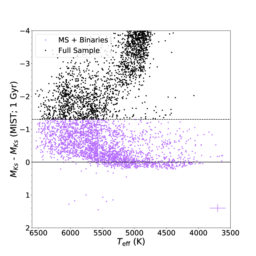
Figure 3: APOGEE temperature and vertical displacement above a 1 Gyr MIST isochrone matched to the APOGEE metallicity for the APOGEE-Kepler sample. In order to exclude evolved stars while preserving binaries and triples, we define the dwarf sample as targets less than 1.3 magnitudes more luminous than the metallicity-adjusted MIST isochrone (shown as violet points). A representative error bar for the full APOGEE dwarf sample assuming Gaussian uncertainties is shown in the lower right corner.

The effect of age is degenerate with that of binarity on the main sequence. Older stars at a given temperature are more luminous than younger stars. However, low mass stars experience little luminosity change over the lifetime of the Milky Way galaxy, therefore age will have a minimal impact on their apparent luminosity. As a result, the unevolved lower main sequence is an ideal regime for finding binaries. The transition where the age effect becomes small can be clearly measured by calculating the vertical displacement of the full APOGEE sample above a 1 Gyr isochrone, which is shown in Fig. 3.

For every star, the displacement is calculated by subtracting the luminosity of the 1 Gyr isochrone with the APOGEE-measured metallicity. F and G stars spread above the isochrone, which is expected because these stars evolve substantially over the age of the Milky Way. With the main sequence detrended, a visible binary sequence emerges at $\sim 0.75$ mag above the main sequence. Substantially above the main sequnce are the red giant branch stars, which we exclude by drawing a limit at 1.3 magnitudes above the main sequence. This limit cleanly excludes red giant branch stars while providing generous inclusion limits for binaries and potential triple systems.

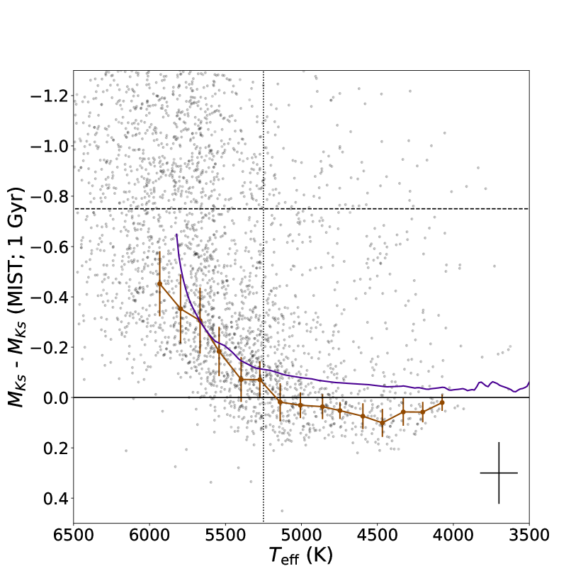
Figure 4: Age-imposed behavior for the dwarf sample with APOGEE temperatures. The purple line denotes the predicted luminosity excess of a 9 Gyr solar composition isochrone relative to a 1 Gyr baseline at fixed metallicity. The dashed line represents 0.75 mag, the limit for photometric binaries. The 25th percentile of the dwarfs in 15 temperature bins is shown in brown. The median absolute deviation of the least-luminous 50% of the bin is shown as the error bar. We draw a temperature threshold for the unevolved lower main sequence at 5250 K. A representative statistical error bar assuming Gaussian uncertainties is shown in the lower right corner.

To reduce the impact of age, we restrict ourselves to the unevolved lower main sequence, where age effects are small. We quantify the impact of age by predicting the vertical displacement of a 9 Gyr solar-composition MIST isochrone with respect to our 1 Gyr solar-composition MIST isochrone, shown in Fig. 4. The predicted displacement between the two isochrones is -0.20 mag at 5500 K, -0.11 mag at 5250 K, and -0.08 mag at 5000 K, showing a natural break at 5250 K.

We parametrize the behavior of the main sequence by splitting it into bins and calculating the 25th percentile of the luminosity excess in each bin. Each temperature bin contains a population of both binaries and single stars, with binaries having substantially higher vertical displacements. The 25th percentile statistic characterizes the main sequence in a way that is robust to the population of binaries, and has been used successfully in clusters (An et al., 2007). Even large departures from the assumed binary fraction should generally only affect the zero-point, but not the shape of the main sequence.

The detrended main sequence is generally flat at temperatures cooler than 5000 K with age effects becoming more important at hotter temperatures. The number of stars also increases substantially at temperatures above 5000 K. As a compromise between age effects and statistical power, we adopt a threshold $T_{\textrm{eff}}$ of 5250 K to denote the lower main sequence.

3.3 Metallicity Distribution

For the full McQuillan et al. (2014) sample, where individual metallicities are not available, we need to select an isochrone with a metallicity that is representative of the full sample. We do this by assuming that the metallicity distribution of the spectroscopic targets is representative of the full Kepler field.

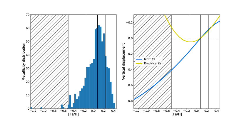
Figure 5: Left: Metallicity distribution of the Kepler cool dwarfs in the APOGEE sample, selected as having $T_{\textrm{eff}}<5250\textrm{ K }$ and a luminosity less than 1.3 mag above the single-star sequence. The thick black line denotes the median metallicity while the thin black lines denote the 1-$\sigma$ confidence intervals. The hatched region to the left of [Fe/H]=-0.5 denotes the metallicity beneath which the empirical correction in Fig. 6 is poorly constrained due to too few metal-poor stars. Right: The vertical displacement caused by assuming a single metallicity isochrone. The blue curve represents the difference between the derived $M_{Ks}$ assuming the median field metallicity and that for the true metallicity. The orange curve includes our empirical shape correction for metallicity, which removes most of the predicted width. The hatched region to the left of [Fe/H]=-0.5 denotes the metallicity beneath which the empirical correction is poorly constrained due to too few metal-poor stars.

Because we will mostly be concerned with the cool dwarfs, we check the metallicity distribution of dwarfs cooler than 5250 K, which is the temperature range of our sample. The metallicity distribution for that sample is shown in the left panel of Fig. 5. The median metallicity is 0.08, consistent with that observed for planet hosts by the California Kepler Survey (Petigura et al., 2017).

We check our assumption that the metallicity distribution for the full Kepler field is similar to the the spectroscopic catalog by comparing to results from the California Kepler Survey (CKS). The CKS observed a large (1305) sample of Kepler planet hosts, including a magnitude-limited sample with $Kp<14.2$ mag, which is substantially deeper than the APOGEE survey (Petigura et al., 2017). In order to test if the metallicity of a shallow survey, such as APOGEE, differs from the metallicity of a deeper survey, such as the CKS, we compare the metallicity distribution of the two surveys. As noted before, in Section 2.5, planet host surveys are likely to be biased toward higher metallicities. When applying the same temperature and evolutionary state cuts to the CKS, we find that the median metallicity is 0.05 dex. A 2-sample Anderson-Darling test finds that the two metallicity distributions are discrepant by 2-$\sigma$.

While the metallicity distributions of the two surveys are significantly different, the magnitude of the difference is small, even accounting for the fact that planet hosts should be more metal-rich than the overall sample. We therefore treat the shallow and deep samples as having the same metallicity. The small difference in mean metallicity will be corrected for by subtracting off a zero-point offset, which will be done in the following sections. As a result, we adopt the $\textrm{[Fe/H]}{}=0.08$ isochrone as the base isochrone for the photometric sample.

3.4 Correcting Metallicity Trends

Given a large, spectroscopically characterized sample with a well-populated main sequence, we can empirically determine how the main sequence behaves as a function of stellar parameters such as metallicity. Even modest differences between the theoretically predicted positions of isochrones and the data can impose structure on the detrended main sequence. Residual trends are not surprising because the NIR behavior of MIST isochrones have not been comprehensively tested at a wide range of metallicities (Choi et al., 2016). In order to achieve a truly detrended main sequence, we include both metallicity and temperature-dependent terms.

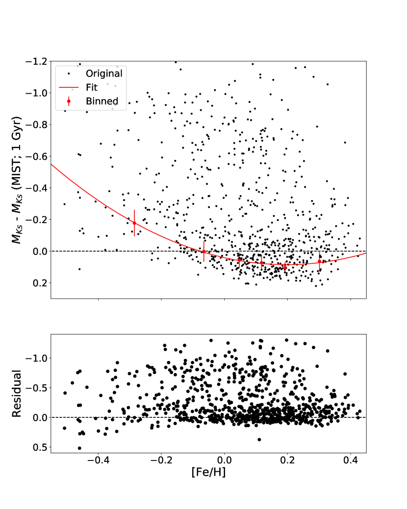
Figure 6: Top: Residual metallicity trend in the MIST metallicity-corrected vertical displacement. A quadratic trend remains over metallicity. The trend is characterized by fitting the sample to 5 bins with equal numbers of points. The 25th percentile of points denote the y-value of the bin while the mean temperature within each bins denotes the x-value. The best-fit relation is $\Delta M_{Ks}{}=-1.14\textrm{[Fe/H]}{}^{2}+0.448\textrm{[Fe/H]}{}+0.0411$. Red points mark the bins used for the fit. The median absolute deviation of the 50% of the sample showing the least luminosity excess within each bin is shown as an error bar. Three very low-metallicity points are not shown. Bottom: Residuals after correcting for the quadratic trend.

We find and correct for a residual quadratic trend in the vertical displacement of the main sequence over metallicity, shown in Fig. 6 for the spectroscopic sample. We fit the trend to 5 equally populated bins. We denote the metallicity of the bin as the mean metallicity of all stars in that bin, and the vertical displacement as the 25th percentile of all stars in that bin. For the purpose of selecting the optimal binning style, we quantified the goodness-of-fit using the median absolute deviation of the lowest 50% of the vertical displacements. The correction was mostly robust to the choice of binning; only the sparsely populated low-metallicity regime ($\textrm{[Fe/H]}{}<-0.5$) was sensitive to the details of binning. Because there are only eight objects in this metallicity range, our conclusions are not sensitive to their treatment.

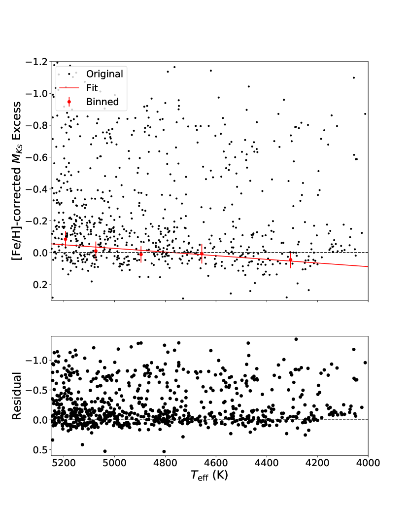
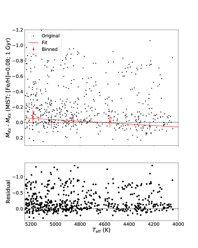
Figure 7: Top Left: Vertical displacement above a 1 Gyr, metallicity-adjusted MIST isochrone, empirically corrected for metallicity trends, for the cool sample with APOGEE temperatures. A slight linear trend in $T_{\textrm{eff}}$ was measured using five bins (shown in red). The best-fit relation is $\Delta M_{Ks}{}=-0.000114T_{\textrm{eff}}{}+0.546$ The median absolute deviation of the 50% of the sample showing the least luminosity excess within each bin is shown as an error bar. Bottom Left: The residuals after subtracting the linear trend. Not shown are the two most metal-poor objects in the sample, which have substantially large residuals. Top Right, Bottom Right: Same as left except using Pinsonneault et al. (2012) temperatures, and subtracting off a constant [Fe/H]=0.08 isochrone for all objects instead of a metallicity-adjusted isochrone. The best-fit relation is $\Delta M_{Ks}{}=-0.0000937T_{\textrm{eff}}{}+0.434$

Combining the two changes: subtracting only a single-metallicity isochrone and using the photometric temperatures yields the points in the right panel of Fig. 7. This sample still has a trend with temperature, that we remove using a linear fit, similar to that done for the spectroscopic sample.

3.5 Temperature Corrections

3.5.1 Spectroscopic Sample

After correcting the trend in metallicity, we correct a residual trend in $T_{\textrm{eff}}$, shown in Fig. 7 using a similar procedure. We take five equally-populated bins, and define the bin temperature and displacement using the mean within the bin and 25th percentile displacement within the bin. This trend is slight and can be subtracted using a linear fit. After performing these two corrections, we consider the main sequence to be flattened to its measured natural width, as seen in the bottom panel of Fig. 7. The persistence of the binary sequence in the residuals indicates that our corrections are meaningful.

3.5.2 Photometric Sample

The photometric sample in McQuillan et al. (2014) differs from the spectroscopic sample in two main ways: the lack of metallicity diagnostics, and the necessity of using photometric instead of spectroscopic $T_{\textrm{eff}}$. Both of these differences will increase the uncertainty of the inferred single-star $Ks$-band luminosity, and we measure their impact in the following analysis.

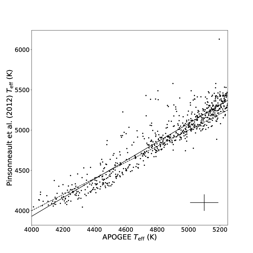
Figure 8: Comparison between the APOGEE spectroscopic $T_{\textrm{eff}}$ and the Pinsonneault et al. (2012) $T_{\textrm{eff}}$ for objects with $4000\textrm{ K }\leq\textrm{ APOGEE $T_{\textrm{eff}}${} }\leq 5250\textrm{ K }$. A linear fit for the temperature is shown as the solid line. The best-fit model is $T_{\textrm{eff,phot}}=1.153T_{\textrm{eff,spec}}-682.6$. The one-to-one line is shown as a dashed line. The scatter between the two datasets is 135 K. A representative error for both datasets is shown in the bottom-right corner.

We estimate the impact of the photometric temperatures by directly comparing the spectroscopic and photometric temperatures for the set of overlapping points shown in Fig. 8. Overall, the two temperature scales are reasonably correlated. There is a temperature scatter of 135 K between the two scales. Taking into account the 100 K uncertainty in the APOGEE $T_{\textrm{eff}}$ scale, by assuming the two uncertainties add in quadrature, this implies a 90K uncertainty in the Pinsonneault et al. (2012) temperatures, which agrees with the uncertainties expected from the photometric method.

3.6 The Impact of Metallicity on the Main Sequence Width

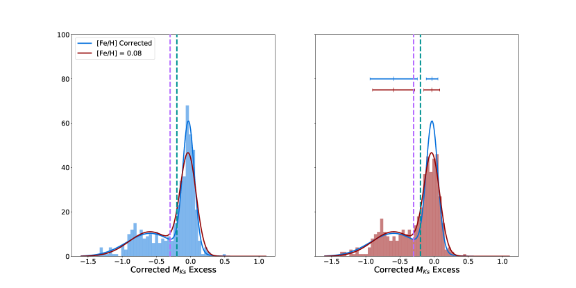
Figure 9: Left: Histogram showing the distribution of vertical displacements with isochrones corresponding to APOGEE metallicities. The blue curve denotes the best-fit double-Gaussian model to the distribution of vertical displacements. The red curve is a fit to the best-fit double-Gaussian model assuming a single metallicity (see right panel). Conservative and inclusive photometric binary thresholds at $\Delta M_{Ks}{}<-0.3$ mag and $\Delta M_{Ks}{}<-0.2$ mag are shown as violet and green dashed lines, respectively. The best-fit dispersion of the single-star Gaussian is 0.086 mag. Right: Histogram showing the distribution of vertical displacements with a $\textrm{[Fe/H]}{}=0.08$ dex isochrone. The red curve denotes the best-fit double-Gaussian model to the distribution of vertical displacements. The blue curve is a fit to the best-fit double-Gaussian model for isochrones adjusted for the APOGEE metallicity (see left panel). Conservative and inclusive photometric binary thresholds are shown as violet and green dashed lines, respectively. The best-fit dispersion of the single-star Gaussian is 0.117 mag. The blue points at the top of the plot show the mean and standard deviation of the single and binary Gaussian fits for the sample with metallicity information. The red points show the mean and standard deviation of the single and binary Gaussian fits for the sample without metallicity information.

Now that we have corrected vertical displacements over the 4000–5250 K temperature range, we can now compare the main-sequence width for the two datasets. Histograms for the spectroscopic and photometric samples over vertical displacement are shown in Fig. 9. We try to characterize the width of the two samples by fitting a double Gaussian to each histogram, and taking the width of the Gaussian centered on the main sequence as the uncertainty in the vertical displacement. Our fits indicate that the main-sequence width for the spectroscopic sample is 0.086 mag while the width for the photometric sample is 0.117 mag.

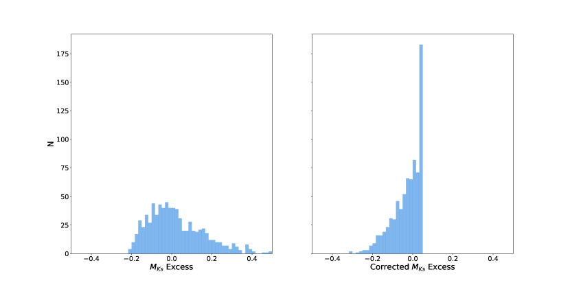
Figure 10: Left: The distribution of vertical displacements imposed by the metallicity distribution of the APOGEE sample using the raw MIST isochrones. All stars are assumed to have a known temperature of 5000 K. Not shown are two very metal-poor stars which are off the plot to the right. Right: Same as the left, except the MIST $Ks$-band magnitudes are corrected by the empirical correction in Fig. 6 and the two most metal-poor stars are off the figure to the left.

This modest increase in the width for the photometric sample is surprising, especially given the strong dependence of $Ks$-band magnitude on metallicity predicted by the MIST isochrones shown in the right panel of Fig. 5. We believe that the reduced width is real, and that the MIST bolometric corrections overestimate the dependence of $Ks$-band luminosity on metallicity. We demonstrate the metallicity dependence of the isochrones by measuring the main-sequence width for an artificial population of stars which differ only by metallicity. We assume all stars have a temperature of 5000 K, an age of 1 Gyr, and have metallicities drawn from the APOGEE cool dwarf metallicity distribution (shown in the left panel of Fig. 5).

We display two realizations of this population in Fig. 10: one using $Ks$-band magnitudes predicted by MIST (left), and another applying the metallicity-dependent correction in Fig. 6 (right). The main-sequence width of the two populations are 0.14 mag and 0.10 mag, respectively, indicating that the corrected distribution has a smaller width. As is evident from the corrected sample on the right side of Fig. 10, the reduction in the width of the main sequence is driven by a cutoff at large, positive vertical displacements. The origin of this cutoff comes from the metallicity-dependence of the empirical correction in Fig. 5; metal-poor stars are forced to smaller vertical displacements compared to the MIST predictions. We note that the MIST models predict that the metallicity dependence $Ks$-band is similar to the $V$-band, which indicates that the predicted width is a feature of the luminosity dependence of the main sequence locus, not a peculiar feature of the $Ks$-band bolometric corrections.

3.7 Characterizing the EB Distribution

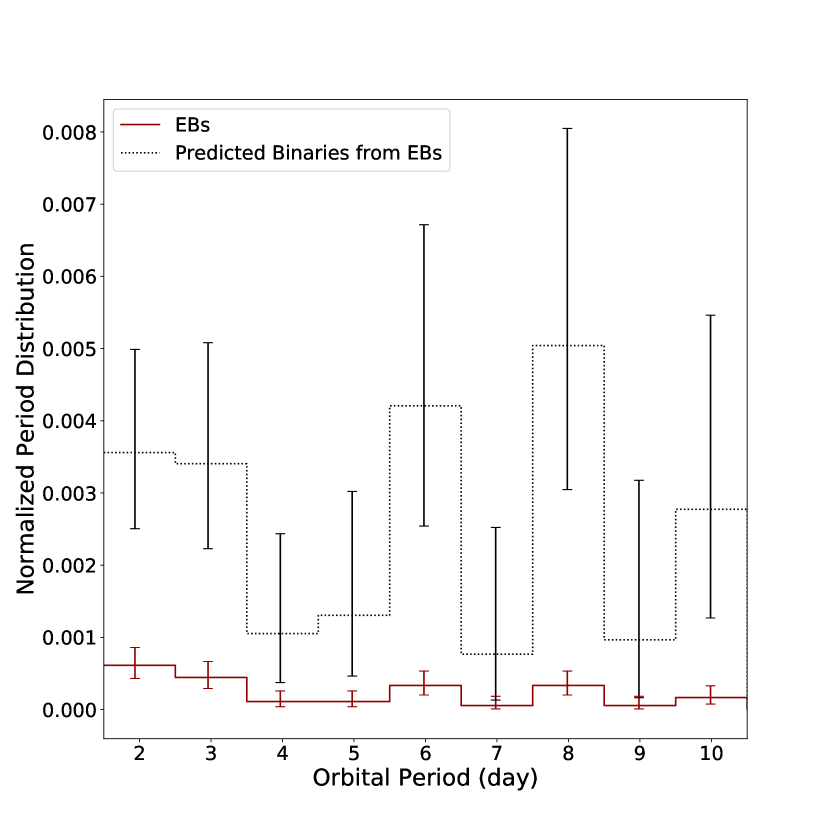
Figure 11: The observed period distribution of all eclipsing binaries with Pinsonneault et al. (2012) $T_{\textrm{eff}}$ < 5250 K and vertical displacement less than 1.3 mag is shown in red. The period distribution of the full binary distribution inferred from the eclipsing binaries is shown in black. The normalization factor is the total number of Kepler cool dwarfs. Error bars represent 1-$\sigma$ Poisson confidence intervals.

Kepler’s short 30 minute cadence allows it to detect essentially all eclipsing main-sequence binaries with periods less than 10 days (Kirk et al., 2016). Even the shortest-period systems become detectable through ellipsoidal variations rather than through eclipses. As a result of Kepler’s completeness at these short periods, the distribution of eclipsing binaries is solely determined by geometry, with an eclipse probability for circular orbits given as $(R_{1}+R_{2})/a$, where $R_{1}$ and $R_{2}$ are the primary and secondary radii, and $a$ is the semimajor axis of the orbit. This simple expression means that using the period distribution of the eclipsing binaries, as well as estimates for the masses and radii of the component stars, one can predict the expected period distribution of the full binary sample using just the eclipse probability. We use the expression assuming circular orbits, which is justified because short-period, low-mass systems are overwhelmingly observed to be circularized (Raghavan et al., 2010; Van Eylen et al., 2016).

We infer the primary radius by mapping temperature to radius using the MIST isochrones. Depending on whether the analysis is done in the context of the spectroscopic sample or the photometric sample, the appropriate temperature is used.

To simplify the calculation, we assume that the secondaries are half as massive as the primaries, which is generally consistent with a flat mass-ratio distribution (Raghavan et al., 2010). More massive secondaries would reduce the predicted number of non-eclipsing systems.

While the semimajor axis isn’t directly observable, we infer it from the orbital period using Kepler’s third law, which requires masses for the two components. We infer masses using a method similar to the radii above: the primary mass is mapped from $T_{\textrm{eff}}$, while the secondary mass is assumed to be half of the primary’s mass.

Given these assumptions, an estimate of the orbital period distribution for all short-period Kepler binaries on the unevolved lower main sequence is shown in Fig. 11. The eclipsing binaries range from making up almost 15% of the total population of binaries in the shortest-period bin in Fig. 11 to 6% in the longest-period bin, hence they are not a negligible segment of the population. McQuillan et al. (2014) excluded eclipsing binaries from their analysis of rotation in the Kepler field due to concerns that the eclipse signal would dominate the period. In order to obtain an unbiased view of the binary population at short periods, we calculate vertical displacements for the Kepler eclipsing binaries as well and include them in our statistical analysis in Section 4. This treatment assumes that orbital period is identical to the rotation period, which should certainly be true for synchronized systems; we address the question of synchronicity directly in Section 4.2. By combining the bins in Fig. 11, the eclipsing binary population predicts that $2.1\%\pm 0.4\%$ of the cool Kepler targets should be binaries with periods between 1.5–10 days.

3.8 Binarity and Temperature Estimation

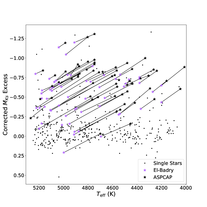
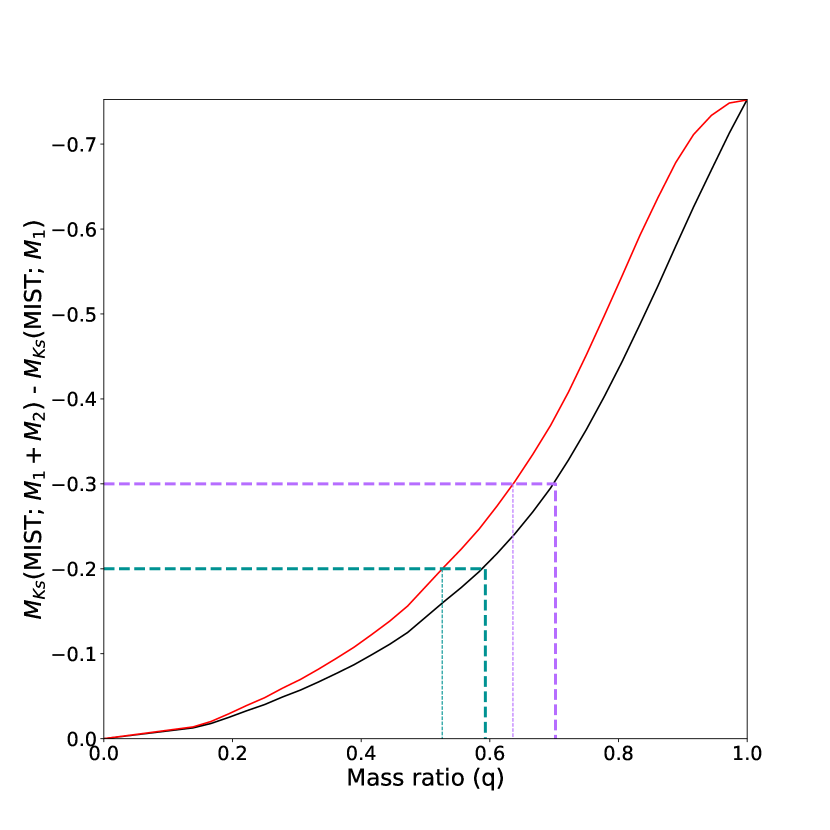
Figure 12: Left: The sample of APOGEE targets analyzed by El-Badry et al. (2018b) for spectroscopic signs of a companion. Black points indicate the APOGEE DR14 values for the targets. Violet points indicate the revised temperatures, and the $Ks$-band luminosity excess derived from the revised temperature and metallicity in El-Badry et al. (2018b). Right: Vertical displacement of a binary with a 0.7 M_☉, solar metallicity primary as a function of mass ratio using MIST models (black line). The violet and green dashed lines denote the mass-ratio at which the vertical displacement exceeds -0.3 and -0.2 mag, which are mass-ratios of 0.69 and 0.58. The red line denotes the same vertical displacement, but taking into account distortions in the photometric $T_{\textrm{eff}}$ caused by binarity. The mass-ratios corresponding to the conservative and inclusive thresholds are 0.64 and 0.53.

While we generally assume that objects showing large vertical displacement are binaries, our sample includes an abundance of systems with vertical displacements greater than 0.75 mag, some greater than even 1.3 mag. One obvious explanation for these systems is that they are multiple systems where each component contributes substantially to the luminosity. One other explanation is that the secondary biases the observed temperature to be cooler than the actual primary temperature causing the single-star luminosity to be underestimated. This phenomenon is expected to occur for both photometric and spectroscopic temperatures (Pinsonneault et al., 2012; El-Badry et al., 2018a).

We test the effect of binarity on the estimated spectroscopic temperature by using APOGEE DR13 targets whose spectra were fit for multiple components (El-Badry et al., 2018b). In cases where a two-component fit was favored, temperatures were published for both the primary and secondary. With Gaia DR2 parallaxes, we can test how often two photometric components were successfully detected. All the DR13 objects analyzed by El-Badry et al. (2018b) which overlap with the cool dwarf rotation sample are shown in Fig. 12 with both the ASPCAP and decomposed primary temperatures.

The overall behavior in the El-Badry et al. (2018b) sample shows that the effect of binarity on spectroscopic temperatures is substantial. For many of the intermediate mass-ratio objects, there is a temperature discrepancy of several hundred Kelvin, leading an overestimation of the $Ks$-band vertical displacement by up to 0.3 mag. The difference in temperature is less severe for targets with high luminosity excesses, which is to be expected because the two stellar components would have similar spectra. However, the effect is still not negligible. For the purpose of flagging photometric binaries, this effect is beneficial, as it increases the contrast of lower mass-ratio systems against the single stars. To characterize the luminosity-ratio of the components, however, the offset of temperatures would need to be taken into account.

While the two-component fit produces results that overall seem reasonable, many of its decompositions were not compatible with the vertical displacement. Many of the photometric binaries were not flagged as requiring two-component fits. Additionally, two of the targets showing essentially no vertical displacement were flagged as having substantial modifications to the temperature from a companion. Nonetheless, we consider the results of the analysis by El-Badry et al. (2018b) to impressive given that they did not make use of Gaia parallaxes. Future analyses may want to make use of the vertical displacement when flagging spectra for multiple-component fits.

We also investigate the impact of binarity on the vertical displacement using photometric temperatures. Unlike El-Badry et al. (2018b), who directly fit two-component models to the full spectra, we instead are interested in how companions generically affect the vertical displacement through temperature. We explore by building a toy model of a binary using MIST isochrones, and perturbing the observed temperature using a color-$T_{\textrm{eff}}$ relation. Because the Pinsonneault et al. (2012) temperatures were derived using griz colors, we opt to use the $(g-i)$-$T_{\textrm{eff}}$ relationship to probe the impact of binarity on the temperature. Redder colors are more sensitive to low-mass binary companions, so we choose the $(g-i)$ color as the reddest color that maintains high photometric precision. The effect of binaries should be less pronounced for bluer color-temperature relations.

To isolate the effect of temperature offsets on vertical displacement, we adopt a standard primary with a mass of 0.75 $M_{\sun}$ and solar metallicity, and use the MIST isochrones to calculate an intrinsic $g-i$ color. We derive a temperature for the star by fitting a 5th-degree polynomial between $\tfrac{5040K}{T_{\textrm{eff}}}$ and $(g-i)$ using the MIST synthetic photometry. We then generate secondaries with a range of mass-ratios, and add their flux to the primary flux, and infer a composite temperature based on the combined flux. Lastly, the composite temperature is then used to calculate the reference K-band magnitude as opposed to the true primary temperature. The relationship between vertical displacement and mass-ratio without taking into account the color of the secondary is shown in black in Fig. 12. The relationship behaves as expected, with a sharp increase at high mass-ratio until 0.75 mag. When the color of the secondary is taken into account, we get the red curve in the left panel of Fig. 12. The impact of the binary on photometric temperatures is substantially smaller than for the spectroscopic temperatures, only increasing the vertical displacement by up to 0.1 mag. Our toy model also predicts that the temperature deviations are so small compared to the slope of the main sequence that the vertical displacement never exceeds 0.75 mag, as is observed in the spectroscopic case.

Because the effect of binarity on photometric temperature only imparts small deviations for the vertical displacement, we claim that the objects which lie substantially above the photometric binary sequence are true multiple systems, or systems with an unusual evolutionary history, such as mass-transfer from a companion.

4 Results and Discussion

4.1 Vertical Displacements of Rapid Rotators

After successfully calculating the vertical displacement of the full sample, we now attempt to distinguish between single and binary stars. As noted in Section 3.6, the 1-$\sigma$ width of the single-star sequence were 0.086 mag with known metallicity, and 0.117 mag when metallicity was unknown. To implement a uniform photometric binary cut for both the spectroscopic and photometric samples, we will assume a measured width of the main sequence of 0.1 mag. To prevent age effects from biasing the results, we only performed statistics in the 4000–5250 K range.

The primary quantity we use to characterize the binarity of our samples is the photometric binary fraction, defined as the fraction of targets within a given period range that have a vertical displacement above a certain threshold. To show that our findings are robust to the choice of photometric binary threshold, we report photometric binary fractions for two photometric binary thresholds: an inclusive 2-$\sigma$ threshold and a conservative 3-$\sigma$ threshold, which turn out to be displacement cuts of 0.2 and 0.3 mag.

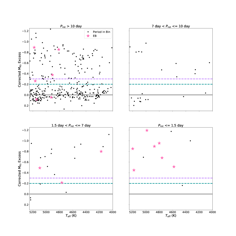
Figure 13: Top Left to Bottom Right: Vertical displacement of cool APOGEE targets with McQuillan et al. (2014) periods >10 days, between 7–10 days, 1.5–7 days, and <1.5 days. Pink stars denote eclipsing binaries with orbital periods within the same ranges. The green and purple lines denote the inclusive and conservative photometric binary thresholds, respectively. The temperatures are from APOGEE.

For both binarity thresholds, the well-characterized APOGEE sample illustrates the differences in binarity between slow and rapid rotators, as shown in Fig. 13. For the purpose of illustration, we divide the sample into four period ranges, with boundaries of 1.5, 7, and 10 days. We draw a short-period limit for our analysis at 1.5 days because we want to eliminate potential contamination from ellipsoidal variables and semidetached systems (Van Eylen et al., 2016). We find 7 days to mark the transition from a binary-dominated synchronized population to a single-star dominated population (see below). And 10 days is the theoretically and observationally-motivated boundary in orbital period where synchronization should take place (Claret & Cunha, 1997; Lurie et al., 2017).

Even by eye, it is striking in Fig. 13 that nearly all of the rapid rotators with periods between 1.5–7 days are photometric binaries, in contrast to the slow rotators with periods greater than 10 days, which have a distinct single star sequence. The depletion of the single-star sequence in the short-period regime is likely due to angular momentum loss due to stellar winds acting over a billion years. The transitional periods between 7–10 days have a binary fraction intermediate to the rapid and slow regimes. The bin with periods shorter than 1.5 day is not expected to behave like detached, eclipsing binaries due to potential contamination from contact binaries, ellipsoidal variables and blended pulsators (Van Eylen et al., 2016).

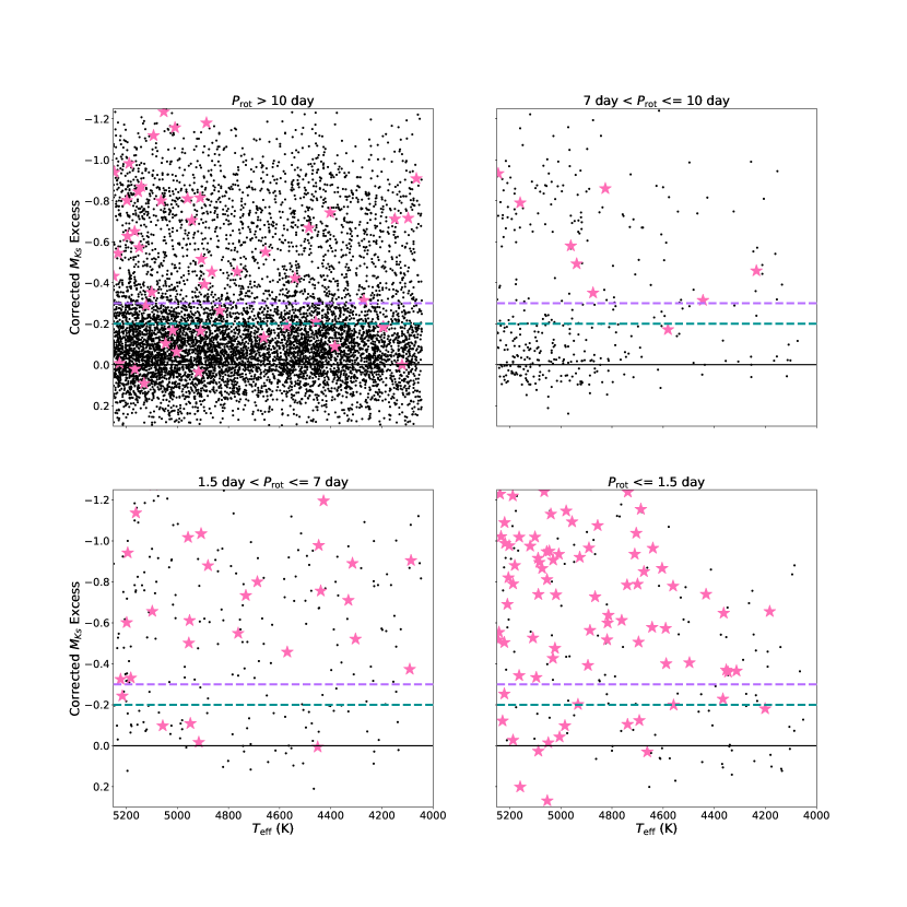
Figure 14: Top Left to Bottom Right: Vertical displacement of all cool McQuillan et al. (2014) targets in period ranges >10 days, 7-10 days, 1.5-7 days, and <1.5 days. Pink stars denote eclipsing binaries with orbital periods within the same ranges. The green and purple lines denote the inclusive and conservative photometric binary thresholds, respectively. The temperatures are from Pinsonneault et al. (2012).

While the spectroscopic sample shows broad trends between rotation and binarity in wide period ranges, the substantially larger photometric sample is needed to effectively characterize the rapid rotators. The vertical displacement of the photometric sample in the same period ranges as before is shown in Fig. 14. With a substantially larger number of objects, the absence of the single-star sequence in the panel of rapid rotators is starker.

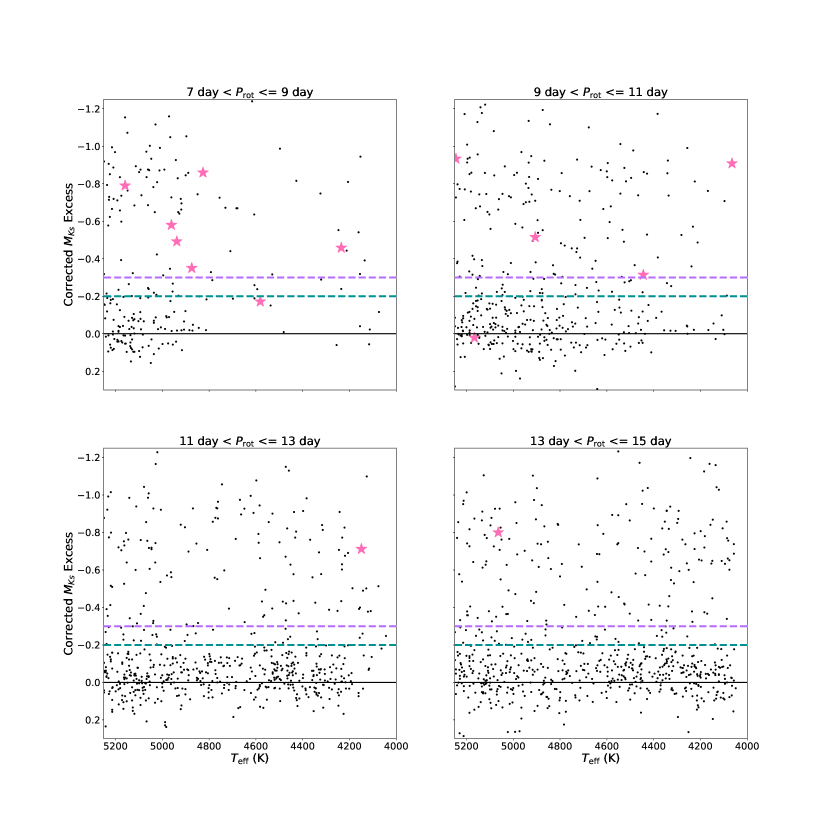
Figure 15: Same as Fig. 14 except with the period ranges 7–9 days, 9–11 days, 11–13 days, and 13–15 days.

The behavior of the single-star sequence is shown in Fig. 15, where we show a narrower range of periods in the transition region. The single-star sequence appears in the hottest stars first in the panel with the most rapidly rotating systems. Cooler stars appear on the single-star sequence as longer periods. The trend that hotter stars in the field rotate more quickly than the cooler stars is consistent with the overall trend in temperature seen in McQuillan et al. (2014).

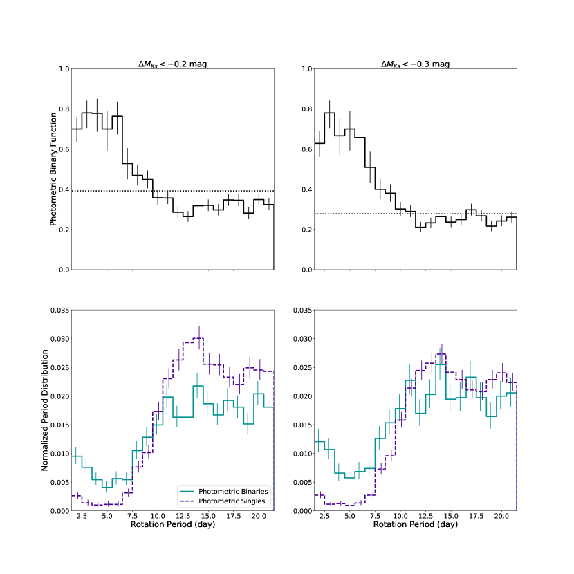
Figure 16: Top Left: The photometric binary function for the inclusive photometric binary threshold ($\Delta M_{Ks}{}<-0.2$ mag). The photometric binary fraction for the full sample analyzed by McQuillan et al. (2014) is shown as the dotted line. Error bars are 1-$\sigma$ binomial confidence intervals. Top Right: Same as the previous plot, except using the more conservative threshold ($\Delta M_{Ks}{}<-0.3$ mag). Bottom left: The period distribution of the photometric binary (solid green) and photometric single (dashed purple) samples, each normalized by the total number of photometric binaries and photometric single stars analyzed by McQuillan et al. (2014), respectively, using the inclusive photometric binary threshold. Error bars are 1-$\sigma$ Poisson confidence intervals. Bottom Right: Same as the previous plot, except with the more conservative vertical displacement threshold.

In order to understand the low-period edge of the single-star population, as well as the cutoff period for the tidally-synchronized binaries, we need to quantify the behavior illustrated in Figs. 14 and 15. While we proceed using only the photometric sample to derive statistics, we note that repeating the analysis with the much smaller spectroscopic sample yields consistent, but less constrained results.

One measure to trace changes in behavior between the binaries and single stars with rotation is what we call the “photometric binary function”, which denotes the photometric binary fraction as a function of rotation period. The photometric binary function is shown in the top row of Fig. 16. As was qualitatively shown in Fig. 15, the photometric binary function is high for rotation periods below 7 days, above which it begins to decrease, which is expected for the contribution of the single-star tail. However, the photometric binary function does not reach the mean binarity of the full sample until around 9–11 days, after which the single-stars dominate the population.

To quantify the significance of the excess binary fraction in the rapid rotators, we compare the photometric binary fraction of the short-period bin to the binary fraction of the full sample. As mentioned previously, we include the Kepler eclipsing binaries, to accurately characterize the binarity of short-period systems.

We also find that the period dependence of the photometric binaries and photometric singles differ in the short-period domain. The period distribution of photometric binaries as well as the period distribution of photometric single stars is given in the bottom row of Fig. 16 as a function of period for both the inclusive and conservative photometric binary thresholds. The number of photometric binaries and photometric single stars both decrease in the short-period regime compared to the long-period regime; however the photometric single stars decrease much more steeply than the photometric binary stars. The sudden drop in photometric single stars implies a mixed photometric binary/single population at long periods, and a binary-dominated population at short periods. As seen with the photometric binaries, a tail of single stars appears at rotation periods greater than 7 days for both the inclusive and conservative photometric binary thresholds. The relative contributions of photometric and single stars then become fixed past 11 days, consistent with the flattening of the photometric binary fraction.

4.2 Comparison with Eclipsing Binaries

Given the radical difference in behavior between the photometric binaries and photometric single stars between the short- and long-period regimes, we propose that the rapid rotators are dominated by tidally-synchronized binaries. The short-period systems that do not show significant vertical displacement are likely low mass-ratio systems. This interpretation of the photometric singles in the rapid rotators is supported by comparing the photometric binary fraction of the eclipsing binaries to that of the rapid rotators. The photometric binary fraction of the eclipsing binaries with orbital periods between 1.5–7 days is $83^{+7}_{-10}\%$ with the inclusive threshold and $76^{+8}_{-11}\%$ with the conservative threshold, while the photometric binary fraction of the rapid rotators with rotation periods between 1.5–7 days is $67^{+3.3}_{-3.5}\%$ with the inclusive threshold and $59^{+3.6}_{-3.6}\%$ with the conservative threshold. Given the uncertainties, the two photometric binary fractions are just outside of one sigma away from each other. A slightly higher photometric binary fraction for the eclipsing binaries is also to be expected because photometric binaries have larger secondaries, hence have a larger eclipse probability.

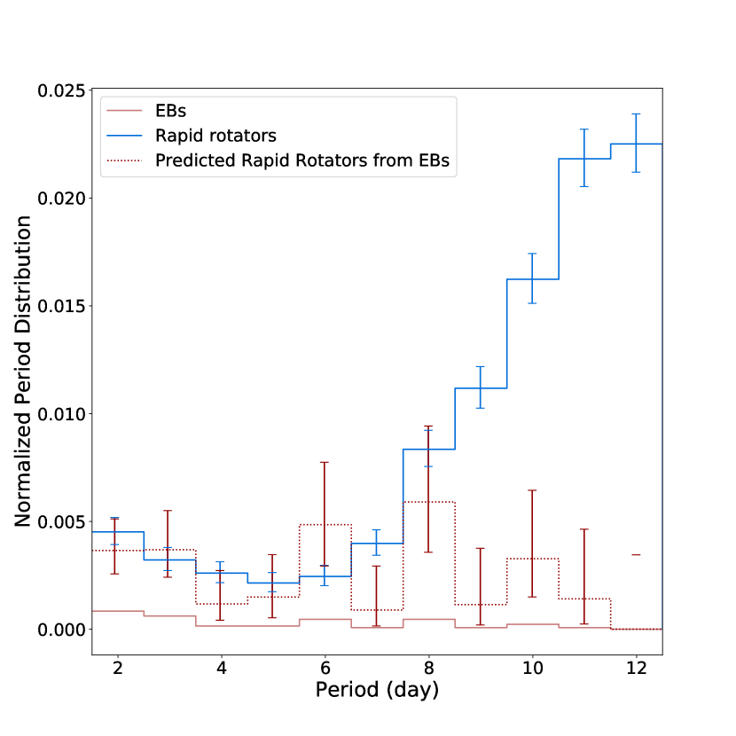
Figure 17: Comparison of the rapid rotator and eclipsing binary period distributions. The period distribution of the McQuillan et al. (2014) sample is shown as a blue solid histogram, while the period distribution of the eclipsing binaries is shown as the red histogram. Both distributions are normalized to the total number of objects analyzed by McQuillan et al. (2014) and in the EB catalog. The predicted EB distribution (red dashed line) uses the observed EB orbital period distribution to predict the period distribution of binaries inclined enough to show starspot modulation, but not inclined enough to eclipse. Error bars represent 1-$\sigma$ Poisson confidence intervals.

The rotation period distribution of rapid rotators also agrees well with the expected orbital period distribution of a population of non-eclipsing binaries, providing further evidence that the rotation period and orbital periods are identical. We demonstrate this finding by comparing the observed rotation sample to a predicted population of non-eclipsing binaries derived using the eclipsing binary sample and the geometrical corrections in Section 3.7. In addition to the corrections from eclipse probabilities, we correct for the detectability of rotation periods caused by inclination. K2 observations of the Pleiades found that 8% of the sample did not show variations due to starspots (Rebull et al., 2017), which is similar to the fraction of objects previously found to have inclinations too high to show starspots (Jackson & Jeffries, 2010). Since rotation periods in the Pleiades are on the order of several days, comparable to the rotation periods in this sample, we treat 8% of the total sample as being too highly-inclined to have observable starspot periods. Given these assumptions, and the observed population of eclipsing binaries, the predicted orbital period distribution of non-eclipsing binaries in Fig. 17.

The orbital and rotation period distributions match well up to 7 days, indicating that the rotational period distribution reflects the orbital period distribution for the eclipsing binaries. The period at which the data diverges from the prediction is also similar to the period where the binary fraction drops in Fig. 16. The concordance of these two periods suggests that the short-period systems follow a rotational period distribution compatible with the orbital period distribution of eclipsing binaries, while the long-period systems follow a different rotational period distribution. Our physical interpretation for this phenomenon is that the short-period systems are tidally-synchronized binaries, which remain synchronized at least through an orbital period of 7 days. At periods longer than 7 days, the picture becomes more complicated, with the transition from synchronized to unsynchronized systems overlapping with the tail of rapidly-rotating single stars and wide binaries. Determining the synchronization cutoff period will require disentangling these populations.

Assuming that the rapid rotators and eclipsing binaries are two disjoint samples of the same population between 1.5–7 periods, we can combine both samples to generalize properties of the rotation sample studied by McQuillan et al. (2014), assuming that they would have correctly identified the rotation period of the eclipsing binary as the orbital period. We calculate that $1.9\pm 0.1\%$ of the sample analyzed by (McQuillan et al., 2014) have rotation periods between 1.5–7 days. As noted previously, the rapid rotators and eclipsing binaries should be sensitive to 92% of the most inclined systems. Correcting for the low-inclination systems yields that $2.0\pm 0.1\%$ of systems analyzed by McQuillan et al. (2014) should be synchronized binaries with orbital periods between 1.5–7 days. Therefore, synchronized binaries are expected to be present in rotation samples at that level. Future binary surveys may use photometric binaries to select systems appropriate for further study. In a sample of pure photometric binaries, the short-period systems will be more prominent; systems with rotation periods between 1.5–7 days make up $3.4\pm 0.3\%$ of photometric binaries under our inclusive threshold, and $4.5\pm 0.4\%$ under our conservative threshold.

4.3 The High Photometric Binary Fraction

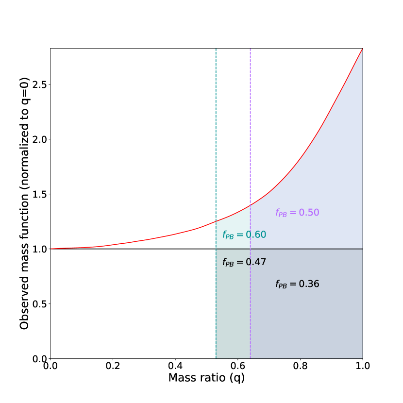
Figure 18: Observed mass distribution for a magnitude-limited binary population with a flat mass function and constant spatial density. Without considering the Malmquist bias, the flat mass distribution is given as the horizontal black line. The fraction of photometric binaries for the flat mass function is 36% for the conservative threshold and 47% for the inclusive threshold. The red line denotes the observed mass distribution taking into account that higher mass-ratio binaries are seen out to larger distances. Taking into account the Malmquist bias raises the photometric binary fraction to 50% for the conservative threshold and 60% for the inclusive threshold.

With evidence that the short-period systems are dominated by binaries, we can compare the observed photometric binary fraction to that expected from a flat mass-ratio distribution. As noted in the previous section, the observed photometric binary fraction for the rapid rotator sample is 59% using the conservative threshold and 67% using the inclusive threshold. If we assume a flat mass-ratio distribution, as shown in Fig. 18, we expect the photometric binary fraction to equal the fraction of systems with mass-ratio large enough to exceed the given vertical displacement threshold, denoted as the dark shaded region. Based on the model presented in Fig. 12, the mass-ratio limits for our thresholds according to MIST models are 0.64 for the conservative threshold and 0.53 for the inclusive threshold. These result in expected photometric binary fractions of 36% and 47% for the conservative and inclusive thresholds, respectively. Both are substantially smaller than the observed fractions.

One factor which could raise the observed binary fraction is Malmquist bias. While the Kepler selection function is heterogeneous and complex, distances were not available for the bulk of the sample at the time. As a result, photometric binaries, which are intrinsically more luminous than single stars, would be detected out to a larger volume.

We illustrate the effect of Malmquist bias for an artificial population with constant spatial density and a flat mass function in the right panel of Fig. 18. As expected, the observed mass function increases because the photometric binaries are detected in larger volumes. Using the same minimum mass-ratio as with the flat mass-ratio distribution, including the Malmquist bias increases the photometric binary fraction from 37% to 50%, which is much closer, but still smaller than the observed photometric binary fraction by 2-$\sigma$. We note that this treatment of Malmquist bias is an upper limit to the effect because the true spatial density of the Kepler field should encounter an expoential dropoff, which would reduce the number of distant photometric binaries.

The tension between the predicted and observed photometric binary fractions still exists even when the most common selection effects are taken into account. It’s likely that resolving this will requires either that the mass-ratio for synchronized binaries is tilted toward higher-mass systems, that there are more subtle selection effects in the Kepler sample, or that there are higher-order systems which aren’t accounted for in our simple toy models. Attempting a detailed reconstruction of the intrinsic mass-ratio distribution of tidally-synchronized binaries is beyond the scope of this analysis.

4.4 The Synchronization Threshold

The 7 day limit that we get for the synchronization period cutoff is compatible with previous theoretical expectations. The original formulation by Zahn (1977) included an expression for the synchronization timescale for a binary system given as $t_{sync}=10^{4}((1+q)/2q)^{2}P^{4}/R^{6}$ where $t_{sync}$ is in years, $q$ is the mass-ratio, $P$ is in days, and $R$ is the radius in solar radii. For a 4 Gyr old equal-mass field binary, this corresponds to a synchronization period of 15 days, which is well within the constraints. Claret & Cunha (1997) revisited the formulation of Zahn (1977) and instead advocated substituting a different expression for the apsidal motion constant which made tidal dissipation on the main sequence a factor of 5 smaller. The new expression corresponds to a synchronization period of 10 days, which is also consistent with our findings.

From this calculation, it’s clear that the 7-day limit we observe is caused by the age distribution of the Kepler field as opposed to the tidal properties of the binaries. In order to probe the synchronization threshold for close binaries, rotation periods will be needed for a substantially older population than the Kepler field. This may be achieved through a Kepler-like survey for a specifically older stellar population, or by filtering out young stars through kinematics.

5 Conclusion

We calculated $Ks$-band luminosity excesses above the main sequence for the full McQuillan et al. (2014) sample. As seen in both a spectroscopically-characterized subset as well as in the general sample, rapid rotators with periods between 1.5–7 days show substantially larger luminosity excesses than the slower rotators. At periods longer than 7 days, the rapidly rotating tail of the single-star population grows more numerous before dominating the sample at periods longer than 9 days.

We propose that the excess of binaries among rapid rotators is a sign that tidally-synchronized binaries dominate the short-period end of the rotation distribution. When comparing the rotational period distribution of the rapid rotators to the orbital period distribution of Kepler eclipsing binaries, we find that the rapid rotators are consistent with being synchronized, non-eclipsing binary systems showing starspot modulation, up to periods of 7 days.

Our hypothesis that the rapid rotators are tidally-synchronized systems can be readily tested using time-resolved moderate-resolution spectroscopy. A binary with two 0.7 M_☉ stars in a 7 day period orbit should have an RV semiamplitude of 62  km s^-1. If these systems were truly synchronized, the RV-derived orbital period should be identical to the photometric rotation period. A list of the rapid rotators with 1 day < $P_{rot}$ < 7 day, along with relevant information is shown in Table 1.

Assuming that the rapid rotators are tidally-synchronized systems, we find a lower limit to the synchronization period of 7 days imposed by the rapid tail of the population experiencing single-star angular momentum evolution, which is consistent with most current theories of stellar tides. To derive a more stringent upper limit, either the rapidly-rotating tail of the single-star distribution needs to be modeled and subtracted, or stars undergoing single-star angular momentum evolution need to be excluded. The latter can be done with either radial velocity monitoring to measure radial velocity variability and to confirm the orbital period, or by measuring rotation periods for the eclipsing binaries, as done by Lurie et al. (2017). The list of 629 objects in Table 2 with rotation periods between 7–11 days, which bracket the synchronization cutoff periods found in previous studies, make a natural base sample for follow-up studies to better constrain the cutoff period for cool Kepler dwarfs.

RV follow-up of our non-eclipsing close binaries will provide a good resource for understanding these systems. RV orbital periods for both eclipsing and non-eclipsing systems will provide additional information on the subsynchronous binary population discovered in Lurie et al. (2017). The rapid rotators would also make an ideal sample for studies of the mass-ratio distribution for close binaries. Because they were detected through rotation, they should only be weakly biased with mass-ratio, which has long been a concern with studies of stellar multiplicity (Halbwachs et al., 2003).

A background population of tidally-synchronized binaries requires caution for interpreting gyrochronology in the Kepler field. Attempting to characterize the age distribution of the Kepler field through gyrochronology without taking synchronized binaries into account would under-estimate the age, potentially biasing future population studies of Kepler stars or planets. In order to successfully short-period systems into a gyrochronology, either age diagnostics independent of rotation or activity would have to be used, or tidally-synchronized binaries would have to be individually excluded, or modeled as a population.

We emphasize that a tidally-synchronized background is not unique to the Kepler field. All studies of rotation, including previous work in clusters, will eventually have to incorporate tidally-synchronized binaries to successfully calibrate gyrochronology and angular momentum evolution models. The Kepler field, which is rich in synchronized binaries, is an excellent source of additional systems to study.

We also note that the $Ks$-band bolometric corrections in the MIST isochrones overpredict the dependence on metallicity, even near solar metallicity. We derived corrections for trends imposed by the MIST isochrones which reduced the scatter in the single-star sequence. In the era of Gaia parallaxes, additional testing can be done to validate bolometric corrections in the sparsely-calibrated NIR region.

Table 1: Kepler Rapid Rotators

KIC	APOGEE ID	$T_{\textrm{eff}}$	$K$	$M_{Ks}$	$\Delta M_{Ks}$	$P_{\mathrm{rot}}$	[Fe/H]
		K	mag	mag	mag	day	dex
1570924	2M19232726+3707337	4932	10.625	3.869	-0.323	3.234	-0.08
2283703		5188	12.878	3.692	-0.310	2.505
2299738		5124	11.966	3.979	-0.072	6.607
2442866		4537	12.106	3.648	-0.826	2.934
2710323		5035	13.215	2.856	-1.260	2.24

Note. — All objects in McQuillan et al. (2014) with periods between 1.5–7 days and 4000 K < $T_{\textrm{eff}}{}$ < 5250 K. For objects with APOGEE observations, their APOGEE ID and [Fe/H] are given. This table is published in its entirety in the machine-readable format. A portion is shown here for guidance regarding its form and content.

Table 2: Kepler Synchronization Follow-up Targets

KIC	APOGEE ID	$T_{\textrm{eff}}$	$K$	$M_{Ks}$	$\Delta M_{Ks}$	$P_{\mathrm{rot}}$	[Fe/H]
		K	mag	mag	mag	day	dex
1296787		4803	12.592	4.196	-0.086	10.002
1571003		4965	12.309	4.245	0.078	9.726
1722506		4504	11.176	4.219	-0.280	10.653
1724975	2M19290115+3715011	5238	10.412	3.162	-0.797	10.734	0.00
1996773		4937	12.716	4.171	-0.017	8.603

Note. — All objects in McQuillan et al. (2014) with periods between 7–11 days and 4000 K < $T_{\textrm{eff}}{}$ < 5250 K. For objects with APOGEE observations, their APOGEE ID and [Fe/H] are given. This table is published in its entirety in the machine-readable format. A portion is shown here for guidance regarding its form and content.

References

- jon (2001) 2001, SciPy: Open source scientific tools for Python. http://www.scipy.org/
- Abolfathi et al. (2018) Abolfathi, B., Aguado, D. S., Aguilar, G., et al. 2018, ApJS, 235, 42, doi: 10.3847/1538-4365/aa9e8a
- Allende Prieto et al. (2006) Allende Prieto, C., Beers, T. C., Wilhelm, R., et al. 2006, ApJ, 636, 804, doi: 10.1086/498131
- Amôres & Lépine (2005) Amôres, E. B., & Lépine, J. R. D. 2005, AJ, 130, 659, doi: 10.1086/430957
- An et al. (2007) An, D., Terndrup, D. M., Pinsonneault, M. H., et al. 2007, ApJ, 655, 233, doi: 10.1086/509653
- Andronov et al. (2006) Andronov, N., Pinsonneault, M. H., & Terndrup, D. M. 2006, ApJ, 646, 1160, doi: 10.1086/505127
- Angus et al. (2015) Angus, R., Aigrain, S., Foreman-Mackey, D., & McQuillan, A. 2015, MNRAS, 450, 1787, doi: 10.1093/mnras/stv423
- Asplund et al. (2009) Asplund, M., Grevesse, N., Sauval, A. J., & Scott, P. 2009, ARA&A, 47, 481, doi: 10.1146/annurev.astro.46.060407.145222
- Astropy Collaboration et al. (2013) Astropy Collaboration, Robitaille, T. P., Tollerud, E. J., et al. 2013, A&A, 558, A33, doi: 10.1051/0004-6361/201322068
- Attridge & Herbst (1992) Attridge, J. M., & Herbst, W. 1992, ApJ, 398, L61, doi: 10.1086/186577
- Barnes (2007) Barnes, S. A. 2007, ApJ, 669, 1167, doi: 10.1086/519295
- Berger et al. (2018) Berger, T. A., Huber, D., Gaidos, E., & van Saders, J. L. 2018, ArXiv e-prints. https://arxiv.org/abs/1805.00231
- Borucki et al. (2010) Borucki, W. J., Koch, D., Basri, G., et al. 2010, Science, 327, 977, doi: 10.1126/science.1185402
- Brown et al. (2011) Brown, T. M., Latham, D. W., Everett, M. E., & Esquerdo, G. A. 2011, AJ, 142, 112, doi: 10.1088/0004-6256/142/4/112
- Cardelli et al. (1989) Cardelli, J. A., Clayton, G. C., & Mathis, J. S. 1989, ApJ, 345, 245, doi: 10.1086/167900
- Choi et al. (2016) Choi, J., Dotter, A., Conroy, C., et al. 2016, ApJ, 823, 102, doi: 10.3847/0004-637X/823/2/102
- Ciardi et al. (2011) Ciardi, D. R., von Braun, K., Bryden, G., et al. 2011, AJ, 141, 108, doi: 10.1088/0004-6256/141/4/108
- Claret & Cunha (1997) Claret, A., & Cunha, N. C. S. 1997, A&A, 318, 187
- Davenport & Covey (2018) Davenport, J. R. A., & Covey, K. R. 2018, ArXiv e-prints, arXiv:1807.09841. https://arxiv.org/abs/1807.09841
- Dotter (2016) Dotter, A. 2016, ApJS, 222, 8, doi: 10.3847/0067-0049/222/1/8
- Dotter et al. (2008) Dotter, A., Chaboyer, B., Jevremović, D., et al. 2008, ApJS, 178, 89, doi: 10.1086/589654
- Dressing & Charbonneau (2013) Dressing, C. D., & Charbonneau, D. 2013, ApJ, 767, 95, doi: 10.1088/0004-637X/767/1/95
- El-Badry et al. (2018a) El-Badry, K., Rix, H.-W., Ting, Y.-S., et al. 2018a, MNRAS, 473, 5043, doi: 10.1093/mnras/stx2758
- El-Badry et al. (2018b) El-Badry, K., Ting, Y.-S., Rix, H.-W., et al. 2018b, MNRAS, 476, 528, doi: 10.1093/mnras/sty240
- Fabrycky & Tremaine (2007) Fabrycky, D., & Tremaine, S. 2007, ApJ, 669, 1298, doi: 10.1086/521702
- Gaia Collaboration et al. (2018) Gaia Collaboration, Brown, A. G. A., Vallenari, A., et al. 2018, ArXiv e-prints. https://arxiv.org/abs/1804.09365
- Gallet & Bouvier (2013) Gallet, F., & Bouvier, J. 2013, A&A, 556, A36, doi: 10.1051/0004-6361/201321302
- García et al. (2014) García, R. A., Ceillier, T., Salabert, D., et al. 2014, A&A, 572, A34, doi: 10.1051/0004-6361/201423888
- García Pérez et al. (2016) García Pérez, A. E., Allende Prieto, C., Holtzman, J. A., et al. 2016, AJ, 151, 144, doi: 10.3847/0004-6256/151/6/144
- Geller et al. (2015) Geller, A. M., Latham, D. W., & Mathieu, R. D. 2015, AJ, 150, 97, doi: 10.1088/0004-6256/150/3/97
- González Hernández & Bonifacio (2009) González Hernández, J. I., & Bonifacio, P. 2009, A&A, 497, 497, doi: 10.1051/0004-6361/200810904
- Gunn et al. (2006) Gunn, J. E., Siegmund, W. A., Mannery, E. J., et al. 2006, AJ, 131, 2332, doi: 10.1086/500975
- Halbwachs et al. (2003) Halbwachs, J. L., Mayor, M., Udry, S., & Arenou, F. 2003, A&A, 397, 159, doi: 10.1051/0004-6361:20021507
- Henderson & Stassun (2012) Henderson, C. B., & Stassun, K. G. 2012, ApJ, 747, 51, doi: 10.1088/0004-637X/747/1/51
- Herbst et al. (2000) Herbst, W., Maley, J. A., & Williams, E. C. 2000, AJ, 120, 349, doi: 10.1086/301430
- Holtzman et al. (2018) Holtzman, J. A., Hasselquist, S., Shetrone, M., et al. 2018, ArXiv e-prints, arXiv:1807.09773. https://arxiv.org/abs/1807.09773
- Huber et al. (2014) Huber, D., Silva Aguirre, V., Matthews, J. M., et al. 2014, ApJS, 211, 2, doi: 10.1088/0067-0049/211/1/2
- Huber et al. (2017) Huber, D., Zinn, J., Bojsen-Hansen, M., et al. 2017, ApJ, 844, 102, doi: 10.3847/1538-4357/aa75ca
- Hunter (2007) Hunter, J. D. 2007, Computing In Science & Engineering, 9, 90
- Jackson & Jeffries (2010) Jackson, R. J., & Jeffries, R. D. 2010, MNRAS, 402, 1380, doi: 10.1111/j.1365-2966.2009.15983.x
- Jenkins et al. (2010) Jenkins, J. M., Chandrasekaran, H., McCauliff, S. D., et al. 2010, in Proc. SPIE, Vol. 7740, Software and Cyberinfrastructure for Astronomy, 77400D
- Kawaler (1988) Kawaler, S. D. 1988, ApJ, 333, 236, doi: 10.1086/166740
- Kirk et al. (2016) Kirk, B., Conroy, K., Prša, A., et al. 2016, AJ, 151, 68, doi: 10.3847/0004-6256/151/3/68
- Koch et al. (2010) Koch, D. G., Borucki, W. J., Basri, G., et al. 2010, ApJ, 713, L79, doi: 10.1088/2041-8205/713/2/L79
- Kraft (1967) Kraft, R. P. 1967, ApJ, 150, 551, doi: 10.1086/149359
- Krishnamurthi et al. (1997) Krishnamurthi, A., Pinsonneault, M. H., Barnes, S., & Sofia, S. 1997, ApJ, 480, 303, doi: 10.1086/303958
- Kurucz (1970) Kurucz, R. L. 1970, SAO Special Report, 309
- Kurucz (1993) —. 1993, SYNTHE spectrum synthesis programs and line data
- Lindegren et al. (2018) Lindegren, L., Hernandez, J., Bombrun, A., et al. 2018, ArXiv e-prints, arXiv:1804.09366. https://arxiv.org/abs/1804.09366
- Luri et al. (2018) Luri, X., Brown, A. G. A., Sarro, L. M., et al. 2018, ArXiv e-prints, arXiv:1804.09376. https://arxiv.org/abs/1804.09376
- Lurie et al. (2017) Lurie, J. C., Vyhmeister, K., Hawley, S. L., et al. 2017, AJ, 154, 250, doi: 10.3847/1538-3881/aa974d
- Majewski et al. (2017) Majewski, S. R., Schiavon, R. P., Frinchaboy, P. M., et al. 2017, AJ, 154, 94, doi: 10.3847/1538-3881/aa784d
- Mamajek & Hillenbrand (2008) Mamajek, E. E., & Hillenbrand, L. A. 2008, ApJ, 687, 1264, doi: 10.1086/591785
- Mathieu et al. (1990) Mathieu, R. D., Latham, D. W., & Griffin, R. F. 1990, AJ, 100, 1859, doi: 10.1086/115643
- Mathur et al. (2017) Mathur, S., Huber, D., Batalha, N. M., et al. 2017, ApJS, 229, 30, doi: 10.3847/1538-4365/229/2/30
- Mayor & Mermilliod (1984) Mayor, M., & Mermilliod, J. C. 1984, in IAU Symposium, Vol. 105, Observational Tests of the Stellar Evolution Theory, ed. A. Maeder & A. Renzini, 411
- Mazeh (2008) Mazeh, T. 2008, in EAS Publications Series, ed. M. J. Goupil & J. P. Zahn, Vol. 29, 1–65
- McQuillan et al. (2013) McQuillan, A., Aigrain, S., & Mazeh, T. 2013, MNRAS, 432, 1203, doi: 10.1093/mnras/stt536
- McQuillan et al. (2014) McQuillan, A., Mazeh, T., & Aigrain, S. 2014, ApJS, 211, 24, doi: 10.1088/0067-0049/211/2/24
- Meibom et al. (2009) Meibom, S., Mathieu, R. D., & Stassun, K. G. 2009, ApJ, 695, 679, doi: 10.1088/0004-637X/695/1/679
- Mermilliod et al. (1992) Mermilliod, J. C., Rosvick, J. M., Duquennoy, A., & Mayor, M. 1992, A&A, 265, 513
- Michalik et al. (2015) Michalik, D., Lindegren, L., & Hobbs, D. 2015, A&A, 574, A115, doi: 10.1051/0004-6361/201425310
- Nidever et al. (2015) Nidever, D. L., Holtzman, J. A., Allende Prieto, C., et al. 2015, AJ, 150, 173, doi: 10.1088/0004-6256/150/6/173
- Nielsen et al. (2013) Nielsen, M. B., Gizon, L., Schunker, H., & Karoff, C. 2013, A&A, 557, L10, doi: 10.1051/0004-6361/201321912
- Parker (1958) Parker, E. N. 1958, ApJ, 128, 664, doi: 10.1086/146579
- Paxton et al. (2011) Paxton, B., Bildsten, L., Dotter, A., et al. 2011, ApJS, 192, 3, doi: 10.1088/0067-0049/192/1/3
- Paxton et al. (2013) Paxton, B., Cantiello, M., Arras, P., et al. 2013, ApJS, 208, 4, doi: 10.1088/0067-0049/208/1/4
- Paxton et al. (2015) Paxton, B., Marchant, P., Schwab, J., et al. 2015, ApJS, 220, 15, doi: 10.1088/0067-0049/220/1/15
- Pérez & Granger (2007) Pérez, F., & Granger, B. E. 2007, Computing in Science and Engineering, 9, 21, doi: 10.1109/MCSE.2007.53
- Petigura et al. (2017) Petigura, E. A., Howard, A. W., Marcy, G. W., et al. 2017, AJ, 154, 107, doi: 10.3847/1538-3881/aa80de
- Pinsonneault et al. (2012) Pinsonneault, M. H., An, D., Molenda-Żakowicz, J., et al. 2012, ApJS, 199, 30, doi: 10.1088/0067-0049/199/2/30
- Pinsonneault et al. (1989) Pinsonneault, M. H., Kawaler, S. D., Sofia, S., & Demarque, P. 1989, ApJ, 338, 424, doi: 10.1086/167210
- Pinsonneault et al. (2018) Pinsonneault, M. H., Elsworth, Y. P., Tayar, J., et al. 2018, ArXiv e-prints. https://arxiv.org/abs/1804.09983
- Prša et al. (2008) Prša, A., Guinan, E. F., Devinney, E. J., et al. 2008, ApJ, 687, 542, doi: 10.1086/591783
- Prša et al. (2011) Prša, A., Batalha, N., Slawson, R. W., et al. 2011, AJ, 141, 83, doi: 10.1088/0004-6256/141/3/83
- Raghavan et al. (2010) Raghavan, D., McAlister, H. A., Henry, T. J., et al. 2010, ApJS, 190, 1, doi: 10.1088/0067-0049/190/1/1
- Rebull et al. (2017) Rebull, L. M., Stauffer, J. R., Hillenbrand, L. A., et al. 2017, ApJ, 839, 92, doi: 10.3847/1538-4357/aa6aa4
- Reinhold et al. (2013) Reinhold, T., Reiners, A., & Basri, G. 2013, A&A, 560, A4, doi: 10.1051/0004-6361/201321970
- Serenelli et al. (2017) Serenelli, A., Johnson, J., Huber, D., et al. 2017, ApJS, 233, 23, doi: 10.3847/1538-4365/aa97df
- Skrutskie et al. (2006) Skrutskie, M. F., Cutri, R. M., Stiening, R., et al. 2006, AJ, 131, 1163, doi: 10.1086/498708
- Skumanich (1972) Skumanich, A. 1972, ApJ, 171, 565, doi: 10.1086/151310
- Slawson et al. (2011) Slawson, R. W., Prša, A., Welsh, W. F., et al. 2011, AJ, 142, 160, doi: 10.1088/0004-6256/142/5/160
- Smith et al. (2012) Smith, J. C., Stumpe, M. C., Van Cleve, J. E., et al. 2012, PASP, 124, 1000, doi: 10.1086/667697
- Somers et al. (2017) Somers, G., Stauffer, J., Rebull, L., Cody, A. M., & Pinsonneault, M. 2017, ApJ, 850, 134, doi: 10.3847/1538-4357/aa93ed
- Stumpe et al. (2012) Stumpe, M. C., Smith, J. C., Van Cleve, J. E., et al. 2012, PASP, 124, 985, doi: 10.1086/667698
- Tokovinin et al. (2006) Tokovinin, A., Thomas, S., Sterzik, M., & Udry, S. 2006, A&A, 450, 681, doi: 10.1051/0004-6361:20054427
- Van Der Walt et al. (2011) Van Der Walt, S., Colbert, S. C., & Varoquaux, G. 2011, Computing in Science & Engineering, 13, 22
- Van Eylen et al. (2016) Van Eylen, V., Winn, J. N., & Albrecht, S. 2016, ApJ, 824, 15, doi: 10.3847/0004-637X/824/1/15
- van Saders et al. (2016) van Saders, J. L., Ceillier, T., Metcalfe, T. S., et al. 2016, Nature, 529, 181, doi: 10.1038/nature16168
- van Saders & Pinsonneault (2013) van Saders, J. L., & Pinsonneault, M. H. 2013, ApJ, 776, 67, doi: 10.1088/0004-637X/776/2/67
- van Saders et al. (2018) van Saders, J. L., Pinsonneault, M. H., & Barbieri, M. 2018, ArXiv e-prints. https://arxiv.org/abs/1803.04971
- Weber & Davis (1967) Weber, E. J., & Davis, Jr., L. 1967, ApJ, 148, 217, doi: 10.1086/149138
- Wilson et al. (2010) Wilson, J. C., Hearty, F., Skrutskie, M. F., et al. 2010, in Proc. SPIE, Vol. 7735, Ground-based and Airborne Instrumentation for Astronomy III, 77351C
- Zahn (1977) Zahn, J.-P. 1977, A&A, 57, 383
- Zasowski et al. (2017) Zasowski, G., Cohen, R. E., Chojnowski, S. D., et al. 2017, AJ, 154, 198, doi: 10.3847/1538-3881/aa8df9
- Zinn et al. (2018) Zinn, J. C., Pinsonneault, M. H., Huber, D., & Stello, D. 2018, ArXiv e-prints, arXiv:1805.02650. https://arxiv.org/abs/1805.02650