On the dynamics of Simulated Quantum Annealing in random Ising chains

Abstract

Simulated Quantum Annealing (SQA), that is emulating a Quantum Annealing (QA) dynamics on a classical computer by a Quantum Monte Carlo whose parameters are changed during the simulation, is a well established computational strategy to cope with the exponentially large Hilbert space. It has enjoyed some early successes but has also raised more recent criticisms. Here we investigate, on the paradigmatic case of a one-dimensional transverse field Ising chain, two issues related to SQA in its Path-Integral implementation: the question of Monte Carlo vs physical (Schrödinger) dynamics and the issue of the imaginary-time continuum limit to eliminate the Trotter error. We show that, while a proper time-continuum limit is able to restitute the correct Kibble-Zurek scaling of the residual energy $\varepsilon_{\mathrm{res}}(\tau)\sim\tau^{-1/2}$ for the ordered case $---$ $\tau$ being the total annealing time —, the presence of disorder leads to a characteristic sampling crisis for a large number of Trotter time-slices, in the low-temperature ordered phase. Such sampling problem, in turn, leads to SQA results which are apparently unrelated to the coherent Schrödinger QA even at intermediate $\tau$.

I Introduction

Quantum Annealing (QA) Finnila et al. (1994); Kadowaki and Nishimori (1998); Brooke et al. (1999); Santoro et al. (2002); Santoro and Tosatti (2006) — essentially equivalent to a form of quantum computation known as Adiabatic Quantum Computation (AQC) Farhi et al. (2001) — was originally introduced as an alternative to classical simulated annealing Kirkpatrick et al. (1983) (SA) for optimization. Due to the realisation of ad-hoc quantum hardware implementations, mainly based on superconducting flux qubits, QA is nowadays a field of quite intense research Harris et al. (2010); Johnson et al. (2011); Denchev et al. (2016); Lanting et al. (2014); Boixo et al. (2013); Dickson et al. (2013); Boixo et al. (2014). There are a number of important issues, both theoretical and experimental, related to QA, such as the question of a quantum speedup Rønnow et al. (2014); Muthukrishnan et al. (2016); Albash and Lidar (2018), the role of “non-stoquastic” terms in the Hamiltonian Hormozi et al. (2017); Susa et al. (2017), or the effects due to the environment Amin and Averin (2008); Arceci et al. (2017, 2018).

At the theory level, the dynamics of a time-dependent quantum system under the action of a dissipative environment is a formidable problem. Even disregarding the effects of the environment, a detailed description of the unitary Schrödinger dynamics of a time-dependent quantum system — for instance an Ising spin glass with classical Hamiltonian $\hat{H}_{\rm cl}(\hat{\sigma}^{z}_{1}\cdots\hat{\sigma}^{x}_{N})$ supplemented by a transverse field driving term:

$$i\hbar\frac{\mathrm{d}}{\mathrm{d}t}|\psi(t)\rangle=\bigg{(}\hat{H}_{\rm cl}-\Gamma(t)\sum_{i=1}^{L}\hat{\sigma}^{x}_{i}\bigg{)}|\psi(t)\rangle\;,$$ (1)

is usually limited to very small systems Kadowaki and Nishimori (1998); Farhi et al. (2001), not representative of the actual difficulty of a realistic problem. This has led, since the early days of QA Finnila et al. (1994); Santoro et al. (2002), to QA-approaches employing imaginary-time Quantum Monte Carlo (QMC) techniques Becca and Sorella (2017) — most notably Path-Integral Monte Carlo (PIMC) Ceperley (1995) and Diffusion Monte Carlo Becca and Sorella (2017) —, at least in the most often considered “stoquastic” case, in which off-diagonal matrix elements of the Hamiltonian $\hat{H}(t)$ are non-positive. These approaches are generally known as Simulated QA (SQA), in analogy with classical Simulated Annealing (SA) Kirkpatrick et al. (1983).

In the case of a PIMC, SQA works as follows Santoro et al. (2002); Martoňák et al. (2002): one simulates the quantum system at a fixed value of the transverse field $\Gamma=\Gamma_{0}$ by resorting to a Suzuki-Trotter path-integral Suzuki (1976), which involves mapping the equilibrium quantum partition function, $Z_{Q}=\mathrm{Tr}\left[\mathrm{e}^{-\beta(\hat{H}_{\rm cl}-\Gamma\sum_{i}\hat{\sigma}^{x}_{i})}\right]$, into the partition function of an equivalent classical Ising system with $P$ replicas of the original lattice. In principle one should take $P\to\infty$, a limit in which the mapping becomes exact. Then, during the SQA simulation, the value of the transverse field $\Gamma(t)$ is decreased step-wise as a function of the Monte Carlo time $t$ down to a final (small) value.

This approach raises a number of issues. On one hand, SQA is built on a classical Markov-chain dynamics which is in principle unrelated to the Schrödinger quantum dynamics of a real QA device; as usual, the Monte Carlo dynamics comes with a certain freedom in the choice of the Monte Carlo moves: what is the role of the moves chosen? On the other hand, the Suzuki-Trotter imaginary-time discretization would require taking the so-called time-continuum limit $P\to\infty$; however, if you think SQA as a classical optimization algorithm, then one might be interested in finding the optimal value Santoro et al. (2002); Martoňák et al. (2002) of $P$, so to achieve the best performance of the algorithm. Quite evidently, the role of the $P\to\infty$ limit looses part of its meaning unless the SQA dynamics has something to do with the actual physical dynamics.

Concerning the Monte Carlo vs physical dynamics issue, some initial evidence on ground state success probability histograms for Ising problems Boixo et al. (2014) encouraged to believe that SQA might have something to do with the actual QA dynamics of a real-world hardware: indeed, a certain degree of correlation between the performance of SQA and that of the D-Wave One QA device on random Ising instances with $L=108$ qubits was found. Equally encouraging was the message of Ref. Isakov et al., 2016 (see also Ref. Mazzola et al., 2017) on the tunnelling rate between the two ground states of an ordered Ising ferromagnet: indeed, a correlation between the size-scaling of the PIMC tunnelling rate and the inverse squared gap $\Delta^{-2}$ calculated from exact diagonalization — hence, likely, with the incoherent tunnelling rate of a real device — was found. However, results which suggest a different scenario have meanwhile appeared in the literature: Ref. Andriyash and Amin, 2017 (see also Ref. Inack et al., 2018) studies the PIMC tunnelling rate in a frustrated toy model, showing that it does not match the inverse squared gap $\Delta^{-2}$. Refs. Albash et al., 2015a, b show that the distributions of excited states and the qubit tunnelling spectroscopy data observed in experiments with the D-Wave One QA device are not correctly reproduced by SQA. Finally, Ref. Albash and Lidar, 2018 demonstrates a scaling advantage of the last generation D-Wave chip against SA, while also showing that a discrete-time ($P=64$) PIMC-SQA has an even better scaling.

Concerning the time-continuum limit issue, Heim et al. Heim et al. (2015) have pointed out that the optimization advantage of PIMC-SQA against classical SA, observed in Ref. Santoro et al., 2002 for a suitably optimal finite value of $P$ in a two-dimensional random Ising model, might disappear when the limit $P\to\infty$ is properly taken. But quite remarkably, as recently shown in Ref. Baldassi and Zecchina, 2018, non-convex optimization problems are known in which SQA, with the $P\to\infty$ limit properly taken, is definitely more efficient than its classical SA counterpart.

Here we will reconsider these issues, trying to shed light onto some aspects of the fictitious Monte Carlo dynamics behind SQA. We will do so by performing a detailed analysis of PIMC-SQA on a transverse-field random Ising spin chain, where exact equilibrium and coherent-QA results are readily obtained by a Jordan-Wigner Lieb et al. (1961); Young and Rieger (1996) mapping to free spinless fermions. Due to the absence of frustration, we will compare PIMC-SQA results obtained with two types of Monte Carlo moves: Swendsen-Wang Swendsen and Wang (1987) (SW) cluster moves limited to the imaginary-time direction, hence local in space, against space-time (non-local) SW cluster moves, which provides an extremely fast Monte Carlo dynamics. We find that equilibrium thermodynamical PIMC simulations at finite $T$ clearly show a sampling problem emerging for large $P$ when local SW cluster moves limited to the time-direction — the most natural candidate moves for a physical single-spin-flip dynamics — are employed below the critical point $\Gamma<\Gamma_{c}$ and at low temperatures. Next, we move to comparing the annealing dynamics of SQA against coherent-QA evolution results performed by solving the time-dependent Bogoljubov-de Gennes equations for the Jordan-Wigner fermions Caneva et al. (2007). We will show that, while the standard Kibble-Zurek $\tau^{-1/2}$ scaling Kibble (1980); Zurek (1996); Polkovnikov et al. (2011) of the residual energy is recovered in the ordered case, in presence of disorder the situation is more complex. The SQA dynamics shows a very interesting feature: the residual energy at $\Gamma(t)$ is essentially predicted by the corresponding equilibrium thermodynamical value, but at an effective temperature $T_{\rm eff}(\tau)>T$. This aspect is shared by the coherent-QA evolutions, which can also be described by a similar Ansatz. However, the overall behaviours of $T_{\rm eff}(\tau)$ in the two cases, or equivalently that of $\varepsilon_{\mathrm{res}}(\tau)$ vs $\tau$, are definitely unrelated.

The paper is organized as follows. Section II presents the model we study, the random Ising chain in a transverse field, and briefly describes the methods used: exact Jordan-Wigner mapping to free fermions and PIMC. Section III contains our results, both at equilibrium (Sec. III.1) and for QA (Sec. III.2). Section IV, finally, contains our concluding remarks.

II Model and methods

We consider a random Ising model in one dimension (1D) with open boundary conditions. The Hamiltonian in presence of a time-dependent transverse field $\Gamma(t)$ is

$$\widehat{H}(t)=-\sum_{i=1}^{L-1}J_{i}\hat{\sigma}^{z}_{i}\hat{\sigma}^{z}_{i+1}-\Gamma(t)\sum_{i=1}^{L}\hat{\sigma}^{x}_{i}\;,$$ (2)

where $\hat{\sigma}^{x,y,z}_{i}$ are Pauli matrices at site $i$, $J_{i}$ are random bond couplings and $L$ is the number of spins in the chain. We assume the bond couplings $J_{i}$ to be uniformly distributed independent positive random variables, $J_{i}\in(0,1]$. For $\Gamma=0$, because of the simple geometry of the system, disorder causes no frustration, and the optimization task is trivial: The two degenerate “classical” ground states of the system are simply the ferromagnetic states $|\uparrow\uparrow\cdots\uparrow\rangle$ and $|\downarrow\downarrow\cdots\downarrow\rangle$, with a minimum energy (per spin), given by $\epsilon_{\mathrm{gs}}(\Gamma=0)=-\frac{1}{L}\sum_{i=1}^{L-1}J_{i}$. Nevertheless, disorder alone is sufficient to make the annealing dynamics — both classical Suzuki (2009); Zanca and Santoro (2016) and quantum Dziarmaga (2006); Caneva et al. (2007); Zanca and Santoro (2016) — rather complex.

Path-Integral Monte Carlo (PIMC) is a standard approach to simulate the equilibrium properties of the Hamiltonian (2) at finite temperature $T>0$ when $\Gamma$ does not depend on time. It works as follows: We first apply a standard Suzuki-Trotter Suzuki (1976) mapping of the quantum system at a fixed temperature $T$, corresponding to $\beta=1/(k_{B}T)$, into $P\to\infty$ classical coupled replicas:

$$Z_{Q}=\mathrm{Tr}\,\mathrm{e}^{-\beta\widehat{H}}\simeq\lim_{P\to\infty}\sum_{S}^{\mathrm{config}}\mathrm{e}^{-K_{\mathrm{cl}}[S]}\;,$$ (3)

which interact with a classical action

$$K_{\mathrm{cl}}=-\sum_{k=1}^{P}\sum_{i=1}^{L-1}\,\left(\beta_{P}J_{i}\,S_{i}^{k}\,S_{i+1}^{k}+J^{\perp}S_{i}^{k}\,S_{i}^{k+1}\right)\;,$$ (4)

at an effective temperature $PT$, corresponding to $\beta_{P}\equiv\beta/P\equiv\Delta\tau$. Here $S_{i}^{k}=\pm 1$ with $k=1\cdots P$ is a classical Ising spin at site $i$ and “imaginary-time slice” $\tau_{k}=(k-1)\beta/P=(k-1)\Delta\tau$, with boundary condition $S_{i}^{P+1}\equiv S_{i}^{1}$ required by the quantum trace in the partition function. (The sum over configurations in Eq. (3) runs over $S=\{S_{i}^{k}\}$.) The uniform ferromagnetic coupling $J^{\perp}$ along the imaginary-time direction is set by:

$$J^{\perp}=-\frac{1}{2}\log\left[\tanh\left(\beta_{P}\Gamma\right)\right]\;.$$ (5)

The correct quantum mechanical equilibrium calculation is recovered by taking the limit $P\to\infty$. Using a Metropolis algorithm we can then implement several different Monte Carlo dynamics for $K_{\mathrm{cl}}$, depending on the choice of the Monte Carlo moves on which the corresponding classical Markov chain is built. In an equilibrium PIMC, this would make no difference for the final equilibrium averages: it would just influence how fast the system reaches the equilibrium steady state on which averages are calculated. In an annealing framework, the choice of the Monte Carlo moves is a delicate matter influencing the outcome of the SQA simulation. Indeed, SQA is built by appropriately changing the transverse field $\Gamma$ during the course of the PIMC simulation in the hope of mimicking the physical annealing dynamics behind Eq. (2): there is no intrinsic separation between transient and stationary state. In the following, we will investigate and compare two different Monte Carlo moves:

1)

time cluster flips (local in space). Given a site $i$, clusters of spins $\{S_{i}^{k}\}$ are constructed along the imaginary-time direction using the Swendsen-Wang algorithm Swendsen and Wang (1987). This is the choice of Ref. Heim et al., 2015. A single Monte Carlo Step (MCS) consists of $L$ time-cluster flips.

2)

space-time cluster flips (non-local). Since the classical action in Eq. (4) is ferromagnetic (unfrustrated), one can adopt algorithms which construct space-time clusters, either Swendsen-Wang Swendsen and Wang (1987) or Wolff Wolff (1989). In a single MCS one space-time cluster flip is performed.

The advantage of working with a random Ising chain is that exact equilibrium as well as coherent evolution QA results can be easily obtained and compared to PIMC data. Indeed, using a Jordan-Wigner transformation, the Hamiltonian in Eq. (2) can be mapped to the following free-fermionic Hamiltonian

$$\widehat{H}=-\sum_{i=1}^{L-1}\,J_{i}({\hat{c}^{\dagger}}_{i}-{\hat{c}^{\phantom{\dagger}}}_{i})({\hat{c}^{\dagger}}_{i+1}+{\hat{c}^{\phantom{\dagger}}}_{i+1})-\Gamma\sum_{i=1}^{L}(2{\hat{c}^{\dagger}}_{i}{\hat{c}^{\phantom{\dagger}}}_{i}-1)\;,$$ (6)

where ${\hat{c}^{\dagger}}_{i}$ and ${\hat{c}^{\phantom{\dagger}}}_{i}$ are spinless fermionic operators. In equilibrium — $\Gamma$ independent of $t$ — one can diagonalize such a BCS-like Hamiltonian by a Bogoliubov transformation, constructed by the numerical diagonalization of a $2L\times 2L$ matrix Young and Rieger (1996); Caneva et al. (2007). The relevant quantity that we will consider is the difference (per spin) between the interaction energy’s thermal average at a given value of $\Gamma$ and $T$ and the ferromagnetic classical ground-state energy $\epsilon_{\mathrm{gs}}(\Gamma=0)$:

$$\varepsilon_{\mathrm{c}}(\Gamma,T)=\frac{1}{L}\sum_{i=1}^{L-1}J_{i}\,\Big{(}1-\langle\hat{\sigma}^{z}_{i}\hat{\sigma}^{z}_{i+1}\rangle_{\Gamma,T}\Big{)}\;.$$ (7)

$\varepsilon_{\mathrm{c}}(\Gamma,T)$ quantifies thermal and quantum fluctuations over the classical ground states energy. Within a coherent-QA framework, where $\Gamma(t)$ is slowly switched to $0$ in a timescale $\tau$ and the Schrödinger dynamics (1) is followed, one can consider the time-dependent residual energy:

$$\epsilon_{\mathrm{res}}(t,\tau)=\frac{1}{L}\sum_{i=1}^{L-1}J_{i}\,\Big{(}1-\langle\hat{\sigma}^{z}_{i}\hat{\sigma}^{z}_{i+1}\rangle_{t}\Big{)}\;,$$ (8)

where now $\langle\hat{\sigma}^{z}_{i}\hat{\sigma}^{z}_{i+1}\rangle_{t}=\langle\psi(t)|\hat{\sigma}^{z}_{i}\hat{\sigma}^{z}_{i+1}|\psi(t)\rangle$ is the quantum average with the time-evolving state $|\psi(t)\rangle$. It can be calculated through time-dependent Bogoljoubov-de Gennes (BdG) equations Caneva et al. (2007); Zanca and Santoro (2016). The residual energy at the end of the annealing is simply obtained as

$$\varepsilon_{\mathrm{res}}(\tau)\equiv\epsilon_{\mathrm{res}}(t=\tau,\tau)\;.$$ (9)

III Results

We now discuss the results obtained on the random Ising chain problem. We start from the equilibrium thermodynamics at finite $T$ and $\Gamma$, where we compare the different choices of Monte Carlo moves — essentially, Swendsen-Wang cluster moves restricted to the time direction only, or extended to space and time — on the way the exact results are attained for $P\to\infty$. Interestingly, we find that, in presence of disorder, there is a clear sampling problem for the time cluster moves as $P$ increases in the ferromagnetic phase $\Gamma<\Gamma_{c}$.

Next, we move to comparing the annealing dynamics of SQA against coherent-QA evolution results performed by solving the time-dependent Bogoljubov-de Gennes equations for the Jordan-Wigner fermions Caneva et al. (2007). We show that, while SQA recovers the standard Kibble-Zurek $\tau^{-1/2}$ scaling Kibble (1980); Zurek (1996); Polkovnikov et al. (2011) of the residual energy in the ordered case, in presence of disorder the situation is less clear.

III.1 Equilibrium PIMC simulations

Figure 1 shows our PIMC equilibrium estimates for $\varepsilon_{\mathrm{c}}(\Gamma,T)$ in Eq. (7) at low temperature, $T=0.01$, for two values of $\Gamma$, above and below the $T=0$ quantum critical point Fisher (1995), here at $\Gamma_{c}=1/\mathrm{e}$ with $J_{i}\in[0,1]$, which sets our energy scale. The data shown refer to a single realization of disorder (no disorder average), in order to precisely test their convergence to the exact value for the same realization of $\{J_{i}\}$: they are representative of all the instances we have tested. Results for both types of Monte Carlo moves are shown by triangles (time cluster moves) and squares (space-time cluster moves). For $\Gamma=1>\Gamma_{c}$, we see that both Monte Carlo moves provide consistent estimates of $\varepsilon_{\mathrm{c}}(\Gamma,T)$, which approach from below the correct exact value, denoted by the horizontal line, as $P\to\infty$. Notice that, for finite $P$, the Trotter discretization error — of order $\mathcal{O}(\frac{1}{P^{2}T^{3}})$, which amounts to a 10% error at $P\approx 100$ for the case shown —, introduces a bias towards lower values of $\varepsilon_{\mathrm{c}}$.

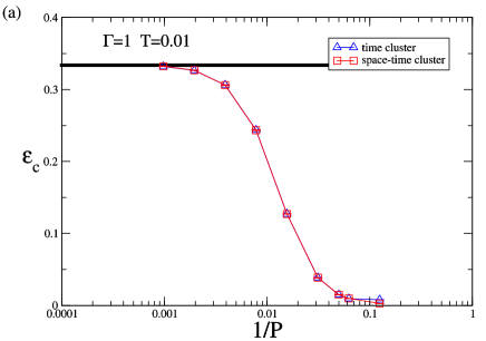
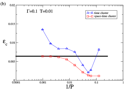
Figure 1: PIMC estimates of $\varepsilon_{\mathrm{c}}(\Gamma,T)$ in Eq. (7) at low temperature $k_{B}T=0.01$ and for two values of the transverse field, $\Gamma=1$ (a) and $\Gamma=0.1$ (b), as a function of the inverse number of Trotter slices $1/P$. The results are obtained for a given random instance of a chain of $L=256$ spins. The horizontal thick lines denote the exact $\varepsilon_{\mathrm{c}}(\Gamma,T)$ calculated from the Jordan-Wigner calculation. The simulation length is here $t_{\rm run}\lesssim 10^{8}\mbox{MCS}$. An initial $t_{\rm burn}$ MCS were discarded to ensure the equilibration of the Markov chain. The value of $t_{\rm burn}$ was chosen using Geweke’s diagnostic Brooks and Roberts (1998), while taking care to not discard more than 50% of the iterations.

Even more interesting is the outcome for $\Gamma=0.1<\Gamma_{c}$, see Fig. 1 (b). Here we see that the space-time (non-local) cluster moves correctly reproduce the exact $P\to\infty$ value, with the usual Trotter-error bias. However, the time-cluster moves (local in space) completely miss the exact target: as $P$ increases, the PIMC value first seems to move towards the exact one, up to roughly $P_{*}\sim 32\div 64$, but than strongly overshoots the target and shows deviations as large as a 100% error for the highest $P=1024$. This implies that the time cluster moves are unable to correctly sample the correct distribution, especially at relatively large $P$, even with quite long simulation times of order $t_{\rm run}\sim 10^{8}\,\mbox{MCS}$. The fact that a large-$P$ Trotter sampling is definitely non-trivial is well known for PIMC in continuous systems, see for instance Ref. Brualla et al., 2004. The time cluster moves are, however, the only candidate moves for PIMC in frustrated systems, where space-time cluster moves cannot be employed; they are also a quite natural implementation of a “physical” single-spin-flip dynamics.

III.2 PIMC-SQA compared to coherent QA

We now turn to the SQA dynamics. As done in previous studies Santoro et al. (2002); Martoňák et al. (2002); Heim et al. (2015), we use a protocol in which $\Gamma$ is linearly reduced to zero as a function of the Monte Carlo time. More precisely, we start from $\Gamma(0)=2.5$ and perform a preliminary equilibration of the system. We then reduce $\Gamma(t)$ at each MCS in such a way that $\Gamma(\tau)=0$, where $t$ is the time in MCS units and $\tau$ the total annealing time:

$$\Gamma(t)=\Gamma(0)\left(1-\frac{t}{\tau}\right)\;.$$ (10)

Notice that, in our choice, we reduce $\Gamma$ at each MCS, by a rather small quantity $\Delta\Gamma=\Gamma(0)/\tau$, rather than implementing a staircase with $N_{\Gamma}$ MCS at each of the $\tau/N_{\Gamma}$ values of $\Gamma$: the results are essentially equivalent. Let us consider, as a warm up, the ordered case $J_{i}=J$, where we set $J=1$ to be our energy unit. The coherent QA dynamics, here, is well known to produce a Kibble-Zurek Kibble (1980); Zurek (1996); Polkovnikov et al. (2011) decrease of the residual energy $\varepsilon_{\mathrm{res}}(\tau)\sim\tau^{-1/2}$. The SQA estimate, calculated from the Trotter replica average

$$\varepsilon_{\mathrm{res}}^{\mathrm{\scriptscriptstyle avg}}(\tau)=\frac{1}{L}\sum_{i=1}^{L-1}J_{i}\,\Big{(}1-\frac{1}{P}\sum_{k=1}^{P}S_{i}^{k}S_{i+1}^{k}\Big{)}\;,$$ (11)

at the final configuration $\{S_{i}^{k}\}$, averaged over many repetitions of the SQA run, is shown in Fig. 2 for the time cluster moves. Quite remarkably, the behaviour of $\varepsilon_{\mathrm{res}}^{\mathrm{\scriptscriptstyle avg}}(\tau)$ is well compatible with the KZ coherent behaviour, with the large $\tau$ deviations likely due to finite-size effects. We have verified that such KZ scaling would not be captured by using a SQA dynamics based on non-local (space-time) cluster moves.

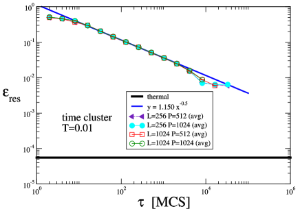
Figure 2: Test for Kibble-Zurek behaviour, $\varepsilon_{\mathrm{res}}(\tau)\sim\tau^{-1/2}$, in the ordered transverse-field Ising model. SQA is here implemented with SW time cluster moves at $T=0.01$. The horizontal thick line denotes the equilibrium thermal value of $\varepsilon_{\mathrm{c}}(\Gamma=0,T=0.01)$.

The natural question is whether this agreement survives also in the disordered case.

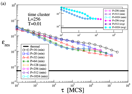
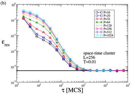
Figure 3: Residual energy at end of the SQA schedule as a function of the annealing time for various values of $P$ and a fixed disorder realization. The quantity we plot is $\varepsilon_{\mathrm{res}}^{\mathrm{\scriptscriptstyle min}}(\tau)$, see Eq. (12), except in the inset, where $\varepsilon_{\mathrm{res}}^{\mathrm{\scriptscriptstyle avg}}(\tau)$ is also shown.

We start by showing the results obtained, in the same spirit of the SQA numerics presented in Refs. Santoro et al., 2002; Martoňák et al., 2002; Heim et al., 2015, by considering the Trotter slice $k_{\star}$ that realizes the minimum classical energy value for the residual energy:

$$\varepsilon_{\mathrm{res}}^{\mathrm{\scriptscriptstyle min}}(\tau)=\frac{1}{L}\sum_{i=1}^{L-1}J_{i}\,\Big{(}1-S_{i}^{k_{\star}}S_{i+1}^{k_{\star}}\Big{)}\;,$$ (12)

for a given random instance of a chain with $L=256$ sites and $J_{i}\in[0,1]$. In Fig. 3(a) we show SQA data obtained for various $P$ with the SW time cluster moves. Notice the strong similarity with the SQA data shown in Ref. Santoro et al., 2002 and, in particular, with Fig. 3A of Ref. Heim et al., 2015, obtained for a two-dimensional frustrated Ising glass: this shows that, quite likely, the phenomena observed are due to disorder, rather than to a truly complex frustrated landscape. Notice also that, within an optimization framework, the optimal choice of $P$ is not $P\to\infty$, but rather $P_{\mathrm{\scriptscriptstyle min}}\sim 32$, as indeed empirically found in Ref. Santoro et al., 2002. As pointed out in Ref. Heim et al., 2015, these results raise doubts whether any possible advantage of SQA over plain SA might be lost in the proper quantum limit $P\to\infty$. Figure 3(b) shows that the SQA results obtained with the SW space-time cluster moves behave in a completely different way: they quickly converge to the expected thermal average $\varepsilon_{\mathrm{c}}(\Gamma=0,T=0.01)$. This simply tells that the SQA results are highly sensitive to the type of MC moves one adopts, as perhaps expected: most likely, the space-time cluster non-local moves have little to do with any physical dynamics, as we will further comment on in the following.

Returning to the time cluster SQA results, we re-plot them in the inset of Fig. 3(a) for the largest $P$, to highlight the fact that the $P\to\infty$ limit is indeed reached as soon as $P\geq 256$. Here, the two sets of data shown are $\varepsilon_{\mathrm{res}}^{\mathrm{\scriptscriptstyle min}}(\tau)$, the optimal Trotter-slice value in Eq. (12), against the proper “quantum average” $\varepsilon_{\mathrm{res}}^{\mathrm{\scriptscriptstyle avg}}(\tau)$ in Eq. (11), which shows a much smoother and monotonic behaviour: notice that the two curves approach each other for the largest $\tau$ investigated. This witnesses the fact that, for these largest $\tau$, the quantum fluctuations — i.e. the fluctuations along the Trotter-time direction — seem to play no role towards the end of the annealing.

But the question remains: is there any physics that we can learn from the time cluster SQA dynamics in the disordered case? The first tests we have performed consist in monitoring the dynamics of $\epsilon_{\mathrm{res}}(t,\tau)$, for given $\tau$, versus $t$, both for the QA unitary evolution and the SQA dynamics. Indeed, since each $t$ is univocally associated to a value of $\Gamma(t)$, we can equivalently plot the SQA results, averaged over many repetitions of the Monte Carlo dynamics, versus $\Gamma$. Figure 4(a) shows the results for three values of $\tau$, with the SQA results denoted by points. Here we find a surprising result: the SQA with time-cluster moves visits configurations which are essentially equilibrium configurations, but at an effective temperature $T_{\rm eff}(\tau)$, which depends on the total annealing time $\tau$. More precisely, we have verified that the following Ansatz for the dynamical residual energy holds:

$$\epsilon_{\mathrm{res}}(t,\tau)=\varepsilon_{\mathrm{c}}(\Gamma(t),T_{\rm eff}(\tau))\;,$$ (13)

where the corresponding equilibrium values of $\varepsilon_{\mathrm{c}}(\Gamma,T_{\rm eff})$, with $T_{\rm eff}$ obtained by fitting the numerical points, are shown by dashed lines in Fig. 4(a). Even more remarkably, the same Ansatz also holds, on the same disordered instance, for the coherent QA dynamics, performed integrating through a $4^{\rm th}$-order Runge-Kutta algorithm the BdG equations Caneva et al. (2007); Zanca and Santoro (2016) for the free-fermion Jordan-Wigner mapping, see Fig. 4(b).

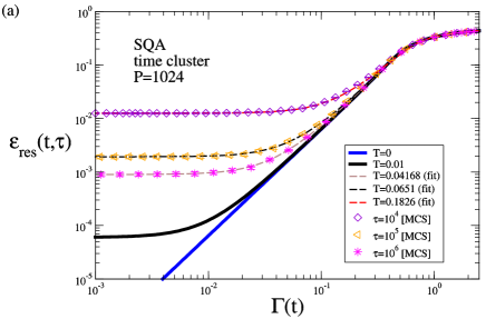
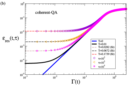
Figure 4: Test of the dynamical Ansatz in Eq. (13) for the time-cluster SQA dynamics (a) and the coherent QA dynamics (b), for the same disorder realization of Fig. 3. The numerical data for $\epsilon_{\mathrm{res}}(t,\tau)$ are shown by points, for different $\tau$, at the corresponding value for $\Gamma(t)$, while the fits with the equilibrium $\varepsilon_{\mathrm{c}}(\Gamma,T_{\rm eff}(\tau))$ are shown by dashed lines. For comparison, the exact equilibrium values for $\varepsilon_{\mathrm{c}}(\Gamma,T=0.01)$ and $\varepsilon_{\mathrm{c}}(\Gamma,T=0)$ are also shown by thick solid lines.

We might go on and compare the corresponding $T_{\rm eff}(\tau)$ obtained for the two dynamics. However, since $\varepsilon_{\mathrm{res}}(\tau)=\varepsilon_{\mathrm{c}}(\Gamma=0,T_{\rm eff}(\tau))$, due to the validity of the Ansatz (13), we can equivalently compare the results obtained for $\varepsilon_{\mathrm{res}}(\tau)$ in the two cases.

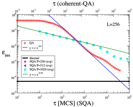
Figure 5: The residual energy $\varepsilon_{\mathrm{res}}(\tau)$ at the end of the annealing for the same disorder realization of Fig. 3. The stars show the coherent-QA results vs $\tau$ (upper abscissa axis) while the other symbols refer to the SQA results (the same data shown in the inset of Fig. 3(a)). The equilibrium thermal value $\varepsilon_{\mathrm{c}}(\Gamma=0,T=0.01)$ is shown by a thick horizontal line.

Figure 5 shows such a comparison. The solid symbols show the SQA results for $\varepsilon_{\mathrm{res}}^{\mathrm{\scriptscriptstyle avg}}(\tau)$ in Eq. (11), already reported in the inset of Fig. 3(a), while the stars show the coherent-QA $\varepsilon_{\mathrm{res}}(\tau)$. Quite evidently, both plots show an intermediate power-law part which, however, shows markedly different power-law exponents in the two cases, $\sim\tau^{-0.9}$ for coherent-QA compared to $\sim\tau^{-0.35}$ for SQA: hence, no linear scaling of the physical against the MC time can ever make the two results consistent. The situation does not improve for large $\tau$, where it is known Dziarmaga (2006); Caneva et al. (2007) that, in the thermodynamic limit, the coherent-QA results would display a logarithmic slow-down Santoro et al. (2002), $\varepsilon_{\mathrm{res}}(\tau)\sim[\log(\gamma\tau)]^{-\xi}$, with $\xi>2$: the data for $L=265$ evidently still suffer from finite-size effects which prevent from appreciating such a subtle logarithmic slow-down; nevertheless, they clearly depart from the intermediate-$\tau$ data by staying above the power-law $\sim\tau^{-0.9}$. On the contrary, the SQA data depart from their intermediate-time power-law $\sim\tau^{-0.35}$ from below, but then show a final slow-down of difficult interpretation.

IV Conclusions

We have investigated some aspects of the dynamics behind Simulated Quantum Annealing (SQA), specifically its Path-Integral Monte Carlo (PIMC) implementation, through a detailed analysis of PIMC-SQA on a transverse-field random Ising spin chain, where exact equilibrium and coherent-QA results are easily obtained.

Due to the absence of frustration, we were also able to compare results obtained with two types of Monte Carlo (MC) moves, a local-in-space Swendsen-Wang cluster move limited to the imaginary-time direction, against space-time (non-local) SW cluster moves, which provides an extremely fast Monte Carlo dynamics. The results show that the choice of the MC moves is of course crucial, but that fast non-local cluster moves have nothing to do with any physical dynamics, which is better mimicked by local spin-flip moves.

Concerning the latter more physical choice, we have verified that the expected Kibble-Zurek behaviour $\varepsilon_{\mathrm{res}}(\tau)\sim\tau^{-1/2}$ is well reproduced by SQA in the ordered case. In presence of disorder, however, we found that equilibrium thermodynamical PIMC simulations at finite $T$ show a sampling problem emerging, for large $P$, below the critical point $\Gamma<\Gamma_{c}$ and at low temperatures. The consequences of such a sampling problem on the SQA dynamics are a priori not obvious. Interestingly, we found that the time-dependent residual energy $\epsilon_{\mathrm{res}}(t,\tau)$ shows features that are shared also by the coherent-QA Schrödinger dynamics, i.e., $\epsilon_{\mathrm{res}}(t,\tau)$ is perfectly described by the (instantaneous) equilibrium value of $\varepsilon_{\mathrm{c}}(\Gamma(t),T_{\rm eff}(\tau))$ at an effective temperature $T_{\rm eff}(\tau)$ which depends on the annealing time $\tau$. Nevertheless, the SQA results for the residual energy $\varepsilon_{\mathrm{res}}(\tau)$ appear to be unrelated, in presence of disorder, with the corresponding coherent-QA results.

Several points still deserve a discussion. One might question the relevance of a comparison of SQA at a finite (low) $T$ against QA results which assume a coherent Schrödinger evolution in absence of any external bath. On the practical side, we might add that while a coherent-QA evolution is here quite easy to perform — you just have to integrate $2L\times 2L$ BdG equations for the Jordan-Wigner fermions — the physical dissipative dynamics of a random Ising chain is still a problem which we do not know how to efficiently and reliably tackle. More to the point, however, we can give arguments which are based on our current understanding of the role of dissipation in the QA dynamics of the ordered Ising chain Patanè et al. (2008, 2009); Arceci et al. (2018). As indeed shown in Ref. Arceci et al., 2018, and perhaps easy to argue about, dissipation has very little effect at small and intermediate annealing times $\tau$, which implies that the different power-law behaviour displayed in Fig. 5 would likely not be influenced by the presence of a bath. For large $\tau$, on the other hand, dissipation tends to drive the system closer to a thermal steady state, which likely results in a larger residual energy, $\varepsilon_{\mathrm{res}}^{\rm diss}(\tau)>\varepsilon_{\mathrm{res}}(\tau)$, due to thermal defects generation. Hence, again, it is unlikely that the effect of a thermal bath at temperature $T$ would lead to a closer agreement between SQA and a physical open quantum system dynamics.

A few comments deserves also the largely accepted viewpoint that the time-continuum limit $P\to\infty$ is crucial for a comparison against real QA hardware devices. While there is no question on the fact that, as pointed out in Ref. Heim et al., 2015, a correct quantum mechanical treatment does require the limit $P\to\infty$, this by itself does not guarantee that the resulting SQA dynamics is physical, as we have shown in this paper.

The typical “slow-down” that SQA data with $P\to\infty$ tend to show for large $\tau$ should also not necessarily be taken to imply that there is no quantum speed-up of any type against classical Simulated Annealing (SA). Indeed, based on theoretical arguments Santoro et al. (2002), a coherent-QA is expected to show some improvement in the exponent of the logarithmic scaling, $\varepsilon_{\mathrm{res}}(\tau)\sim[\log(\gamma\tau)]^{-\xi}$, against competing SA strategies: this improvement has been indeed verified on random Ising chains Caneva et al. (2007); Suzuki (2009); Zanca and Santoro (2016) and on infinitely connected $p$-spin Ising ferromagnets Wauters et al. (2017). Moreover, quite remarkably, non-convex optimization problems are known Baldassi and Zecchina (2018) in which SQA, with the $P\to\infty$ limit properly taken, is definitely much more efficient than its classical SA counterpart.

References

- Finnila et al. (1994) A. B. Finnila, M. A. Gomez, C. Sebenik, C. Stenson, and J. D. Doll, Chem. Phys. Lett. 219, 343 (1994).
- Kadowaki and Nishimori (1998) T. Kadowaki and H. Nishimori, Phys. Rev. E 58, 5355 (1998).
- Brooke et al. (1999) J. Brooke, D. Bitko, T. F. Rosenbaum, and G. Aeppli, Science 284, 779 (1999).
- Santoro et al. (2002) G. E. Santoro, R. Martoňák, E. Tosatti, and R. Car, Science 295, 2427 (2002).
- Santoro and Tosatti (2006) G. E. Santoro and E. Tosatti, J. Phys. A: Math. Gen. 39, R393 (2006).
- Farhi et al. (2001) E. Farhi, J. Goldstone, S. Gutmann, J. Lapan, A. Lundgren, and D. Preda, Science 292, 472 (2001).
- Kirkpatrick et al. (1983) S. Kirkpatrick, J. C. D. Gelatt, and M. P. Vecchi, Science 220, 671 (1983).
- Harris et al. (2010) R. Harris et al., Phys. Rev. B 82, 024511 (2010).
- Johnson et al. (2011) M. W. Johnson et al., Nature 473, 194 (2011).
- Denchev et al. (2016) V. S. Denchev, S. Boixo, S. V. Isaksov, N. Ding, R. Babbush, V. Smelyanskiy, and J. Martinis, Phys. Rev. X 6, 031015 (2016).
- Lanting et al. (2014) T. Lanting et al., Phys. Rev. X 4, 021041 (2014).
- Boixo et al. (2013) S. Boixo, T. Albash, F. M. Spedalieri, N. Chancellor, and D. A. Lidar, Nat. Commun. 4, 2067 (2013).
- Dickson et al. (2013) N. G. Dickson et al., Nat. Commun. 4, 1903 (2013).
- Boixo et al. (2014) S. Boixo, T. F. Rønnow, S. V. Isaksov, Z. Wang, D. Wecker, D. A. Lidar, J. M. Martinis, and M. Troyer, Nat. Phys. 10, 218 (2014).
- Rønnow et al. (2014) T. F. Rønnow, Z. Wang, J. Job, S. Boixo, S. V. Isakov, D. Wecker, J. M. Martinis, D. A. Lidar, and M. Troyer, ArXiv e-prints (2014), arXiv:1401.2910 .
- Muthukrishnan et al. (2016) S. Muthukrishnan, T. Albash, and D. A. Lidar, Phys. Rev. X 6, 031010 (2016).
- Albash and Lidar (2018) T. Albash and D. A. Lidar, Phys. Rev. X 8, 031016 (2018).
- Hormozi et al. (2017) L. Hormozi, E. W. Brown, G. Carleo, and M. Troyer, Phys. Rev. B 95, 184416 (2017).
- Susa et al. (2017) Y. Susa, J. F. Jadebeck, and H. Nishimori, Phys. Rev. A 95, 042321 (2017).
- Amin and Averin (2008) M. H. S. Amin and D. V. Averin, Phys. Rev. Lett. 100, 197001 (2008).
- Arceci et al. (2017) L. Arceci, S. Barbarino, R. Fazio, and G. E. Santoro, Phys. Rev. B 96, 054301 (2017).
- Arceci et al. (2018) L. Arceci, S. Barbarino, D. Rossini, and G. E. Santoro, ArXiv e-prints (2018), arXiv:1804.04251 .
- Becca and Sorella (2017) F. Becca and S. Sorella, Quantum Monte Carlo approaches for correlated systems (Cambridge Univ. Press, 2017).
- Ceperley (1995) D. M. Ceperley, Rev. Mod. Phys. 67, 279 (1995).
- Martoňák et al. (2002) R. Martoňák, G. E. Santoro, and E. Tosatti, Phys. Rev. B 66, 094203 (2002).
- Suzuki (1976) M. Suzuki, Prog. Theor. Phys. 56, 1454 (1976).
- Boixo et al. (2014) S. Boixo, T. F. Rønnow, S. V. Isakov, Z. Wang, D. Wecker, D. A. Lidar, J. M. Martinis, and M. Troyer, Nat. Phys. 10, 218 (2014).
- Isakov et al. (2016) S. V. Isakov, G. Mazzola, V. N. Smelyanskiy, Z. Jiang, S. Boixo, H. Neven, and M. Troyer, Phys. Rev. Lett. 117, 180402 (2016).
- Mazzola et al. (2017) G. Mazzola, V. N. Smelyanskiy, and M. Troyer, Phys. Rev. B 96, 134305 (2017).
- Andriyash and Amin (2017) E. Andriyash and M. H. Amin, ArXiv e-prints (2017), arXiv:1703.09277 .
- Inack et al. (2018) E. M. Inack, G. Giudici, T. Parolini, G. Santoro, and S. Pilati, Phys. Rev. A 97, 032307 (2018).
- Albash et al. (2015a) T. Albash, I. Hen, F. M. Spedalieri, and D. A. Lidar, Phys. Rev. A 92, 062328 (2015a).
- Albash et al. (2015b) T. Albash, T. Rønnow, M. Troyer, and D. Lidar, EPJ ST 224, 111 (2015b).
- Heim et al. (2015) B. Heim, T. F. Rønnow, S. V. Isakov, and M. Troyer, Science 348, 215 (2015).
- Baldassi and Zecchina (2018) C. Baldassi and R. Zecchina, PNAS 115, 1457 (2018).
- Lieb et al. (1961) E. Lieb, T. Schultz, and D. Mattis, Ann. Phys. 16, 407 (1961).
- Young and Rieger (1996) A. P. Young and H. Rieger, Phys. Rev. B 53, 8486 (1996).
- Swendsen and Wang (1987) R. H. Swendsen and J.-S. Wang, Phys. Rev. Lett. 58, 86 (1987).
- Caneva et al. (2007) T. Caneva, R. Fazio, and G. E. Santoro, Phys. Rev. B 76, 144427 (2007).
- Kibble (1980) T. W. B. Kibble, Phys. Rep. 67, 183 (1980).
- Zurek (1996) W. H. Zurek, Phys. Rep. 276, 177 (1996).
- Polkovnikov et al. (2011) A. Polkovnikov, K. Sengupta, A. Silva, and M. Vengalattore, Rev. Mod. Phys. 83, 863 (2011).
- Suzuki (2009) S. Suzuki, JSTAT , P03032 (2009).
- Zanca and Santoro (2016) T. Zanca and G. E. Santoro, Phys. Rev. B 93, 224431 (2016).
- Dziarmaga (2006) J. Dziarmaga, Phys. Rev. B 74, 064416 (2006).
- Wolff (1989) U. Wolff, Phys. Rev. Lett. 62, 361 (1989).
- Fisher (1995) D. S. Fisher, Phys. Rev. B 51, 6411 (1995).
- Brooks and Roberts (1998) S. P. Brooks and G. O. Roberts, Statistics and Computing 8, 319 (1998).
- Brualla et al. (2004) L. Brualla, K. Sakkos, J. Boronat, and J. Casulleras, J. Chem. Phys. 121, 636 (2004).
- Patanè et al. (2008) D. Patanè, A. Silva, L. Amico, R. Fazio, and G. E. Santoro, Phys. Rev. Lett. 101, 175701 (2008).
- Patanè et al. (2009) D. Patanè, A. Silva, L. Amico, R. Fazio, and G. E. Santoro, Phys. Rev. B 80, 2009 (2009).
- Wauters et al. (2017) M. M. Wauters, R. Fazio, H. Nishimori, and G. E. Santoro, Phys. Rev. A 96, 022326 (2017).