A Low-Complexity Detection Algorithm For Uplink Massive MIMO Systems Based on Alternating Minimization

Abstract

In this paper, we propose an algorithm based on the Alternating Minimization technique to solve the uplink massive MIMO detection problem. The proposed algorithm is specifically designed to avoid any matrix inversion and any computations of the Gram matrix at the receiver. The algorithm provides a lower complexity compared to the conventional MMSE detection technique, especially when the total number of user equipment (UE) antennas (across all users) is close to the number of base station (BS) antennas. The idea is that the algorithm re-formulates the maximum likelihood (ML) detection problem as a sum of convex functions based on decomposing the received vector into multiple vectors. Each vector represents the contribution of one of the transmitted symbols in the received vector. Alternating Minimization is used to solve the new formulated problem in an iterative manner with a closed form solution update in every iteration. Simulation results demonstrate the efficacy of the proposed algorithm in the uplink massive MIMO setting for both coded and uncoded cases.

I Introduction

Massive multiple-input multiple-output (MIMO) is one of the most promising techniques for the 5th Generation (5G) networks due to its potential for enhancing throughput, spectra efficiency, and energy efficiency [1], [2]. Massive MIMO requires the BS to be equipped with arrays of hundreds of antennas to serve tens of user terminals with single or multiple antennas.

Theoretical results of massive MIMO show that linear detectors such as zero forcing (ZF) and minimum mean square error (MMSE) can achieve optimum performance under the favorable propagation conditions [3]. The favorable propagation condition means that the number of BS antennas grows very large compared to the number of UE antennas, which leads to the column-vectors of the propagation matrix to be asymptotically orthogonal. As a result of this orthogonality, the ZF and MMSE detectors can be implemented with simple diagonal inversions [4].

The current practical number of the BS antennas in massive MIMO systems is in the order of tens to a hundred. This is far from the theoretical limit that leads to the orthogonality mentioned above [4]. Therefore, the linear detectors still need to perform a matrix inversion for the signal detection of the uplink massive MIMO system, which entails extensive computational complexity [5]. Neumann series expansion, Cholesky decomposition, and successive over-relaxation techniques are proposed in the literature to reduce the complexity of the matrix inversion process in the MMSE detector [6] [7]. These approaches require a lower computational complexity than the exact matrix inversion while delivering near-optimal results only for theoretical massive MIMO configurations, that is, when the ratio between the number of BS antennas and the number of single antenna users is large enough (e.g., $\geq 16$) [8]. In realistic massive MIMO scenarios where this ratio is small, [8] indicates that a large truncation order is required for Neumann series expansion technique which makes the computational complexity higher than the exact matrix inversion operations. Moreover, implementing these approximations significantly deteriorate performance as compared to the exact MMSE performance [6].

In this letter we present a novel formulation of a low complexity iterative algorithm based on Alternating Minimization, referred to as AltMin. This algorithm provides similar bit error rate (BER) performance to the exact matrix inverted MMSE technique, with one order less complexity.

The proposed algorithm approximates ML detection problem as a sum of convex functions based on decomposing the received vector into multiple vectors. Each vector represents the contribution of one of the transmitted symbols in the received vector. Then, Alternating Minimization is used to solve the new formulated problem in an iterative manner with a closed form solution update in every iteration that does not require any matrix inversion or any matrix multiplications.

Although there are several algorithms presented in the literature for the uplink massive MIMO detection problem, the key contributions include the following: (1) the re-formulation of the problem is novel, (2) the alternating minimization used to solve the proposed formulation has a closed form expression update at every iteration. The algorithm avoids any matrix inversion and any computations of the Gram matrix (i.e., $\textbf{H}^{H}\textbf{H}$). Thus, the proposed approach is low-complexity and has been shown empirically to perform better than the considered baseline.

II System Model and Problem Formulation

II-A System Model

Consider the uplink data detection in a multi-user (MU) massive MIMO system with $N_{r}$ BS antennas and $N_{t}$ UE antennas. The vector $\tilde{\textbf{x}}=(\tilde{x}_{1},\tilde{x}_{2},\dots,\tilde{x}_{N_{t}})^{T}\in\mathbb{C}^{N_{t}\times 1}$ represents the complex transmitted signal, where $x_{k}$ is the transmitted symbol for user $k$ with $E{|\tilde{x}_{i}|^{2}}=1,\forall i$. Each user transmits symbols over a flat fading channels and the signals are demodulated and sampled at the receiver. The vector $\tilde{\textbf{y}}=(\tilde{y}_{1},\tilde{y}_{2},\dots,\tilde{y}_{N_{r}})^{T}\in\mathbb{C}^{{N_{r}}\times 1}$ represents the complex received signal, and the channel matrix $\tilde{\textbf{H}}\in\mathbb{C}^{{N_{r}}\times N_{t}}$ can be represented as $(\tilde{\textbf{h}}_{1},\tilde{\textbf{h}}_{2},\dots,\tilde{\textbf{h}}_{N_{t}})$, where $\tilde{\textbf{h}}_{i}=(\tilde{h}_{1,i},\tilde{h}_{2,i},...,\tilde{h}_{N_{r},i})^{T}\in\mathbb{C}^{{N_{r}}\times 1}$, and $\tilde{h}_{m,n}$ is the fading channel gain from transmit antenna $n$ to the receive antenna $m$ that is assumed to be i.i.d. (independent and identically distributed) complex Gaussian random variables with zero mean and unit variance, i.e., $\tilde{h}_{m,n}\sim\mathcal{CN}(0,1)$. The system can be modeled as; $\tilde{\textbf{{y}}}=\tilde{\textbf{{H}}}\tilde{\textbf{{x}}}+\tilde{\textbf{{v}}}$, where the $\tilde{\textbf{v}}=(\tilde{v}_{1},\tilde{v}_{2},,\tilde{v}_{N_{r}})^{T}\in\mathbb{C}^{{N_{r}}\times N_{t}}$ is the complex additive white Gaussian noise (AWGN) vector whose elements are mutually independent with zero mean and variance $\sigma^{2}_{v}$. The corresponding real-valued system model is $\textbf{{y}}=\textbf{{H}}\textbf{{x}}+\textbf{{v}}$ [9], [10], where $\textbf{{x}}\in\mathbb{R}^{2N_{t}\times 1}$, $\textbf{{y}}\in\mathbb{R}^{2N_{r}\times 1}$, $\textbf{{v}}\in\mathbb{R}^{2N_{r}\times 1}$, and $\textbf{{H}}\in\mathbb{R}^{2N_{r}\times 2N_{t}}$. The equivalent ML detection problem of the real model can be written in the form $\widehat{{\textbf{x}}}=\underset{{{\textbf{x}}\in\chi^{2N_{t}}}}{\text{argmin}}\parallel{{\textbf{y}}}-{{\textbf{H}}}{{\textbf{x}}}\parallel_{2}^{2}$, where $\chi=\frac{1}{\Gamma}\{-\sqrt{\textit{M}}+1,..,-1,1,...,\sqrt{\textit{M}}-1\}$, M is the constellation size, and $\frac{1}{\Gamma}$ is for normalization factor.

II-B Problem Formulation

First, we decompose the received vector y into a linear combination of vectors so that $\textbf{y}=\sum_{i=1}^{2N_{t}}{\textbf{y}_{i}}$, where $\textbf{y}_{i}$ represents the contribution of the $i$-th transmitted symbol in the received vector. The element wise representation of the decomposed received vector is:

$\begin{bmatrix}y^{(1)}\\ .\\ .\\ y^{(k)}\\ .\\ .\\ y^{(2N_{r})}\\ \end{bmatrix}=\begin{bmatrix}y_{1}^{(1)}\\ .\\ .\\ y_{1}^{(k)}\\ .\\ .\\ y_{1}^{(2N_{r})}\\ \end{bmatrix}+\cdots+\begin{bmatrix}y_{i}^{(1)}\\ .\\ .\\ y_{i}^{(k)}\\ .\\ .\\ y_{i}^{(2N_{r})}\\ \end{bmatrix}+\cdots+\begin{bmatrix}y_{2N_{t}}^{(1)}\\ .\\ .\\ y_{2N_{t}}^{(k)}\\ .\\ .\\ y_{2N_{t}}^{(2N_{r})}\\ \end{bmatrix}$

where $y_{i}^{(k)}$ represents the $k$-th element of the decompose vector $\textbf{y}_{i}$. Thus, the $k$-th element of the real-valued received vector y can be represented as ${y}^{(k)}=\sum_{i=1}^{2N_{t}}{{y}_{i}^{(k)}}$, $k=1,\dots,2N_{r}$. Let $\textbf{h}_{i}$ be the $i$-th column of the real-valued channel matrix H. Now, we relax the non-convexity constraint on the feasible set $\chi$, and approximate the ML problem based on the above decomposition as follows:

$$\underset{{x_{i}},\textbf{y}_{i}\forall i}{\text{argmin}}\sum_{i=1}^{2N_{t}}\parallel{{\textbf{y}_{i}}}-{{\textbf{h}_{i}}}{{{x}_{i}}}\parallel_{2}^{2}\,\,\,\,\,\text{subject to}$$ (1)

$$\sum_{i=1}^{2N_{t}}{{y}_{i}}^{(k)}={y}^{(k)},\forall k=1,\cdots,2N_{r}$$ (2)

$$-l\leq{x}_{i}\leq l,\forall i=1,\cdots,2N_{t}$$ (3)

Where $l=\frac{1}{\Gamma}(\sqrt{\textit{M}}-1)$. The objective function in (1) is a sum of separable terms, each of which is a function of only one symbol and its contribution in the received vector. In the next section, we use AltMin to solve the proposed formulation.

III Proposed Algorithm

The optimization problem (1)-(3) is strictly and jointly convex with respect to x and ${\bf{\cal Y}}$ where, ${\bf{\cal Y}}=\big{\{}\textbf{y}_{i}\forall i:i\in\{1,2,\cdots,2N_{t}\}\big{\}}$. Moreover, there is no common constraint that combines both x and ${\bf{\cal Y}}$. Therefore, in order to efficiently solve this problem, we first decompose it into the following two subproblems:

• Given x, we obtain ${\bf{\cal Y}}$ by solving

  $$\underset{\textbf{y}_{i}}{\text{argmin}}\sum_{i=1}^{2N_{t}}\parallel{{\textbf{y}_{i}}}-{{\textbf{h}_{i}}}{x_{i}}\parallel_{2}^{2}\quad\text{subject to}\,\eqref{eq: 7c1}$$ (4)

• Given ${\bf{\cal Y}}$, we obtain x by solving

  $$\underset{x_{i}}{\text{argmin}}\sum_{i=1}^{2N_{t}}\parallel{{\textbf{y}_{i}}}-{{\textbf{h}_{i}}}{{x_{i}}}\parallel_{2}^{2}\quad\text{subject to}\,\eqref{eq: 7c2}$$ (5)

Then, we propose, AltMin, an iterative algorithm that alternatively solves (4) for ${\bf{\cal Y}}$ and (5) for x given the other. Note that the respective Karush-Kuhn-Tucker (K.K.T) conditions [11] of the above two subproblems form the complete set of the K.K.T. conditions for the original problem.

III-A Solving the subproblem (4)

The Lagrangian function of (4) can be written as:

$$\mathcal{L}=\sum_{i=1}^{2N_{t}}\parallel{{\textbf{y}_{i}}}-{{\textbf{h}_{i}}}{x_{i}}\parallel_{2}^{2}+\sum_{k=1}^{2N_{r}}\lambda^{k}(y^{(k)}-\sum_{i=1}^{2N_{t}}{y_{i}}^{(k)})$$ (6)

Therefore, by solving the above Lagrangian function, which is a function of $\lambda^{(k)}$ and $\textbf{y}_{i}$, we get the following closed form expression updates for every element of $\lambda^{(k)}$ and $y_{i}^{(k)}$:

$$\lambda^{(k)}=C\cdot\frac{1}{N_{t}}(y^{(k)}-\sum_{i=1}^{2N_{t}}h_{i}^{(k)}x_{i}),\forall k$$ (7)

$$y_{i}^{(k)}=h_{i}^{(k)}x_{i}+\lambda^{(k)}/2,\forall i,k$$ (8)

where $h_{i}^{(k)}$ represents the k-th element in column vector $\textbf{h}_{i}$, which corresponds to the $i^{\text{th}}$ column of the the real-valued channel matrix H. Note that in the update of $\lambda^{(k)}$, we introduce the scaling factor, $C$. We show in Section III-C that the proposed algorithm is optimal when $C=1$. However, we empirically find that when $C=N_{t}$, the number of iterations for convergence drops significantly, see Section IV-A.

III-B Solving the subproblem (5)

The objective function (5) is separable with respect to every element $x_{i}$ in the vector x, and no constraint combines the elements of x. Therefore, the update of the $i$-th element in the vector x reduces to solving the following subproblem.

$$\underset{x_{i}}{\text{argmin}}\sum_{k=1}^{2N_{r}}(y_{i}^{(k)}-h_{i}^{(k)}x_{i})^{2}\quad\text{subject to }~{}\eqref{eq: 7c2}$$ (9)

The corresponding Lagrangian function of  (9) is:

$$\mathcal{L}=\sum_{k=1}^{2N_{r}}(y_{i}^{(k)}-h_{i}^{(k)}x_{i})^{2}+\mu_{1}^{(i)}(l-x_{i})+\mu_{2}^{(i)}(l+x_{i})$$ (10)

Then, the following K.K.T. conditions [11] which are sufficient and necessary for the optimal solution to the convex optimization problem in (9) are:

$$2x_{i}\sum_{k=1}^{2N_{r}}{h_{i}^{(k)}}^{2}-2\sum_{k=1}^{2N_{r}}y_{i}^{(k)}h_{i}^{(k)}-\mu_{1}^{(i)}+\mu_{2}^{(i)}=0$$ (11)

$$\mu_{1}^{(i)}(l-x_{i})=0,\,\,\mu_{2}^{(i)}(l+x_{i})=0,\,\,\mu_{1}^{(i)},\mu_{2}^{(i)}\geq 0$$ (12)

In order to solve (11)-(12) for every element in the vector x, among the following $\{\mu_{1}^{(i)},\mu_{2}^{(i)},x_{i}\}$ choices, we choose the one that minimizes (9):

$$\mu_{1}^{(i)}=0,\text{ and }\mu_{2}^{(i)}=0\rightarrow x_{i}=\frac{\sum_{k=1}^{2N_{r}}y_{i}^{(k)}h_{i}^{(k)}}{\sum_{k=1}^{2N_{r}}{h_{i}^{(k)}}^{2}}$$ (13)

$$\mu_{1}^{(i)}=0,\text{ and }\mu_{2}^{(i)}\neq 0\rightarrow x_{i}=-l$$ (14)

$$\mu_{1}^{(i)}\neq 0,\text{ and }\mu_{2}^{(i)}=0\rightarrow x_{i}=l$$ (15)

Note, we exclude the choice $\mu_{1}^{(i)}\neq 0$, and $\mu_{2}^{(i)}\neq 0$ since $x_{i}$ cannot be equal to $-l$ and $l$ at the same time.

To obtain the optimal solution to the proposed optimization problem (1)-(3), AltMin solves (4) for ${\bf{\cal Y}}$ and (5) for x. To perform the algorithm, we initially set x to 0, and solve (4) to obtain the initial ${\bf{\cal Y}}$. With updated ${\bf{\cal Y}}$, we solve  (5) to update x. The proposed algorithm is summarized in Algorithm 1.

1:  1: Initilization

2:  $t=0$, $x_{i}=0\forall i$

3:  update $\lambda^{(k)}\forall k$ according to equation (7)

4:  update $y_{i}^{(k)}\forall i,k$ according to equation (8)

5:  $V^{(t)}=\sum_{i=1}^{2N_{t}}\parallel{{\textbf{y}_{i}}}-{{\textbf{h}_{i}}}{{x_{i}}}\parallel_{2}^{2}$

6:  $\delta=$ convergence tolerance

7:  $T=$ Maximum number of iterations

8:  2: Alternating Minimization:

9:  repeat

10:     $t\leftarrow t+1$

11:     update $x_{i}\forall i$ according to  (13)

12:     update $\lambda^{(k)}\forall k$ according to equation (7)

13:     update $y_{i}^{(k)}\forall i,k$ according to equation (8)

14:     $V^{(t)}=\sum_{i=1}^{2N_{t}}\parallel{{\textbf{y}_{i}}}-{{\textbf{h}_{i}}}{{x_{i}}}\parallel_{2}^{2}$

15:  until $|V^{(t)}-V^{(t-1)}|<\delta$ OR $t>T$

Algorithm 1 Proposed Algorithm

III-C Optimality of AltMin Algorithm in solving (1)-(3)

In order to show the optimality of the iterative algorithm (when $C=1$), we first give the following lemma.

Lemma 1.

Given x, the optimal ${\bf{\cal Y}}$ for the problem (4) is unique. Similarly, given ${\bf{\cal Y}}$, the optimal x to (5) is unique.

Proof.

This lemma can be obtained by verifying the strict convexity of (1)-(3) with respect to x given ${\bf{\cal Y}}$, and with respect to ${\bf{\cal Y}}$ given x. ∎

Theorem 1.

AltMin Algorithm converges, and (${\bf{\cal Y}}$, x) is optimal to (1)-(3).

Proof.

We use the result in [12] to show the optimality and convergence of alternating minimization, which requires us to show five conditions. The first condition is satisfied since the constraints do not have both variables together and are linear functions. The second condition indicates that the objective is a continuously differentiable convex function which also holds as the Hessian matrix of the objective function is positive semidefinite. The third and the fourth conditions are satisfied since the objective function is uniformly Lipschitz continuous with respect to each of the variable. The fifth condition is that the two sub-problems have minimizers which holds by Lemma 1. This proves the result as in the statement of the Theorem. ∎

III-D Complexity Analysis of AltMin

The update of ${\bf{\cal Y}}$ has a complexity of $O(N_{t}N_{r})$, while the update of x has a complexity of $O(N_{t})$. The AltMin algorithm performs $T$ iterations between these updates before converging to the optimal solution. Therefore, the overall complexity of AltMin in solving (1)-(3) is $O(TN_{t}N_{r})$, which is notably lower than $O(N_{t}^{3})$ of MMSE for large $N_{t}$, as demonstrated in Section IV.

IV Numerical Results

Numerical results for coded and uncoded uplink massive MIMO systems in a block flat fading channel is presented. We assume perfect knowledge of the channel state information at the receiver. QPSK modulation is considered for demonstration; however, the proposed algorithm can be extended for higher QAM modulations in a straightforward manner. The performance and computational complexity of the proposed algorithm is compared with the linear MMSE detector.

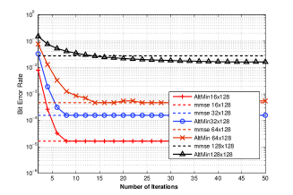
Figure 1: BER performance versus AltMin Iterations at SNR=12 dB

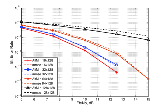
Figure 2: BER performance comparison for different massive MIMO configurations

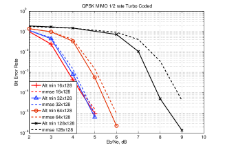
Figure 3: 1/2 Turbo coded BER performance of QPSK

IV-A Number of AltMin Iterations

In this simulation experiment, we examine the number of iterations required by the AltMin algorithm such that the BER performance of both the proposed algorithm and the MMSE technique are equal, for various massive MIMO configurations. We fix convergence tolerance $\delta$ at $10^{-3}$, while the maximum number of iterations $T$ is changing in a step size of 2. We also set the initial guess of x in the AltMin algorithm to zeros, and $C=N_{t}$ in the update of $\lambda^{(k)}$ in (7).

Fig. 3 shows BER performance versus maximum number of iterations for $N_{t}\times N_{r}=16\times 128,32\times 128,64\times 128$, and $128\times 128$ configurations, at SNR=12 dB. It can be noticed that the larger the ratio $\frac{N_{r}}{N_{t}}$ is, the smaller the number of iterations is required by AltMin to reach the MMSE performance. For example, 8 iterations is required for $16\times 128$ configuration, while 15 iterations is required for $128\times 128$ configuration. This results show that, on the average, to reach the MMSE performance, the required number of iterations, $T$, is much smaller than $N_{t}$. Consequently, the complexity of the proposed algorithm becomes in the order of $O(N_{t}N_{r})$.

IV-B BER performance comparison

In this subsection, we present the BER performance of both the proposed algorithm and the MMSE technique with respect to SNR at various massive MIMO configuration. For each SNR value, we stop the AltMin algorithm at the iteration number at which its performance matches the MMSE performance based on the results from Fig. 3.

Fig. 3 shows that the BER of the proposed algorithm is upper bounded by that of the MMSE with the exact matrix inversion. For example, at higher ratio between $N_{r}$ and $N_{t}$, such as $16\times 128$ or $32\times 128$, the performance of the proposed algorithm and MMSE are the same. As the ratio becomes closer to 1, the BER of the proposed algorithm becomes slightly lower than that of the MMSE technique.

IV-C Turbo Coded BER Performance

The turbo coded BER performance of the proposed algorithm compared to the MMSE technique is shown in Fig. 3 using coded QPSK modulation. In this simulation, all the above massive MIMO configurations are examined with rate-1/2 turbo encoder and decoder of 10 iterations. In Fig. 3, AltMin based algorithm performs similar to the MMSE detector for $16\times 128$, and slightly better than MMSE for $32\times 128$. As the number of uplink antennas increases, the coded AltMin based algorithm outperforms coded MMSE, for example the improvement for the case of $128\times 128$ at $10^{-3}$ coded BER is about 1 dB compared to only 0.2 dB improvement in the case of $64\times 128$.

IV-D Computational Complexity Analysis

In this subsection, we compare the computational complexity of the proposed algorithm with the MMSE technique in terms of the number of multiplication operations, as depicted in Table I. The comparison is based on the same SNR of $12$ dB and the same BER performance. More specifically, the number of iterations of AltMin is taken based on the results of Fig. 3, at which the BER of the two techniques coincides.

From Table I, it can be observed that at small $N_{t}$, such as 16, MMSE outperforms the proposed algorithm by approximately a factor of 3. While for a large $N_{t}$, such as 128, the proposed algorithm shows superior computational reduction by a factor of $\frac{1}{6}$ as compared to MMSE. Note, although our algorithm requires more computations than MMSE for small $N_{t}$, it does not exhibit any matrix inversion or matrix multiplications, which is more advantageous in terms of hardware implementations [5].

TABLE I: Complexity comparison in terms of # of real multiplications operations $\times 10^{6}$, for $N_{r}=128$

	$N_{t}$=16	$N_{t}$=32	$N_{t}$=64	$N_{t}$=128
MMSE	0.057	0.311	2.195	16.97
AltMin	0.204	0.409	1.409	2.818
$\frac{\text{AltMin}}{\text{MMSE}}$	3.57	1.31	0.64	0.166

V Conclusion

In this letter we propose an iterative low complexity algorithm based on Alternating Minimization. This algorithm is a better alternative for the MMSE technique in Massive MIMO applications especially when the ratio between number of BS antennas and number of user equipment antennas (across all users) is small. We show that the proposed algorithm avoids complicated matrix inversion by solving the reformulated ML problem in an iterative manner, in which each iterations performs a simple computations based on a closed form expression. The results reveal that the algorithm can provide a lower computational complexity as compared to the MMSE technique with exact matrix inversion for both coded and uncoded cases.

References

- [1] F. Boccardi, R. W. Heath, A. Lozano, T. L. Marzetta, and P. Popovski, “Five disruptive technology directions for 5g,” IEEE Communications Magazine, vol. 52, no. 2, pp. 74–80, 2014.
- [2] T. Van Chien and E. Björnson, “Massive mimo communications,” in 5G Mobile Communications. Springer, 2017, pp. 77–116.
- [3] L. Lu, G. Y. Li, A. L. Swindlehurst, A. Ashikhmin, and R. Zhang, “An overview of massive mimo: Benefits and challenges,” IEEE journal of selected topics in signal processing, vol. 8, no. 5, pp. 742–758, 2014.
- [4] F. Rusek, D. Persson, B. K. Lau, E. G. Larsson, T. L. Marzetta, O. Edfors, and F. Tufvesson, “Scaling up mimo: Opportunities and challenges with very large arrays,” Signal Processing Magazine, IEEE, vol. 30, no. 1, pp. 40–60, 2013.
- [5] C. Zhang, X. Liang, Z. Wu, F. Wang, S. Zhang, Z. Zhang, and X. You, “On the low-complexity, hardware-friendly tridiagonal matrix inversion for correlated massive mimo systems,” arXiv preprint arXiv:1802.10444, 2018.
- [6] X. Gao, L. Dai, Y. Hu, Z. Wang, and Z. Wang, “Matrix inversion-less signal detection using sor method for uplink large-scale mimo systems,” in Global Communications Conference (GLOBECOM), 2014 IEEE. IEEE, 2014, pp. 3291–3295.
- [7] B. Yin, M. Wu, C. Studer, J. R. Cavallaro, and C. Dick, “Implementation trade-offs for linear detection in large-scale mimo systems,” in IEEE International Conference on Acoustics, Speech and Signal Processing (ICASSP). IEEE, 2013, pp. 2679–2683.
- [8] M. Wu, B. Yin, G. Wang, C. Dick, J. R. Cavallaro, and C. Studer, “Large-scale mimo detection for 3gpp lte: Algorithms and fpga implementations,” IEEE Journal of Selected Topics in Signal Processing, vol. 8, no. 5, pp. 916–929, 2014.
- [9] A. Elgabli, A. Elghariani, A. O. Al-Abbasi, and M. Bell, “Two-stage lasso admm signal detection algorithm for large scale mimo,” in Signals, Systems, and Computers, 2017 51st Asilomar Conference on. IEEE, 2017, pp. 1660–1664.
- [10] A. Elghariani and M. Zoltowski, “Low complexity detection algorithms in large-scale MIMO systems,” IEEE Transactions on Wireless Communications, vol. 15, no. 3, pp. 1689–1702, 2016.
- [11] H. W. Kuhn and A. W. Tucker, “Nonlinear programming,” in Proceedings of the Second Berkeley Symposium on Mathematical Statistics and Probability. Berkeley, Calif.: University of California Press, 1951, pp. 481–492. [Online]. Available: https://projecteuclid.org/euclid.bsmsp/1200500249
- [12] A. Beck, “On the convergence of alternating minimization for convex programming with applications to iteratively reweighted least squares and decomposition schemes,” SIAM Journal on Optimization, vol. 25, no. 1, pp. 185–209, 2015.