Deep Audio-Visual Speech Recognition

Abstract

The goal of this work is to recognise phrases and sentences being spoken by a talking face, with or without the audio. Unlike previous works that have focussed on recognising a limited number of words or phrases, we tackle lip reading as an open-world problem – unconstrained natural language sentences, and in the wild videos.

Our key contributions are: (1) we compare two models for lip reading, one using a CTC loss, and the other using a sequence-to-sequence loss. Both models are built on top of the transformer self-attention architecture; (2) we investigate to what extent lip reading is complementary to audio speech recognition, especially when the audio signal is noisy; (3) we introduce and publicly release a new dataset for audio-visual speech recognition, LRS2-BBC, consisting of thousands of natural sentences from British television.

The models that we train surpass the performance of all previous work on a lip reading benchmark dataset by a significant margin.

1 Introduction

Lip reading, the ability to recognize what is being said from visual information alone, is an impressive skill, and very challenging for a novice. It is inherently ambiguous at the word level due to homophones – different characters that produce exactly the same lip sequence (e.g. ‘p’ and ‘b’). However, such ambiguities can be resolved to an extent using the context of neighboring words in a sentence, and/or a language model.

A machine that can lip read opens up a host of applications: ‘dictating’ instructions or messages to a phone in a noisy environment; transcribing and re-dubbing archival silent films; resolving multi-talker simultaneous speech; and, improving the performance of automated speech recognition in general.

That such automation is now possible is due to two developments that are well known across computer vision tasks: the use of deep neural network models [30, 44, 47]; and, the availability of a large scale dataset for training [41]. In this case, the lip reading models are based on recent encoder-decoder architectures that have been developed for speech recognition and machine translation [22, 23, 5, 7, 46].

The objective of this paper is to develop neural transcription architectures for lip reading sentences. We compare two models: one using a Connectionist Temporal Classification (CTC) loss [22], and the other using a sequence-to-sequence (seq2seq) loss [46, 9]. Both models are based on the transformer self-attention architecture [49], so that the advantages and disadvantages of the two losses can be compared head-to-head, with as much of the rest of the architecture in common as possible. The dataset developed in this paper to train and evaluate the models, are based on thousands of hours of videos that have talking faces together with subtitles of what is being said.

We also investigate how lip reading can contribute to audio based speech recognition. There is a large literature on this contribution, particularly in noisy environments, as well as the converse where some derived measure of audio can contribute to lip reading for the deaf or hard of hearing. To investigate this aspect we train a model to recognize characters from both audio and visual input, and then systematically disturb the audio channel.

Our models output at the character level. In the case of the CTC, these outputs are independent of each other. In the case of the sequence-to-sequence loss a language model is learnt implicitly, and the architecture incorporates a novel dual attention mechanism that can operate over visual input only, audio input only, or both. The architectures are described in Section 3. Both models are decoded with a beam search, in which we can optionally incorporate an external language model.

Section 4, we describe the generation and statistics of a new large scale dataset, LRS2-BBC, that is used to train and evaluate the models. The dataset contains talking faces together with subtitles of what is said. The videos contain faces ‘in the wild’ with a significant variety of pose, expressions, lighting, backgrounds and ethnic origin. Section 5 describes the network training, where we report a form of curriculum learning that is used to accelerate training. Finally, Section 6 evaluates the performance of the models, including for visual (lips) input only, for audio and visual inputs, and for synchronization errors between the audio and visual streams.

On the content: This submission is based on the conference paper [12]. We replace the WLAS model in the original paper with two variants of a Transformer-based model [49]. One variant was published in [2], and the second variant (using the CTC loss) is an original contribution in this paper. We also update the visual front-end with a ResNet-based one proposed by [45]. The new front-end and back-end architectures contribute to over 22% absolute improvement in Word Error Rate (WER) over the model proposed in [12]. Finally, we publicly release a new dataset, LRS2-BBC, that supersedes the original LRS dataset in [12] which could not be made public due to license restrictions.

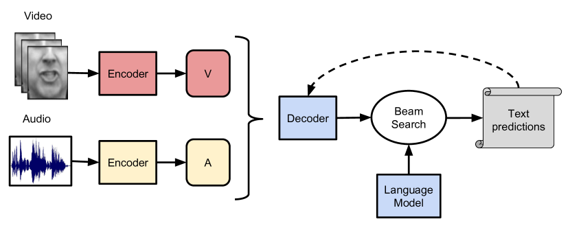
Figure 1: Outline of the audio-visual speech recognition pipeline.

2 Background

2.1 CTC vs sequence-to-sequence architectures

For the most part, end-to-end deep learning approaches for sequence prediction can be divided into two types.

The first type uses a neural network as an emission model which outputs the likelihood of each output symbol (e.g. phonemes) given the input sequence (e.g. audio). These methods generally employ a second phase of decoding using a Hidden Markov Model [25]. One such version of this variant is the Connectionist Temporal Classification (CTC) [22], where the model predicts frame-wise labels and then looks for the optimal alignment between the frame-wise predictions and the output sequence. The main weakness of CTC is that the output labels are not conditioned on each other (it assumes each unit is independent), and hence a language model is employed as a post-processing step. Note that some alternatives to jointly train the two step process has been proposed [21]. Another limitation of this approach is that it assumes a monotonic ordering between input and output sequences. This assumption is suitable for ASR and transcription for example, but not for machine translation.

The second type is sequence-to-sequence models [46, 9] (seq2seq) that first read all of the input sequence before predicting the output sentence. A number of papers have adopted this approach for speech recognition [11, 10]: for example, Chan et al. [7] proposes an elegant sequence-to-sequence method to transcribe audio signal to characters. Sequence-to-sequence decodes an output symbol at time $t$ (e.g. character or word) conditioned on previous outputs $1,\ldots,t-1$. Thus, unlike CTC-based models, the model implicitly learns a language model over output symbols, and no further processing is required. However, it has been shown [7, 26] that it is beneficial to incorporate an external language model in the decoding of sequence-to-sequence models as well. This way it is possible to leverage larger text-only corpora that contain much richer natural language information than the limited aligned data used for training the acoustic model.

Regarding architectures, while CTC-based or seq2seq approaches traditionally relied on recurrent networks, recently there has been a shift towards purely convolutional models [6]. For example, fully convolutional networks have been used for ASR with CTC [51, 55] or a simplified variant [16, 32, 54].

2.2 Related works

Lip reading. There is a large body of work on lip reading using non deep learning methods. These methods are thoroughly reviewed in [56], and we will not repeat this here. A number of papers have used Convolutional Neural Networks (CNNs) to predict phonemes [37] or visemes [29] from still images, as opposed to recognising to full words or sentences. A phoneme is the smallest distinguishable unit of sound that collectively make up a spoken word; a viseme is its visual equivalent.

For recognising full words, Petridis et al. [39] train an LSTM classifier on a discrete cosine transform (DCT) and deep bottleneck features (DBF). Similarly, Wand et al. [50] use an LSTM with HOG input features to recognise short phrases. The shortage of training data in lip reading presumably contributes to the continued use of hand crafted features. Existing datasets consist of videos with only a small number of subjects, and also a limited vocabulary ($<$60 words), which is also an obstacle to progress. Chung and Zisserman [13] tackles the small-lexicon problem by using faces in television broadcasts to assemble the LRW dataset with a vocabulary size of 500 words. However, as with any word-level classification task, the setting is still distant from the real-world, given that the word boundaries must be known beforehand. Assael et al. [4] uses a CNN and LSTM-based network and (CTC) [22] to compute the labelling. This reports strong speaker-independent performance on the constrained grammar and 51 word vocabulary of the GRID dataset [17].

A deeper architecture than LipNet [4] is used by [45], who propose a residual network with 3D convolutions to extract more powerful representations. The network is trained with a cross-entropy loss to recognise words from the LRW dataset. Here, the standard ResNet architecture [24] is modified to process 3D image sequences by changing the first convolutional and pooling blocks from 2D to 3D.

In our earlier work [12], we proposed a WLAS sequence-to-sequence model based on the LAS ASR model of [7] (the acronym WLAS are for Watch, Listen, Attend and Spell, and LAS for Listen, Attend and Spell). The WLAS model had a dual attention mechanism – one for the visual (lip) stream, and the other for the audio (speech) stream. It transcribed spoken sentences to characters, and could handle an input of vision only, audio only, or both.

In independent and concurrent work, Shillingford et al. [43], design a lip reading pipeline that uses a network which outputs phoneme probabilities and is trained with CTC loss. At inference time, they use a decoder based on finite state transducers to convert the phoneme distributions into word sequences. The network is trained on a very large scale lip reading dataset constructed from YouTube videos and achieves a remarkable 40.9% word error rate.

Audio-visual speech recognition. The problems of audio-visual speech recognition (AVSR) and lip reading are closely linked. Mroueh et al. [36] employs feed-forward Deep Neural Networks (DNNs) to perform phoneme classification using a large non-public audio-visual dataset. The use of HMMs together with hand-crafted or pre-trained visual features have proved popular – [48] encodes input images using DBF; [20] used DCT; and [38] uses a CNN pre-trained to classify phonemes; all three combine these features with HMMs to classify spoken digits or isolated words. As with lip reading, there has been little attempt to develop AVSR systems that generalise to real-world settings.

Petridis et al. [40] use an extended version of the architecture of [45] to learn representations from raw pixels and waveforms which they then concatenate and feed to a bidirectional recurrent network that jointly models the audio and video sequences and outputs word labels.

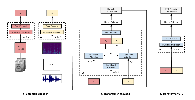
Figure 2: Audio-visual speech recognition models. (a) Common encoder: The visual image sequence is processed by a spatio-temporal ResNet, while the audio features are the spectrograms obtained by applying Short Time Fourier Transform (STFT) to the audio signal. Each modality is then encoded by a separate Transformer encoder. (b) TM-seq2seq: a Transformer model. On every decoder layer, the video (V) and audio (A) encodings are attended to separately by independent multi-head attention modules. The context vectors produced for the two modalities, $V_{c}$ and $A_{c}$ respectively, are concatenated channel-wise and fed to the feed forward layers. K, V and Q denote the Key, Value and Query tensors for the multi-head attention blocks. For the self-attention layers it is always $Q=K=V$, while for the encoder-decoder attentions, $K$ = $V$ are the encodings (V or A), while $Q$ is the previous layer’s output (or, for the first layer, the prediction of the network at the previous decoding step). (c) TM-CTC: Transformer CTC, a model composed of stacks of self-attention and feed forward layers, producing CTC posterior probabilities for every input frame. For full details on the multi-head attention and feed forward blocks refer to Appendix B.

3 Architectures

In this section, we describe model architectures for audio-visual speech recognition, for which we explore two variants, based on the recently proposed Transformer model [49]: i) an encoder-decoder attention structure for training in a seq2seq manner and ii) a stack of self-attention blocks for training with CTC loss. The architecture is outlined in Figure 2. The general model receives two input streams, one for video (V) and one for audio (A).

3.1 Audio Features

For the acoustic representation we use 321-dimensional spectral magnitudes, computed with a 40ms window and 10ms hop-length, at a 16 kHz sample rate. Since the video is sampled at $25$ fps ($40$ ms per frame), every video input frame corresponds to $4$ acoustic feature frames. We concatenate the audio features in groups of $4$, in order to reduce the input sequence length as is common for stable CTC training [42, 8], while at the same time achieving a common temporal-scale for both modalities.

3.2 Vision Module (VM)

The input images are 224$\times$224 pixels, sampled at 25 fps and contain the speaker’s face. We crop a 112$\times$112 patch covering the region around the mouth, as shown in Figure 3. To extract visual features representing the lip movement, we use a spatio-temporal visual front-end that is based on [45]. The network applies 3D convolutions on the input image sequence, with a filter width of $5$ frames, followed by a 2D ResNet that gradually decreases the spatial dimensions with depth. The layers are listed in full detail in Appendix A. For an input sequence of $T\times H\times W$ frames, the output is a $T\times\frac{H}{32}\times\frac{W}{32}\times 512$ tensor (i.e. the temporal resolution is preserved) that is then average-pooled over the spatial dimensions, yielding a $512$-dimensional feature vector for every input video frame.

3.3 Common self-attention Encoder

Both variants that we consider use the same self-attention-based encoder architecture. The encoder is a stack of multi-head self-attention layers, where the input tensor serves as the query, key and value for the attention at the same time. A separate encoder is used for each modality as shown in Figure 2 (a). The information about the sequence order of the inputs is fed to the model via fixed positional embeddings in the form of sinusoid functions.

3.4 Sequence-to-sequence Transformer (TM-seq2seq)

In this variant, separate attention heads are used for attending on the video and audio embeddings. In every decoder layer, the resulting video and audio contexts are concatenated over the channel dimension and propagated to the feedforward block. The attention mechanisms for both modalities receive as queries the output of the previous decoding layer (or the decoder input in the case of the first layer). The decoder produces character probabilities which are directly matched to the ground truth labels and trained with a cross-entropy loss. More details about the multi-head attention and feed-forward building blocks are given in Appendix B.

3.5 CTC Transformer (TM-CTC)

The TM-CTC model concatenates the video and audio encodings and propagates the result through a stack of self-attention / feedforward blocks, same as the one used in the encoders. The outputs of the network are the CTC posterior probabilities for every input frame and the whole stack is trained with CTC loss.

3.6 External Language Model (LM)

For decoding both variants, during inference, we use a character-level language model. It is a recurrent network with 4 unidirectional layers of 1024 LSTM cells each. The language model is trained to predict one character at a time, receiving only the previous character as input. Decoding for both models is performed with a left-to-right beam search where the LM log-probabilities are combined with the model’s outputs via shallow fusion [26]. More details on decoding are given in Appendices C and D.

3.7 Single modality models

The audio-visual models described in this section can be used when only one of the two modalities is present. Instead of concatenating the attention vectors for TM-seq2seq or the encodings for TM-CTC, only the vector from the available modality is used.

4 Dataset

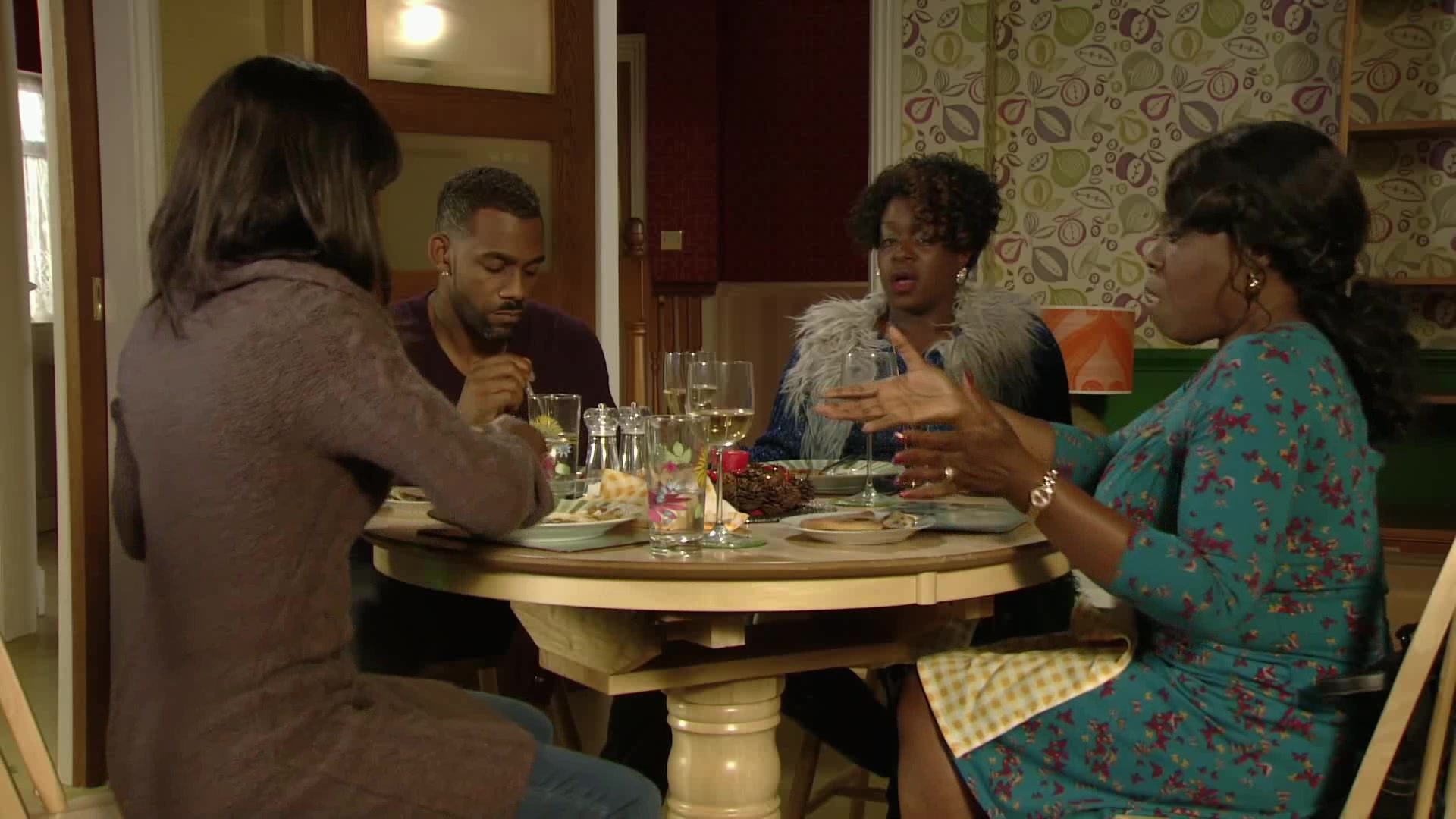
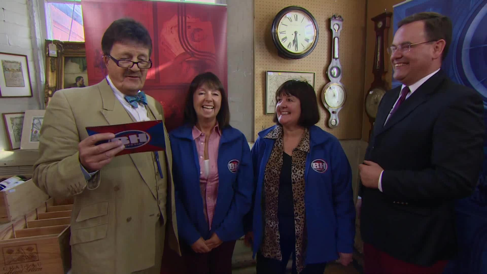
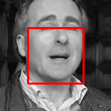
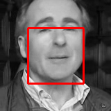
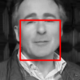
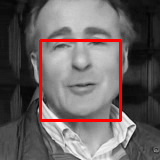
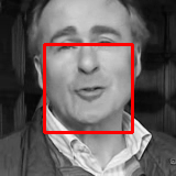
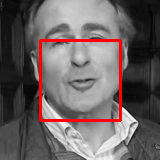
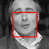
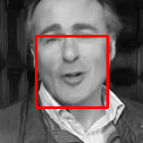
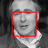
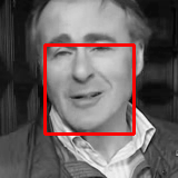
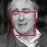
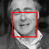
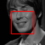
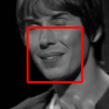
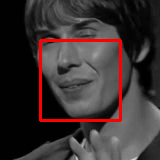
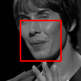
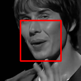
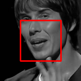
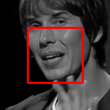
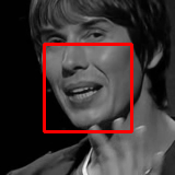
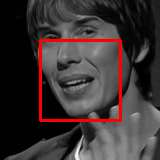
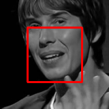
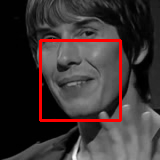
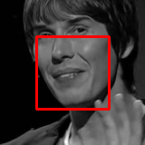
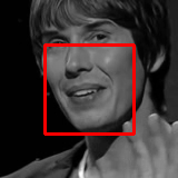
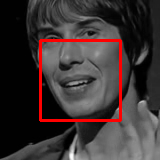
Figure 3: Top: Original still images from videos used in the making of the LRS2-BBC dataset. Bottom: The mouth motions from two different speakers. The network sees the areas inside the red squares.

In this section, we describe the multi-stage pipeline for automatically generating a large-scale dataset, LRS2-BBC, for audio-visual speech recognition. Using this pipeline, we have been able to collect thousands of hours of spoken sentences and phrases along with the corresponding facetrack. We use a variety of BBC programs from Dragon’s Den to Top Gear and Countryfile.

The processing pipeline is summarised in Figure 4. Most of the steps are based on the methods described in [13] and [14], but we give a brief sketch of the method here.

Figure 4: Pipeline to generate the dataset.

Video preparation. A CNN face detector based on the Single Shot MultiBox Detector (SSD) [33] is used to detect face appearances in the individual frames. Unlike the HOG-based detector [27] used by previous works, the SSD detects faces from all angles, and shows a more robust performance whilst being faster to run.

The shot boundaries are determined by comparing color histograms across consecutive frames [31]. Within each shot, face tracks are generated from face detections based on their positions, as feature-based trackers such as KLT [34] often fail when there are extreme changes in viewpoints.

Audio and text preparation. The subtitles in television are not broadcast in sync with the audio. The Penn Phonetics Lab Forced Aligner [53] is used to force-align the subtitle to the audio signal. Errors exist in the alignment as the transcript is not verbatim – therefore the aligned labels are filtered by checking against the commercial IBM Watson Speech to Text service.

AV sync and speaker detection. In broadcast videos, the audio and the video streams can be out of sync by up to around one second, which can cause problems when the facetrack corresponding to a sentence is being extracted. A multi-view adaptation [15] of the two-stream network described in [14] is used to synchronise the two streams. The same network is also used to determine which face’s lip movements match the audio, and if none matches, the clip is rejected as being a voice-over.

Sentence extraction. The videos are divided into individual sentences/ phrases using the punctuations in the transcript. The sentences are separated by full stops, commas and question marks; and are clipped to 100 characters or 10 seconds, due to GPU memory constraints. We do not impose any restrictions on the vocabulary size.

The LRS2-BBC dataset is divided into development (train/val) and test sets according to broadcast date. The dataset also has a “pre-train” set that contains sentence excerpts which may be shorter or longer than the full sentences included in the development set, and are annotated with the alignment boundaries of every word. The statistics of these sets are given in Table I. The table also compares the ‘Lip Reading Sentences’ (LRS) series of datasets to the largest existing public datasets. In addition to LRS2-BBC, we use MV-LRS and LRS3-TED for training and evaluation.

Dataset	Source	Split	Dates	# Spk.	# Utt.	Word inst.	Vocab	# hours
GRID [17]	-	-	-	51	33,000	165k	51	27.5
MODALITY [18]	-	-	-	35	5,880	8,085	182	31
LRW [13]	BBC	Train-val	01/2010 - 12/2015	-	514k	514k	500	165
		Test	01/2016 - 09/2016	-	25k	25k	500	8
LRS [12] ${\dagger}$	BBC	Train-val	01/2010 - 02/2016	-	106k	705k	17k	68
		Test	03/2016 - 09/2016	-	12k	77k	6,882	7.5
MV-LRS [15] ${\dagger}$	BBC	Pre-train	01/2010 - 12/2015	-	430k	5M	30k	730
		Train-val	01/2010 - 12/2015	-	70k	470k	15k	44.4
		Test	01/2016 - 09/2016	-	4,305	30k	4,311	2.8
LRS2-BBC	BBC	Pre-train	01/2010 - 02/2016	-	96k	2M	41k	195
		Train-val	01/2010 - 02/2016	-	47k	337k	18k	29
		Test	03/2016 - 09/2016	-	1,243	6,663	1,693	0.5
		Text-only	01/2016 - 02/2016	-	8M	26M	60k	-
LRS3-TED [3]	TED & TEDx (YouTube)	Pre-train	-	5,075	132k	4.2M	52k	444
		Train-val	-	3,752	32k	358k	17k	30
		Test	-	452	1,452	11k	2,136	1
		Text-only	-	5,075	1.2M	7.2M	57k	-

TABLE I: Statistics on the Lip Reading Sentences (LRS) audio-visual datasets, and other existing large-scale lip reading datasets. Division of training, validation and test data; and the number of utterances, number of word instances and vocabulary size of each partition. Utt: Utterances. ${\dagger}$: Not available to the public due to license restrictions.

Datasets for training external language models. To train the language models used for evaluation on each audio-visual dataset, we use a text corpus containing the full subtitles of the videos from which the dataset’s training set was generated. The text-only corpus contains $26M$ words.

5 Training strategy

In this section, we describe the strategy used to effectively train the models, making best use of the limited amount of data available. The training proceeds in four stages: i) the visual front-end module is trained; ii) visual features are generated for all the training data using the vision module; iii) the sequence processing module is trained on the frozen visual features; iv) the whole network is trained end-to-end.

5.1 Pre-training visual features

We pre-train the visual front-end on word excerpts from the MV-LRS [15] dataset, using a 2-layer temporal convolution back-end to classify every clip with a word label similarly to [45]. We perform data augmentation in the form of horizontal flipping, removal of random frames [4, 45], and random shifts of up to $\pm 5$ pixels in the spatial dimensions and of $\pm 2$ frames in the temporal dimension.

5.2 Curriculum learning

Sequence to sequence learning has been reported to converge very slowly when the number of timesteps is large, because the decoder initially has a hard time extracting the relevant information from all the input steps [7]. Even though our models do not contain any recurrent modules, we found it beneficial to follow a curriculum instead of immediately training on full sentences.

We introduce a new strategy where we start training only on single word examples, and then let the sequence length grow as the network trains. These short sequences are parts of the longer sentences in the dataset. We observe that the rate of convergence on the training set is several times faster, while the curriculum also significantly reduces overfitting, presumably because it works as a natural way of augmenting the data.

The networks are first trained on the frozen features of the pre-train sets from MV-LRS, LRS2-BBC and LRS3-TED. We deal with the difference in utterance lengths by zero-padding the sequences to a maximum length, which we gradually increase. We then separately fine-tune end-to-end on the train-val set of LRS2-BBC or LRS3-TED, according to which set we are evaluating on.

5.3 Training with noisy audio & multi-modal training

The audio-only models are initially trained with clean input audio. Networks with multi-modal inputs can often be dominated by one of the modes [19]. In our case we observe that for the audio-visual models the audio signal dominates, because speech recognition is a significantly easier problem than lip reading. To help prevent this from happening, we add babble noise with 0dB SNR to the audio stream with probability $p_{n}=0.25$ during training.

To assess and improve tolerance to audio noise, we then fine-tune the audio-only and audio-visual models in a setting where babble noise with 0dB SNR is always added to the original audio. We synthesize the babble noise samples by mixing the signals of 20 different audio samples from the LRS2-BBC dataset.

5.4 Implementation details

The output size of the network is 40, accounting for the 26 characters in the alphabet, the 10 digits, and tokens for [space] and [pad]. For TM-seq2seq we use an extra [sos] token and for TM-CTC the [blank] token. We do not model punctuation, as the transcriptions of the datasets do not contain any.

The TM-seq2seq is trained using teacher forcing – we supply the ground truth of the previous decoding step as the input to the decoder, while during inference we feed back the decoder prediction.

Our implementation is based on the TensorFlow library [1] and trained on a single GeForce GTX 1080 Ti GPU with 11GB memory. The network is trained using the ADAM optimiser [28] with the default parameters and an initial learning rate of $10^{-4}$, which is reduced by a factor of 2 every time the validation error plateaus, down to a final learning rate of $10^{-6}$. For all the models we use dropout with $p=0.1$ and label smoothing.

6 Experiments

In this section we evaluate and compare the proposed architectures and training strategies. We also compare our methods to the previous state of the art.

We train as described in section 5.2 and evaluate the fine-tuned models for LRS2-BBC and LRS3-TED on the independent test set of the respective dataset. The inference and evaluation procedures are described below.

Test time augmentation. During inference we perform 9 random transforms (horizontal flipping of the video frames and spatial shifts up to $\pm 5$ pixels) on every video sample, and pass the perturbed sequences through the network, in addition to the original. For TM-seq2seq we average the resulting logits whereas for TM-CTC we average the visual features.

Beam search. Decoding is performed with beam search of width 35 for TM-Seq2seq and 100 for TM-CTC (the values were determined on a held-out validation set from the train-val split of LRS2-BBC).

		LRS2-BBC		LRS3-TED
	M		+ extLM		+ extLM
Google S2T${\dagger}$	A	20.9%		10.4%
WAS [12]	V	70.4%	-	-	-
TM-CTC	V	65.0%	54.7%	74.7%	66.3%
TM-CTC	A	15.3%	10.1%	13.8%	8.9%
TM-CTC	AV	13.7%	8.2%	12.3%	7.5%
TM-seq2seq	V	49.8%	48.3%	59.9%	58.9%
TM-seq2seq	A	10.5%	9.7%	9.0%	8.3%
TM-seq2seq	AV	9.4%	8.5%	8.0%	7.2%
Noisy
Google S2T${\dagger}$	A	86.3%		70.3%
TM-CTC	A	64.7%	53.4%	65.6%	56.3%
TM-CTC	AV	33.5%	23.6%	37.2%	27.7%
TM-seq2seq	A	58.0%	57.4%	60.5%	57.9%
TM-seq2seq	AV	35.9%	34.2%	44.3%	42.5%

TABLE II: Word error rates (WER) on the LRS2-BBC and LRS3-TED datasets. The second column (M) specifies the input modalities: V, A, and AV denote video-only, audio-only, and audio-visual models respectively, while + extLM denotes decoding with the external language model. ${\dagger}$ https://cloud.google.com/speech-to-text, accessed 3 July 2018.

Evaluation protocol. For all experiments, we report the Word Error Rate (WER) which is defined as $\mathtt{WER}=(S+D+I)/N$, where $S$, $D$ and $I$ are the number of substitutions, deletions, and insertions respectively to get from the reference to the hypothesis, and $N$ is the number of words in the reference.

Experimental setup. The rest of this section is structured as follows: First we present results on lip reading, where only the video is used as input. We then use the full models for audio-visual speech recognition, where the video and audio are assumed to be properly synchronised. To assess the robustness of our models in noisy environments we also train and test in a setting where babble noise is artificially added to the utterances. Finally we present some experiments on non-synchronised video and audio. The results for all experiments are summarized in Table II, where we report word error rates depending on whether a language model is used during decoding or not.

6.1 Lips only

Results. The best performing network is TM-seq2seq, which achieves a WER of $48.3\%$ on LRS2-BBC when decoded with a language model, an absolute improvement of over $22\%$ compared to the previous $70.4\%$ state-of-the-art [12]. This model also sets a baseline for LRS3-TED at 58.9%.

In Figure 5 we show how the WER changes as a function of the number of words in a test sentence. Figure 6 shows the performance of the models on the 30 most common words. Figure 7 shows the effect of increasing the beam width for the video-only TM-seq2seq model when evaluating on LRS2-BBC. It is noteworthy that increasing the beam width is more beneficial when decoding with the external language model (+ extLM).

Decoding examples. The model learns to correctly predict complex unseen sentences from a wide range of content – examples are shown in Table III.

but this particular reality was not inevitable
it would have been completely alien to the rest of london
comes from one of the most beautiful parts of the world
everyone has gone home happy and that’s what it’s all about
especially when it comes to climate change
but it’s a different type of animal I want to show you right now
but these are one of the most wary birds in the world
there’s always historical treasures to look at
and so how does your brain give you that detail
but this is the source of innovation
the choices don’t make sense because it’s the wrong question
but it’s a global phenomenon
mortality is not going down it’s going up

TABLE III: Examples of unseen sentences that TM-seq2seq correctly predicts (video only).

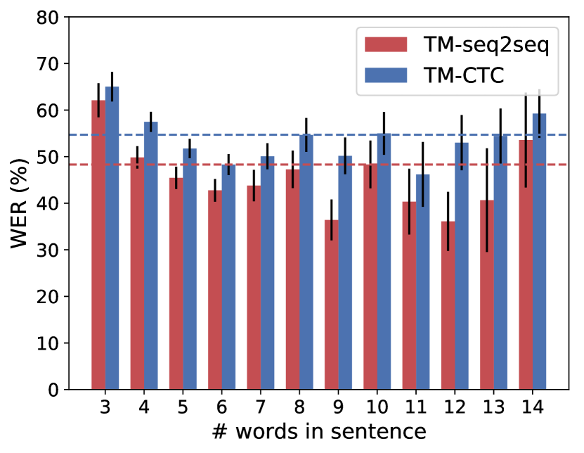
Figure 5: Word error rate per number of words in the sentence for the video-only models, evaluated on the test set of LRS2-BBC. We exclude sentence sizes represented by less than 5 samples in the set (i.e. 15, 16 and 19 words). The dashed lines show the average WER over all the sentences. For both models, the WER is relatively uniform for different sentence sizes. However samples with very few words (3) appear to be more difficult, presumably because they provide less context.

Figure 6: Per word F1, Precision and Recall rates, on the 30 most common words in the LRS2-BBC test set, for the video-only models. The measures are calculated via the minimum edit-distance operations (details in Appendix E). For all words and both models, precision is higher than recall.

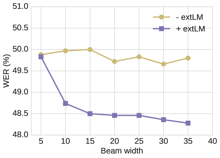
Figure 7: The effect of beam width on Word Error Rate for the video-only TM-seq2seq model, when evaluating on LRS2-BBC.

6.2 Audio-visual speech recognition

The visual information can be used to improve the performance of ASR, particularly in environments with background noise [36, 38, 40]. Here, we analyse the performance of the audio-visual models described in Section 3.

Results. The results in Table II demonstrate that the mouth movements provide important cues in speech recognition when the audio signal is noisy; and give an improvement in performance even when the audio signal is clean – for example the word error rate is reduced from 10.1% for audio only to 8.2%, when using the audio-visual TM-CTC model. The gains when using the audio-visual TM-seq2seq compared to the audio-only model are similar.

Decoding examples. Table IV shows some of the many examples where the model fails to predict the correct sentence from the lips or the audio alone, but successfully deciphers the words when both streams are present.

	Transcription	WER %
GT	your job needs to be challenging
V	job is to be challenging	33
A	your child needs to be challenging	16
AV	your job needs to be challenging	0
GT	I mean I thought poetry was just self expression
V	I mean I thought poetry would just suffer as pressure	44
A	I mean not thought poetry was just self expression	11
AV	I mean I thought poetry was just self expression	0
GT	cluster bombs left behind
V	unless you perhaps have blind	125
A	close to bombs left behind	25
AV	cluster bombs left behind	0
GT	I was the first non family investor in amazon
V	I was the first not family of us are absurd	55
A	I was the first non family in bester and amazon	33
AV	I was the first non family investor in amazon	0

TABLE IV: Examples of AVSR results. GT: Ground Truth; A: Audio only; V: Video only; AV: Audio-visual.

Alignment and attention visualisation. The encoder-decoder attention mechanism of the TM-seq2seq model generates explicit alignment between the input video frames and the hypothesised character output. Figure 9 visualises the alignment of the characters “comes from one of the most beautiful parts of the world” and the corresponding video frames. Since the architecture contains multiple attention heads, we obtain the alignment by averaging the attention masks over all the decoder layers in the log domain.

Noisy audio. We perform the audio-only and audio-visual experiments with noisy audio, synthesized by adding babble noise to the original utterances. Speech recognition in a noisy environment is extremely challenging, as can be seen from the significantly lower performance of the off-the-shelf Google S2T ASR baseline (over 60% performance degradation compared to clean). This difficulty is also reflected on the performance of our audio-only models, that the word error rates similar to the ones obtained when only using the lips. However combining the two modalities provides a significant improvement, with the word error rate dropping significantly, by up to $30\%$. Notably, the audio-visual models perform much better than either the video-only, or audio-only ones under the presence of loud background noise.

AV attention visualization. In Figure 10 we compare the attention masks of different TM-seq2seq models in the presence and absence of additive babble noise in the audio stream.

6.3 Out-of-sync audio and video

Here, we assess the performance of the audio-visual models when the audio and video inputs are not temporally aligned. Since the audio and video have been synchronised in our dataset, we synthetically shift the video frames to achieve an out-of-sync effect. We evaluate the performance on de-synchronised samples of the LRS2-BBC dataset. We consider the TM-CTC and TM-seq2seq architectures, with and without fine-tuning on randomly shifted samples. The results are shown in Figure 8. It is clear that the TM-seq2seq architecture is more resistant to these shifts. We only need to calibrate the model for one epoch for the out-of-sync effect to practically vanish. This showcases the advantage of employing independent encoder-decoder attention mechanisms for the two modalities. In contrast, TM-CTC, that concatenates the two encodings, struggles to deal with the shifts, even after several epochs of fine-tuning.

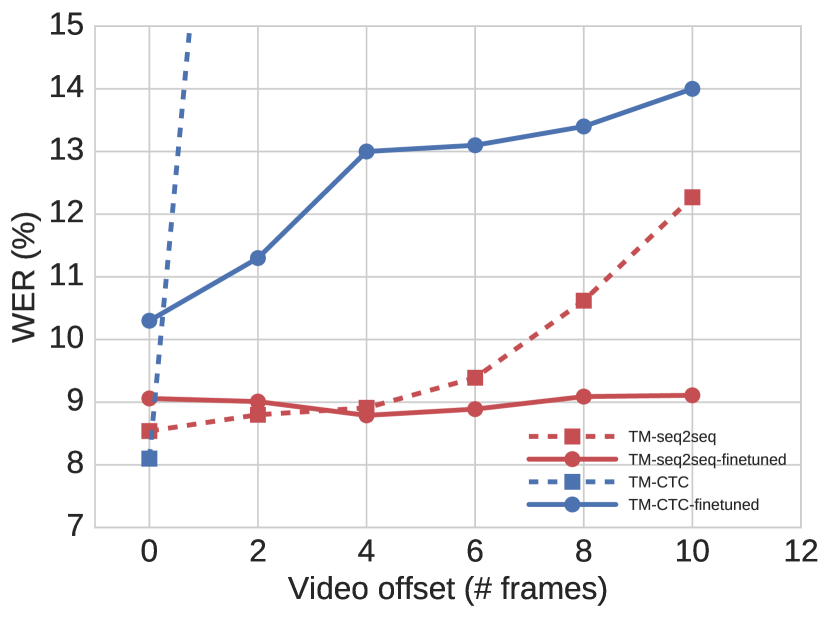
Figure 8: WER scored by the audio-visual models on LRS2-BBC when the video frames are artificially shifted by a number of frames compared to audio. The TM-seq2seq model is only fine-tuned for one epoch, while CTC for 4 epochs on the train-val set.

Figure 9: Alignment between the video frames and the character output with TM-seq2seq. The alignment is produced by averaging all the encoder-decoder attention heads over all the decoder layers in the log domain.

(a) Clean audio spectrogram

(b) Noisy audio spectrogram

(c) A clean

(d) A noisy

(e) V

(f) AV clean - audio attention

(g) AV noisy - audio attention

(h) AV noisy - video attention

Figure 10: Visualization of the effect of additive noise on the attention masks of the different TM-seq2seq models. We show the attentions on (a) the clean audio utterance, and (b) on the noisy utterance which we obtain by adding babble noise to the 25 central audio frames. Comparing (c) with (d), the attention of the audio-only models appears to be more spread around the area where the noise is applied, while the last frames are not attended upon. Similarly for the audio-visual model, the audio attention is more focused when the audio is clean (f) compared to when it is noisy (g). The ground truth transcription of the sentence is “one of the articles there is about the queen elizabeth”. Observing the transcriptions, we see that the audio-only model (d) does not predict the central words correctly when noise is added, however the audio-visual model (g & h) successfully transcribes the sentence, by leveraging the visual cues. Interestingly, in this particular example, the transcription that the video-only model outputs (e) is completely wrong; the combination of both modalities however yields a correct prediction. Finally, the attention mask of the AV model on the video input (f) has a clear monotonic trend and is similar to the one of the video-only model (e); this also verifies that the model indeed learns to use the video modality even when audio is present.

6.4 Discussion on seq2seq vs CTC

The TM-seq2seq model performs significantly better for lip-reading in terms of WER, when no audio is supplied. For audio-only or audio-visual tasks, the two methods perform similarly. However the CTC models appear to handle background noise better; in the presence of loud babble noise, both the audio-only and audio-visual TM-seq2seq models perform significantly worse that their TM-CTC counterparts.

Training time. The TM-seq2seq models have a more complex architecture and are harder to train, with the full audio-visual model taking approximately 8 days to complete the full curriculum for both datasets, on a single GeForce Titan X GPU with 12GB memory. In contrast, the audiovisual TM-CTC model trains faster i.e. in approximately 5 days on the same hardware. It should be noted however that since both architectures contain no recurrent modules and no batch normalization, their implementation can be heavily parallelized into multiple GPUs.

Inference time. Decoding of the TM-CTC model does not require auto-regression and therefore the CTC probabilities need only be evaluated once, regardless of the beam width $W$. This is not the case for TM-seq2seq, where for every step of the beam search, the decoder subnetwork needs to be evaluated $W$ times. This makes the decoding of the CTC model faster, which can be an important factor for deployment.

Language modelling. Both models perform better when an external language model is incorporated in the beam search, however the gains are much higher for TM-CTC, since no explicit language consistency is enforced by the visual model alone.

Generalization to longer sequences. We observed that the TM-CTC model generalizes better and adapts faster as the sequence lengths are increased during the curriculum learning. We believe this also affects the training time as the latter takes more epochs to converge.

7 Conclusion

In this paper, we introduced a large-scale, unconstrained audio-visual dataset, LRS2-BBC, formed by collecting and preprocessing thousands of videos from the British television.

We considered two models that can transcribe audio and video sequences of speech into characters and showed that the same architectures can also be used when only one of the modalities is present. Our best visual-only model surpasses the performance of the previous state-of-the-art on the LRS2-BBC lip reading dataset by a large margin, and sets a strong baseline for the recently released LRS3-TED. We finally demonstrate that visual information helps improve speech recognition performance even when the clean audio signal is available. Especially in the presence of noise in the audio, combining the two modalities leads to a significant improvement.

Appendix A Visual front-end architecture

The details of the spatio-temporal front-end are given in Table V.

Layer Type	Filters	Output dimensions
Conv 3D	$5\times 7\times 7$, $64$, $/[1,2,2]$	$T\times\frac{H}{2}\times\frac{W}{2}\times 64$
Max Pool 3D	$/[1,2,2]$	$T\times\frac{H}{4}\times\frac{W}{4}\times 64$
Residual Conv 2D	[$3\times 3$, $64$] $\times 2$ $/1$	$T\times\frac{H}{4}\times\frac{W}{4}\times 64$
Residual Conv 2D	[$3\times 3$, $64$] $\times 2$ $/1$	$T\times\frac{H}{4}\times\frac{W}{4}\times 64$
Residual Conv 2D	[$3\times 3$, $128$] $\times 2$ $/2$	$T\times\frac{H}{8}\times\frac{W}{8}\times 128$
Residual Conv 2D	[$3\times 3$, $128$] $\times 2$ $/1$	$T\times\frac{H}{8}\times\frac{W}{8}\times 128$
Residual Conv 2D	[$3\times 3$, $256$] $\times 2$ $/2$	$T\times\frac{H}{16}\times\frac{W}{16}\times 256$
Residual Conv 2D	[$3\times 3$, $256$] $\times 2$ $/1$	$T\times\frac{H}{16}\times\frac{W}{16}\times 256$
Residual Conv 2D	[$3\times 3$, $512$] $\times 2$ $/2$	$T\times\frac{H}{32}\times\frac{W}{32}\times 512$
Residual Conv 2D	[$3\times 3$, $512$] $\times 2$ $/1$	$T\times\frac{H}{32}\times\frac{W}{32}\times 512$

TABLE V: Architecture details for the spatio-temporal visual front-end [45]. The strides for the residual 2D convolutional blocks apply to the first layer of the block only (i.e. the total down-sampling factor in the network is 32). A short cut connection is added after every pair of 2D convolutions [24]. The 2D convolutions are applied separately on every time-frame.

Appendix B Transformer architecture details

The details of the building blocks used by our models are outlined in Figure 11. The same multi-head attention block shown is used for both the self-attention and encoder-decoder attention layers of the models. A multi-head attention block, as described by Vaswani et al. [49], receives a query ($Q$), a key ($K$) and a value ($V$) tensor as inputs and produces $h$ context vectors, one for every attention head $i$:

$$Att_{i}(Q,K,V)=softmax(\frac{(W_{i}^{q}Q^{T})^{T}(W_{i}^{k}K^{T})}{\sqrt{d_{k}}})(W_{i}^{v}V^{T})^{T}$$

where $Q$, $K$, and $V$ have size $d_{model}$ and $dk$ = $\frac{d_{model}}{h}$ is the size of every attention head. The $h$ context vectors are concatenated and propagated through a feedforward block that consists of two linear layers with ReLU non-linearities in between. For the self-attention layers it is always $Q=K=V$, while for the encoder-decoder attention of the TM-seq2seq model, $K$ = $V$ are the encoder outputs to be attended upon and $Q$ is the decoder input, i.e. the network’s output at the previous decoding step for the first layer and the output of the previous decoder layer for the rest. We use the same architecture hyperparameters as the original base model of Vaswani et al. [49] with $d_{model}=512$ and $h=8$ attention heads everywhere. The sizes of the two linear layers in the feedforward block are $F1=2048$, $F2=512$.

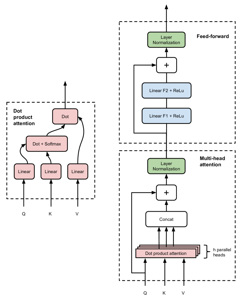
Figure 11: Details of multi-head attention building blocks

Appendix C Seq2Seq decoding with external language model

For decoding with the TM-seq2seq model, we use a left-to right beam search with width $W$ as in [26, 52], with the hypotheses $y$ being scored as follows:

$$score(x,y)=\frac{log\ p(y|x)+\alpha\ log\ p_{LM}(y)}{LP(y)}$$

where $p(y|x)$ and $p_{LM}(y)$ are the probabilities obtained from the visual and language models respectively and LP is a length normalization factor LP(y) = $\Big{(}\frac{5+|y|}{6}\Big{)}^{\beta}$ [52]. We did not experiment with a coverage penalty. The best values for the hyperparameters were determined via grid search on the validation set: for decoding without the external language model they were set to $W=6$, $\alpha=0.0$, $\beta=0.6$ and for decoding with the external language model (+ extLM) to $W=35$, $\alpha=0.1$ $\beta=0.7$.

Appendix D CTC decoding algorithm with external language model

Algorithm 1 describes the CTC decoding procedure with an external language model. It is also a beam search with width W and hyperparameters $\alpha$ and $\beta$ that control the relative weight given to the LM and the length penalty. The beam search is similar to the one described for seq2seq above, with some additional bookkeeping required to handle the emission of repeated and blank characters and normalization LP(y) = $|y|^{\beta}$. We obtain the best results on the validation set with $W=100$, $\alpha=0.5$, $\beta=0.1$.

Algorithm 1 CTC Beam search decoding with Language Model adapted from [35]. Notation: A is the alphabet; $p_{b}(s,t)$ and $p_{nb}(s,t)$ are the probabilities of partial output transcription s resulting from paths ending in blank and non-blank token respectively, given the input sequence up to time $t$; $p(s,t)=p_{b}(s,t)+p_{nb}(s,t)$.

Parameters CTC probabilities $p^{ctc}_{1:T}$, word dictionary, beam width $W$, hyperparameters $\alpha$, $\beta$

initialize $\mathbf{B_{t}}\leftarrow$ {$\varnothing$}; $\mathbf{p_{b}(\varnothing,0)}\leftarrow$ 1; $\mathbf{p_{nb}(\varnothing,0)}\leftarrow$ 0

for $t=1$ to $T$ do

     $\mathbf{B_{t-1}}\leftarrow$ $W$ prefixes with highest $\frac{log\ p(s,t)}{|s|^{\beta}}$ in $\mathbf{B}_{t}$

     $\mathbf{B_{t}}\leftarrow$ {}

     for prefix $s$ in $\mathbf{B_{t-1}}$ do

         $c^{-}\leftarrow$ last character of $s$

         $p_{b}(s,t)\leftarrow p^{ctc}_{t}(-,t)p(s,t-1)$ $\triangleright$ adding a blank

         $p_{nb}(s,t)\leftarrow p^{ctc}_{t}(c^{-},t)p_{nb}(s,t-1)$ $\triangleright$ repeated

         add $s$ to $\mathbf{B_{t}}$

         for character $c$ in $A$ do

              $s^{+}\leftarrow s+c$

              if $s$ does not end in $c$ then

                  $p_{c}\leftarrow p^{ctc}_{t}(c,t)p(s,t-1)p_{LM}(c|s)^{\alpha}$

              else

                  $\triangleright$ repeated chars must have blanks in between

                  $p_{c}\leftarrow p^{ctc}_{t}(c,t)p_{b}(s,t-1)p_{LM}(c|s)^{\alpha}$

              end if

              if $s^{+}$ is already in $\mathbf{B_{t}}$  then

                  $p_{nb}(s^{+},t)\leftarrow p_{nb}(s^{+},t)+p_{c}$

              else

                  add $s^{+}$ to $\mathbf{B_{t}}$

                  $p_{nb}(s,t)\leftarrow 0$

                  $p_{nb}(s^{+},t)\leftarrow p_{c}$

              end if

         end for

     end for

end for

return $max_{s\in B_{t}}\frac{log\ p(s,T)}{|s|^{\beta}}$ in $\mathbf{B}_{T}$

Appendix E Precision and Recall from edit distance

The F1, precision and recall rates shown in figure E, are calculated from the word-wise minimum edit distance operations. For every sample in the evaluation set we can calculate the fewest word substitution, insertion and deletion operations needed to get from the ground truth to the predicted transcription. After aggregating those operations over the evaluation set for every word, we calculate the average measures per word as follows:

$$TP(w)=n_{m}(w)$$

$$FN(w)=\sum_{j}n_{s}(j,w)+n_{i}(w)$$

$$FP(w)=\sum_{j}n_{s}(w,j)+n_{d}(w)$$

$$Precision(w)=\frac{TP(w)}{TP(w)+FP(w)}$$

$$Recall(w)=\frac{TP(w)}{TP(w)+FN(w)}$$

$$F1(w)=2\frac{Precision(w)Recall(w)}{Precision(w)+Recall(w)}$$

where $n_{s}$(w,j) is the total count over the evaluation set of substitutions of word $j$ with word $w$, and $n_{m}$(w), $n_{i}$(w) and $n_{d}$(w) are the total matches, deletions and insertions respectively of word $w$.

References

- [1] M. Abadi, A. Agarwal, P. Barham, E. Brevdo, Z. Chen, C. Citro, G. S. Corrado, A. Davis, J. Dean, M. Devin, et al. Tensorflow: Large-scale machine learning on heterogeneous distributed systems. arXiv preprint arXiv:1603.04467, 2016.
- [2] T. Afouras, J. S. Chung, and A. Zisserman. Deep lip reading: A comparison of models and an online application. In INTERSPEECH, 2018.
- [3] T. Afouras, J. S. Chung, and A. Zisserman. LRS3-TED: a large-scale dataset for visual speech recognition. arXiv preprint arXiv:1809.00496, 2018.
- [4] Y. M. Assael, B. Shillingford, S. Whiteson, and N. de Freitas. Lipnet: Sentence-level lipreading. arXiv:1611.01599, 2016.
- [5] D. Bahdanau, K. Cho, and Y. Bengio. Neural machine translation by jointly learning to align and translate. Proceedings of the International Conference on Learning Representations, 2015.
- [6] S. Bai, J. Z. Kolter, and V. Koltun. An empirical evaluation of generic convolutional and recurrent networks for sequence modeling. arXiv preprint arXiv:1803.01271, 2018.
- [7] W. Chan, N. Jaitly, Q. V. Le, and O. Vinyals. Listen, attend and spell. arXiv preprint arXiv:1508.01211, 2015.
- [8] C. Chiu, T. N. Sainath, Y. Wu, R. Prabhavalkar, P. Nguyen, Z. Chen, A. Kannan, R. J. Weiss, K. Rao, K. Gonina, N. Jaitly, B. Li, J. Chorowski, and M. Bacchiani. State-of-the-art speech recognition with sequence-to-sequence models. CoRR, abs/1712.01769, 2017.
- [9] K. Cho, B. Van Merriënboer, C. Gulcehre, D. Bahdanau, F. Bougares, H. Schwenk, and Y. Bengio. Learning phrase representations using rnn encoder-decoder for statistical machine translation. In EMNLP, 2014.
- [10] J. Chorowski, D. Bahdanau, K. Cho, and Y. Bengio. End-to-end continuous speech recognition using attention-based recurrent NN: first results. In NIPS 2014 Workshop on Deep Learning, 2014.
- [11] J. K. Chorowski, D. Bahdanau, D. Serdyuk, K. Cho, and Y. Bengio. Attention-based models for speech recognition. In Advances in Neural Information Processing Systems, pages 577–585, 2015.
- [12] J. S. Chung, A. Senior, O. Vinyals, and A. Zisserman. Lip reading sentences in the wild. In Proceedings of the IEEE Conference on Computer Vision and Pattern Recognition, 2017.
- [13] J. S. Chung and A. Zisserman. Lip reading in the wild. In Proceedings of the Asian Conference on Computer Vision, 2016.
- [14] J. S. Chung and A. Zisserman. Out of time: automated lip sync in the wild. In Workshop on Multi-view Lip-reading, ACCV, 2016.
- [15] J. S. Chung and A. Zisserman. Lip reading in profile. In Proceedings of the British Machine Vision Conference, 2017.
- [16] R. Collobert, C. Puhrsch, and G. Synnaeve. Wav2letter: An end-to-end convnet-based speech recognition system. CoRR, abs/1609.03193, 2016.
- [17] M. Cooke, J. Barker, S. Cunningham, and X. Shao. An audio-visual corpus for speech perception and automatic speech recognition. The Journal of the Acoustical Society of America, 120(5):2421–2424, 2006.
- [18] A. Czyzewski, B. Kostek, P. Bratoszewski, J. Kotus, and M. Szykulski. An audio-visual corpus for multimodal automatic speech recognition. Journal of Intelligent Information Systems, pages 1–26, 2017.
- [19] C. Feichtenhofer, A. Pinz, and A. Zisserman. Convolutional two-stream network fusion for video action recognition. In Proceedings of the IEEE Conference on Computer Vision and Pattern Recognition, 2016.
- [20] G. Galatas, G. Potamianos, and F. Makedon. Audio-visual speech recognition incorporating facial depth information captured by the kinect. In Signal Processing Conference (EUSIPCO), 2012 Proceedings of the 20th European, pages 2714–2717. IEEE, 2012.
- [21] A. Graves. Sequence transduction with recurrent neural networks. arXiv preprint arXiv:1211.3711, 2012.
- [22] A. Graves, S. Fernández, F. Gomez, and J. Schmidhuber. Connectionist temporal classification: Labelling unsegmented sequence data with recurrent neural networks. In Proceedings of the International Conference on Machine Learning, pages 369–376. ACM, 2006.
- [23] A. Graves and N. Jaitly. Towards end-to-end speech recognition with recurrent neural networks. In Proceedings of the International Conference on Machine Learning, pages 1764–1772, 2014.
- [24] K. He, X. Zhang, S. Ren, and J. Sun. Deep residual learning for image recognition. arXiv preprint arXiv:1512.03385, 2015.
- [25] G. Hinton, L. Deng, D. Yu, G. Dahl, A.-R. Mohamed, N. Jaitly, A. Senior, V. Vanhoucke, P. Nguyen, B. Kingsbury, and T. Sainath. Deep neural networks for acoustic modeling in speech recognition. IEEE Signal Processing Magazine, 29:82–97, November 2012.
- [26] A. Kannan, Y. Wu, P. Nguyen, T. N. Sainath, Z. Chen, and R. Prabhavalkar. An analysis of incorporating an external language model into a sequence-to-sequence model. arXiv preprint arXiv:1712.01996, 2017.
- [27] D. E. King. Dlib-ml: A machine learning toolkit. The Journal of Machine Learning Research, 10:1755–1758, 2009.
- [28] D. P. Kingma and J. Ba. ADAM: A method for stochastic optimization. In Proceedings of the International Conference on Learning Representations, 2015.
- [29] O. Koller, H. Ney, and R. Bowden. Deep learning of mouth shapes for sign language. In Proceedings of the IEEE Conference on Computer Vision and Pattern Recognition, pages 85–91, 2015.
- [30] A. Krizhevsky, I. Sutskever, and G. E. Hinton. ImageNet classification with deep convolutional neural networks. In Advances in Neural Information Processing Systems, pages 1106–1114, 2012.
- [31] R. Lienhart. Reliable transition detection in videos: A survey and practitioner’s guide. International Journal of Image and Graphics, August 2001.
- [32] V. Liptchinsky, G. Synnaeve, and R. Collobert. Letter-based speech recognition with gated convnets. CoRR, abs/1712.09444, 2017.
- [33] W. Liu, D. Anguelov, D. Erhan, C. Szegedy, S. Reed, C.-Y. Fu, and A. C. Berg. SSD: Single shot multibox detector. In Proceedings of the European Conference on Computer Vision, pages 21–37. Springer, 2016.
- [34] B. D. Lucas and T. Kanade. An iterative image registration technique with an application to stereo vision. In Proc. of the 7th International Joint Conference on Artificial Intelligence, pages 674–679, 1981.
- [35] A. L. Maas, Z. Xie, D. Jurafsky, and A. Y. Ng. Lexicon-free conversational speech recognition with neural networks. In Proceedings the North American Chapter of the Association for Computational Linguistics (NAACL), 2015.
- [36] Y. Mroueh, E. Marcheret, and V. Goel. Deep multimodal learning for audio-visual speech recognition. In 2015 IEEE International Conference on Acoustics, Speech and Signal Processing (ICASSP), pages 2130–2134. IEEE, 2015.
- [37] K. Noda, Y. Yamaguchi, K. Nakadai, H. G. Okuno, and T. Ogata. Lipreading using convolutional neural network. In INTERSPEECH, pages 1149–1153, 2014.
- [38] K. Noda, Y. Yamaguchi, K. Nakadai, H. G. Okuno, and T. Ogata. Audio-visual speech recognition using deep learning. Applied Intelligence, 42(4):722–737, 2015.
- [39] S. Petridis and M. Pantic. Deep complementary bottleneck features for visual speech recognition. ICASSP, pages 2304–2308, 2016.
- [40] S. Petridis, T. Stafylakis, P. Ma, F. Cai, G. Tzimiropoulos, and M. Pantic. End-to-end audiovisual speech recognition. CoRR, abs/1802.06424, 2018.
- [41] O. Russakovsky, J. Deng, H. Su, J. Krause, S. Satheesh, S. Ma, S. Huang, A. Karpathy, A. Khosla, M. Bernstein, A. Berg, and F. Li. Imagenet large scale visual recognition challenge. International Journal of Computer Vision, 2015.
- [42] H. Sak, A. W. Senior, K. Rao, and F. Beaufays. Fast and accurate recurrent neural network acoustic models for speech recognition. In INTERSPEECH, 2015.
- [43] B. Shillingford, Y. Assael, M. W. Hoffman, T. Paine, C. Hughes, U. Prabhu, H. Liao, H. Sak, K. Rao, L. Bennett, M. Mulville, B. Coppin, B. Laurie, A. Senior, and N. de Freitas. Large-Scale Visual Speech Recognition. arXiv preprint arXiv:1807.05162, 2018.
- [44] K. Simonyan and A. Zisserman. Very deep convolutional networks for large-scale image recognition. In International Conference on Learning Representations, 2015.
- [45] T. Stafylakis and G. Tzimiropoulos. Combining residual networks with LSTMs for lipreading. In Interspeech, 2017.
- [46] I. Sutskever, O. Vinyals, and Q. Le. Sequence to sequence learning with neural networks. In Advances in neural information processing systems, pages 3104–3112, 2014.
- [47] C. Szegedy, W. Liu, Y. Jia, P. Sermanet, S. Reed, D. Anguelov, D. Erhan, V. Vanhoucke, and A. Rabinovich. Going deeper with convolutions. In Proceedings of the IEEE Conference on Computer Vision and Pattern Recognition, 2015.
- [48] S. Tamura, H. Ninomiya, N. Kitaoka, S. Osuga, Y. Iribe, K. Takeda, and S. Hayamizu. Audio-visual speech recognition using deep bottleneck features and high-performance lipreading. In 2015 Asia-Pacific Signal and Information Processing Association Annual Summit and Conference (APSIPA), pages 575–582. IEEE, 2015.
- [49] A. Vaswani, N. Shazeer, N. Parmar, J. Uszkoreit, L. Jones, A. N. Gomez, L. Kaiser, and I. Polosukhin. Attention Is All You Need. In Advances in Neural Information Processing Systems, 2017.
- [50] M. Wand, J. Koutn, and J. Schmidhuber. Lipreading with long short-term memory. In 2016 IEEE International Conference on Acoustics, Speech and Signal Processing (ICASSP), pages 6115–6119. IEEE, 2016.
- [51] Y. Wang, X. Deng, S. Pu, and Z. Huang. Residual Convolutional CTC Networks for Automatic Speech Recognition. arXiv preprint arXiv:1702.07793, 2017.
- [52] Y. Wu, M. Schuster, Z. Chen, Q. V. Le, M. Norouzi, W. Macherey, M. Krikun, Y. Cao, Q. Gao, K. Macherey, J. Klingner, A. Shah, M. Johnson, X. Liu, L. Kaiser, S. Gouws, Y. Kato, T. Kudo, H. Kazawa, K. Stevens, G. Kurian, N. Patil, W. Wang, C. Young, J. Smith, J. Riesa, A. Rudnick, O. Vinyals, G. Corrado, M. Hughes, and J. Dean. Google’s neural machine translation system: Bridging the gap between human and machine translation. CoRR, abs/1609.08144, 2016.
- [53] J. Yuan and M. Liberman. Speaker identification on the scotus corpus. Journal of the Acoustical Society of America, 123(5):3878, 2008.
- [54] N. Zeghidour, N. Usunier, I. Kokkinos, T. Schatz, G. Synnaeve, and E. Dupoux. Learning filterbanks from raw speech for phone recognition. CoRR, abs/1711.01161, 2017.
- [55] Y. Zhang, M. Pezeshki, P. Brakel, S. Zhang, C. Laurent, Y. Bengio, and A. C. Courville. Towards end-to-end speech recognition with deep convolutional neural networks. CoRR, abs/1701.02720, 2017.
- [56] Z. Zhou, G. Zhao, X. Hong, and M. Pietikäinen. A review of recent advances in visual speech decoding. Image and vision computing, 32(9):590–605, 2014.