Abstract

GAIL is a recent successful imitation learning architecture that exploits the adversarial training procedure introduced in GANs. Albeit successful at generating behaviours similar to those demonstrated to the agent, GAIL suffers from a high sample complexity in the number of interactions it has to carry out in the environment in order to achieve satisfactory performance. We dramatically shrink the amount of interactions with the environment necessary to learn well-behaved imitation policies, by up to several orders of magnitude. Our framework, operating in the model-free regime, exhibits a significant increase in sample-efficiency over previous methods by simultaneously a) learning a self-tuned adversarially-trained surrogate reward and b) leveraging an off-policy actor-critic architecture. We show that our approach is simple to implement and that the learned agents remain remarkably stable, as shown in our experiments that span a variety of continuous control tasks. Video visualisations available at: https://youtu.be/-nCsqUJnRKU.

1 Introduction

Reinforcement learning (RL) is a powerful and extensive framework enabling a learner to tackle complex continuous control tasks (Sutton and Barto,, 1998). Leveraging strong function approximators such as multi-layer neural networks, deep reinforcement learning alleviates the customary preliminary workload consisting in hand-crafting relevant features for the learning agent to work on. While being freed from this engineering burden opens up the framework to an even broader range of complex control and planning tasks, RL remains hindered by its reliance on reward design, referred to as reward shaping. Albeit appealing in theory, shaping often requires an intimidating amount of engineering via trial and error to yield natural-looking behaviours and makes the system prone to premature convergence to local minima (Ng et al.,, 1999).

Imitation learning breaks free from the preliminary reward function hand-crafting step as it does not need access to a reinforcement signal. Instead, imitation learning learns to perform a task directly from expert demonstrations. The emerging policies mimic the behaviour displayed by the expert in those demonstrations. Learning from demonstrations (LfD) has enabled significant advances in robotics (Billard et al.,, 2008) and autonomous driving (Pomerleau,, 1989, 1990). Such models were fit from the expert demonstrations alone in a supervised fashion, without gathering new data in simulation. Albeit efficient when data is abundant, they tend to be frail as the agent strays from the expert trajectories. The ensuing compounding of errors causes a covariate shift (Ross and Bagnell,, 2010; Ross et al.,, 2011). This approach, referred to as behavioral cloning, is therefore poorly adapted for imitation. Those limitations stem from the sequential nature of the problem.

The caveats of behavioral cloning have recently been successfully addressed by Ho and Ermon (Ho and Ermon,, 2016) who introduced a model-free imitation learning method called Generative Adversarial Imitation Learning (GAIL). Leveraging Generative Adversarial Networks (GAN) (Goodfellow et al.,, 2014), GAIL alleviates the limitations of the supervised approach by a) learning a reward surrogate that explains the behaviour shown in the demonstrations and b) following an RL procedure in an inner loop, consisting in performing rollouts in a simulated environment with the learned surrogate as reinforcement signal. Several works have built on GAIL to overcome the weaknesses it inherits from GANs, with a particular emphasis on avoiding mode collapse (Li et al.,, 2017; Hausman et al.,, 2017; Kuefler and Kochenderfer,, 2017), causing policies to fail at displaying the diversity of demonstrated behaviours or skills (Goodfellow,, 2017). However, as the authors point out in the original paper ((Ho and Ermon,, 2016), Section 7), GAIL suffers from severe sample inefficiency. It is this limitation of GAIL that we address in this paper. “Sample-efficient” here means that we focus on limiting the number of agent-environment interactions, in contrast with reducing the number of demonstrations needed by the agent. Although learning from fewer demonstrations is not the primary focus of this work, our experiments span a spectrum of demonstration dataset sizes.

Failures of previous works to address the exceeding sample complexity stems from the on-policy nature of the RL procedure they employ. In such methods, every interaction in a given rollout typically is used to compute the Monte Carlo estimate of the state value by summing the rewards accumulated during the current trajectory. The experienced transitions are then discarded. Holding on to past trajectories to carry out more than a single optimization step might appear viable but often results in destructively large policy updates (Schulman et al.,, 2017). Gradients based on those estimates therefore suffer from high variance, which can be reduced by sampling more intensively, hence the deterring sample complexity.

In this work, we introduce a novel method that successfully addresses the impeding sample inefficiency in the number of simulator queries suffered by previous methods. By designing an off-policy learning procedure relying on the use of retained past experiences, we considerably shrink the amount of interactions necessary to learn good imitation policies. Despite involving an adversarial training procedure and an actor-critic method, both notorious for being prone to instabilities and prohibitively difficult to train, our technique demonstrates consistent stability, as shown in the experimental section. Additionally, our reliance on the deterministic policy gradients allows us to exploit further information about the learned reward function, such as its gradient. Previous methods either ignore it by treating the reward signal as a scalar in a model-free fashion or train a forward model to exploit it. Our method achieves the best of both worlds as it can perform a backward pass from the discriminator to the generator (policy) while remaining model-free.

2 Related Work

Imitation learning aims to learn how to perform tasks solely from expert demonstrations. Two approaches are typically adopted to tackle imitation learning problems: a) behavioral cloning (BC) (Pomerleau,, 1989, 1990), which learns a policy via regression on the state-action pairs from the expert trajectories, and b) apprenticeship learning (AL) (Abbeel and Ng,, 2004), which posits the existence of some unknown reward function under which the expert policy is optimal and learns a policy by i) recovering the reward that the expert is assumed to maximise (an approach called inverse reinforcement learning (IRL)) and ii) running an RL procedure with this recovered signal. As a supervised approach, BC is limited to the available demonstrations to learn a regression model, whose predictions worsen dramatically as the agent strays from the demonstrated trajectories. It then becomes increasingly difficult for the model to recover as the errors compound (Ross and Bagnell,, 2010; Ross et al.,, 2011; Bagnell,, 2015). Only the presence of correcting behaviour in the demonstration dataset can allow BC to produce robust policies. AL alleviates this weakness by entangling learning the reward function and learning the mimicking policy, leveraging the return of the latter to adjust the parameters of the former. Models are trained on traces of interaction with the environment rather than on a fixed state pool, leading to greater generalization to states absent from the demonstrations. Albeit preventing errors from compounding, IRL comes with a high computational cost, as both modelling the reward function and solving the ensuing RL problem (per learning iteration) can be resource intensive (Syed et al.,, 2008; Syed and Schapire,, 2008; Ho et al.,, 2016; Levine et al.,, 2011).

In an attempt to overcome the shortcomings of IRL, Ho and Ermon (Ho and Ermon,, 2016) managed to bypass the need for learning the reward function assumed to have been optimised by the expert when collecting the demonstrations. The proposed approach to AL, Generative Adversarial Imitation Learning (GAIL), relies on an essential step consisting in learning a surrogate function measuring the similarity between the learned policy and the expert policy, using Generative Adversarial Networks (GAN) (Goodfellow et al.,, 2014). The learned similarity metric is then employed as a reward proxy to carry out the RL step, inherent to the AL scheme. Recently, connections have been drawn between GANs, RL (Pfau and Vinyals,, 2016) and IRL (Finn et al.,, 2016). In this work, we extend GAIL to further exploit the connections between those frameworks and overcome a limitation that was left unaddressed: the burdensome sample inefficiency of the method.

GANs involve a generator and a discriminator, each represented by a neural network, making the associated computational graph fully differentiable. The gradient of the discriminator with respect to the output of the generator is of primary importance as it indicates how the generator should change its output to have better chances at fooling the discriminator at the next iteration. In GAIL, the generator’s role is carried out by a stochastic policy, causing the computational graph to no longer be differentiable end-to-end. Following a model-based approach, (Baram et al.,, 2017) recovers the gradient of the discriminator with respect to actions (via reparametrization tricks) and with respect to states (via a forward model), making the computational graph fully differentiable. In contrast, the method introduced in this work can, by operating over deterministic policies and leveraging the deterministic policy gradient theorem (Silver et al.,, 2014), directly wield the gradient of the discriminator with respect to the actions, without requiring gradient estimation techniques (e.g. reparametrization trick (Kingma and Welling,, 2013), Gumbel-Softmax trick (Jang et al.,, 2017; Maddison et al.,, 2017)). Since we stick to the model-free setting, states remain stochastic nodes and therefore block (backward) gradient flows.

An independent endeavour to overcome the data inefficiency of GAIL has very recently been reported in (Kostrikov et al.,, 2018), in which the authors leverage a similar architecture, yet rely on an arguably ad-hoc preliminary preprocessing technique on the demonstrations before the imitation begins. In contrast, our method does not rely on any preprocessing to yield gains in sample efficiency by orders of magnitude.

3 Background

Setting

We address the problem of an agent learning to act in an environment in order to reproduce the behaviour of an expert demonstrator. No direct supervision is provided to the agent — she is never directly told what the optimal action is — nor does she receives a reinforcement signal from the environment upon interaction. Instead, the agent is provided with a pool of trajectories and must use them to guide its learning process.

Preliminaries

We model this sequential interactive problem over discrete timesteps as a Markov decision process (MDP) $\mathbb{M}$, formalised as a tuple $(\mathcal{S},\mathcal{A},\rho_{0},p,r,\gamma)$. $\mathcal{S}$ and $\mathcal{A}$ respectively denote the state and action spaces. The dynamics are defined by a transition distribution with conditional density $p(s_{t+1}|s_{t},a_{t})$, along with $\rho_{0}$, the density of the distribution from which the initial state is sampled. Finally, $\gamma\in(0,1]$ denotes the discount factor and $r:\mathcal{S}\times\mathcal{A}\rightarrow\mathbb{R}$ the reward function. We consider only the fully-observable case, in which the current state can be described with the current observation $o_{t}=s_{t}$, alleviating the need to involve the entire history of observations. Although our results are presented following the previous infinite-horizon MDP, the MDPs involved in our experiments are episodic, with $\gamma=0$ at episode termination. In the theory, whenever we omit the discount factor, we implicitly assume the existence of an absorbing state along any agent-generated trajectory.

We formalise the sequential decision making process of the agent by defining a parameterised policy $\pi_{\theta}$, modelled via a neural network with parameter $\theta$. $\pi_{\theta}(a_{t}|s_{t})$ designates the conditional probability density concentrated at action $a_{t}$ when the agent is in state $s_{t}$. In line with our setting, the agent interacts with $\mathbb{M}^{-}$, an MDP comprising every element of $\mathbb{M}$ except its reward function $r$. Since our approach involves learning a surrogate reward function, we use $\mathbb{M}^{+}$ to denote the MDP resulting from the augmentation of $\mathbb{M}^{-}$ with the learned reward. We can therefore equivalently assume that the agent interacts with $\mathbb{M}^{+}$. Trajectories are traces of interaction between an agent and an MDP. Specifically, we model trajectories as sequences of transitions $(s_{t},a_{t},r_{t},s_{t+1})$, atomic units of interaction. Demonstrations are provided to the agent through a set of expert trajectories $\tau_{e}$, generated by an expert policy $\pi_{e}$ in $\mathbb{M}$.

We now introduce additional concepts and notations that will be used in the remainder of this work. The return is the total discounted reward from timestep $t$ onwards: $R_{t}^{\gamma}\triangleq\sum_{k=t}^{+\infty}\gamma^{k-t}r(s_{k},a_{k})$. The state-action value, or Q-value, is the expected return after picking action $a_{t}$ in state $s_{t}$, and thereafter following policy $\pi_{\theta}$: $Q^{\pi_{\theta}}(s_{t},a_{t})\triangleq\mathbb{E}_{\pi_{\theta}}^{>t}[R_{t}^{\gamma}]$, where $\mathbb{E}_{\pi_{\theta}}^{>t}[\cdot]$ denotes the expectation taken along trajectories generated by $\pi_{\theta}$ in $\mathbb{M}^{+}$ (respectively $\mathbb{E}_{\pi_{e}}^{>t}[\cdot]$ for $\pi_{e}$ in $\mathbb{M}$) and looking onwards from state $s_{t}$ and action $a_{t}$. We want our agent to find a policy $\pi_{\theta}$ that maximises the expected return from the start state, which constitutes our performance objective, $J(\pi)\triangleq\mathbb{E}_{\pi}[R_{0}^{\gamma}]$, i.e. $\pi_{\theta}=\operatorname*{\arg\!\max}_{\pi}\,J(\pi)$. To ease further notations, we finally introduce the discounted state visitation distribution of a policy $\pi$, denoted by $\rho^{\pi}:\mathcal{S}\to[0,1]$, and defined by $\rho^{\pi}(s)\triangleq\sum_{t=0}^{+\infty}\gamma^{t}\mathbb{P}_{\rho_{0},\pi}[s_{t}=s]$, where $\mathbb{P}_{\rho_{0},\pi}[s_{t}=s]$ is the probability of arriving at state $s$ at time step $t$ when sampling the initial state from $\rho_{0}$ and thereafter following policy $\pi$. In our experiments, we omit the discount factor for state visitation, in line with common practices.

Gail

Leveraging Generative Adversarial Networks (Goodfellow et al.,, 2014), Generative Adversarial Imitation Learning (Ho and Ermon,, 2016) introduces an extra neural network $D_{\phi}$ to play the role of discriminator, while the role of generator is carried out by the agent’s policy $\pi_{\theta}$. $D_{\phi}$ tries to assert whether a given state-action pair originates from trajectories of $\pi_{\theta}$ or $\pi_{e}$, while $\pi_{\theta}$ attempts to fool $D_{\phi}$ into believing her state-action pairs come from $\pi_{e}$. The situation can be described as a minimax problem $\min_{\theta}\max_{\phi}\,V(\theta,\phi)$, where the value of the two-player game is $V(\theta,\phi)\triangleq\mathbb{E}_{\pi_{\theta}}[\log(1-D_{\phi}(s,a))]+\mathbb{E}_{\pi_{e}}[\log D_{\phi}(s,a)]$. We omit the causal entropy term for brevity. The optimization is however hindered by the stochasticity of $\pi_{\theta}$, causing $V(\theta,\phi)$ to be non-differentiable with respect to $\theta$.

The solution proposed in (Ho and Ermon,, 2016) consists in alternating between a gradient step (Adam, (Kingma and Ba,, 2014)) on $\phi$ to increase $V(\theta,\phi)$ with respect to $D_{\phi}$, and a policy optimization step (TRPO, (Schulman et al.,, 2015)) on $\theta$ to decrease $V(\theta,\phi)$ with respect to $\pi_{\theta}$. In other words, while $D_{\phi}$ is trained as a binary classifier to predict if a given state-action pair is real (from $\pi_{e}$) or generated (from $\pi_{\theta}$), the policy $\pi_{\theta}$ is trained by being rewarded for successfully confusing $D_{\phi}$ into believing that generated samples are coming from $\pi_{e}$, and treating this reward as if it were an external analytically-unknown reward from the environment.

Actor-critic

Policy gradient methods with function approximation (Sutton et al.,, 1999), referred to as actor-critic (AC) methods, interleave policy evaluation with policy iteration. Policy evaluation estimates the state-action value function with a function approximator called critic $Q_{\psi}\approx Q^{\pi_{\theta}}$, usually via either Monte-Carlo (MC) estimation or Temporal Difference (TD) learning. Policy iteration updates the policy $\pi_{\theta}$ by greedily optimising it against the estimated critic $Q_{\psi}$.

4 Algorithm

The approach in this paper, named Sample-efficient Adversarial Mimic (Sam), adopts an off-policy TD learning paradigm. By storing past experiences and replaying them in an uncorrelated fashion, Sam displays significant gains in sample-efficiency, in line with (Wang et al.,, 2016; Gu et al.,, 2016). To solve the differentiability bottleneck of (Ho and Ermon,, 2016) caused by the stochasticity of its generator, we operate over deterministic policies. At a given state $s_{t}$, following its deterministic policy $\mu_{\theta}$, an agent selects the action $a_{t}=\mu_{\theta}(s_{t})$. Alternatively, we can obtain a deterministic policy from any stochastic policy $\pi_{\theta}$ by systematically picking the average action for a given state: $\mu_{\theta}(s_{t})=\mathbb{E}_{a}[\pi_{\theta}(a|s_{t})]$. By relying on an off-policy actor-critic architecture and wielding deterministic policies, Sam builds on the Deep Deterministic Policy Gradients (DDPG) algorithm (Lillicrap et al.,, 2016), in the context of Imitation Learning.

Sam is composed of three interconnected learning modules: a reward module (parameter $\phi$), a policy module (parameter $\theta$), and a critic module (parameter $\psi$) (Figure 1). The reward and policy modules are both involved in a GAN’s adversarial training procedure, while the policy and critic modules are trained as an actor-critic architecture. As reminded recently in (Pfau and Vinyals,, 2016), GANs and actor-critic architectures can be both framed as bilevel optimization problems, each involving two competing components, which we just listed out for both architectures. Interestingly, the policy module plays a role in both problems, tying the two bilevel optimization problems together. In one problem, the policy module is trained against the reward module, while in the other, the policy module is trained against the critic module. The reward and critic modules can therefore be seen as serving analogous roles in their respective bilevel optimization problems: forging and maintaining a signal which enables the reward-seeking policy to adopt the desired behaviour. How each of these component is optimised is described in the subsequent dedicated sections.

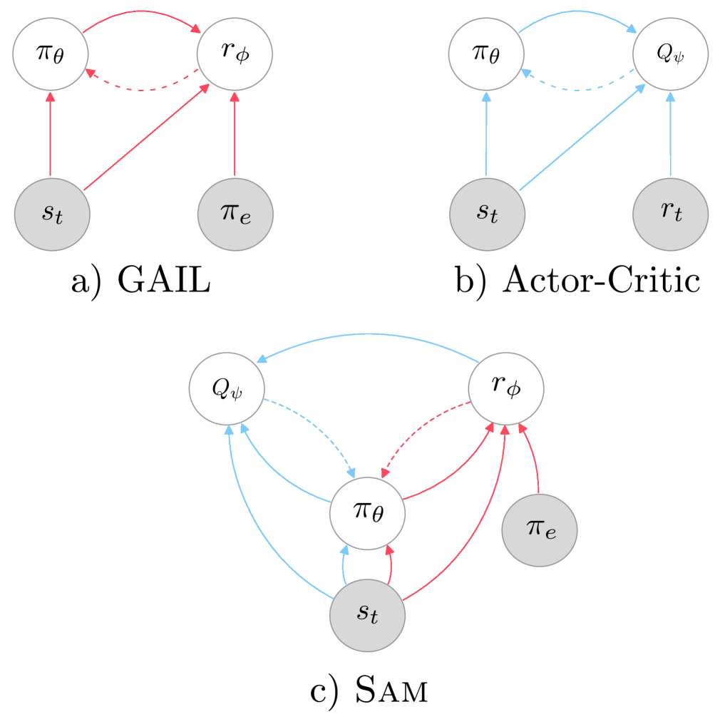
Figure 1: Inter-module relationships in different neural architectures (the scope of this figure was inspired from (Pfau and Vinyals,, 2016)). Modules with distinct loss functions are depicted with empty circles, while filled circles designate environmental entities. Solid and dotted arrows respectively represent (forward) flow of information and (backward) flow of gradient. a) Generative Adversarial Imitation Learning (Ho and Ermon,, 2016) b) Actor-Critic architecture (Sutton et al.,, 1999) c) Sam (this work). Note that in Sam, the critic takes in information from the reward module, while in the vanilla AC architecture, the critic receives the reward from the environment. The gradient flow from the critic to the reward module must however be sealed. Indeed, such a gradient flow would allow the policy to adjust its parameters to induce values of the reward which yield low TD residuals, hence preventing both critic and reward modules to be learned as intended.

As an off-policy method, Sam cycles through the following steps: i) the agent uses $\pi_{\theta}$ to interact with $\mathbb{M}^{+}$, ii) stores the experienced transitions $\mathcal{C}$ in a replay buffer $\mathcal{R}$, iii) updates the reward module $\phi$ with an equal mixture of uniformly sampled state-action pairs from $\mathcal{C}$ and $\tau_{e}$, iv) updates the reward module $\phi$ with an equal mixture of uniformly sampled state-action pairs from $\mathcal{R}$ and $\tau_{e}$, and v) updates the policy module $\theta$ and critic module $\psi$ with transitions sampled from $\mathcal{R}$. Note that while sampling uniformly from $\mathcal{C}$ (iii) gives states and actions distributed as $\rho^{\pi_{\theta}}$ and $\pi_{\theta}$ respectively (on-policy), sampling uniformly from $\mathcal{R}$ (iv) gives states and actions distributed as $\rho^{\beta}$ and $\beta$ respectively, where $\beta$ denotes the off-policy sampling mixture distribution corresponding to sampling transitions uniformly from the replay buffer. A more detailed description of the training procedure is laid out in the algorithm pseudo-code (Algorithm 1).

Reward

We introduce a reward network with parameter vector $\phi$, operating as the discriminator. The cross-entropy loss used to train the reward network is:

$$\mathbb{E}_{\pi_{\theta}}[-\log(1-D_{\phi}(s,a))] +\mathbb{E}_{\pi_{e}}[-\log D_{\phi}(s,a)]$$ (1)

$$+\lambda\mathfrak{R}_{\text{GP}}(\phi)$$ (2)

where $\mathfrak{R}_{\text{GP}}(\phi)$ is a penalty on the discriminator gradient, as introduced in (Gulrajani et al.,, 2017), Section 4. (Lucic et al.,, 2017) reports benefits from applying such regulariser to the non-saturated variant of the discriminator loss, although it was initially introduced for Wasserstein GANs (Arjovsky et al.,, 2017) in (Gulrajani et al.,, 2017). This penalty favours our method by further improving its stability.

The reward is defined as the negative of the generator loss. The later has been declined in many variants, which are thoroughly compared in (Lucic et al.,, 2017). We can therefore analogously define a synthetic reward for each of these forms. We go over and discuss major ones in supplementary material. Additionally, (Fu et al.,, 2018) proposes an extra variant in the context of IRL. In the remainder, we use $r_{\phi}(s_{t},a_{t})=-\log(1-D_{\phi}(s_{t},a_{t}))$ as synthetic reward. The reward network is trained, each iteration, first on the mini-batch most recently collected by $\pi_{\theta}$, then on mini-batches sampled from the replay buffer. Although (Pfau and Vinyals,, 2016) reports that using a replay buffer in GANs causes the generation to be poor, we do not seem to suffer the same detrimental effect in the continuous control tasks we tackle.

Critic

The loss optimised by the critic, noted $\ell(\psi)$, involves three components: i) a $1$-step Bellman residual $\ell_{1}(\psi)$, ii) a $n$-step Bellman residual $\ell_{n}(\psi)$, and iii) a weight decay regulariser $\mathfrak{R}_{\text{WD}}(\psi)$. A similar loss is employed in (Večerík et al.,, 2017) in the context of Reinforcement Learning from Demonstrations. While the authors use weight decay regularisers for both the policy and the critic, we restrain from decaying the policy’s weights since, in our setting, the policy plays a role in two distinct optimization problems. We do not apply a weight decay regulariser for the discriminator either, as it was proven to cause the Wasserstein GAN critic (name given to the discriminator in Wasserstein GANs) to diverge (Gulrajani et al.,, 2017).

We define the critic loss as follows:

$$\ell(\psi)=\ell_{1}(\psi)+\ell_{n}(\psi)+\nu\mathfrak{R}_{\text{WD}}(\psi)$$ (3)

where $\nu$ is a hyperparameter that determines how much decay is used. The losses i) and ii) are defined respectively based on the $1$-step and $n$-step lookahead versions of the Bellman equation,

$$\tilde{Q}_{\psi}^{1}(s_{t},a_{t}) \triangleq r_{\phi}(s_{t},a_{t})$$ (4)

$$+\gamma Q_{\psi}(s_{t+1},\mu_{\theta}(s_{t+1}))$$ (5)

$$\tilde{Q}_{\psi}^{n}(s_{t},a_{t}) \triangleq\sum_{k=0}^{n-1}\gamma^{k}r_{\phi}(s_{t+k},a_{t+k})$$ (6)

$$+\gamma^{n}Q_{\psi}(s_{t+n},\mu_{\theta}(s_{t+n}))$$ (7)

yielding the critic losses:

$$\ell_{1}(\psi)\triangleq\mathbb{E}_{s_{t}\sim\rho^{\beta},a_{t}\sim\beta}[(\tilde{Q}_{\psi}^{1}-Q_{\psi})^{2}(s_{t},a_{t})]$$ (8)

$$\ell_{n}(\psi)\triangleq\mathbb{E}_{s_{t}\sim\rho^{\beta},a_{t}\sim\beta}[(\tilde{Q}_{\psi}^{n}-Q_{\psi})^{2}(s_{t},a_{t})]$$ (9)

where $\mathbb{E}_{s_{t}\sim\rho^{\beta},,a_{t}\sim\beta}[\cdot]$ signifies that transitions are sampled from the replay buffer $\mathcal{R}$, using in effect the off-policy distribution $\beta$. Both $Q_{\psi}$ and $\tilde{Q}_{\psi}^{\cdot}$ ((5), (7)) depend on $\psi$, which might cause severe instability. In order to prevent the critic from diverging, we use separate target networks for both policy and critic ($\smash{\theta^{\prime}}$, $\smash{\psi^{\prime}}$) to calculate $\smash{\tilde{Q}_{\psi}^{\cdot}}$, which slowly track the learned parameters ($\theta$, $\psi$). In line with results exhibited in the recent ablation study (Rainbow (Hessel et al.,, 2017)) assessing the influence of the various add-ons of DQN (Mnih et al.,, 2013, 2015) on its performance, we studied the influence of two add-ons that were transposable to Sam: longer TD backups and replay prioritisation. $n$-step returns not only played a significant role in improving the sample complexity, but also had a positive influence on stability in the training regime. Prioritized Experience Replay (Schaul et al.,, 2016) however prevented Sam from consistently learning well-behaved policies. Being already prone to overfitting in its original setting (Schaul et al.,, 2016), we conjecture this phenomenon is amplified in our setting since the TD-errors, instrumental in the priority assignments, depend on rewards that are themselves learned. Uniform experience replay offers greater resilience against oversampling transitions that have wrongfully been assigned high synthetic rewards by the adversarially-trained reward module.

Policy

We update the policy $\mu_{\theta}$ so as to maximise the performance objective, defined as the expected return from the start state. To that end, the policy is updated by taking a gradient ascent step along:

$$\nabla_{\theta}^{(1)}J(\mu_{\theta}) \approx\mathbb{E}_{s_{t}\sim\rho^{\beta}}\left[\nabla_{\theta}Q_{\psi}(s_{t},\mu_{\theta}(s_{t}))\right]$$ (10)

$$=\mathbb{E}_{s_{t}\sim\rho^{\beta}}\left[\nabla_{\theta}\mu_{\theta}(s_{t})\nabla_{a}Q_{\psi}(s_{t},a)|_{a=\mu_{\theta}(s_{t})}\right]$$ (11)

where the partial derivative with respect to the state is ignored since we consider the model-free setting. This gradient estimation stems from the policy gradient theorem proved by (Silver et al.,, 2014), and points towards regions of the parameter space in which the policy displays high similarity with the demonstrator.

We model the synthetic reward as a parametrised function that takes a state and an action as inputs. As such, we can take the derivative of the reward with respect to $\theta$. By applying the chain rule, we obtain:

$$\nabla_{\theta}^{(2)}J(\mu_{\theta}) \approx\mathbb{E}_{s_{t}\sim\rho^{\beta}}\left[\nabla_{\theta}r_{\phi}(s_{t},\mu_{\theta}(s_{t}))\right]$$ (12)

$$=\mathbb{E}_{s_{t}\sim\rho^{\beta}}\left[\nabla_{\theta}\mu_{\theta}(s_{t})\nabla_{a}r_{\phi}(s_{t},a)|_{a=\mu_{\theta}(s_{t})}\right]$$ (13)

which constitutes another estimate of how to update the policy parameters $\theta$ to increase the similarity between the policy and the expert ((Sasaki and Kawaguchi,, 2018) employs a similar estimate). Each estimate of how well the agent is behaving, $r_{\phi}$ and $Q_{\psi}$, is trained via a different policy evaluation method, each presenting its own advantages. The first is updated by adversarial training, providing an accurate estimate of the immediate similarity with expert trajectories. The second is trained via TD learning, enabling longer propagation of rewards along trajectories and effectively tackling the credit assignment problem. While our formulation enables us to use either of these gradient estimates, $\nabla_{\theta}^{(1)}J(\mu_{\theta})$ is more suited to learn control policies in environments inducing delayed rewards. As the continuous control tasks we consider in this paper belong to this category, we use $\nabla_{\theta}^{(1)}J(\mu_{\theta})$ to update the policy module. While we could use a mixture of $\nabla_{\theta}^{(1)}J(\mu_{\theta})$ and $\nabla_{\theta}^{(2)}J(\mu_{\theta})$ we found that the latter had a detrimental effect on the former, as it prevented the policy to reason across timesteps, resulting in poor reward propagation.

Exploration

Deterministic policies have zero variance in their predictions for a given state, translating to no exploratory behaviour. The exploration problem is therefore treated independently from how the policy is modelled, by defining a stochastic policy $\pi_{\theta}$ from the learned deterministic policy $\mu_{\theta}$. In this work, we construct $\pi_{\theta}$ via the combination of two fundamentally different techniques: a) by applying an adaptive perturbation to the learned weights $\theta$ (exploration by noise-injection in parameter space (Plappert et al.,, 2018; Fortunato et al.,, 2017)) and b) by adding temporally-correlated noise sampled from a Ornstein-Uhlenbeck process $\mathbb{O}\mathbb{U}$ (Lillicrap et al.,, 2016), well-suited for control tasks involving inertia (e.g. simulated robotics and locomotion tasks). We denote the obtained policy by $\pi_{\theta}\triangleq\mu_{\tilde{\theta}}+\mathbb{O}\mathbb{U}$, where $\tilde{\theta}$ results from applying a) to $\theta$. When interacting with the environment, Sam samples from the conditional distribution $\pi_{\theta}$, and stores the collected transitions in the replay buffer $\mathcal{R}$. An interesting result is that the reward is adversarially trained on samples coming from the parameter-perturbed policy. Rather than causing severe divergence, it seems that it positively impacts the adversarial training procedure. This observation directly echoes noise-injection techniques from the GAN literature. The additive noise applied to the output of our policy (which plays the role of generator in our architecture) aligns with (Arjovsky and Bottou,, 2017) who add artificial noise to the inputs of the discriminator (although we do not perturb expert trajectories). Furthermore, perturbing $\mu_{\theta}$ in parameter space draws strong similarities with (Zhao et al.,, 2017), in which the authors add Gaussian noise to the layers of the generator.

Initialise replay buffer $\mathcal{R}$

Initialise network parameters ($\phi$, $\theta$, $\psi$)

Initialise target network parameters ($\theta^{\prime}$, $\psi^{\prime}$) as respective copies of ($\theta$, $\psi$)

for $\text{i}\in 1,\ldots,\text{i}_{\text{max}}$ do

       # Interact with environment

       # and store collected transitions

       for $\text{c}\in 1,\ldots,\text{c}_{\text{max}}$ do

             Interact with environment following $\pi_{\theta}$ and collect the experienced transitions in $\mathcal{C}$ augmented with synthetic rewards

             Store $\mathcal{C}$ in the replay buffer $\mathcal{R}$

       end for

      for $\text{t}\in 1,\ldots,\text{t}_{\text{max}}$ do

             # Update reward module

             for $\text{d}\in 1,\ldots,\text{d}_{\text{max}}$ do

                   Sample uniformly a minibatch $\mathcal{B}^{c}$ of state-action pairs pairs from $\mathcal{C}$

                   Sample uniformly a minibatch $\mathcal{B}_{e}^{c}$ of state-action pairs from the expert dataset $\tau_{e}$, with $|\mathcal{B}^{c}|=|\mathcal{B}_{e}^{c}|$

                   Update synthetic reward parameter $\phi$ with the equal mixture $\mathcal{B}^{c}\cup\mathcal{B}_{e}^{c}$ by following the gradient: $\hat{\mathbb{E}}_{\mathcal{B}^{c}}[\nabla_{\phi}\log(1-D_{\phi}(s,a))]+\hat{\mathbb{E}}_{\mathcal{B}_{e}^{c}}[\nabla_{\phi}\log D_{\phi}(s,a)]+\lambda\nabla_{\phi}\mathfrak{R}_{\text{GP}}(\phi)$

                   Sample uniformly a minibatch $\mathcal{B}^{d}$ of state-action pairs from $\mathcal{R}$

                   Sample uniformly a minibatch $\mathcal{B}_{e}^{d}$ of state-action pairs from the expert dataset $\tau_{e}$, with $|\mathcal{B}^{d}|=|\mathcal{B}_{e}^{d}|$

                   Update synthetic reward parameter $\phi$ with the equal mixture $\mathcal{B}^{d}\cup\mathcal{B}_{e}^{d}$ by following the gradient: $\hat{\mathbb{E}}_{\mathcal{B}^{d}}[\nabla_{\phi}\log(1-D_{\phi}(s,a))]+\hat{\mathbb{E}}_{\mathcal{B}_{e}^{d}}[\nabla_{\phi}\log D_{\phi}(s,a)]+\lambda\nabla_{\phi}\mathfrak{R}_{\text{GP}}(\phi)$

             end for

            # Update policy and critic modules

             for $\text{g}\in 1,\ldots,\text{g}_{\text{max}}$ do

                   Sample uniformly a minibatch $\mathcal{B}^{g}$ of transitions from $\mathcal{R}$

                   Update policy parameter $\theta$ by following the gradient: $\hat{\mathbb{E}}_{\mathcal{B}^{g}}[\nabla_{\theta}J(\mu_{\theta})]$

                   Update critic parameters $\psi$ by minimizing critic loss: $\hat{\mathbb{E}}_{\mathcal{B}^{g}}[\ell(\psi)]$

                   Update target network parameters ($\theta^{\prime}$, $\psi^{\prime}$) to slowly track ($\theta$, $\psi$), respectively

             end for

            

       end for

      

end for

Algorithm 1 Sample-efficient Adversarial Mimic

5 Results

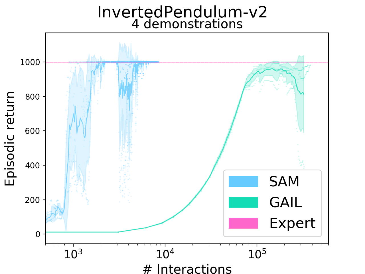
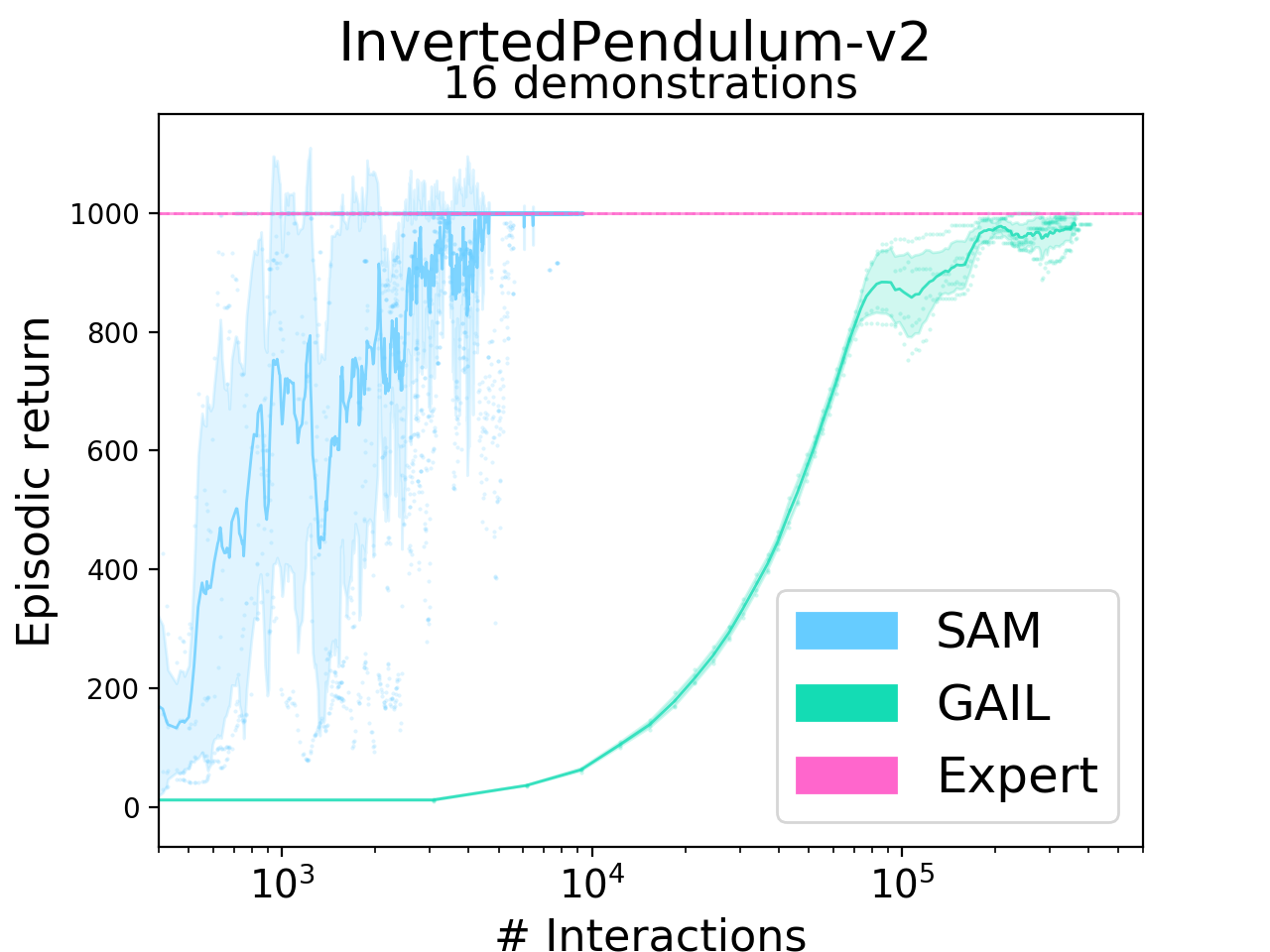
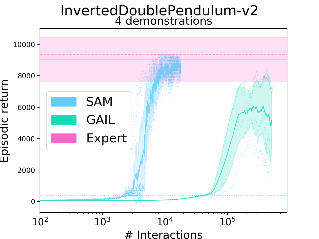
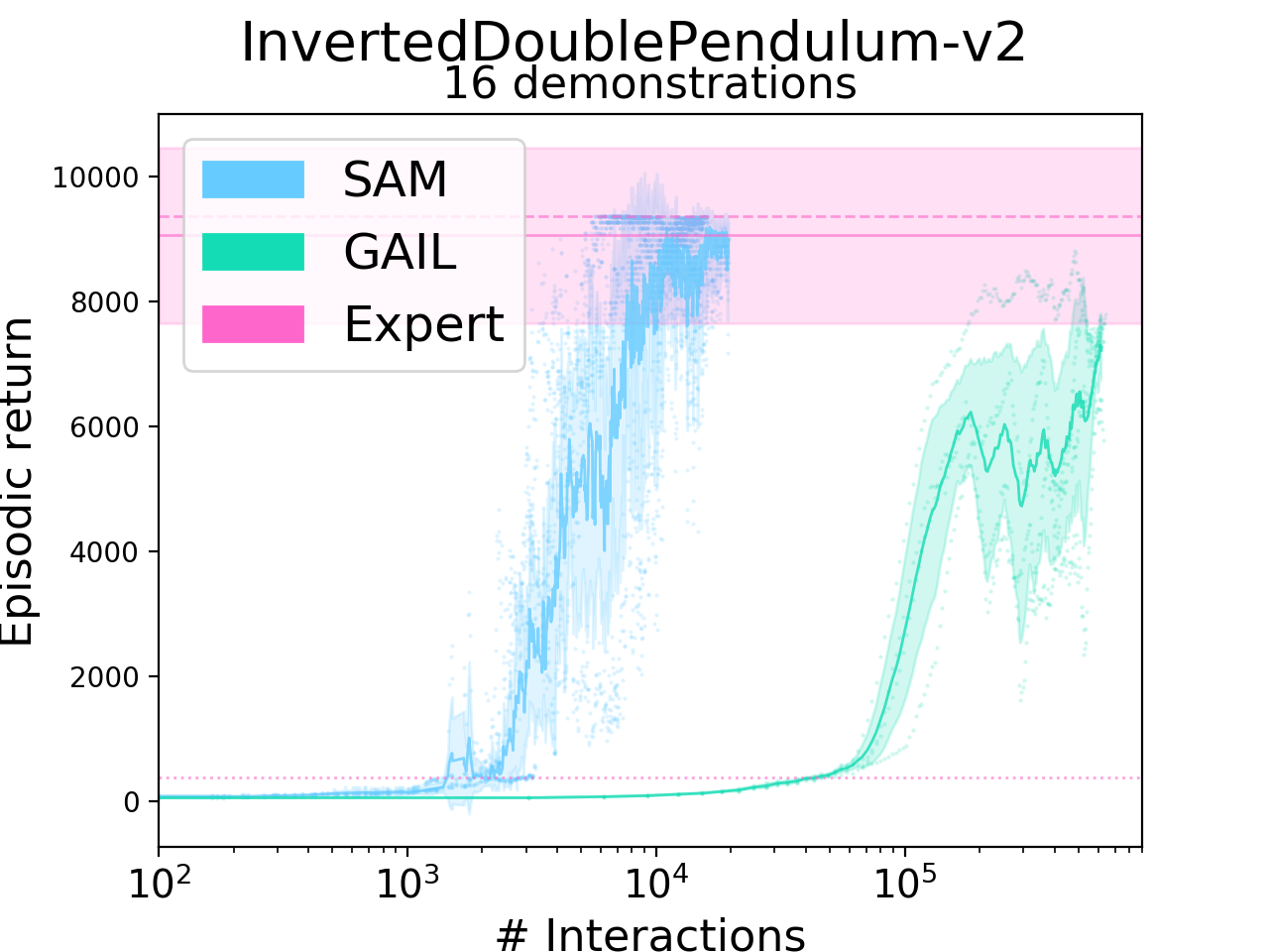
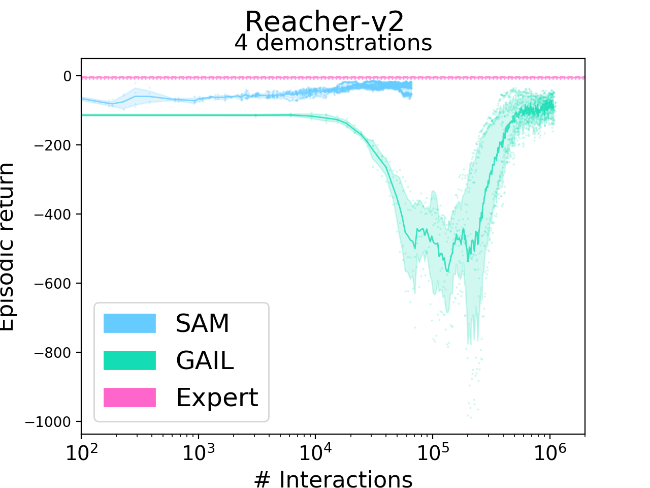
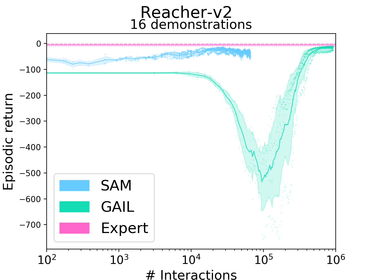
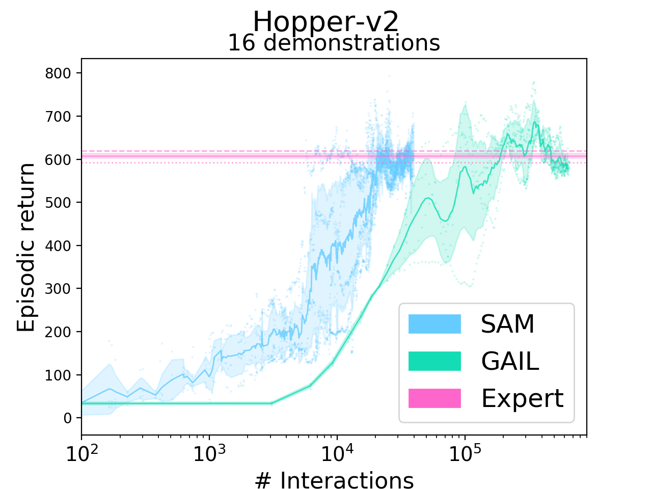
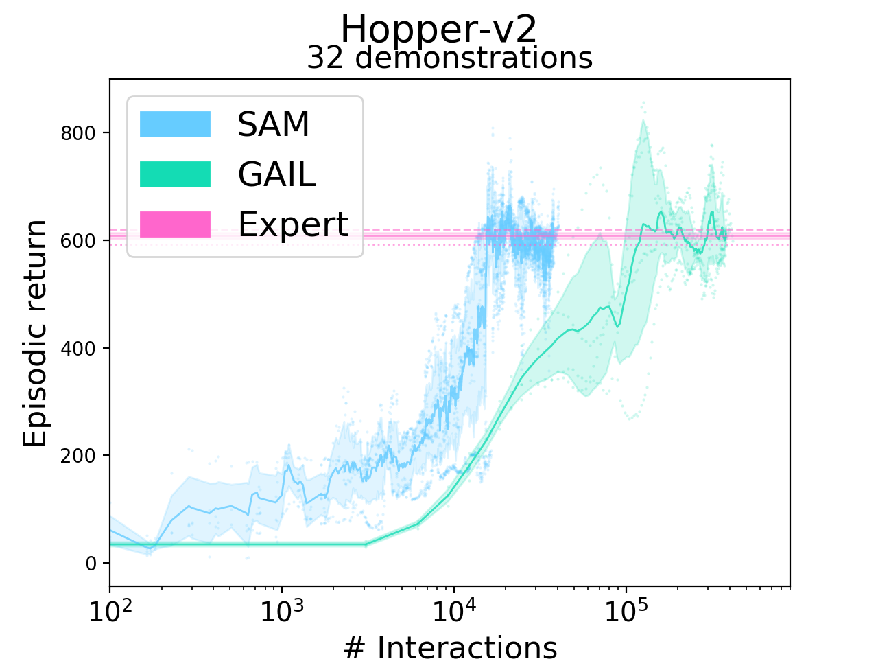
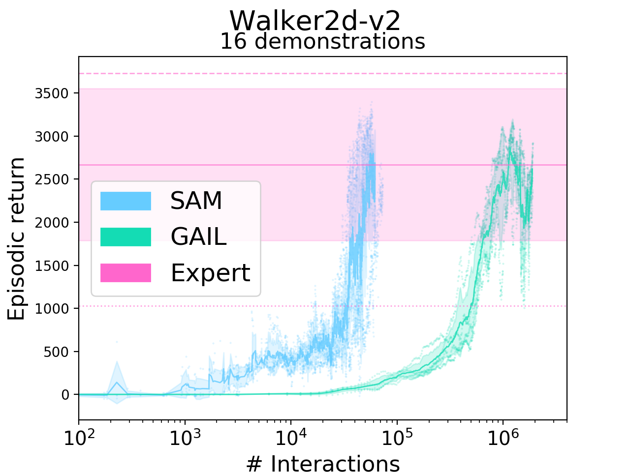
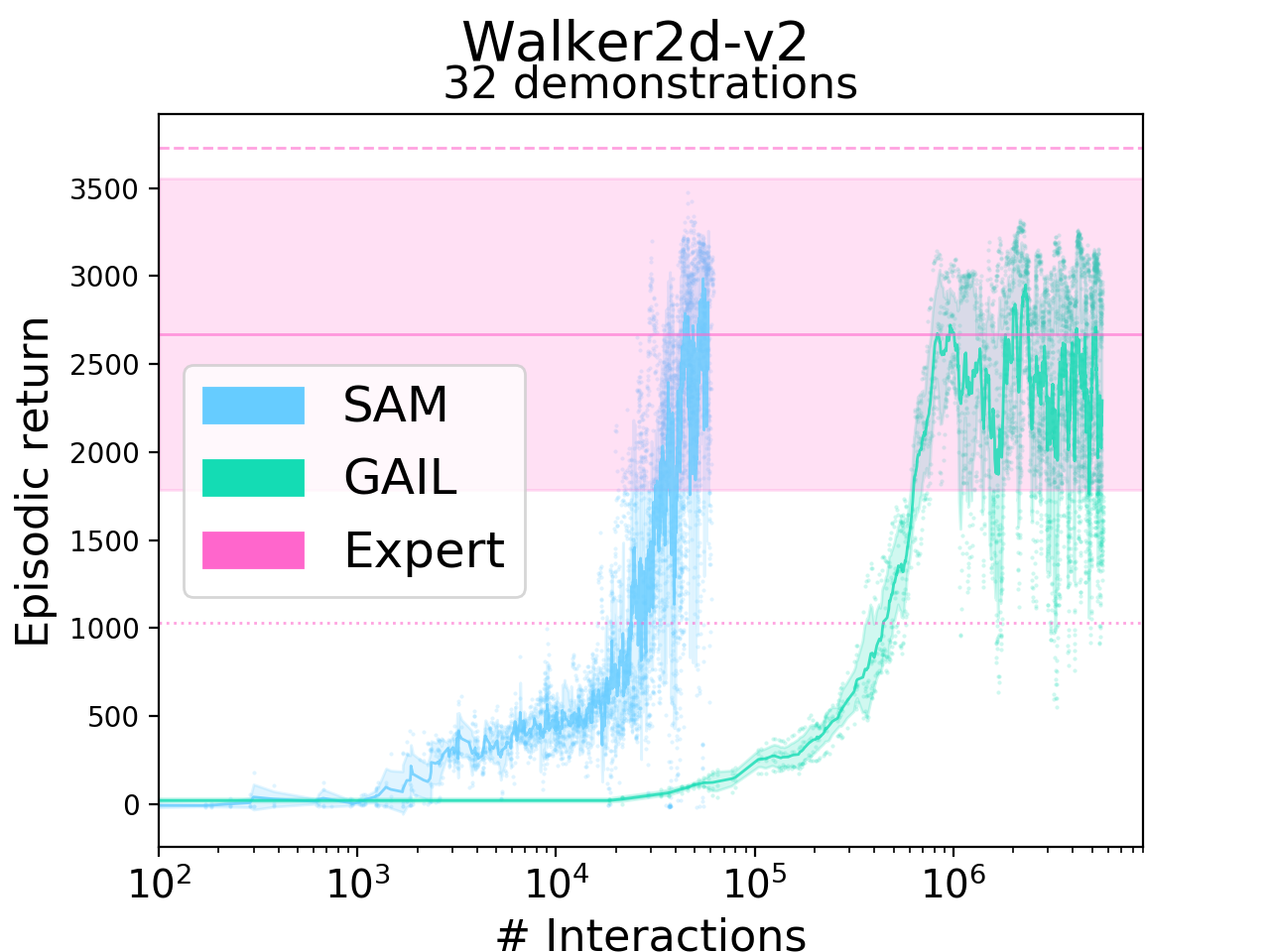
Figure 2: Performance comparison between Sam and GAIL in terms of episodic return. The horizontal axis depicts, in logarithmic scale, the number of interactions with the environment. While there is no ambiguity for GAIL, we used the unperturbed Sam policy $\mu_{\theta}$ (without parameter noise and additive action noise) to collect those returns during a per-iteration evaluation phase. The figure shows that our method has a considerably better sample-efficiency than GAIL in various continuous control tasks, often by several orders of magnitude. Red-colored lines and filled areas indicate the performance range of the expert demonstrations present in the training set. The meaning of the different line styles and colors is given in-text.

Our agents were trained in physics-based control environments, built with the MuJoCo physics engine (Todorov et al.,, 2012), and wrapped via the OpenAI Gym (Brockman et al.,, 2016) API. Tasks simulated in the environments range from legacy balance-oriented tasks to simulated robotics and locomotion tasks of various complexities. In this work, we consider the 5 following environments, ordered by increasing complexity (degrees of freedom in state and action spaces): InvertedPendulum, InvertedDoublePendulum, Reacher, Hopper, Walker2d. In the experiments presented in Figure 2, we explore how the performance of SAM and that of GAIL evolve as a function of the number of interactions they have with the environment.

For each environment, an expert was designed by training an agent for 10M timesteps using the Proximal Policy Optimization (PPO) algorithm (Schulman et al.,, 2017). The episode horizon (maximum episode length) was left to its default value per environment. We created a dataset of expert trajectories per environment. For every environment, we evaluated the performance of the agents when provided with various quantities of demonstrations, sampled for the demonstration dataset associated with the environment. We do so in order to explore how the two methods behave with respect to the number of demonstrations to which they are exposed. Both models are shown the same set of selected trajectories. We ensure that the two compared models are trained on exactly the same subset of extracted trajectories by training them with the same random seeds. We varied the cardinality of the set of selected trajectories as a function of the environment’s complexity. We ran every experiment on the same range of 4 random seeds, namely $\{0,1,2,3\}$. In Figure 2, we use scatter plots to visualise every episodic return, for every random seed. Solid blue and green lines represent the mean episodic return across the random seeds for the given number of interactions. The filled areas are confidence intervals around the solid lines, corresponding to a fixed fraction of the standard deviation around the mean for the given number of interactions. Every item coloured in red relates to the expert performance, for a given environment. The solid red line corresponds to the mean episodic return of the demonstrations present in the expert dataset associated with the given environment. The filled red region is a trust region whose width is equal to the standard deviation of returns in the expert dataset. The dotted line depicts the minimum return in the demonstration dataset while the dashed line represents the maximum. Having statistics about the demonstration datasets is particularly insightful when evaluating the results of experiments dealing with few demonstrations.

Every experiment runs with 4 parallel instantiations of the same model, initialised with different seeds. Each instantiation has its own interaction with the environment, its own replay buffer and its own optimisers. However, every iteration, the gradients are averaged per module across instantiations and the averaged gradients are distributed per module to every instantiation and immediately used to update the respective module parameters. Both Sam and GAIL experiments were run under this setting. This vertical scalability played a considerable role in speeding up training phases, equivalently for both models. Since every instantiation has its own random seed, the fairness of our performance comparison between Sam and GAIL is further strengthened (Henderson et al.,, 2017).

We used layer normalisation (Ba et al.,, 2016) in the policy module. Indeed, applying layer normalisation to every layer of the policy was instrumental in yielding better results, in line with the observations reported in (Plappert et al.,, 2018). To ensure symmetry within the actor-critic architecture, we also applied layer normalisation to the critic module. Pop-Art (van Hasselt et al.,, 2016) was also useful to our architecture as our learned reward would sometimes output scores of various magnitudes. Applying Pop-Art helped in overcoming the various scales. Finally, note that Sam and GAIL implementations use exactly the same discriminator implementation.

We provide architecture, hyperparameter, implementation, and other details in the supplementary material. We also provide video visualisations of learned policies at https://youtu.be/-nCsqUJnRKU, as well as the code associated with this work at https://github.com/lionelblonde/sam-tf.

The sample-efficiency we gain over GAIL is considerable: Sam needs one or two orders of magnitude less interactions with the environment to attain asymptotic expert performance. Note that the horizontal axis is scaled logarithmically. Additionally, we observe in Figure 2 that GAIL agents sometimes fall short of reaching the demonstrator’s asymptotic performance (e.g. Reacher and InverseDoublePendulum). While GAIL requires full traces of agent–environment interaction per iteration as it relies on Monte-Carlo estimates, Sam only requires a couple of transitions per iteration since it performs policy evaluation via Temporal Difference learning. Instead of sampling transitions from the environment, performing an update and discarding the transitions, Sam keeps experiential data in memory and can therefore leverage decorrelated transitions collected in previous iterations to perform an off-policy update. Our method therefore requires considerably fewer new samples (interactions) per iteration, as it can re-exploit the transitions previously experienced.

Since our approach trades interactions with the environment with replays with past experiences to extract more knowledge out of past interactions, echoing fictitious play in game theory, it generally takes a longer wall-clock time to train imitation policies. However, in real-world scenarios (e.g. robotic manipulation, autonomous cars), reducing the required interaction with the world is significantly more desirable, for safety and cost reasons.

6 Conclusion

In this work, we introduced a method, called Sample-efficient Adversarial Imitation Learning (Sam), that meaningfully overcomes one considerable drawback of GAIL (Ho and Ermon,, 2016): the number of agent–environment interactions it requires to learn expert-like policies. We demonstrate that our method shrinks the number of interactions by an order of magnitude, and sometimes more. Leveraging an off-policy procedure was key to that success.

References

- Abbeel and Ng, (2004) Abbeel, P. and Ng, A. Y. (2004). Apprenticeship Learning via Inverse Reinforcement Learning. In International Conference on Machine Learning (ICML).
- Arjovsky and Bottou, (2017) Arjovsky, M. and Bottou, L. (2017). Towards Principled Methods for Training Generative Adversarial Networks. In International Conference on Learning Representations (ICLR).
- Arjovsky et al., (2017) Arjovsky, M., Chintala, S., and Bottou, L. (2017). Wasserstein GAN.
- Ba et al., (2016) Ba, J. L., Kiros, J. R., and Hinton, G. E. (2016). Layer Normalization.
- Bagnell, (2015) Bagnell, J. A. (2015). An invitation to imitation. Technical report, Carnegie Mellon, Robotics Institute, Pittsburgh.
- Baram et al., (2017) Baram, N., Anschel, O., Caspi, I., and Mannor, S. (2017). End-to-End Differentiable Adversarial Imitation Learning. In International Conference on Machine Learning (ICML), pages 390–399.
- Billard et al., (2008) Billard, A., Calinon, S., Dillmann, R., and Schaal, S. (2008). Robot Programming by Demonstration. In Bruno, S. and Oussama, K., editors, Springer Handbook of Robotics, pages 1371–1394. Springer Berlin Heidelberg.
- Brockman et al., (2016) Brockman, G., Cheung, V., Pettersson, L., Schneider, J., Schulman, J., Tang, J., and Zaremba, W. (2016). OpenAI Gym.
- Finn et al., (2016) Finn, C., Christiano, P., Abbeel, P., and Levine, S. (2016). A Connection between Generative Adversarial Networks, Inverse Reinforcement Learning, and Energy-Based Models.
- Fortunato et al., (2017) Fortunato, M., Azar, M. G., Piot, B., Menick, J., Osband, I., Graves, A., Mnih, V., Munos, R., Hassabis, D., Pietquin, O., Blundell, C., and Legg, S. (2017). Noisy Networks for Exploration.
- Fu et al., (2018) Fu, J., Luo, K., and Levine, S. (2018). Learning Robust Rewards with Adversarial Inverse Reinforcement Learning. In International Conference on Learning Representations (ICLR).
- Goodfellow, (2017) Goodfellow, I. (2017). NIPS 2016 Tutorial: Generative Adversarial Networks.
- Goodfellow et al., (2014) Goodfellow, I., Pouget-Abadie, J., Mirza, M., Xu, B., Warde-Farley, D., Ozair, S., Courville, A., and Bengio, Y. (2014). Generative Adversarial Nets. In Neural Information Processing Systems (NIPS), pages 2672–2680.
- Gu et al., (2016) Gu, S., Lillicrap, T., Ghahramani, Z., Turner, R. E., and Levine, S. (2016). Q-Prop: Sample-Efficient Policy Gradient with An Off-Policy Critic. In International Conference on Learning Representations (ICLR).
- Gulrajani et al., (2017) Gulrajani, I., Ahmed, F., Arjovsky, M., Dumoulin, V., and Courville, A. (2017). Improved Training of Wasserstein GANs. In Neural Information Processing Systems (NIPS).
- Hausman et al., (2017) Hausman, K., Chebotar, Y., Schaal, S., Sukhatme, G., and Lim, J. (2017). Multi-Modal Imitation Learning from Unstructured Demonstrations using Generative Adversarial Nets. In Neural Information Processing Systems (NIPS).
- Henderson et al., (2017) Henderson, P., Islam, R., Bachman, P., Pineau, J., Precup, D., and Meger, D. (2017). Deep Reinforcement Learning that Matters.
- Hessel et al., (2017) Hessel, M., Modayil, J., van Hasselt, H., Schaul, T., Ostrovski, G., Dabney, W., Horgan, D., Piot, B., Azar, M., and Silver, D. (2017). Rainbow: Combining Improvements in Deep Reinforcement Learning.
- Ho and Ermon, (2016) Ho, J. and Ermon, S. (2016). Generative Adversarial Imitation Learning. In Neural Information Processing Systems (NIPS).
- Ho et al., (2016) Ho, J., Gupta, J. K., and Ermon, S. (2016). Model-Free Imitation Learning with Policy Optimization.
- Jang et al., (2017) Jang, E., Gu, S., and Poole, B. (2017). Categorical Reparameterization with Gumbel-Softmax. In International Conference on Learning Representations (ICLR).
- Kingma and Ba, (2014) Kingma, D. P. and Ba, J. (2014). Adam: A Method for Stochastic Optimization.
- Kingma and Welling, (2013) Kingma, D. P. and Welling, M. (2013). Auto-Encoding Variational Bayes.
- Kostrikov et al., (2018) Kostrikov, I., Agrawal, K. K., Levine, S., and Tompson, J. (2018). Addressing Sample Inefficiency and Reward Bias in Inverse Reinforcement Learning.
- Kuefler and Kochenderfer, (2017) Kuefler, A. and Kochenderfer, M. J. (2017). Burn-In Demonstrations for Multi-Modal Imitation Learning.
- Levine et al., (2011) Levine, S., Popovic, Z., and Koltun, V. (2011). Nonlinear Inverse Reinforcement Learning with Gaussian Processes. In Neural Information Processing Systems (NIPS), pages 19–27.
- Li et al., (2017) Li, Y., Song, J., and Ermon, S. (2017). InfoGAIL: Interpretable Imitation Learning from Visual Demonstrations. In Neural Information Processing Systems (NIPS).
- Lillicrap et al., (2016) Lillicrap, T. P., Hunt, J. J., Pritzel, A., Heess, N., Erez, T., Tassa, Y., Silver, D., and Wierstra, D. (2016). Continuous control with deep reinforcement learning. In International Conference on Learning Representations (ICLR).
- Lucic et al., (2017) Lucic, M., Kurach, K., Michalski, M., Gelly, S., and Bousquet, O. (2017). Are GANs Created Equal? A Large-Scale Study.
- Maddison et al., (2017) Maddison, C. J., Mnih, A., and Teh, Y. W. (2017). The Concrete Distribution: A Continuous Relaxation of Discrete Random Variables. In International Conference on Learning Representations (ICLR).
- Mnih et al., (2013) Mnih, V., Kavukcuoglu, K., Silver, D., Graves, A., Antonoglou, I., Wierstra, D., and Riedmiller, M. (2013). Playing Atari with Deep Reinforcement Learning.
- Mnih et al., (2015) Mnih, V., Kavukcuoglu, K., Silver, D., Rusu, A. A., Veness, J., Bellemare, M. G., Graves, A., Riedmiller, M., Fidjeland, A. K., Ostrovski, G., Petersen, S., Beattie, C., Sadik, A., Antonoglou, I., King, H., Kumaran, D., Wierstra, D., Legg, S., and Hassabis, D. (2015). Human-level control through deep reinforcement learning. Nature, 518(7540):529–533.
- Ng et al., (1999) Ng, A. Y., Harada, D., and Russell, S. (1999). Policy invariance under reward transformations: Theory and application to reward shaping. In International Conference on Machine Learning (ICML), pages 278–287.
- Pfau and Vinyals, (2016) Pfau, D. and Vinyals, O. (2016). Connecting Generative Adversarial Networks and Actor-Critic Methods.
- Plappert et al., (2018) Plappert, M., Houthooft, R., Dhariwal, P., Sidor, S., Chen, R. Y., Chen, X., Asfour, T., Abbeel, P., and Andrychowicz, M. (2018). Parameter Space Noise for Exploration. In International Conference on Learning Representations (ICLR).
- Pomerleau, (1989) Pomerleau, D. (1989). ALVINN: An Autonomous Land Vehicle in a Neural Network. In Neural Information Processing Systems (NIPS), pages 305–313.
- Pomerleau, (1990) Pomerleau, D. (1990). Rapidly Adapting Artificial Neural Networks for Autonomous Navigation. In Neural Information Processing Systems (NIPS), pages 429–435.
- Ross and Bagnell, (2010) Ross, S. and Bagnell, J. A. (2010). Efficient Reductions for Imitation Learning. In International Conference on Artificial Intelligence and Statistics (AISTATS), pages 661–668. jmlr.org.
- Ross et al., (2011) Ross, S., Gordon, G. J., and Bagnell, J. A. (2011). A Reduction of Imitation Learning and Structured Prediction to No-Regret Online Learning. In International Conference on Artificial Intelligence and Statistics (AISTATS), pages 627–635. jmlr.org.
- Sasaki and Kawaguchi, (2018) Sasaki, F. and Kawaguchi, A. (2018). Deterministic Policy Imitation Gradient Algorithm.
- Schaul et al., (2016) Schaul, T., Quan, J., Antonoglou, I., and Silver, D. (2016). Prioritized Experience Replay. In International Conference on Learning Representations (ICLR).
- Schulman et al., (2015) Schulman, J., Levine, S., Moritz, P., Jordan, M. I., and Abbeel, P. (2015). Trust Region Policy Optimization. In International Conference on Machine Learning (ICML).
- Schulman et al., (2017) Schulman, J., Wolski, F., Dhariwal, P., Radford, A., and Oleg, K. (2017). Proximal Policy Optimization Algorithms.
- Silver et al., (2014) Silver, D., Lever, G., Heess, N., Degris, T., Wierstra, D., and Riedmiller, M. (2014). Deterministic Policy Gradient Algorithms. In International Conference on Machine Learning (ICML), pages 387–395.
- Sutton and Barto, (1998) Sutton, R. S. and Barto, A. G. (1998). Reinforcement Learning: An Introduction.
- Sutton et al., (1999) Sutton, R. S., McAllester, D. A., Singh, S. P., and Mansour, Y. (1999). Policy Gradient Methods for Reinforcement Learning with Function Approximation. In Neural Information Processing Systems (NIPS), pages 1057–1063.
- Syed et al., (2008) Syed, U., Bowling, M., and Schapire, R. E. (2008). Apprenticeship Learning Using Linear Programming. In International Conference on Machine Learning (ICML), pages 1032–1039.
- Syed and Schapire, (2008) Syed, U. and Schapire, R. E. (2008). A Game-Theoretic Approach to Apprenticeship Learning. In Neural Information Processing Systems (NIPS), pages 1449–1456.
- Todorov et al., (2012) Todorov, E., Erez, T., and Tassa, Y. (2012). MuJoCo: A physics engine for model-based control. In IEEE/RSJ International Conference on Intelligent Robots and Systems (IROS), pages 5026–5033.
- van Hasselt et al., (2016) van Hasselt, H., Guez, A., Hessel, M., Mnih, V., and Silver, D. (2016). Learning values across many orders of magnitude.
- Večerík et al., (2017) Večerík, M., Hester, T., Scholz, J., Wang, F., Pietquin, O., Piot, B., Heess, N., Rothörl, T., Lampe, T., and Riedmiller, M. (2017). Leveraging Demonstrations for Deep Reinforcement Learning on Robotics Problems with Sparse Rewards.
- Wang et al., (2016) Wang, Z., Bapst, V., Heess, N., Mnih, V., Munos, R., Kavukcuoglu, K., and de Freitas, N. (2016). Sample Efficient Actor-Critic with Experience Replay.
- Zhao et al., (2017) Zhao, J., Mathieu, M., and LeCun, Y. (2017). Energy-based Generative Adversarial Network. In International Conference on Learning Representations (ICLR).