Measuring nonclassicality of bosonic field quantum states via operator ordering sensitivity

Abstract.

We introduce a new distance-based measure for the nonclassicality of the states of a bosonic field, which outperforms the existing such measures in several ways. We define for that purpose the operator ordering sensitivity of the state which evaluates the sensitivity to operator ordering of the Renyi entropy of its quasi-probabilities and which measures the oscillations in its Wigner function. Through a sharp control on the operator ordering sensitivity of classical states we obtain a precise geometric image of their location in the density matrix space allowing us to introduce a distance-based measure of nonclassicality. We analyse the link between this nonclassicality measure and a recently introduced quantum macroscopicity measure, showing how the two notions are distinct.

1. Introduction

Questions arising in quantum information theory and in quantum chaos drive a continued interest in the exploration of the quantum-classical boundary. There is in this context a need for efficient criteria to determine the strength of the diverse nonclassical features of quantum states, such as: their Titulaer-Glauber nonclassicality [1, 2, 3, 4, 5, 6, 7, 8, 9, 10, 11, 12, 13, 14, 15, 16, 17, 18, 19, 20, 21, 22, 23], their degree of coherence and macroscopic nature [24, 25, 26, 27, 28, 29, 30, 31, 32, 33, 34, 35], their degree of entanglement in multi-partite systems, their entanglement potential for mono-partite systems [14, 20], their semi-classical breaking times in quantum chaos [36, 37], and the links between these notions. In this paper we investigate the nonclassicality question for systems described with bosonic variables. The well established definition of a Titulaer-Glauber classical state in this context is that it is a statistical mixture of coherent states, or equivalently, that its Glauber-Sudarshan $P$-function defines a probability on phase space [1]. Otherwise, it is nonclassical. In this paper, the term “nonclassical” will always be used in this precise sense. The two main issues in this respect are the identification of nonclassicality witnesses, or criteria, that allow to establish if a given state is nonclassical and the definition of quantitative measures of nonclassicality, that allow to say how nonclassical a state is.

Indeed, a direct analysis of the $P$-function is rarely feasible because for many states the $P$-function is neither theoretically, nor experimentally readily accessible. Consequently, to test for nonclassicality, various sufficient and more easily verified criteria have been designed. Some generalize the well-known quantum optics criteria such as the negativity of the Mandel parameter, which detects sub-Poissonian photon statistics, and of the degree of squeezing [7, 12, 18]. Others involve the negativity of the Wigner function [6, 9, 13], the entanglement potential of the state [14], or the minimal number of coherent states in terms of which one can write it as a superposition (See [20, 23] and references therein). While they capture various aspects of nonclassicality, they do not furnish a nonclassicality measure. An alternative approach is to use a distance between a given state and the set ${\mathcal{C}}$ of all classical states as a nonclassicality measure. This idea was pursued using the trace norm [3, 4, 22], the Hilbert-Schmidt norm [10], and the Bures distance [11]. It has been argued however that the resulting nonclassicality measure depends on the arbitrariness in the choice of norm [19]. Also, computing these distances has been possible only in very few cases, and even determining useful bounds on the nonclassicality has proven difficult [14, 23, 22].

We propose a distance-based measure of nonclassicality avoiding those drawbacks. We first construct a specifically adapted Hilbert norm on the density operators, whose square we refer to as the “operator ordering sensitivity” (OS) of the state $\rho$ (see (6) and (10)). It measures the sensitivity of the Renyi entropy of its quasi-probability distributions to operator ordering, an eminently nonclassical notion. We show the OS provides a simple and efficient sufficient condition for nonclassicality (see (6)) that is also necessary for pure states. Furthermore, as the square of a norm, the OS induces a distance ${\mathcal{N}}(\rho)$ from $\rho$ to the set ${\mathcal{C}}$ of all classical states that we propose as a new measure of nonclassicality (see (11)).

We will establish that the OS of $\rho$ yields a good approximation of the nonclassicality distance $\mathcal{N}(\rho)$, that it captures the intuitive physical ideas underlying nonclassicality well, and that it can often be more easily determined than existing criteria.

Another feature of the quantum-classical boundary is “quantum macroscopicity” which, loosely speaking, evaluates the degree to which a quantum state is the superposition of macroscopically distinct states. In absence of a generally agreed upon definition, various measures of quantum macroscopicity have been proposed [24, 25, 27, 26, 31, 33, 32, 34]. We will compare a proposal based on the quantum Fisher information to the nonclassicality measure ${\mathcal{N}}(\rho)$ and explain the relation between nonclassicality and quantum macroscopicity.

2. Ordering sensitivity: a nonclassicality witness

For ease of notation, we shall concentrate on one-dimensional systems, characterized by an annihilation-creation operator pair $a,a^{\dagger}$. We introduce the $s$-ordered quasi-probabilities $W_{s}(\alpha)$ of a state with density matrix $\rho$ following [38]. Let

$$\chi_{s}(\xi)=\exp\left(s\frac{|\xi|^{2}}{2}\right)\chi_{0}(\xi),\quad\chi_{0}(\xi)=\mathrm{Tr}\rho D(\xi),$$

where $D(\xi)=\exp(\xi a^{\dagger}-\xi^{*}a)$. Then

$$W_{s}(\alpha) = \frac{1}{\pi^{2}}\int\chi_{s}(\xi)\exp(\xi^{*}\alpha-\xi\alpha^{*})\mathrm{d}^{2}\xi.$$ (1)

Here $W_{0}(\alpha)$ is the Wigner function of $\rho$, $W_{1}(\alpha)$ its Glauber-Sudarshan $P$-function and $W_{-1}(\alpha)$ its Husimi function. We refer to $\chi_{s}(\xi)$ as the characteristic function of $W_{s}(\alpha)$. Then

$$\partial_{s}W_{s}(\alpha)=-\frac{1}{8}\Delta_{\alpha}W_{s}(\alpha).$$ (2)

Here $\alpha=\alpha_{1}+i\alpha_{2}\in\mathbb{C}$ and $\Delta_{\alpha}=\partial_{\alpha_{1}}^{2}+\partial_{\alpha_{2}}^{2}$, so that $W_{s}(\alpha)$ is a solution of a backward diffusion equation, in which $s$ plays the role of the time, a crucial observation for what follows. Since $\operatorname{Tr}\rho=1$, one has in particular $\int W_{s}(\alpha){\mathrm{d}}^{2}\alpha=1,$ which, together with the fact that $W_{s}(\alpha)$ is real valued but not necessarily nonnegative, explains the terminology “quasi-probability distribution.”

The Wigner function of $\rho$ is a continuous and square integrable function [39], meaning that $\|W_{0}\|_{2}^{2}:=\int|W_{0}|^{2}(\alpha){\mathrm{d}}^{2}\alpha<+\infty.$ For $s<0$, $W_{s}(\alpha)$ still has this property and actually becomes a smooth function, since it is the solution of a backward diffusion equation. For $s>0$, on the other hand, $W_{s}(\alpha)$, and in particular $P$, may develop strong singularities. Each single $W_{s}(\alpha)$ contains all information about $\rho$, which can in principle be reconstructed from it [38].

Following [1, 2, 40], we say a quantum state with density matrix $\rho$ is classical when the $P$-function of $\rho$ is a probability on the phase space $\mathbb{C}$. Below, we first establish a sufficient condition for a state $\rho$ to be nonclassical based on its ordering sensitivity ${S_{\mathrm{o}}}(\rho)$, which measures the variation in the quasi-probability distributions $W_{s}(\alpha)$ of the $\rho$, for $s$ close to $0$: see (6).

For that purpose, we introduce the $s$-ordered entropy of $\rho$:

$$H(s,\rho)=-\ln(\pi\|W_{s}\|_{2}^{2}).$$ (3)

This terminology is motivated by the observation that, when $W_{s}\geq 0$, it defines a bona fide probability. $H(s,\rho)$ is then the (second order) Renyi entropy of that probability, one of many possible measures of its uncertainty or unpredictability. A strongly localized or concentrated probability distribution corresponds to a low degree of uncertainty and a strongly negative Renyi entropy. Conversely, when a probability distribution is very much spread out, its Renyi entropy is large and positive. For $s=0$, $H(0,\rho)=-\ln\mathrm{Tr}\rho^{2}\geq 0$ has a direct physical interpretation: it is the logarithm of the purity $\mathcal{P}=\mathrm{Tr}\rho^{2}$ of $\rho$, and is in fact the Renyi entropy of its eigenvalues. It reaches its minimal value $0$ for pure states. Note that, from (2) one finds

$$H^{\prime}(s,\rho)=\frac{1}{4}\frac{\langle W_{s},\Delta W_{s}\rangle}{\parallel W_{s}\parallel_{2}^{2}}=-\frac{1}{4}\frac{\parallel\nabla W_{s}\parallel_{2}^{2}}{\parallel W_{s}\parallel_{2}^{2}}\leq 0.$$ (4)

Hence $H$ is a decreasing function of $s$, reflecting the fact that $W_{s}(\alpha)$ solves a backward diffusion equation leading to an increase in entropy backward in the “time” $s$ and a decrease forward in time. Taking a further derivative one easily sees $H^{\prime\prime}(\rho,s)\leq 0$ so that $H$ is concave in $s$.

Our main tool for the characterization of the nonclassicality of quantum states is the following bound on $H^{\prime}$.
Theorem. If $\rho$ is a classical state, then

$$0\leq-(1-s)H^{\prime}(s,\rho)\leq 1,\quad-1\leq s<1.$$ (5)

The proof is given in Appendix A and relies on (2). The upper bound $1$ is sharp, since one easily checks that, for coherent states, $H^{\prime}(s,|\alpha\rangle\langle\alpha|)=(s-1)^{-1}$. The lower bound follows from (4). By evaluating (5) at $s=0$, we infer the following sufficient condition for nonclassicality of $\rho$:

$${S_{\mathrm{o}}}(\rho):=-H^{\prime}(0,\rho)>1\Rightarrow\rho\ \text{is nonclassical}.$$ (6)

We call ${S_{\mathrm{o}}}(\rho)$ the ordering sensitivity (OS) of $\rho$. It measures the change in the $s$-ordered entropy of $\rho$, and hence the change in $W_{s}(\alpha)$, as $s$ varies close to $s=0$. This terminology is justified because different values of $s$ correspond to different operator orderings in the quantization procedure [41, 38]. The condition ${S_{\mathrm{o}}}(\rho)>1$ can hence be paraphrased by saying that the state $\rho$ is strongly ordering sensitive and (6) says this implies the state is not classical, in agreement with “operator ordering” as a typical quantum feature. This provides a first argument in favour of ${S_{\mathrm{o}}}(\rho)$ as a nonclassicality probe.

A second argument comes from the observation that $\nabla W_{0}$ probes the oscillations and short range structures of $W_{0}$, associated in particular with interference fringes and with the negativity of $W_{0}$. Hence, (4) implies ${S_{\mathrm{o}}}(\rho)$ provides a measure of such features. The normalization by $\|W_{0}\|^{2}$ ensures that it is the frequency of the oscillations rather than their amplitude that is measured. Since interference fringes are a hallmark of quantum mechanics, physical intuition suggests large values of ${S_{\mathrm{o}}}(\rho)$ are associated to a strongly nonclassical nature of the state. A contrario, if $\rho$ is a classical state then, setting $s=0$ in (5) and using (4), one finds ${S_{\mathrm{o}}}(\rho)\leq 1$ or

$$\|\nabla W_{0}\|_{2}^{2}\leq\frac{4}{\pi}\operatorname{Tr}\rho^{2}.$$ (7)

Hence, for classical states, these oscillations in the Wigner distribution are purity limited. The less pure a classical state, the smaller they are.

Equation (4) therefore links two quantum phenomena: the sensitivity of $W_{s}(\alpha)$ to the operator ordering parameter $s$ and the oscillations of $W_{s}(\alpha)$ at fixed $s$. The quantity $\|\nabla W_{0}\|^{2}/\|W_{0}\|^{2}$ has been used previously in quantum chaos studies [36, 37] and both $\|\nabla W_{0}\|^{2}/\|W_{0}\|^{2}$ and $\|\nabla W_{0}\|^{2}$ have been proposed as measures of “quantum macroscopicity” [25, 26, 27], but their relevance for that latter purpose has been contested [34] (see Section 5 and Appendix D for details.) Our results above reinterpret $\|\nabla W_{0}\|^{2}/\|W_{0}\|^{2}$ as the OS of the state and show it provides a nonclassicality witness. We will see it forms the basis for the construction of a nonclassicality measure.

Thirdly, we consider the behaviour of the OS when the system interacts with a thermal bath with mean photon number $\langle n\rangle$. We use a simple input-output model [14, 15] that can alternatively be interpreted as the action of a beam splitter [42]. The system, initially in the state $\rho_{\mathrm{in}}$, ends up in the state $\rho_{\mathrm{out}}$ after interaction with the bath, characterized by an efficiency $0\leq\lambda\leq 1$, where

$$\chi_{{\mathrm{out},1}}(\xi)=\chi_{\mathrm{in},1}(\sqrt{\lambda}\xi)\exp(-(1-\lambda)\langle n\rangle|\xi|^{2}).$$

As a result, with $\overline{s}=1+\lambda^{-1}((s-1)-2(1-\lambda)\langle n\rangle)\leq 1$,

$$W_{s,\mathrm{out}}(\alpha)=\lambda^{-1}W_{\overline{s},\mathrm{in}}(\frac{\alpha}{\sqrt{\lambda}}).$$

It follows that ${S_{\mathrm{o}}}(\rho_{\mathrm{out}})=-\lambda^{-1}H^{\prime}(\overline{s},\rho_{\mathrm{in}})$, with $\overline{s}=1-\lambda^{-1}(1+2(1-\lambda)\langle n\rangle)<0.$ Since $-H^{\prime}$ is a non-decreasing function of $s$, this yields ${S_{\mathrm{o}}}(\rho_{\mathrm{out}})\leq\lambda^{-1}{S_{\mathrm{o}}}(\rho_{\mathrm{in}})$. For $\lambda$ close to $1$ and $\langle n\rangle$ large enough, this shows that ${S_{\mathrm{o}}}(\rho_{\mathrm{out}})$ is lower than or equal to ${S_{\mathrm{o}}}(\rho_{\mathrm{in}})$. More precisely, in the weak coupling limit $\lambda\to 1$ and $(1-\lambda)\langle n\rangle\to\overline{e}$, this yields

$$\lim_{\lambda\to 1}{S_{\mathrm{o}}}(\rho_{\mathrm{out}})=-H^{\prime}(-2\overline{e},\rho_{\mathrm{in}})\leq{S_{\mathrm{o}}}(\rho_{\mathrm{in}}).$$

Since noisy environments destroy the quantal nature of states, this is again compatible with the interpretation of ${S_{\mathrm{o}}}(\rho)$ as an indicator of the level of nonclassicality of $\rho$, a point further developed below, see (11)-(12). In fact, the above equation shows that, the noisier the environment (large $\overline{e}$), the more it decreases ${S_{\mathrm{o}}}(\rho)$ and hence the nonclassicality of the initial state.

A final argument in favour of the pertinence of ${S_{\mathrm{o}}}(\rho)$ as a nonclassicality probe comes from the analysis of ${S_{\mathrm{o}}}(\rho)$ for pure states $\rho=|\psi\rangle\langle\psi|$. In that case, (10) below implies

$${S_{\mathrm{o}}}(\rho) = \big{\langle}(Q-\langle Q\rangle)^{2}\big{\rangle}+\big{\langle}(P-\langle P\rangle)^{2}\big{\rangle}$$ (8)

$$= 2\langle(a^{\dagger}-\langle a^{\dagger}\rangle)(a-\langle a\rangle)\rangle+1.$$

Here $Q=\frac{1}{\sqrt{2}}(a^{\dagger}+a)$, $P=\frac{i}{\sqrt{2}}(a^{\dagger}-a)$. This shows that for pure states the ordering sensitivity ${S_{\mathrm{o}}}(\rho)$ captures the intuitive idea that they are strongly nonclassical when they have a large uncertainty. Indeed, in classical mechanics pure states are identified with points in phase space and as such display no uncertainty, whereas in quantum mechanics, pure states must have uncertainty, of which ${S_{\mathrm{o}}}(\rho)$ is a natural measure. The uncertainty principle implies ${S_{\mathrm{o}}}(\rho)$ is larger than or equal to $1$ if $\rho$ is pure; it is equal to one only if $|\psi\rangle$ is a coherent state. Equations (5) and (8) therefore provide an alternative proof of the known fact that the only pure classical states are the coherent states [2]. It follows that the condition ${S_{\mathrm{o}}}(\rho)>1$ is both necessary and sufficient for the nonclassicality of pure states. We will now show how to use ${S_{\mathrm{o}}}(\rho)$ to construct a nonclassicality measure, thereby extending these ideas to mixed states.

3. A new nonclassicality measure

We have seen the ordering sensitivity ${S_{\mathrm{o}}}$ provides a sufficient condition for nonclassicality which is also necessary for pure states. We now construct, using ${S_{\mathrm{o}}}$, a nonclassicality measure for all states. For that purpose, we first interpret ${S_{\mathrm{o}}}$ geometrically. We define, for two operators $A,B$ with finite trace,

$$\langle A,B\rangle=\frac{1}{2}\operatorname{Tr}\left([A^{\dagger},Q][Q,B]+[A^{\dagger},P][P,B]\right).$$ (9)

This expression is linear in $B$, anti-linear in $A$, and positive when $B=A$. We will set ${\left|\kern-1.07639pt\left|\kern-1.07639pt\left|A\right|\kern-1.07639pt\right|\kern-1.07639pt\right|}=\langle A,A\rangle^{1/2}.$ If ${\left|\kern-1.07639pt\left|\kern-1.07639pt\left|A\right|\kern-1.07639pt\right|\kern-1.07639pt\right|}=0$, $A$ vanishes (see Appendix B). Hence the above expression defines an inner product. We write ${\mathcal{L}}_{\textrm{HS}}^{(1)}$ for the corresponding Hilbert space of operators. One has (See [36] and Appendix B)

$${S_{\mathrm{o}}}(\rho)=-\frac{1}{2}\frac{\operatorname{Tr}\left([Q,\rho]^{2}+[P,\rho]^{2}\right)}{\operatorname{Tr}\rho^{2}}={\left|\kern-1.07639pt\left|\kern-1.07639pt\left|\tilde{\rho}\right|\kern-1.07639pt\right|\kern-1.07639pt\right|}^{2},$$ (10)

where $\tilde{\rho}={\rho}/{\sqrt{\operatorname{Tr}(\rho^{2})}}$. This shows that the OS of $\rho$ is a norm. The map $\rho\to\tilde{\rho}$ is the normalization of $\rho$ for the Hilbert-Schmidt norm.

We now reformulate (6): $\rho\in{\mathcal{C}}\Rightarrow{\left|\kern-1.07639pt\left|\kern-1.07639pt\left|\tilde{\rho}\right|\kern-1.07639pt\right|\kern-1.07639pt\right|}\leq 1.$ In other words, $\tilde{\mathcal{C}}$, which is the image of ${\mathcal{C}}$ under the map $\rho\to\tilde{\rho}$, is contained inside the unit ball of ${\mathcal{L}}_{\textrm{HS}}^{(1)}$. Conversely, when $\tilde{\rho}$ is outside this unit ball, $\rho$ is nonclassical. We define the distance from $\rho$ to ${\mathcal{C}}$ by $d(\rho,{\mathcal{C}})=\inf_{\sigma\in{\mathcal{C}}}{\left|\kern-1.07639pt\left|\kern-1.07639pt\left|\tilde{\rho}-\tilde{\sigma}\right|\kern-1.07639pt\right|\kern-1.07639pt\right|}$ and propose it as a quantitative nonclassicality measure for $\rho$ by defining the nonclassicality ${\mathcal{N}}(\rho)$ of $\rho$ via

$${\mathcal{N}}(\rho)=d(\rho,{\mathcal{C}}).$$ (11)

Note that it is a continuous function of $\rho$. Clearly, ${\mathcal{N}}(\rho)>0$ implies $\rho$ nonclassical and $\rho$ classical implies ${\mathcal{N}}(\rho)=0$ (see Appendix B for details).

One could object that, since we have no good understanding of the precise shape of ${\mathcal{C}}$, this distance cannot be readily computed, as for the distances previously introduced in the literature. However, since $\tilde{\mathcal{C}}$ lies inside the unit ball, and since the OS of classical states can be arbitrarily small, the triangle inequality for norms implies (Appendix B)

$${\left|\kern-1.07639pt\left|\kern-1.07639pt\left|\tilde{\rho}\right|\kern-1.07639pt\right|\kern-1.07639pt\right|}-1\leq{\mathcal{N}}(\rho)\leq{\left|\kern-1.07639pt\left|\kern-1.07639pt\left|\tilde{\rho}\right|\kern-1.07639pt\right|\kern-1.07639pt\right|}.$$ (12)

Hence, if ${\left|\kern-1.07639pt\left|\kern-1.07639pt\left|\tilde{\rho}\right|\kern-1.07639pt\right|\kern-1.07639pt\right|}\gg 1$, then ${\left|\kern-1.07639pt\left|\kern-1.07639pt\left|\tilde{\rho}\right|\kern-1.07639pt\right|\kern-1.07639pt\right|}$ provides a very good estimate of ${\mathcal{N}}(\rho)$. In addition, (10) expresses ${S_{\mathrm{o}}}(\rho)$ directly in terms of the density matrix $\rho$ itself, without referring to its quasi-probabilities $W_{s}(\alpha)$. This, as we will see, is a distinct advantage in its computation. Of course, when, for example through quantum tomography, the Wigner function of the state is experimentally accessible, then the OS can be determined directly from (4) and hence the nonclassicality of the state assessed quantitatively.

4. Computing the ordering sensitivity of pure and mixed states: examples

Computing the ordering sensitivity: pure states. One finds, as anticipated above and using (8), that ${S_{\mathrm{o}}}(|\alpha\rangle\langle\alpha|)=1$. For squeezed states $|\alpha,z\rangle,z=r{\mathrm{e}}^{i\varphi}$, one finds ${S_{\mathrm{o}}}(|\alpha,z\rangle\langle\alpha,z|)=\cosh(2r)$: increased squeezing leads to increased nonclassicality. Also, ${S_{\mathrm{o}}}(|n\rangle\langle n|)=2n+1$: the number states are increasingly far from the set ${\mathcal{C}}$ of classical states as $n$ grows, corroborating their increasing nonclassicality. For the even/odd coherent states $|\psi_{\pm}\rangle\propto\left(|\alpha\rangle\pm|-\alpha\rangle\right)$ one finds

$${S_{\mathrm{o}}}\left(|\psi_{\pm}\rangle\langle\psi_{\pm}|\right)=2\langle a^{\dagger}a\rangle+1=2|\alpha|^{2}\frac{1\mp\langle\alpha|-\alpha\rangle}{1\pm\langle\alpha|-\alpha\rangle}+1.$$

Hence their nonclassicality grows as $|\alpha|^{2}$; the same is true for $N$-component cat states introduced in [42, 43] (see Appendix C). In contrast, for such states, the Mandel parameter and the degree of squeezing, as well as the method of moments, provide inefficient nonclassicality witnesses when $\alpha$ is large (see Appendix C). The entanglement potential of the N-component cat states saturates at $\ln N$ [14, 43] for large $|\alpha|$ so that it does not capture the nonclassicality growth with growing $|\alpha|$. Similarly, the degree of nonclassicality introduced in [17, 23] equals $N$, independently of $\alpha$. Finally, our approach here has an essential advantage over the one using the trace distance $\delta_{\mathcal{C}}(\rho)=\frac{1}{2}\inf_{\sigma\in{\mathcal{C}}}\operatorname{Tr}\left(|\rho-\sigma|\right)$ as a measure of nonclassicality. Indeed, $\delta_{\mathcal{C}}(|n\rangle\langle n|)$ tends to its maximal possible value $1$ as $n$ grows, whereas $\delta_{\mathcal{C}}(|\psi_{\pm}\rangle\langle\psi_{\pm}|)$ saturates at $1/2$ for large $|\alpha|$ [22]. It is therefore insensitive to the increased phase space spread of those odd/even coherent states. In addition, to the best of our knowledge, $\delta_{\mathcal{C}}(|\psi\rangle\langle\psi|)$ has not been computed for more complex pure states. In contrast, (8) shows ${S_{\mathrm{o}}}(|\psi\rangle\langle\psi|)$ is readily determined from $\langle a\rangle$ and $\langle a^{\dagger}a\rangle$.

Computing the ordering sensitivity: mixed states. Let $\rho$ $\rho=\sum_{i}p_{i}|i\rangle\langle i|$, where $\langle i|j\rangle=\delta_{ij}$. Then $\langle\tilde{\rho},\tilde{\rho}\rangle=\tilde{p}^{T}K\tilde{p}$, with, for $i\not=j$ (see Appendix B)

$$K_{ii}=\Delta Q_{i}^{2}+\Delta P_{i}^{2},K_{ij}=-\left(|\langle i|Q|j\rangle|^{2}+|\langle i|P|j\rangle|^{2}\right).$$ (13)

The computation of ${S_{\mathrm{o}}}(\rho)$ is therefore reduced to the computation of field quadratures in the eigenstates $|i\rangle$ of $\rho$ followed by the analytical or numerical computation of a matrix element of $K$. In comparison, the computation of the trace, Hilbert-Schmidt or Bures distances has not been achieved for mixed states. Also, the determination of the Mandel parameter and a fortiori the use of the moment method, require the computation of higher moments in $a,a^{\dagger}$ (see Appendix C for details). From (13) it follows ${S_{\mathrm{o}}}(\rho)$ is less than the weighted average $\sum_{i}\tilde{p}_{i}^{2}(\Delta Q_{i}^{2}+\Delta P_{i}^{2})$ of the ordering sensitivities of the basis states $|i\rangle$. When the off-diagonal terms are small, this bound can be reached. For example, when the $|i\rangle$ are given by the number states $|n\rangle$, one has $K_{nn}=2n+1$ and $K_{nn+1}=-(n+1)$. Considering $\rho_{\mathrm{even}}=\sum_{n}p_{2n}|2n\rangle\langle 2n|$ one then finds

$${S_{\mathrm{o}}}(\rho_{\mathrm{even}})=\sum_{n}\tilde{p}_{2n}^{2}(\Delta Q_{2n}^{2}+\Delta P_{2n}^{2})=1+4\sum_{n}\tilde{p}_{2n}^{2}n.$$

When $p_{0}=0,p_{2}=\dots=p_{2M}=1/M$, this yields ${S_{\mathrm{o}}}(\rho_{\mathrm{even},M})=1+2(M+1)$. These states are therefore increasingly nonclassical as $M$ grows and show strong oscillations in their Wigner function. For $\rho_{M}=M^{-1}\sum_{n=1}^{M}|n\rangle\langle n|$ [25, 23], on the contrary, the off-diagonal elements reduce the OS substantially and ${S_{\mathrm{o}}}({\rho_{M}})=1+2M^{-1}$. The $\rho_{M}$ are only weakly nonclassical: they remain at a distance at most $1+M^{-1}$ from ${\mathcal{C}}$ and their Wigner function shows only small fluctuations (Fig. 1). On the other hand, the Mandel parameter grows for both $\rho_{\mathrm{even},M}$ and $\rho_{M}$ as $M$ thereby failing to detect their nonclassicality for large $M$. Also, despite the fact that these two types of states are very different, the degree of nonclassicality introduced in [17, 23] is $2M$ for both and does not distinguish them. Similar computations allow to determine the ordering sensitivity of a mixture of a thermal and a Fock state $|m\rangle$ [25], which is strongly nonclassical for large $m$, as well as for truncated thermal states [6] and for (single) photon added thermal [7, 16] states, which are found to be weakly nonclassical with ordering sensitivities between $0.5$ and $2$, depending on the temperature [44]. Note that the nonclassicality of the above states cannot be revealed through squeezing since they are phase-insensitive.

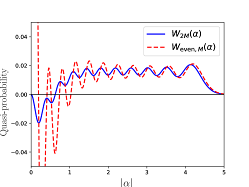
Figure 1. Colour online. Plots of the Wigner functions of $\rho_{2M}$ (solid line) and of $\rho_{\mathrm{even},M}$ (dashed line) as a function of $|\alpha|$ for $M=10$. Both states have comparable photon number: $\operatorname{Tr}(\rho_{2M}a^{\dagger}a)=M+\frac{1}{2}$, $\operatorname{Tr}(\rho_{\mathrm{even},M}a^{\dagger}a)=M+1$. The oscillations in the Wigner function of one are visibly much more pronounced than in the other, as detailed in the text.

5. Nonclassicality versus quantum macroscopicity

In contrast to the “nonclassicality” of a state, there is no generally agreed upon definition of its “quantum macroscopicity”, a property for which a variety of measures have been proposed recently [24, 25, 26, 28, 31, 33, 32, 34]. One such measure [33, 34] uses the quantum Fisher information $\mathcal{F}(\rho,Q_{\theta})$ of the quadratures $Q_{\theta}=Q\cos\theta+P\sin\theta$:

$${\mathcal{M}}_{\textrm{QFI}}(\rho)=\frac{1}{4}\max_{\theta}\mathcal{F}(\rho,Q_{\theta}).$$

We show in Appendix D that

$${\mathcal{M}}_{\textrm{QFI}}(\rho)>\frac{1}{2}\Rightarrow\rho\ \textrm{nonclassical},$$ (14)

proving that ${\mathcal{M}}_{\textrm{QFI}}$ is a nonclassicality witness, as ${S_{\mathrm{o}}}$: a large value of ${\mathcal{M}}_{\textrm{QFI}}$ guarantees the state is Glauber-Titulaer nonclassical. It is natural to ask how ${\mathcal{M}}_{\textrm{QFI}}$ and ${S_{\mathrm{o}}}$ are related. One may notice that on many states they behave similarly. Indeed, on thermal states and on $\rho_{M}$ (see the examples above), ${S_{\mathrm{o}}}=2{\mathcal{M}}_{\textrm{QFI}}$, so that they coincide except for a normalization (see Appendix D). The two can also be very different. For example, ${\mathcal{M}}_{\textrm{QFI}}$ is a less efficient nonclassicality witness than ${S_{\mathrm{o}}}$ for truncated vacuum states, while it is more efficient than ${S_{\mathrm{o}}}$ for squeezed thermal states. However, and more importantly, a large ${\mathcal{M}}_{\textrm{QFI}}$ does not imply a large ${\mathcal{N}}$, as the simple example $\rho_{k}=(1-\frac{M_{*}}{k})|0\rangle\langle 0|+\frac{M_{*}}{k}|k\rangle\langle k|$ shows: ${\mathcal{M}}_{\textrm{QFI}}(\rho_{k})=\frac{1}{2}+M_{*}$, ${\mathcal{N}}(\rho_{k})\to 0$ when $k\gg 1$. So, when $M_{*}$ is large, ${\mathcal{M}}_{\textrm{QFI}}$ is large, while the nonclassicality ${\mathcal{N}}$ remains small (see Appendix D for details). Consequently, if ${\mathcal{M}}_{\textrm{QFI}}$ does indeed correctly capture the idea of “quantum macroscopicity”, as proposed in [33, 34], then large quantum macroscopicity does not imply large nonclassicality in the sense of Glauber-Titulaer. This would seem to indicate that, even for a single mode, ${\mathcal{M}}_{\textrm{QFI}}$ captures “macroscopic” and/or “quantum” features of such states that are different from the nonclassicality associated with a nonpositive Sudarshan-Glauber $P$ function and revealed by their OS. What these features are, remains unclear. In all examples we treated, a large nonclassicality ${\mathcal{N}}$ implies a large ${\mathcal{M}}_{\textrm{QFI}}$, but whether this is generally true is not clear.

6. Conclusions

We have constructed a new measure ${\mathcal{N}}(\rho)$ for the nonclassicality of the states of a single-component boson field. ${\mathcal{N}}(\rho)$ is a distance to the set ${\mathcal{C}}$ of all classical states, defined in terms of the ordering sensitivity (OS) of the state, a new entropic notion that we introduced and that evaluates the sensitivity of the state to operator ordering. We have proven the crucial properties that all classical states have an OS less than one and that, when the OS of a density matrix is large, it provides a good approximation of ${\mathcal{N}}(\rho)$. The OS is easily computable in terms of field quadratures, captures several intuitive features of nonclassicality naturally, and detects in many cases nonclassicality more efficiently than previously known indicators. We have finally compared the nonclassicality ${\mathcal{N}}(\rho)$ to a recent proposal for the measure of “quantum macroscopicity” based on the Quantum Fisher Information.

We expect that the extension of the ideas developed here to multi-mode fields will help to clarify the relations between the Titulaer-Glauber nonclassicality and other manifestations of nonclassical behaviour such as entanglement. Finally, since the ordering sensitivity ${S_{\mathrm{o}}}(\rho)$ is defined in terms of the $s$-ordered entropy $H(s,\rho)$, it can be used to establish fundamental relations between quantum theory and thermodynamics [44].

Acknowledgments. This work was supported in part by the Labex CEMPI (ANR-11-LABX-0007-01) and by the Nord-Pas de Calais Regional Council and FEDER through the Contrat de Projets État-Région (CPER), and in part by the European Union’Äôs Horizon 2020 research and innovation programme under grant agreement No 665148 (QCUMbER).

Appendix A Proof of the bound (5) on the ordering sensitivity of classical states

We need to show that, if $\rho$ is a classical state, then $0\leq-(1-s)H^{\prime}(s,\rho)\leq 1,s<1$. We will use equation (2). If $\rho$ is classical, it is of the form $\rho=\int_{\mathbb{C}}|\alpha\rangle\langle\alpha|P(\alpha){\mathrm{d}}\alpha,$ where $P(\alpha){\mathrm{d}}\alpha$ is a probability measure. Hence, $W_{s}$ solves for $s<1$ a backward diffusion equation with initial condition $W_{1}{\mathrm{d}}\alpha=P{\mathrm{d}}\alpha$, so that, for $0\leq\tau=1-s$, $D=\frac{1}{4}$,

$$W_{1-\tau}(\alpha)=\int G_{\tau}(\alpha-\alpha^{\prime})P(\alpha^{\prime}){\mathrm{d}}\alpha^{\prime},\quad\text{with}\quad G_{\tau}(\alpha)=(2\pi D\tau)^{-1}\exp\left(-\frac{|\alpha|^{2}}{2D\tau}\right).$$

Next, recalling that $H(s)=-\ln(\pi\parallel W_{s}\parallel_{2}^{2})$, one sees from equation (2) that for $\tau>0$

$$-H^{\prime}(1-\tau)=\frac{-\frac{{\mathrm{d}}}{{\mathrm{d}}\tau}\parallel W_{1-\tau}\parallel_{2}^{2}}{\parallel W_{1-\tau}\parallel_{2}^{2}}=\frac{1}{4}\frac{\parallel\nabla W_{1-\tau}\parallel_{2}^{2}}{\parallel W_{1-\tau}\parallel_{2}^{2}}\geq 0.$$

Hence, proving equation (5) is equivalent to proving, for all $0<\tau$,

$$\Lambda(\tau):=-\partial_{\tau}\parallel W_{1-\tau}\parallel_{2}^{2}-\frac{1}{\tau}\parallel W_{1-\tau}\parallel_{2}^{2}\leq 0.$$

Then

$$0\leq-\partial_{\tau}\|W_{1-\tau}\|^{2} = -2\int W_{1-\tau}(\alpha)\partial_{\tau}W_{1-\tau}(\alpha){\mathrm{d}}\alpha,$$

$$= -2\int\int W_{1-\tau}(\alpha)\left(-\frac{1}{\tau}+\frac{|\alpha-\alpha_{2}|^{2}}{2D\tau^{2}}\right)G_{\tau}(\alpha-\alpha_{2})W_{1}(\alpha_{2}){\mathrm{d}}\alpha{\mathrm{d}}\alpha_{2}$$

$$= 2\int\int W_{1}(\alpha_{1})G_{\tau}(\alpha-\alpha_{1})\tilde{G}_{\tau}(\alpha-\alpha_{2})W_{1}(\alpha_{2}){\mathrm{d}}\alpha{\mathrm{d}}\alpha_{1}{\mathrm{d}}\alpha_{2},$$

where $\tilde{G}_{\tau}(\alpha)=-\left(-\frac{1}{\tau}+\frac{|\alpha|^{2}}{2D\tau^{2}}\right)G_{\tau}(\alpha).$ So

$$\Lambda(\tau)=\int W_{1}(\alpha_{1})S_{\tau}(\alpha_{1},\alpha_{2})W_{1}(\alpha_{2}){\mathrm{d}}\alpha_{1}{\mathrm{d}}\alpha_{2}$$

with

$$S_{\tau}(\alpha_{1},\alpha_{2})=\int G_{\tau}(\alpha-\alpha_{1})\left[\frac{2}{\tau}-\frac{1}{\tau}-\frac{2|\alpha-\alpha_{1}|^{2}}{2D\tau^{2}}\right]G_{\tau}(\alpha-\alpha_{2}){\mathrm{d}}\alpha.$$

Integrating over $\alpha$ in this expression, one finds

$$S_{\tau}(\alpha_{1},\alpha_{2})=\frac{1}{4\pi D\tau}\exp(-\frac{|\alpha_{1}-\alpha_{2}|^{2}}{4D\tau})\left[-\frac{|\alpha_{1}-\alpha_{2}|^{2}}{4D\tau^{2}}\right].$$

This expression is negative, so it follows from the positivity of $W_{1}(\alpha){\mathrm{d}}\alpha$ for all $\alpha$ that $\Lambda(\tau)\leq 0$, which is the desired result. Note that $\Lambda(\tau)=0$ if and only if $W_{1}(\alpha){\mathrm{d}}\alpha$ is a Dirac delta measure, which corresponds to a coherent state.

Remarks. (a) In the presence of $d$ modes, the same computation as above yields

$$0\leq-(1-s)H^{\prime}(s,\rho)\leq\frac{d}{2},\quad s<1.$$

The theory can therefore be adapted to multi-component bose fields. (b) We point out the following subtlety. That $P(\alpha){\mathrm{d}}\alpha$ is a probability measure does not imply $P$ is square integrable: $\int P^{2}(\alpha){\mathrm{d}}\alpha$ may be infinity, such as when $P(\alpha)=\delta(\alpha-\alpha_{0})$. However, the Young inequality for convolutions [45] guarantees that $W_{s}$ for $s<1$ is square integrable. This is not true for all states, but it is for classical states and legitimizes the computations of the $L^{2}$-norms above.

Appendix B Ordering sensitivity as a Hilbert space norm

We first show (10). An easy computation shows that, if $W_{A}$ is the Wigner function of an operator $A$, then $\partial_{\alpha_{1}}W_{A}$ is the Wigner function of $\sqrt{2}i[A,P]$ and $\partial_{\alpha_{2}}W_{A}$ of $\sqrt{2}i[A,Q]$. It follows then from (9) that

$$\langle A,B\rangle=\frac{\pi}{4}\int\overline{\nabla W_{A}(\alpha)}\nabla W_{B}(\alpha){\mathrm{d}}\alpha.$$ (15)

Taking $A=B=\rho$, one finds (10) . Note that what precedes is formal, since, as a result of the fact that $Q$ and $P$ are unbounded operators, ${\left|\kern-1.07639pt\left|\kern-1.07639pt\left|A\right|\kern-1.07639pt\right|\kern-1.07639pt\right|}$ can be equal to $+\infty$, and the inner product $\langle A,B\rangle$ may be ill defined. To avoid this problem, we proceed as follows. We write ${\mathcal{L}}_{\textrm{HS}}$ for the set of Hilbert-Schmidt operators, i.e. those operators $A$ for which $\operatorname{Tr}(A^{\dagger}A)<+\infty$. We then define the following vector space of operators:

$${\mathcal{L}}_{\textrm{HS}}^{(1)}=\{A\in{\mathcal{L}}_{\textrm{HS}}\mid[A,Q],[A,P]\in{\mathcal{L}}_{\textrm{HS}}\}.$$

On it, $\langle A,B\rangle$ is always finite and defines a sesquilinear form, linear in $B$ and anti-linear in $A$. To see the above mathematical precautions are necessary, consider a pure state $\rho=|\psi\rangle\langle\psi|$. Then $\operatorname{Tr}[\rho,Q]^{2}=-2\Delta Q^{2},\operatorname{Tr}[\rho,P]^{2}=-2\Delta P^{2}.$ These traces are finite if and only if $\langle\psi|(Q^{2}+P^{2})|\psi\rangle=2\langle\psi|a^{\dagger}a|\psi\rangle+1$ is finite. In other words, if and only if the mean photon number of the state $|\psi\rangle$ is finite. This is not a very restrictive condition, but it is essential, and it is satisfied by all states commonly considered in the literature. We remark that, similarly, the right hand side of (15) is in general not finite for arbitrary operators $A$ and $B$, even if they are both trace class. Indeed, whereas then the Wigner function is square integrable, nothing guarantees its gradient is as well. Whence the need to restrict to the space ${\mathcal{L}}_{\textrm{HS}}^{(1)}$ for which this is the case: assuming $[\rho,Q]$, respectively $[\rho,P]$, are trace class implies indeed $\partial_{\alpha_{2}}W$, respectively $\partial_{\alpha_{1}}W$ are square integrable. We now show that the above sesquilinear form is non-degenerate, in the sense that ${\left|\kern-1.07639pt\left|\kern-1.07639pt\left|A\right|\kern-1.07639pt\right|\kern-1.07639pt\right|}=0$ implies $A=0$. As a result, it is an inner product and ${\mathcal{L}}_{\textrm{HS}}^{(1)}$ is a pre-Hilbert space. With the usual abuse of notation, we will write ${\mathcal{L}}_{\textrm{HS}}^{(1)}$ for its completion as a Hilbert space as well. We give two proofs. First note that ${\left|\kern-1.07639pt\left|\kern-1.07639pt\left|A\right|\kern-1.07639pt\right|\kern-1.07639pt\right|}=0$ implies $[A,Q]=0=[A,P]$. Since the Weyl-Heisenberg group acts irreducibly, an operator that commutes with both $Q$ and $P$ must be a multiple of the identity. Since $A$ is trace class, this implies $A=0$. Alternatively, take $A=B$ in (15), note that $\langle A,A\rangle=0$ implies $\nabla W_{A}=0$. Hence $W_{A}$ is a constant. Since $\int|W_{A}|^{2}(\alpha){\mathrm{d}}\alpha<+\infty$, $W_{A}=0$ and hence $A=0$.

Note that the right hand side of (15) defines an inner product on the space of functions of $\alpha\in\mathbb{C}$. It is well known as a homogeneous Sobolev inner product [46] and the space of functions for which $\|\nabla W\|$ is finite is the homogeneous Sobolev space denoted by $\dot{H}^{1,2}(\mathbb{C})$, important in the study of partial differential equations. One can therefore think of ${\mathcal{L}}_{\textrm{HS}}^{(1)}$ as a quantum or non-commutative Sobolev space.

We now show (13). We have

$$\operatorname{Tr}[\rho,Q][Q,\rho]=\sum_{i}p_{i}^{2}\operatorname{Tr}\left[|i\rangle\langle i|,Q\right]\left[Q,|i\rangle\langle i|\right]+\sum_{i\not=j}p_{i}p_{j}\operatorname{Tr}[|i\rangle\langle i|,Q][Q,|j\rangle\langle j|].$$

Since $\operatorname{Tr}\left[|i\rangle\langle i|,Q\right]\left[Q,|i\rangle\langle i|\right]=2\Delta Q_{i}^{2}$ and, for $i\not=j$,

$$\operatorname{Tr}[|i\rangle\langle i|,Q][Q,|j\rangle\langle j|]=-2|\langle i|Q|j\rangle|^{2},$$

the result follows.

Continuity is a desirable property for any non-classicality measure [23]: small changes in the state should lead to small changes in its non-classicality. Since the ordering sensitivity is a norm, it is automatically continuous and so is therefore the induced distance to the set $\tilde{\mathcal{C}}$.

We finally establish some simple geometric properties of $\tilde{\mathcal{C}}$ helping to locate it more precisely within the unit ball of ${\mathcal{L}}_{\textrm{HS}}^{(1)}$, and that will allow us to prove (12). We have seen that $\tilde{\rho}\in\tilde{\mathcal{C}}$ satisfies ${\left|\kern-1.07639pt\left|\kern-1.07639pt\left|\tilde{\rho}\right|\kern-1.07639pt\right|\kern-1.07639pt\right|}=1$ iff and only if $\rho$ is a coherent state, and hence a pure state. So the pure classical states all lie on the unit sphere of ${\mathcal{L}}_{\textrm{HS}}^{(1)}$. It is natural to wonder how far the $\tilde{\rho}\in\tilde{\mathcal{C}}$, which lie inside the unit ball, can be removed from its surface, the unit sphere. In that perspective, we point out that, using (13) with the Fock basis, one easily sees that for a thermal state $\rho_{\mathrm{th}}$ with mean photon number $\langle n\rangle$, ${S_{\mathrm{o}}}(\rho_{\mathrm{th}})=(2\langle n\rangle+1)^{-1}.$ Hence, as $\langle n\rangle\to+\infty$, ${S_{\mathrm{o}}}(\rho_{\mathrm{th}})={\left|\kern-1.07639pt\left|\kern-1.07639pt\left|\tilde{\rho}_{\mathrm{th}}\right|\kern-1.07639pt\right|\kern-1.07639pt\right|}\to 0$. Hence the set $\tilde{\mathcal{C}}$ contains elements arbitrarily close to the center of the unit ball, far from the surface of the sphere of radius one. It is tempting to think of such states as very classical. Since large photon number corresponds to high temperature, this is in agreement again with basic physical intuition. We can now show (12). The lower bound is obvious. By the definition of ${\mathcal{N}}(\rho)$ and the triangle inequality for norms we have ${\mathcal{N}}(\rho)\leq{\left|\kern-1.07639pt\left|\kern-1.07639pt\left|\tilde{\rho}-\tilde{\rho}_{\mathrm{th}}\right|\kern-1.07639pt\right|\kern-1.07639pt\right|}\leq{\left|\kern-1.07639pt\left|\kern-1.07639pt\left|\tilde{\rho}\right|\kern-1.07639pt\right|\kern-1.07639pt\right|}+{\left|\kern-1.07639pt\left|\kern-1.07639pt\left|\tilde{\rho}_{\mathrm{th}}\right|\kern-1.07639pt\right|\kern-1.07639pt\right|}.$ Taking $\langle n\rangle$ to infinity, we find ${\mathcal{N}}(\rho)\leq{\left|\kern-1.07639pt\left|\kern-1.07639pt\left|\tilde{\rho}\right|\kern-1.07639pt\right|\kern-1.07639pt\right|}.$

Appendix C On the non-classicality of multi-component cat states

Multi-component cat states [42, 43] are superpositions of $N$ coherent states placed at the points $\alpha_{m}=\alpha_{0}\exp(-i\frac{2\pi}{N}m)$:

$$|\mathrm{c}_{q}\rangle=\frac{1}{N\sqrt{\tilde{g}(q)}}\sum_{m=0}^{N-1}e^{i2\pi mq/N}|\alpha_{0}e^{-i2\pi m/N}\rangle,\quad\tilde{g}(q)=\frac{1}{N}\sum_{m=0}^{N-1}g(m)e^{-i2\pi qm/N},$$

with

$$g(m)=\exp\left\{|\alpha_{0}|^{2}\left(e^{i2\pi m/N}-1\right)\right\}.$$

All expressions only depend on the integer $q$ modulo $N\geq 2$ and $\langle c_{q}|c_{q^{\prime}}\rangle=\delta_{q,q^{\prime}\text{mod}N}$; $N=2$ yields even/odd ($q=0,1$) cat states. We first establish that the ordering sensitivity of these states tends to infinity with $\alpha_{0}$ at fixed $N$ proving their strong non-classicality. We will then show that neither the Mandel parameter $Q_{\textrm{M}}$, nor the degree of squeezing $S$, defined below, nor the moment method [7] detect the non-classicality of the $N$ component cat states for large $|\alpha_{0}|$.

We have, for all $\ell\in{\mathbb{Z}}$:

$$a^{\ell}|c_{q}\rangle=\alpha_{0}^{\ell}\sqrt{\frac{\tilde{g}(q-\ell)}{\tilde{g}(q)}}|c_{q-\ell}\rangle,\quad\langle c_{q}|(a^{\dagger})^{\ell}a^{\ell}|c_{q}\rangle=\frac{\tilde{g}(q-\ell)}{\tilde{g}(q)}|\alpha_{0}|^{2\ell}.$$ (16)

Hence ${S_{\mathrm{o}}}(N,q)=2\frac{\tilde{g}(q-1)}{\tilde{g}(q)}|\alpha_{0}|^{2}+1$ which tends to infinity with growing $|\alpha_{0}|$, proving the first assertion. We now turn to the moment method. It is shown in [7] that a sufficient condition for the non-classicality of a state $\rho$ is the negativity of one of the following determinants:

$$D_{n}=\left|\begin{matrix}1&m_{1}&\dots&m_{n-1}\\ m_{1}&m_{2}&\dots&m_{n}\\ \vdots&\vdots&\vdots&\vdots\\ m_{n-1}&m_{n}&\dots&m_{2n-2}\end{matrix}\right|,\quad\textrm{where}\quad m_{\ell}=\operatorname{Tr}\rho(a^{\dagger})^{\ell}a^{\ell}.$$

Note that $D_{2}=Q_{\textrm{M}}$, the Mandel parameter.

In general, the computation of the $D_{n}$ becomes increasingly complex with growing $n$, since it requires the computation or measurement of higher order moments $m_{\ell}$. Here, using (16) one finds, for general $\alpha_{0},N,q,n$,

$$D_{n}(q)=\frac{|\alpha_{0}|^{2n(n-1)}}{\tilde{g}(q)^{n}}\textrm{det}\,\tilde{G}(q),$$

where

$$\tilde{G}(q)=\begin{pmatrix}{\tilde{g}(q)}&{\tilde{g}(q-1)}&\dots&{\tilde{g}(q-(n-1))}\\ {\tilde{g}(q-1)}&{\tilde{g}(q-2)}&\dots&{\tilde{g}(q-(n-1)-1)}\\ \vdots&\vdots&\vdots&\vdots\\ {\tilde{g}(q-(n-1))}&{\tilde{g}(q-(n-1)-1)}&\dots&{\tilde{g}(q-2(n-1))}\end{pmatrix}.$$ (17)

Because of the $N$-periodicity of $\tilde{g}$, $D_{n}(q)=0$ for $n>N$. To compute $D_{n}$, we compute, for $m\not=0$ mod $N$,

$$|g(m)|=\exp\left(|\alpha_{0}|^{2}(\cos(\frac{2\pi m}{N})-1)\right)\leq\exp\left(-\frac{|\alpha_{0}|^{2}}{2}\eta\left(\frac{2\pi}{N}\right)^{2}\right),$$

with $\eta=1-\frac{1}{12}\left(\frac{2\pi}{N}\right)^{2}$, since, for all $x\in\mathbb{R}$, $\cos(x)-1+\frac{x^{2}}{2}\leq\frac{x^{4}}{24}.$ Hence

$$\tilde{g}(q)=\frac{1}{N}+r(q),\quad\textrm{with}\quad|r(q)|\leq\overline{r}=\frac{N-1}{N}\exp\left(-\frac{|\alpha_{0}|^{2}}{2}\eta\left(\frac{2\pi}{N}\right)^{2}\right).$$

Note that the estimate on the error term $r(q)$ does not depend on $q$. Introducing $\underline{e}=N^{-1/2}(1,1,\dots,1)$, we have

$$D_{n}=\frac{|\alpha_{0}|^{2n(n-1)}}{\tilde{g}(q)^{n}}\textrm{det}\left(\underline{e}^{T}\underline{e}+R(q)\right),$$

where $R(q)$ is obtained from $r(q)$ in the same manner as $\tilde{G}(q)$ from $\tilde{g}(q)$ in (17). It follows from the matrix determinant lemma that $\textrm{det}(R(q)+\underline{e}^{T}\underline{e})=\textrm{det}R(q)+\underline{e}\textrm{adj}R(q)\underline{e}^{T},$ where adj$R(q)$ is the adjugate matrix of $R(q)$, meaning the transpose of the matrix of its cofactors. Hence

$$|D_{n}|=\frac{|\alpha_{0}|^{2n(n-1)}}{\tilde{g}(q)^{n}}\left|\textrm{det}R(q)+\underline{e}\textrm{adj}R(q)\underline{e}^{T}\right|\leq\frac{|\alpha_{0}|^{2n(n-1)}}{\tilde{g}(q)^{n}}n!\overline{r}^{(n-1)}\left[\overline{r}+\frac{n}{N}\right].$$

Therefore, for fixed $N,n,q$, the determinant $D_{n}$ tends very quickly to zero with growing $\alpha_{0}$. Its negativity is therefore increasingly difficult to observe. In this sense, the moment method does not efficiently detect the growing non-classicality of the multi component cat states for growing $\alpha_{0}$. In addition, observing $D_{2}$ closely as a function of $\alpha_{0}$, one observes it oscillates around zero, changing sign regularly as $\alpha_{0}$ grows.

For the degree of squeezing S [7], defined for each $\varphi\in[0,2\pi[$ by

$$S=\langle:(a\exp(i\varphi)+a^{\dagger}\exp(-i\varphi))^{2}:\rangle-\langle(a\exp(i\varphi)+a^{\dagger}\exp(-i\varphi))\rangle^{2}$$

we find, since $\langle a\rangle=0$, $S=\langle a^{2}\exp(2i\varphi)+(a^{\dagger})^{2}\exp(-2i\varphi)+2a^{\dagger}a\rangle.$ Now $a^{2}|c_{q}\rangle=\alpha_{0}^{2}\sqrt{\tilde{g}(q-2)\tilde{g}(q)^{-1}}|c_{q-2}\rangle.$ Hence, if $N\geq 3$, $\langle a^{2}\rangle=0$. One has then $S=2\langle c_{q}|a^{\dagger}a|c_{q}\rangle=2\frac{\tilde{g}(q-1)}{\tilde{g}(q)}|\alpha_{0}|^{2}>0.$ Since negativity of $S$ is a witness of non-classicality, one concludes that the non-classicality of the multi component cat states is not detected by the degree of squeezing if $N\geq 3$. The case $N=2$ is slightly different. Then $a^{2}|c_{q}\rangle=\alpha_{0}^{2}|c_{q}\rangle$ and, for $q=0,1$

$$S(2,q)=2\alpha_{0}^{2}\left(\cos(2\varphi)+\frac{\tilde{g}(q-1)}{\tilde{g}(q)}\right),\quad\tilde{g}(1)=1-\langle\alpha|-\alpha\rangle,\quad\tilde{g}(0)=1+\langle\alpha|-\alpha\rangle.$$

So the even cat shows squeezing, the odd one does not.

Appendix D Nonclassicality versus quantum macroscopicity

The Quantum Fisher Information (QFI) $\mathcal{F}(\rho,A)$ of the state $\rho$ for the observable $A$ is defined as [47]

$$\mathcal{F}(\rho,A)=4\partial_{x}^{2}D_{B}^{2}(\rho,\exp(-ixA)\rho\exp(ixA)_{|x=0},$$

where $D_{B}^{2}(\rho,\sigma)=2(1-F(\rho,\sigma))$ is the Bures distance and $F(\rho,\sigma)=\operatorname{Tr}\sqrt{\sqrt{\rho}\sigma\sqrt{\rho}}$ the fidelity between $\rho$ and $\sigma$. Explicitly,

$$\mathcal{F}(\rho,A)=2\sum_{i,j}\frac{(p_{i}-p_{j})^{2}}{p_{i}+p_{j}}|\langle i|A|j\rangle|^{2}=4\sum_{i<j}\frac{(p_{i}-p_{j})^{2}}{p_{i}+p_{j}}|\langle i|A|j\rangle|^{2},$$ (18)

where $\rho=\sum_{i}p_{i}|i\rangle\langle i|$ is a spectral decomposition of $\rho$ and the sum is over $i,j$ for which $p_{i}+p_{j}>0$. It was proven in [29, 30] that the QFI is equal to the convex roof of four times the variance of $A$ seen as a function on pure states. As pointed out in Section 5, the authors of [33, 34] propose a measure ${\mathcal{M}}_{\textrm{QFI}}(\rho)$ of quantum macroscopicity for the state $\rho$ of a bosonic field using the Fisher information as follows:

$${\mathcal{M}}_{\textrm{QFI}}(\rho)=\frac{1}{4}\sup_{\theta}\mathcal{F}(\rho,Q_{\theta}),\quad Q_{\theta}=\cos\theta Q+\sin\theta P.$$

We now show equation (14). Since $\mathcal{F}(\rho,Q_{\theta})$ is convex, and for a coherent state, $\Delta Q_{\theta}^{2}=\frac{1}{2}$, one has, for any classical $\rho=\int P(\alpha)|\alpha\rangle\langle\alpha|{\mathrm{d}}\alpha,$

$${\mathcal{M}}_{\textrm{QFI}}(\rho)\leq\int P(\alpha)\frac{1}{4}\mathcal{F}(|\alpha\rangle\langle\alpha|,Q_{\theta}){\mathrm{d}}\alpha=\frac{1}{2}.$$

Consequently, if ${\mathcal{M}}_{\textrm{QFI}}(\rho)>\frac{1}{2}$, then $\rho$ is nonclassical, proving the claim that ${\mathcal{M}}_{\textrm{QFI}}$ is a nonclassicality witness.

To further explore the relation between ${S_{\mathrm{o}}}$ and ${\mathcal{M}}_{\textrm{QFI}}$, we compute ${\mathcal{M}}_{\textrm{QFI}}$ for the various benchmark states studied in the main part of the paper. If $\rho$ is of the form $\rho=\sum_{n}p_{n}|n\rangle\langle n|$, where the $|n\rangle$ are the Fock states then

$$\mathcal{F}(\rho,Q_{\theta})=4\sum_{n<m}\frac{(p_{n}-p_{m})^{2}}{p_{n}+p_{m}}|\langle n|Q|m\rangle|^{2}=2\sum_{n}\frac{(p_{n}-p_{n+1})^{2}}{p_{n}+p_{n+1}}(n+1)$$

and

$$\frac{1}{2}\operatorname{Tr}[\rho,Q][Q,\rho] = \frac{1}{2}\operatorname{Tr}[\rho,P][P,\rho]=\sum_{n<m}(p_{n}-p_{m})^{2}|\langle n|Q|m\rangle|^{2}$$

$$= \frac{1}{2}\sum_{n}(p_{n}-p_{n+1})^{2}(n+1).$$

First, consider states $\rho_{N,M}$, with $p_{n}=M^{-1}$ for all $N+1\leq n\leq N+M$ and $p_{n}=0$ otherwise, for some $N\geq 0,M>0$, two integers. Then

$$S_{0}(\rho)=1+2\frac{N+1}{M}>1,\quad{\mathcal{M}}_{\textrm{QFI}}(\rho)=\frac{1}{4}\mathcal{F}(\rho,Q)=\frac{1}{2}+\frac{N+1}{M}>\frac{1}{2}$$

so that ${\mathcal{M}}_{\textrm{QFI}}(\rho)=\frac{1}{2}{S_{\mathrm{o}}}(\rho).$ So, for these states, the ordering sensitivity introduced here and the quantum macroscopicity measure of [33, 34] coincide up to a global normalization. Note that these states are non-classical and both quantities detect this. Their Mandel parameter, on the other hand, one finds

$$Q_{\textrm{M}}=(\frac{1}{12}M(M-6)-\frac{7}{12}-N)\langle a^{\dagger}a\rangle^{-1},\quad\langle a^{\dagger}a\rangle=\frac{1}{2}(M+1)+N.$$

This is positive for $M$ sufficiently large and therefore does not detect their nonclassicality.

For thermal states $\rho_{\textrm{th}}$, where $p_{n}=\mathcal{N}_{\lambda}\exp(-\lambda n)$ one has similarly

$$S_{0}(\rho_{\textrm{th}})=\operatorname{Tr}\rho_{\textrm{th}}^{2}=\frac{1}{2}\mathcal{F}(\rho_{\textrm{th}},Q)=2{\mathcal{M}}_{\textrm{QFI}}(\rho_{\textrm{th}}).$$

Note that, since the thermal states are classical, one has indeed ${S_{\mathrm{o}}}(\rho_{\textrm{th}})<1$.

For the Truncated Thermal States introduced in [8], given by $\rho_{\textrm{TTS}}=(\exp(\beta)-1)\sum_{n=1}^{+\infty}\exp(-\beta n)|n\rangle\langle n|,$ one has $Q_{\textrm{M}}(\rho_{\textrm{TTS}})=(\exp(\beta)-1)^{-1}-1=\langle\hat{n}\rangle_{\beta}-2,$ and

$${S_{\mathrm{o}}}(\rho_{\textrm{TTS}})=(1-{\mathrm{e}}^{-\beta})\left(2+\frac{1}{1+{\mathrm{e}}^{-\beta}}\right),\quad{\mathcal{M}}_{\textrm{QFI}}(\rho_{\textrm{TTS}})=\frac{3}{2}\frac{1-{\mathrm{e}}^{-\beta}}{1+{\mathrm{e}}^{-\beta}}.$$

It follows the nonclassicality of these states is detected by $Q_{\textrm{M}}$ and by ${\mathcal{M}}_{\textrm{QFI}}$ provided $\beta>\ln 2\simeq 0.6931$ and by ${S_{\mathrm{o}}}$ for $\beta>\ln\frac{2}{\sqrt{5}-1}\simeq 0.4812$. Consequently, the ordering sensitivity outperforms the two other witnesses for these states.

In the previous families of examples, when there are differences between the behaviour of the nonclassicality measure ${\mathcal{N}}$ and the quantum macroscopicity measure ${\mathcal{M}}_{\textrm{QFI}}$, they occur at low levels of nonclassicality, whereas the asymptotically large values tend to agree. We now give a simple example where the two differ considerably for large values. For that purpose, let us consider $\rho_{k}=(1-\epsilon_{k})|0\rangle\langle 0|+\epsilon_{k}|k\rangle\langle k|.$ Then

$${S_{\mathrm{o}}}(\rho_{k})=1+2\frac{k\epsilon_{k}^{2}}{(1-\epsilon_{k})^{2}+\epsilon_{k}^{2}}\quad\textrm{and}\quad{\mathcal{M}}_{\textrm{QFI}}(\rho)=\frac{1}{2}+k\epsilon_{k}.$$

Taking $\epsilon_{k}=M_{*}k^{-1}$, one has ${\mathcal{M}}_{\textrm{QFI}}(\rho_{k})=\frac{1}{2}+M_{*}$ and ${S_{\mathrm{o}}}(\rho_{k})\to 1$ as $k\to+\infty$. In fact ${\mathcal{N}}(\rho_{k})\leq|||\tilde{\rho}_{k}-|0\rangle\langle 0||||\to 0.$ This example shows that ${\mathcal{M}}_{\textrm{QFI}}$ can be arbitrarily large, while the nonclassicality ${\mathcal{N}}$ is arbitrarily small. This means that, whereas ${\mathcal{M}}_{\textrm{QFI}}$ can act as a nonclassicality witness, it cannot serve as a nonclassicality measure. Consequently, whenever one finds a state with a large value of the quantum macroscopicity measure ${\mathcal{M}}_{\textrm{QFI}}$, one cannot conclude it has a large nonclassicality or ordering sensitivity. In the last example, the large value of ${\mathcal{M}}_{\textrm{QFI}}$ must be attributed to another property of the state than its ordering sensitivity.

As a final example, we consider squeezed thermal states. Those are defined as $\rho_{\textrm{sqth}}=S(z)\rho_{\textrm{th}}S(z)^{\dagger},$ where $z=r\exp(i\varphi)$ is the squeezing parameter and $S(z)=\exp\left\{\frac{z^{*}}{2}a^{2}-\frac{z}{2}a^{\dagger 2}\right\}$. Note that they are not rotationally invariant. Their eigenstates are $S(z)|n\rangle$ and using (18), one finds $\mathcal{F}(\rho_{\textrm{sqth}},Q_{\theta})=|C_{\theta}|^{2}\frac{2}{2\langle n\rangle_{\textrm{th}}+1}$ where $C_{\theta}=\cosh r-\exp(2i\theta-i\varphi)\sinh r$. Hence ${\mathcal{M}}_{\textrm{QFI}}(\rho_{\textrm{sqth}})={\mathcal{M}}_{\textrm{QFI}}(\rho_{\textrm{th}})\exp(2r)=\frac{1}{2}\frac{1}{2\langle n\rangle_{\textrm{th}}+1}\exp(2r).$ It follows that ${\mathcal{M}}_{\textrm{QFI}}(\rho_{\textrm{sqth}})>1/2$ iff $r>\frac{1}{2}\ln(2\langle n\rangle_{\textrm{th}}+1)$. It is known [48] that this condition is necessary and sufficient for the nonclassicality of squeezed thermal states so that ${\mathcal{M}}_{\textrm{QFI}}$ detects this property optimally for those states. For ${S_{\mathrm{o}}}$, one finds, on the other hand ${S_{\mathrm{o}}}(\rho_{\textrm{sqth}})=\frac{1}{2\langle n\rangle_{\textrm{th}}+1}\cosh(2r).$ The condition ${S_{\mathrm{o}}}(\rho_{\textrm{sqth}})>1$ yields a condition on $r$ for nonclassicality, which is however suboptimal in this case. So for this example, the quantum macroscopicity ${\mathcal{M}}_{\textrm{QFI}}$ is a better nonclassicality witness than the ordering sensitivity ${S_{\mathrm{o}}}$. Note however this. From (12), we see that, asymptotically for large $r$, ${\mathcal{N}}(\rho_{\textrm{sqth}})\sim\exp(r)$: the squeezed thermal states are exponentially far from classical in the squeezing parameter $r$. From the large value of ${\mathcal{M}}_{\textrm{QFI}}$, such information cannot be inferred a priori, as the previous example shows.

References

- [1] U. M. Titulaer and R. J. Glauber. Correlation functions for coherent fields. Phys. Rev., 140:B676–B682, Nov 1965.
- [2] M. Hillery. Classical pure states are coherent states. Phys. Lett., 111 A:409, 1985.
- [3] A. Bach and U. Lüxmann-Ellinghaus. The simplex structure of the classical states of the quantum harmonic oscillator. Commun.Math. Phys., 107:553, 1986.
- [4] Mark Hillery. Nonclassical distance in quantum optics. Phys. Rev. A, 35:725–732, Jan 1987.
- [5] Mark Hillery. Total noise and nonclassical states. Phys. Rev. A, 39:2994–3002, Mar 1989.
- [6] Ching Tsung Lee. Measure of the nonclassicality of nonclassical states. Phys. Rev. A, 44:R2775–R2778, Sep 1991.
- [7] G. S. Agarwal and K. Tara. Nonclassical character of states exhibiting no squeezing or sub-poissonian statistics. Phys. Rev. A, 46:485–488, Jul 1992.
- [8] Ching Tsung Lee. Theorem on nonclassical states. Phys. Rev. A, 52:3374–3376, Oct 1995.
- [9] N. Lütkenhaus and Stephen M. Barnett. Nonclassical effects in phase space. Phys. Rev. A, 51:3340–3342, Apr 1995.
- [10] V.V. Dodonov, O.V. Man’ko, A. O. Man’ko, and A. Wünsche. Hilbert-schmidt distance and non-classicality of states in quantum optics. J. Mod. Opt., 47:633, 2000.
- [11] Paulina Marian, Tudor A. Marian, and Horia Scutaru. Quantifying nonclassicality of one-mode gaussian states of the radiation field. Phys. Rev. Lett., 88:153601, Mar 2002.
- [12] Th. Richter and W. Vogel. Nonclassicality of quantum states: A hierarchy of observable conditions. Phys. Rev. Lett., 89:283601, Dec 2002.
- [13] A. Kenfack and K. Zyczkowski. Negativity of the wigner function as an indicator of non-classicality. J. Opt. B: Quantum Semiclass. Opt., 6:396, 2004.
- [14] János K. Asbóth, John Calsamiglia, and Helmut Ritsch. Computable measure of nonclassicality for light. Phys. Rev. Lett., 94:173602, May 2005.
- [15] A. A. Semenov, D.Yu. Vasylyev, and B. I. Lev. non-classicality of noisy quantum states. J. Phys. B: At. Mol. Opt. Phys., 39:905–916, 2006.
- [16] Alessandro Zavatta, Valentina Parigi, and Marco Bellini. Experimental nonclassicality of single-photon-added thermal light states. Phys. Rev. A, 75:052106, May 2007.
- [17] W. Vogel and J. Sperling. Unified quantification of nonclassicality and entanglement. Phys. Rev. A, 89:052302, May 2014.
- [18] S. Ryl, J. Sperling, E. Agudelo, M. Mraz, S. Köhnke, B. Hage, and W. Vogel. Unified nonclassicality criteria. Phys. Rev. A, 92:011801, Jul 2015.
- [19] J. Sperling and W. Vogel. Convex ordering and quantification of quantumness. Phys. Scr., 90:074024, 2015.
- [20] N. Killoran, F. E. S. Steinhoff, and M. B. Plenio. Converting nonclassicality into entanglement. Phys. Rev. Lett., 116:080402, Feb 2016.
- [21] M. Alexanian. Non-classicality criteria: Glauber-sudarshan p function and mandel parameter. Journal of Modern Optics, 2017.
- [22] Ranjith Nair. Nonclassical distance in multimode bosonic systems. Phys. Rev. A, 95:063835, Jun 2017.
- [23] S. Ryl, J. Sperling, and W. Vogel. Quantifying nonclassicality by characteristic functions. Phys. Rev. A, 95:053825, May 2017.
- [24] A J Leggett. Testing the limits of quantum mechanics: motivation, state of play, prospects. Journal of Physics: Condensed Matter, 14(15):R415, 2002.
- [25] Chang-Woo Lee and Hyunseok Jeong. Quantification of macroscopic quantum superpositions within phase space. Phys. Rev. Lett., 106:220401, May 2011.
- [26] J. Gong. Comment on “quantification of macroscopic quantum superpositions within phase space”. arXiv:1106.0062v2, 2011.
- [27] Chang-Woo Lee and Hyunseok Jeong. Quantification of macroscopic quantum superpositions within phase space. arXiv:1108.0212v1, 2011.
- [28] F. Fröwis and W. Dür. Measures of macroscopicity for quantum spin systems. New Journal of Physics, 14:093039, 2012.
- [29] Géza Tóth and Dénes Petz. Extremal properties of the variance and the quantum fisher information. Phys. Rev. A, 87:032324, Mar 2013.
- [30] S. Yu. arXiv:1302.5311, 2013.
- [31] Pavel Sekatski, Nicolas Gisin, and Nicolas Sangouard. How difficult is it to prove the quantumness of macroscropic states? Phys. Rev. Lett., 113:090403, Aug 2014.
- [32] F. Fröwis, N. Sangouard, and N. Gisin. Linking measures for macroscopic quantum states via photon-spin mapping. Optics Communications, 337, 2015.
- [33] E. Oudot, P. Sekatski, P. Fröwis, N. Gisin, and N. Sangouard. Two-mode squeezed states as schr?dinger cat-like states. Journal of the Optical Society of America B, 32:2190, 2015.
- [34] Benjamin Yadin and Vlatko Vedral. General framework for quantum macroscopicity in terms of coherence. Phys. Rev. A, 93:022122, Feb 2016.
- [35] Borivoje Dakić and Milan Radonjić. Macroscopic superpositions as quantum ground states. Phys. Rev. Lett., 119:090401, Sep 2017.
- [36] Y. Gu. Evidences of classical and quantum chaos in the time evolution of nonequilibrium ensembles. Phys. Lett., 149:95, 1990.
- [37] Jiangbin Gong and Paul Brumer. Chaos and quantum-classical correspondence via phase-space distribution functions. Phys. Rev. A, 68:062103, Dec 2003.
- [38] K. Cahill and R. J. Glauber. Density operators and quasi-probability distributions. Phys. Rev., 177:1882, 1969.
- [39] G.B. Folland. Analysis on phase space. Princeton University Press, 1989.
- [40] L. Mandel and E. Wolf. Optical coherence and quantum optics. Cambridge University Press, 1995.
- [41] K. Cahill and R. J. Glauber. Ordered expansions in boson amplitude operators. Phys. Rev., 177:1857, 1969.
- [42] S. Haroche and J. M. Raimond. Exploring the Quantum: Atoms, Cavities, and Photons. Oxford Graduate Texts, 2013.
- [43] D. B. Horoshko, S. De Bièvre, M. I. Kolobov, and G. Patera. Entanglement of quantum circular states of light. Phys. Rev. A, 93:062323, Jun 2016.
- [44] D. B. Horoshko, S. De Bièvre, M. I. Kolobov, and G. Patera. work in progress.
- [45] Paul Malliavin. Integration and probability, volume 157 of Graduate Texts in Mathematics. Springer-Verlag, New York, 1995. With the collaboration of Hélène Airault, Leslie Kay and Gérard Letac, Edited and translated from the French by Kay, With a foreword by Mark Pinsky.
- [46] Hajer Bahouri, Jean-Yves Chemin, and Raphaël Danchin. Fourier analysis and nonlinear partial differential equations, volume 343 of Grundlehren der Mathematischen Wissenschaften [Fundamental Principles of Mathematical Sciences]. Springer, Heidelberg, 2011.
- [47] Samuel L. Braunstein and Carlton M. Caves. Statistical distance and the geometry of quantum states. Phys. Rev. Lett., 72:3439–3443, May 1994.
- [48] M. S. Kim, F. A. M. de Oliveira, and P. L. Knight. Properties of squeezed number states and squeezed thermal states. Phys. Rev. A, 40:2494–2503, Sep 1989.