Inexact cuts in Stochastic Dual Dynamic Programming

Abstract

We introduce an extension of Stochastic Dual Dynamic Programming (SDDP) to solve stochastic convex dynamic programming equations. This extension applies when some or all primal and dual subproblems to be solved along the forward and backward passes of the method are solved with bounded errors (inexactly). This inexact variant of SDDP is described both for linear problems (the corresponding variant being denoted by ISDDP-LP) and nonlinear problems (the corresponding variant being denoted by ISDDP-NLP). We prove convergence theorems for ISDDP-LP and ISDDP-NLP both for bounded and asymptotically vanishing errors. Finally, we present the results of numerical experiments comparing SDDP and ISDDP-LP on a portfolio problem with direct transaction costs modelled as a multistage stochastic linear optimization problem. On these experiments, ISDDP-LP allows us to obtain a good policy faster than SDDP.

90C15, 90C90.

1 Introduction

Stochastic Dual Dynamic Programming (SDDP) is an extension of the nested decomposition method [3] to solve some $T$-stage stochastic programs, pioneered by [13]. Originally, in [13], it was presented to solve Multistage Stochastic Linear Programs (MSLPs). Since many real-life applications in, e.g., finance and engineering, can be modelled by such problems, until recently most papers on SDDP and related decomposition methods, including theory papers, focused on enhancements of the method for MSLPs. These enhancements include risk-averse SDDP [16], [9] [8], [14], [11], [17] and a convergence proof of SDDP in [15] and of variants incorporating cut selection in [7].

However, SDDP can be applied to solve nonlinear stochastic convex dynamic programming equations. For such problems, the convergence of the method was proved recently in [4] for risk-neutral problems, in [5] for risk-averse problems, and in [10] for a regularized variant.

To the best of our knowledge, all studies on SDDP rely on the assumption that all primal and dual subproblems solved in the forward and backward passes of the method are solved exactly. However, when SDDP is applied to nonlinear problems, only approximate solutions are available for the subproblems solved in the forward and backward passes of the algorithm. Additionally, it is known (see for instance the numerical experiments in [6, 7, 10]) that for both linear and nonlinear Multistage Stochastic Programs (MSPs), for the first iterations of the method and especially for the first stages, the cuts computed can be quite distant from the corresponding recourse function in the neighborhood of the trial point at which the cut was computed, making this cut quickly dominated by other ”more relevant” cuts in this neighborhood. Therefore, it makes sense, for both nonlinear and linear MSPs, to try and solve more quickly and less accurately (inexactly) all subproblems of the forward and backward passes corresponding to the first iterations, especially for the first stages, and to increase the precision of the computed solutions as the algorithm progresses.

In this context, the objective of this paper is to design inexact variants of SDDP that take this fact into account. These inexact variants of SDDP are described both for linear problems (the corresponding variant being denoted by ISDDP-LP) and nonlinear problems (the corresponding variant being denoted by ISDDP-NLP).

While the idea behind these inexact variants of SDDP is simple and the motivations are clear, the description and convergence analysis of ISDDP-NLP applied to the class of nonlinear programs introduced in [5] require solving the following problems of convex analysis, interesting per se, and which, to the best of our knowledge, had not been discussed so far in the literature:

• SDDP applied to the general class of nonlinear programs introduced in [5] relies on a formula for the subdifferential of the value function $\mathcal{Q}(x)$ of a convex optimization problem of form:

  (1) $$\mathcal{Q}(x)=\left\{\begin{array}[]{l}\inf_{y\in\mathbb{R}^{n}}\;f(y,x)\\ y\in Y\;:\;Ay+Bx=b,\;g(y,x)\leq 0,\end{array}\right.$$

  where $Y\subseteq\mathbb{R}^{n}$ is nonempty and convex, $f:\mathbb{R}^{n}\small{\times}\mathbb{R}^{m}\rightarrow\mathbb{R}\cup\{+\infty\}$ is convex, lower semicontinuous, and proper, and the components of $g$ are convex lower semicontinuous functions. Formulas for the subdifferential $\partial\mathcal{Q}(x)$ are given in [5]. These formulas are based on the assumption that primal and dual solutions to (1) are available. When only approximate $\varepsilon$-optimal primal and dual solutions are available for (1) written with $x=\bar{x}$, we derive in Propositions 2.3 and 2.5 formulas for affine lower bounding functions $\mathcal{C}$ for $\mathcal{Q}$, that we call inexact cuts, such that the distance $\mathcal{Q}(\bar{x})-\mathcal{C}(\bar{x})$ between the values of $\mathcal{Q}$ and of the cut at $\bar{x}$ is bounded from above by a known function $\varepsilon_{0}$ of the problem parameters. Of course, we would like $\epsilon_{0}$ to be as small as possible and we have $\varepsilon_{0}=0$ when $\varepsilon=0$.

• We provide conditions ensuring that $\varepsilon$-optimal dual solutions to a convex nonlinear optimization problem are bounded. Proposition 3.1 gives an analytic formula for an upper bound on the norm of these $\varepsilon$-optimal dual solutions.

• We show in Proposition 5.9 that if we compute inexact cuts for a sequence $({\underline{\mathcal{Q}}}^{k})$ of value functions of form (1) (with objective functions $f^{k}$ of special structure) at a sequence of points $(x^{k})$ on the basis of $\varepsilon^{k}$-optimal primal and dual solutions with $\lim_{k\rightarrow+\infty}\varepsilon^{k}=0$, then the distance between the inexact cuts and the value functions at these points $x^{k}$ converges to 0 too. This result is very natural but some constraint qualifications are needed (see Proposition 5.9).

When optimization problem (1) is linear, i.e., when $\mathcal{Q}$ is the value function of a linear program, inexact cuts can easily be obtained from approximate dual solutions since the dual objective is linear in this case. This observation allows us to build inexact cuts for ISDDP-LP and was used in [18] where inexact cuts are combined with Benders Decomposition [2] to solve two-stage stochastic linear programs. In this sense, ISDDP-LP can be seen as an extension of [18] replacing two-stage stochastic linear problems by MSLPs. In integer programming, inexact master solutions are also commonly used in Benders-like methods [12], including SDDiP, a variant of SDDP to solve multistage stochastic linear programs with integer variables introduced in [19].

The outline of the paper is as follows. Section 2 provides analytic formulas for computing inexact cuts for value function $\mathcal{Q}$ of optimization problem (1). In Section 3, we provide an explicit bound for the norm of $\varepsilon$-optimal dual solutions. Section 4 introduces and studies ISDDP-LP method. The class of problems to which this method applies and the algorithm are described in Subsection 4.1. In Section 4.2, we provide a convergence theorem (Theorem 4.3) for ISDDP-LP when errors are bounded and show in Theorem 4.5 that ISDDP-LP solves the original MSLP when error terms vanish asymptotically. Section 5 introduces and studies ISDDP-NLP. The class of problems to which ISDDP-NLP applies is given in Subsection 5.1. A detailed description of ISDDP-NLP is given in Subsection 5.2 and in Subsection 5.3 the convergence of the method is shown when errors vanish asymptotically. Finally, in Section 6, we compare the computational bulk of SDDP and ISDDP-LP on four instances of a portfolio optimization problem with direct transaction costs. On these instances, ISDDP-LP allows us to obtain a good policy faster than SDDP (compared to SDDP, with ISDDP-LP the CPU time decreases by a factor of 6.2%, 6.4%, 6.5%, and 11.1% for the four instances considered). It is also interesting to notice that once SDDP is implemented on a MSLP, the implementation of the corresponding ISDDP-LP with given error terms is straightforward. Therefore, if for a given application, or given classes of problems, we can find suitable choices of error terms either using the rules from Remark 4.7, other rules, or ”playing” with these parameters running ISDDP-LP on instances, ISDDP-LP could allow us to solve similar new instances quicker than SDDP.

2 Computing inexact cuts for the value function of a convex optimization problem

2.1 Inexact cuts for the value function of a linear program

Let $X\subset\mathbb{R}^{m}$ and let $\mathcal{Q}:X\rightarrow{\overline{\mathbb{R}}}$ be the value function given by

(2) $$\mathcal{Q}(x)=\left\{\begin{array}[]{l}\inf_{y\in\mathbb{R}^{n}}\;c^{T}y\\ y\in Y(x):=\{y\in\mathbb{R}^{n}:Ay+Bx=b,Cy\leq f\},\end{array}\right.$$

for matrices and vectors of appropriate sizes. We assume:

(H) for every $x\in X$, the set $Y(x)$ is nonempty and $y\rightarrow c^{T}y$ is bounded from below on $Y(x)$.

If Assumption (H) holds then $\mathcal{Q}$ is convex and finite on $X$ and by duality we can write

(3) $$\mathcal{Q}(x)=\left\{\begin{array}[]{l}\sup_{\lambda,\mu}\;\lambda^{T}(b-Bx)+\mu^{T}f\\ A^{T}\lambda+C^{T}\mu=c,\mu\leq 0,\end{array}\right.$$

for $x\in X$. We will call an affine lower bounding function for $\mathcal{Q}$ on $X$ a cut for $\mathcal{Q}$ on $X$. We say that cut $\mathcal{C}$ is inexact at $\bar{x}$ for convex function $\mathcal{Q}$ if the distance $\mathcal{Q}(\bar{x})-\mathcal{C}(\bar{x})$ between the values of $\mathcal{Q}$ and of the cut at $\bar{x}$ is strictly positive. When $\mathcal{Q}(\bar{x})=\mathcal{C}(\bar{x})$ we will say that cut $\mathcal{C}$ is exact at $\bar{x}$.

The following simple proposition will be used to derive ISDDP-LP: it provides an inexact cut for $\mathcal{Q}$ at $\bar{x}\in X$ on the basis of an approximate solution of (3):

Proposition 2.1.

Let Assumption (H) hold and let $\bar{x}\in X$. Let $(\hat{\lambda}(\varepsilon),\hat{\mu}(\varepsilon))$ be an $\epsilon$-optimal feasible solution for dual problem (3) written for $x=\bar{x}$, i.e., $A^{T}{\hat{\lambda}}(\varepsilon)+C^{T}{\hat{\mu}}(\varepsilon)=c$, $\hat{\mu}(\varepsilon)\leq 0$, and

(4) $${\hat{\lambda}}(\varepsilon)^{T}(b-B{\bar{x}})+{\hat{\mu}}(\varepsilon)^{T}f\geq\mathcal{Q}(\bar{x})-\varepsilon,$$

for some $\varepsilon\geq 0$. Then the affine function

$$\mathcal{C}(x):={\hat{\lambda}}(\varepsilon)^{T}(b-Bx)+{\hat{\mu}}(\varepsilon)^{T}f$$

is a cut for $\mathcal{Q}$ at $\bar{x}$, i.e., for every $x\in X$ we have $\mathcal{Q}(x)\geq\mathcal{C}(x)$ and the distance $\mathcal{Q}(\bar{x})-\mathcal{C}(\bar{x})$ between the values of $\mathcal{Q}$ and of the cut at $\bar{x}$ is at most $\varepsilon$.

Proof 2.2.

$\mathcal{C}$ is indeed a cut for $\mathcal{Q}$ (an affine lower bounding function for $\mathcal{Q}$) because $(\hat{\lambda}(\varepsilon),\hat{\mu}(\varepsilon))$ is feasible for optimization problem (3). Relation (4) gives the upper bound $\varepsilon$ for $\mathcal{Q}(\bar{x})-\mathcal{C}(\bar{x})$.

2.2 Inexact cuts for the value function of a convex nonlinear program

Let $\mathcal{Q}:X\rightarrow{\overline{\mathbb{R}}}$ be the value function given by

(5) $$\mathcal{Q}(x)=\left\{\begin{array}[]{l}\inf_{y\in\mathbb{R}^{n}}\;f(y,x)\\ y\in S(x):=\{y\in Y\;:\;Ay+Bx=b,\;g(y,x)\leq 0\}.\end{array}\right.$$

Here, $X\subseteq\mathbb{R}^{m}$ is nonempty, compact, and convex; $Y\subseteq\mathbb{R}^{n}$ is nonempty, closed, and convex; and $A$ and $B$ are respectively $q\small{\times}n$ and $q\small{\times}m$ real matrices. We will make the following assumptions which imply, in particular, the convexity of $\mathcal{Q}$ given by (5):

(H1) $f:\mathbb{R}^{n}\small{\times}\mathbb{R}^{m}\rightarrow\mathbb{R}\cup\{+\infty\}$ is lower semicontinuous, proper, and convex.

(H2) For $i=1,\ldots,p$, the $i$-th component of function $g(y,x)$ is a convex lower semicontinuous function $g_{i}:\mathbb{R}^{n}\small{\times}\mathbb{R}^{m}\rightarrow\mathbb{R}\cup\{+\infty\}$.

As before, we say that $\mathcal{C}$ is a cut for $\mathcal{Q}$ on $X$ if $\mathcal{C}$ is an affine function of $x$ such that $\mathcal{Q}(x)\geq\mathcal{C}(x)$ for all $x\in X$. We say that the cut is exact at $\bar{x}\in X$ if $\mathcal{Q}(\bar{x})=\mathcal{C}(\bar{x})$. Otherwise, the cut is said to be inexact at $\bar{x}$.

In this section, our basic goal is, given ${\bar{x}}\in X$ and $\varepsilon$-optimal primal and dual solutions of (5) written for $x=\bar{x}$, to derive an inexact cut $\mathcal{C}(x)$ for $\mathcal{Q}$ at $\bar{x}$, i.e., an affine lower bounding function for $\mathcal{Q}$ such that the distance $\mathcal{Q}(\bar{x})-\mathcal{C}(\bar{x})$ between the values of $\mathcal{Q}$ and of the cut at $\bar{x}$ is bounded from above by a known function of the problem parameters. Of course, when $\varepsilon=0$, we will check that $\mathcal{Q}(\bar{x})=\mathcal{C}(\bar{x})$.

For $x\in X$, let us introduce for problem (5) the Lagrangian function

$$L_{x}(y,\lambda,\mu)=f(y,x)+\lambda^{T}(Bx+Ay-b)+\mu^{T}g(y,x)$$

and the function $\ell:Y\small{\times}X\small{\times}\mathbb{R}^{q}\small{\times}\mathbb{R}_{+}^{p}\rightarrow\mathbb{R}_{+}$ given by

(6) $$\ell(\hat{y},\bar{x},\hat{\lambda},\hat{\mu})=-\min_{y\in Y}\langle\nabla_{y}L_{\bar{x}}(\hat{y},\hat{\lambda},\hat{\mu}),y-\hat{y}\rangle=\max_{y\in Y}\langle\nabla_{y}L_{\bar{x}}(\hat{y},\hat{\lambda},\hat{\mu}),\hat{y}-y\rangle,$$

where, here and in what follows, scalar product $\langle\cdot,\cdot\rangle$ is given by $\langle x,y\rangle=x^{T}y$ and induces norm $\|\cdot\|:=\|\cdot\|_{2}$. Next, dual function $\theta_{x}$ for problem (5) can be written $\theta_{x}(\lambda,\mu)=\displaystyle\inf_{y\in Y}\;L_{x}(y,\lambda,\mu)$ while the dual problem is

(7) $$\sup_{(\lambda,\mu)\in\mathbb{R}^{q}\small{\times}\mathbb{R}_{+}^{p}}\;\theta_{x}(\lambda,\mu).$$

We make the following assumption which ensures no duality gap for (5) for any $x\in X$:

• $\forall x\in X$ $\exists y_{x}\in\mbox{ri}(Y):\;$ $Bx+Ay_{x}=b$ and $g(y_{x},x)<0$.
  

The following proposition provides an inexact cut for $\mathcal{Q}$ given by (5):

Proposition 2.3.

Let $\bar{x}\in X$, let $\varepsilon\geq 0$, let $\hat{y}(\epsilon)$ be an $\epsilon$-optimal feasible primal solution for problem (5) written for $x=\bar{x}$ and let $(\hat{\lambda}(\epsilon),\hat{\mu}(\epsilon))$ be an $\epsilon$-optimal feasible solution of the corresponding dual problem, i.e., of problem (7) written for $x=\bar{x}$. Let Assumptions (H1), (H2), and (H3) hold. Assume that $Y$ is nonempty, closed, and convex, that $f(\cdot,x)$ is finite on $S(x)$ for all $x\in X$, and that $\eta(\varepsilon)=\ell(\hat{y}(\epsilon),\bar{x},\hat{\lambda}(\epsilon),\hat{\mu}(\epsilon))$ is finite. If additionally $f$ and $g$ are differentiable on $Y\small{\times}X$ then the affine function

(8) $$\mathcal{C}(x):=L_{\bar{x}}(\hat{y}(\epsilon),{\hat{\lambda}}(\epsilon),\hat{\mu}(\epsilon))-\eta(\varepsilon)+\langle\nabla_{x}L_{\bar{x}}(\hat{y}(\epsilon),{\hat{\lambda}}(\epsilon),\hat{\mu}(\epsilon)),x-\bar{x}\rangle$$

is a cut for $\mathcal{Q}$ at $\bar{x}$ and the distance $\mathcal{Q}(\bar{x})-\mathcal{C}(\bar{x})$ between the values of $\mathcal{Q}$ and of the cut at $\bar{x}$ is at most $\varepsilon+\ell(\hat{y}(\epsilon),\bar{x},\hat{\lambda}(\epsilon),\hat{\mu}(\epsilon))$.

Proof 2.4.

To simplify notation, we use $\hat{y},\hat{\lambda},\hat{\mu}$, for respectively $\hat{y}(\epsilon),\hat{\lambda}(\epsilon),\hat{\mu}(\epsilon)$. Consider primal problem (5) written for $x=\bar{x}$. Due to Assumption (H3) and the fact that $f(\cdot,\bar{x})$ is bounded from below on $S(\bar{x})$, the optimal value $\mathcal{Q}(\bar{x})$ of this problem is the optimal value of the corresponding dual problem, i.e., of problem (7) written for $x=\bar{x}$. Using the fact that $\hat{y}$ and $(\hat{\lambda},\hat{\mu})$ are respectively $\varepsilon$-optimal primal and dual solutions it follows that

(9) $$f(\hat{y},\bar{x})\leq\mathcal{Q}(\bar{x})+\varepsilon\mbox{ and }\theta_{\bar{x}}(\hat{\lambda},\hat{\mu})\geq\mathcal{Q}(\bar{x})-\varepsilon.$$

Moreover, since the approximate primal and dual solutions are feasible, we have that

(10) $$\hat{y}\in Y,\,B{\bar{x}}+A{\hat{y}}=b,\,g(\hat{y},\bar{x})\leq 0,\,\hat{\mu}\geq 0.$$

Using Relation (9), the definition of dual function $\theta_{{\bar{x}}}$, and the fact that $\hat{y}\in Y$, we get

(11) $$L_{\bar{x}}(\hat{y},{\hat{\lambda}},\hat{\mu})\geq\theta_{\bar{x}}(\hat{\lambda},\hat{\mu})\geq\mathcal{Q}(\bar{x})-\varepsilon.$$

Due to Assumptions (H1) and (H2), for any $\lambda$ and $\mu\geq 0$ the function $L_{\cdot}(\cdot,\lambda,\mu)$ which associates the value $L_{x}(y,\lambda,\mu)$ to $(x,y)$ is convex. Since $\hat{\mu}\geq 0$, it follows that for every $x\in X,y\in Y$, we have that

$$L_{x}(y,{\hat{\lambda}},\hat{\mu})\geq L_{\bar{x}}(\hat{y},{\hat{\lambda}},\hat{\mu})+\langle\nabla_{x}L_{\bar{x}}(\hat{y},{\hat{\lambda}},\hat{\mu}),x-\bar{x}\rangle+\langle\nabla_{y}L_{\bar{x}}(\hat{y},{\hat{\lambda}},\hat{\mu}),y-\hat{y}\rangle.$$

Since $(\hat{\lambda},\hat{\mu})$ is feasible for dual problem (7), the Weak Duality Theorem gives $\mathcal{Q}(x)\geq\theta_{x}(\hat{\lambda},\hat{\mu})=\inf_{y\in Y}L_{x}(y,\hat{\lambda},\hat{\mu})$ for every $x\in X$ and minimizing over $y\in Y$ on each side of the above inequality we obtain

$$\mathcal{Q}(x)\geq L_{\bar{x}}(\hat{y},{\hat{\lambda}},\hat{\mu})-\ell(\hat{y},\bar{x},\hat{\lambda},\hat{\mu})+\langle\nabla_{x}L_{\bar{x}}(\hat{y},{\hat{\lambda}},\hat{\mu}),x-\bar{x}\rangle.$$

Finally, using relation (11), we get

$$\mathcal{Q}(\bar{x})-\mathcal{C}(\bar{x})=\mathcal{Q}(\bar{x})-L_{\bar{x}}(\hat{y},{\hat{\lambda}},\hat{\mu})+\ell(\hat{y},\bar{x},\hat{\lambda},\hat{\mu})\leq\varepsilon+\ell(\hat{y},\bar{x},\hat{\lambda},\hat{\mu}).$$

We now refine the bound $\varepsilon+\ell(\hat{y}(\epsilon),\bar{x},\hat{\lambda}(\epsilon),\hat{\mu}(\epsilon))$ on $\mathcal{Q}(\bar{x})-\mathcal{C}(\bar{x})$ given by Proposition 2.3 making the following assumptions:

• $f$ is differentiable on $Y\small{\times}X$ and there exists $M_{1}>0$ such that for every $x\in X,y_{1},y_{2}\in Y$, we have

  $$\|\nabla_{y}f(y_{2},x)-\nabla_{y}f(y_{1},x)\|\leq M_{1}\|y_{2}-y_{1}\|.$$

• $g$ is differentiable on $Y\small{\times}X$ and there exists $M_{2}>0$ such that for every $i=1,\ldots,p,x\in X,y_{1},y_{2}\in Y$, we have

  $$\|\nabla_{y}g_{i}(y_{2},x)-\nabla_{y}g_{i}(y_{1},x)\|\leq M_{2}\|y_{2}-y_{1}\|.$$

In what follows we denote the diameter of set $Y$ by $D(Y)$.

Proposition 2.5.

Assume that $Y$ is nonempty, convex, and compact. Let $\bar{x}\in X$, let $\varepsilon\geq 0$, let $\hat{y}(\epsilon)$ be an $\epsilon$-optimal feasible primal solution for problem (5) written for $x=\bar{x}$ and let $(\hat{\lambda}(\epsilon),\hat{\mu}(\epsilon))$ be an $\epsilon$-optimal feasible solution of the corresponding dual problem, i.e., of problem (7) written for $x=\bar{x}$. Also let $\mathcal{L}_{\bar{x}}$ be any lower bound on $\mathcal{Q}(\bar{x})$. Let Assumptions (H1), (H2), (H3), (H4), and (H5) hold. Then $\mathcal{C}(x)$ given by (8) is a cut for $\mathcal{Q}$ at $\bar{x}$ and setting $M_{3}=M_{1}+\mathcal{U}_{\bar{x}}M_{2}$ with

$$\mathcal{U}_{\bar{x}}=\frac{f(y_{\bar{x}},\bar{x})-\mathcal{L}_{\bar{x}}+\varepsilon}{\min(-g_{i}(y_{\bar{x}},\bar{x}),i=1,\ldots,p)},$$

the distance $\mathcal{Q}(\bar{x})-\mathcal{C}(\bar{x})$ between the values of $\mathcal{Q}$ and of the cut at $\bar{x}$ is at most

$$\begin{array}[]{ll}\varepsilon+\ell(\hat{y}(\epsilon),\bar{x},\hat{\lambda}(\epsilon),\hat{\mu}(\epsilon))-\frac{\ell(\hat{y}(\epsilon),\bar{x},\hat{\lambda}(\epsilon),\hat{\mu}(\epsilon))^{2}}{2M_{3}\emph{D}(Y)^{2}}&\mbox{if }\ell(\hat{y}(\epsilon),\bar{x},\hat{\lambda}(\epsilon),\hat{\mu}(\epsilon))\leq M_{3}\emph{D}(Y)^{2},\\ \varepsilon+\frac{1}{2}\ell(\hat{y}(\epsilon),\bar{x},\hat{\lambda}(\epsilon),\hat{\mu}(\epsilon))&\mbox{otherwise.}\end{array}$$

Proof 2.6.

As before we use the short notation $\hat{y},\hat{\lambda},\hat{\mu}$, for respectively $\hat{y}(\epsilon),\hat{\lambda}(\epsilon),\hat{\mu}(\epsilon)$. We already know from Proposition 2.3 that $\mathcal{C}$ is a cut for $\mathcal{Q}$. Let us now prove the upper bound for $\mathcal{Q}(\bar{x})-\mathcal{C}(\bar{x})$ given in the proposition. We compute

$$\nabla_{y}L_{\bar{x}}(y,\lambda,\mu)=\nabla_{y}f(y,\bar{x})+A^{T}\lambda+\sum_{i=1}^{p}\mu_{i}\nabla_{y}g_{i}(y,\bar{x}).$$

Therefore for every $y_{1},y_{2}\in Y$, using Assumptions (H4) and (H5), we have

(12) $$\|\nabla_{y}L_{\bar{x}}(y_{2},{\hat{\lambda}},{\hat{\mu}})-\nabla_{y}L_{\bar{x}}(y_{1},{\hat{\lambda}},{\hat{\mu}})\|\leq(M_{1}+\|{\hat{\mu}}\|_{1}M_{2})\|y_{2}-y_{1}\|.$$

Next observe that

$$\begin{array}[]{lll}\mathcal{L}_{\bar{x}}-\varepsilon\leq\mathcal{Q}(\bar{x})-\varepsilon\leq\theta_{\bar{x}}(\hat{\lambda},\hat{\mu})&\leq&f(y_{\bar{x}},{\bar{x}})+{\hat{\lambda}}^{T}(Ay_{\bar{x}}+B{\bar{x}}-b)+{\hat{\mu}}^{T}g(y_{\bar{x}},\bar{x})\\ &\leq&f(y_{\bar{x}},{\bar{x}})+\|{\hat{\mu}}\|_{1}\max_{i=1,\ldots,p}g_{i}(y_{\bar{x}},\bar{x}).\end{array}$$

From the above relation, we get $\|{\hat{\mu}}\|_{1}\leq\mathcal{U}_{\bar{x}}$, which, plugged into (12), gives

(13) $$\|\nabla_{y}L_{\bar{x}}(y_{2},{\hat{\lambda}},{\hat{\mu}})-\nabla_{y}L_{\bar{x}}(y_{1},{\hat{\lambda}},{\hat{\mu}})\|\leq M_{3}\|y_{2}-y_{1}\|.$$

Now let $y_{*}\in Y$ such that $\ell(\hat{y},\bar{x},\hat{\lambda},\hat{\mu})=\langle\nabla_{y}L_{\bar{x}}(\hat{y},\hat{\lambda},\hat{\mu}),\hat{y}-y_{*}\rangle.$ Using relation (13), for every $0\leq t\leq 1$, we get

$$L_{\bar{x}}({\hat{y}}+t(y_{*}-{\hat{y}}),{\hat{\lambda}},{\hat{\mu}})\leq L_{\bar{x}}({\hat{y}},{\hat{\lambda}},{\hat{\mu}})+t\langle\nabla_{y}L_{\bar{x}}({\hat{y}},{\hat{\lambda}},{\hat{\mu}}),y_{*}-{\hat{y}}\rangle+\frac{1}{2}M_{3}t^{2}\|y_{*}-{\hat{y}}\|^{2}.$$

Since ${\hat{y}}+t(y_{*}-{\hat{y}})\in Y$, using the above relation and the definition of $\theta_{\bar{x}}$, we obtain

$$\mathcal{Q}(\bar{x})-\varepsilon\leq\theta_{\bar{x}}(\hat{\lambda},\hat{\mu})\leq L_{\bar{x}}({\hat{y}},{\hat{\lambda}},{\hat{\mu}})-t\ell(\hat{y},\bar{x},\hat{\lambda},\hat{\mu})+\frac{1}{2}M_{3}t^{2}\|y_{*}-{\hat{y}}\|^{2}.$$

Therefore $\mathcal{Q}(\bar{x})-\mathcal{C}(\bar{x})=\mathcal{Q}(\bar{x})-L_{\bar{x}}({\hat{y}},{\hat{\lambda}},{\hat{\mu}})+\ell(\hat{y},\bar{x},\hat{\lambda},\hat{\mu})$ is bounded from above by

$$\varepsilon+\ell(\hat{y},\bar{x},\hat{\lambda},\hat{\mu})+\min_{0\leq t\leq 1}\Big{(}-t\ell(\hat{y},\bar{x},\hat{\lambda},\hat{\mu})+\frac{1}{2}M_{3}t^{2}\mbox{D}(Y)^{2}\Big{)}$$

and we easily conclude computing $\min_{0\leq t\leq 1}\Big{(}-t\ell(\hat{y},\bar{x},\hat{\lambda},\hat{\mu})+\frac{1}{2}M_{3}t^{2}\mbox{D}(Y)^{2}\Big{)}$.

Remark 2.7.

It is possible to extend Proposition 2.5 when optimization problem $\max_{y\in Y}\langle\nabla_{y}L_{\bar{x}}(\hat{y},\hat{\lambda},\hat{\mu}),\hat{y}-y\rangle$ with optimal value $\ell(\hat{y},\bar{x},\hat{\lambda},\hat{\mu})$ is solved approximately.

3 Bounding the norm of $\varepsilon$-optimal solutions to the dual of a convex optimization problem

Consider the following convex optimization problem:

(14) $$f_{*}=\left\{\begin{array}[]{l}\min f(y)\\ Ay=b,\,g(y)\leq 0,\;y\in Y\end{array}\right.$$

where

• $Y\subset\mathbb{R}^{n}$ is a closed convex set and $A$ is a $q\small{\times}n$ matrix;

• $f$ is convex Lipschitz continuous with Lipschitz constant $L(f)$ on $Y$;

• all components of $g$ are convex Lipschitz continuous functions with Lipschitz constant $L(g)$ on $Y$;

• $f$ is bounded from below on the feasible set.

We assume the following Slater type constraint qualification:

(15) $$\mbox{SL: There exist }\kappa>0\mbox{ and }y_{0}\in\mbox{ri}(Y)\mbox{ such that }g(y_{0})\leq-\kappa{\textbf{e}}\mbox{ and }Ay_{0}=b$$

where e is a vector of ones in $\mathbb{R}^{p}$.

Since SL holds, the optimal value $f_{*}$ of (14) can be written as the optimal value of the dual problem:

(16) $$f_{*}=\displaystyle\max_{\mu\geq 0,\lambda}\left\{\theta(\lambda,\mu):=\displaystyle\min_{y\in Y}\{f(y)+\langle\lambda,Ay-b\rangle+\langle\mu,g(y)\rangle\}\right\}.$$

Consider the vector space $F=A\mbox{Aff}(Y)-b$ where Aff($Y$) is the affine span of $Y$. Clearly for any $y\in Y$ and every $\lambda\in F^{\perp}$ we have $\lambda^{T}(Ay-b)=0$ and therefore for every $\lambda\in\mathbb{R}^{q}$, $\theta(\lambda,\mu)=\theta(\Pi_{F}(\lambda),\mu)$ where $\Pi_{F}(\lambda)$ is the orthogonal projection of $\lambda$ onto $F$.

It follows that if $F^{\perp}\neq\{0\}$, the set of $\epsilon$-optimal dual solutions of dual problem (16) is not bounded because from any $\epsilon$-optimal dual solution $(\lambda(\varepsilon),\mu(\varepsilon))$ we can build an $\epsilon$-optimal dual solution $(\lambda(\varepsilon)+\lambda,\mu(\varepsilon))$ with the same value of the dual function of norm arbitrarily large taking $\lambda$ in $F^{\perp}$ with norm sufficiently large.

However, the optimal value of the dual (and primal) problem can be written equivalently as

(17) $$f_{*}=\displaystyle\max_{\lambda,\mu}\left\{\theta(\lambda,\mu):\mu\geq 0,\lambda=Ay-b,y\in\mbox{Aff}(Y)\right\}.$$

In this section, our goal is to derive bounds on the norm of $\epsilon$-optimal solutions to the dual of (14) written in the form (17).

In what follows, we denote the $\|\cdot\|_{2}$-ball of radius $r$ and center $y_{0}$ in $\mathbb{R}^{n}$ by $\mathbb{B}_{n}(y_{0},r)$. From Assumption SL, we deduce that there is $r>0$ such that $\mathbb{B}_{n}(y_{0},r)\cap\mbox{Aff}(Y)\subseteq Y$ and that there is some ball $\mathbb{B}_{q}(0,\rho_{*})$ of positive radius $\rho_{*}$ such that the intersection of this ball and of the set $A\mbox{Aff}(Y)-b$ is contained in the set $A\Big{(}\mathbb{B}_{n}(y_{0},r)\cap\mbox{Aff}(Y)\Big{)}-b$. To define such $\rho_{*}$, let $\rho:A\mbox{Aff}(Y)-b\rightarrow\mathbb{R}_{+}$ given by

$$\rho(z)=\max\left\{t\|z\|\;:\;t\geq 0,tz\in A(\mathbb{B}_{n}(y_{0},r)\cap\mbox{Aff}(Y))-b\right\}.$$

Since $y_{0}\in Y$, we can write $\mbox{Aff}(Y)=y_{0}+V_{Y}$ where $V_{Y}$ is the vector space $V_{Y}=\{x-y,\;x,y\in\mbox{Aff}(Y)\}$. Therefore

$$A(\mathbb{B}_{n}(y_{0},r)\cap\mbox{Aff}(Y))-b=A(\mathbb{B}_{n}(0,r)\cap V_{Y})$$

and $\rho$ can be reformulated as

(18) $$\rho(z)=\max\left\{t\|z\|\;:\;t\geq 0,tz\in A(\mathbb{B}_{n}(0,r)\cap V_{Y})\right\}.$$

Note that $\rho$ is well defined and finite valued (we have $0\leq\rho(z)\leq\|A\|r$). Also, clearly $\rho(0)=0$ and $\rho(z)=\rho(\lambda z)$ for every $\lambda>0$ and $z\neq 0$. Therefore if $A=0$ then $\rho_{*}$ can be any positive real, for instance $\rho_{*}=1$, and if $A\neq 0$ we define

(19) $$\rho_{*}=\min\{\rho(z)\;:\;z\neq 0,z\in A\mbox{Aff}(Y)-b\}=\min\{\rho(z)\;:\;\|z\|=1,z\in AV_{Y}\},$$

which is well defined and positive since $\rho(z)>0$ for every $z$ such that $\|z\|=1,z\in A\mbox{Aff}(Y)-b$ (indeed if $z\in A\mbox{Aff}(Y)-b$ with $\|z\|=1$ then $z=Ay-b$ for some $y\in\mbox{Aff}(Y),y\neq y_{0}$, and since

$$\frac{r}{\|y-y_{0}\|}z=A\Big{(}y_{0}+r\frac{y-y_{0}}{\|y-y_{0}\|}\Big{)}-b\in A\Big{(}\mathbb{B}_{n}(y_{0},r)\cap\mbox{Aff}(Y)\Big{)}-b,$$

we have $\rho(z)\geq\frac{r}{\|y-y_{0}\|}\|z\|=\frac{r}{\|y-y_{0}\|}>0$). We now claim that parameter $\rho_{*}$ we have just defined satisfies our requirement namely

(20) $$\mathbb{B}_{q}(0,\rho_{*})\cap\Big{(}A\mbox{Aff}(Y)-b\Big{)}\subseteq A\Big{(}\mathbb{B}_{n}(y_{0},r)\cap\mbox{Aff}(Y)\Big{)}-b.$$

This can be rewritten as

(21) $$\mathbb{B}_{q}(0,\rho_{*})\cap AV_{Y}\subseteq A\Big{(}\mathbb{B}_{n}(0,r)\cap V_{Y}\Big{)}.$$

Indeed, let $z\in\mathbb{B}_{q}(0,\rho_{*})\cap\Big{(}A\mbox{Aff}(Y)-b\Big{)}$. If $A=0$ or $z=0$ then $z\in A\Big{(}\mathbb{B}_{n}(y_{0},r)\cap\mbox{Aff}(Y)\Big{)}-b$. Otherwise, by definition of $\rho$, we have $\rho(z)\geq\rho_{*}\geq\|z\|$. Let ${\bar{t}}\geq 0$ be such that ${\bar{t}}z\in A(\mathbb{B}_{n}(y_{0},r)\cap\mbox{Aff}(Y))-b$ and $\rho(z)={\bar{t}}\|z\|$. The relations $({\bar{t}}-1)\|z\|\geq 0$ and $z\neq 0$ imply $\bar{t}\geq 1$. By definition of $\bar{t}$, we can write ${\bar{t}}z=Ay-b$ where $y\in\mathbb{B}_{n}(y_{0},r)\cap\mbox{Aff}(Y)$. It follows that $z$ can be written

$$z=A\Big{(}y_{0}+\frac{y-y_{0}}{{\bar{t}}}\Big{)}-b=A{\bar{y}}-b$$

where $\displaystyle\bar{y}=y_{0}+\frac{y-y_{0}}{{\bar{t}}}\in\mbox{Aff}(Y)$ and $\|\bar{y}-y_{0}\|=\displaystyle\frac{\|y-y_{0}\|}{\bar{t}}\leq\|y-y_{0}\|\leq r$ (because $\bar{t}\geq 1$ and $y\in\mathbb{B}_{n}(y_{0},r)$). This means that $z\in A\Big{(}\mathbb{B}_{n}(y_{0},r)\cap\mbox{Aff}(Y)\Big{)}-b$, which proves inclusion (20).

We are now in a position to state the main result of this section:

Proposition 3.1.

Consider optimization problem (14) with optimal value $f_{*}$. Let Assumptions (i)-(iv) and SL hold and let $(\lambda(\varepsilon),\mu(\varepsilon))$ be an $\varepsilon$-optimal solution to the dual problem (17) with optimal value $f_{*}$. Let

(22) $$0<r\leq\frac{\kappa}{2L(g)},$$

be such that the intersection of the ball $\mathbb{B}_{n}(y_{0},r)$ and of Aff($Y$) is contained in $Y$ (this $r$ exists because $y_{0}\in\mbox{ri}(Y)$). If $A=0$ let $\rho_{*}=1$. Otherwise, let $\rho_{*}$ given by (19) with $\rho$ as in (18). Let $\mathcal{L}$ be any lower bound on the optimal value $f_{*}$ of (14). Then we have

$$\|(\lambda(\varepsilon),\mu(\varepsilon))\|\leq\frac{f(y_{0})-\mathcal{L}+\varepsilon+L(f)r}{\min(\rho_{*},\kappa/2)}.$$

Proof 3.2.

By definition of $(\lambda(\varepsilon),\mu(\varepsilon))$ and $\mathcal{L}$, and using SL, we have

(23) $$\mathcal{L}-\varepsilon\leq f_{*}-\varepsilon\leq\theta(\lambda(\varepsilon),\mu(\varepsilon)).$$

Now define $z(\varepsilon)=0$ if $\lambda(\varepsilon)=0$ and $z(\varepsilon)=-\frac{\rho_{*}}{\|\lambda(\varepsilon)\|}\lambda(\varepsilon)$ otherwise. Observing that $z(\varepsilon)\in\mathbb{B}_{q}(0,\rho_{*})\cap\Big{(}A\mbox{Aff}(Y)-b\Big{)}$ and using relation (20) we deduce that $z(\varepsilon)\in A\Big{(}\mathbb{B}_{n}(y_{0},r)\cap\mbox{Aff}(Y)\Big{)}-b\subseteq AY-b$. Therefore, we can write $z(\varepsilon)=A{\bar{y}}-b$ for some ${\bar{y}}\in\mathbb{B}_{n}(y_{0},r)\cap\mbox{Aff}(Y)\subseteq Y$. Next, using the definition of $\theta$, we get

$$\begin{array}[]{lll}\theta(\lambda(\varepsilon),\mu(\varepsilon))&\leq&f(\bar{y})+\lambda(\varepsilon)^{T}(A{\bar{y}}-b)+\mu(\varepsilon)^{T}g(\bar{y})\mbox{ since }{\bar{y}}\in Y,\\ &\leq&f(y_{0})+L(f)r+z(\varepsilon)^{T}\lambda(\varepsilon)+\mu(\varepsilon)^{T}g(y_{0})+L(g)r\|\mu(\varepsilon)\|_{1},\\ &\leq&f(y_{0})+L(f)r-\rho_{*}\|\lambda(\varepsilon)\|-\frac{\kappa}{2}\|\mu(\varepsilon)\|_{1}\mbox{ using SL and }\eqref{defrkappaLg},\end{array}$$

where for the second inequality we have used (ii),(iii), and $\|\bar{y}-y_{0}\|\leq r$. We obtain for $\|(\lambda(\varepsilon),\mu(\varepsilon))\|=\sqrt{\|\lambda(\varepsilon)\|^{2}+\|\mu(\varepsilon)\|^{2}}$ the upper bound

(24) $$\begin{array}[]{lll}\|\lambda(\varepsilon)\|+\|\mu(\varepsilon)\|\leq\|\lambda(\varepsilon)\|+\|\mu(\varepsilon)\|_{1}\leq\frac{f(y_{0})+L(f)r-\theta(\lambda(\varepsilon),\mu(\varepsilon))}{\min(\rho_{*},\kappa/2)}.\end{array}$$

Combining (23) with upper bound (24) on $\|(\lambda(\varepsilon),\mu(\varepsilon))\|$, we obtain the desired bound.

We also have the following immediate corollary of Proposition 3.1:

Corollary 3.3.

Under the assumptions of Proposition 3.1, let $\bar{f}$ be an upper bound on $f$ on the feasibility set of (14) and assume that $\bar{f}$ is convex and Lipschitz continuous on $\mathbb{R}^{n}$ with Lipschitz constant $L(\bar{f})$. Then we have for $\|(\lambda(\varepsilon),\mu(\varepsilon))\|$ the bound $\|(\lambda(\varepsilon),\mu(\varepsilon))\|\leq\frac{{\bar{f}}(y_{0})-\mathcal{L}+\varepsilon+L(\bar{f})r}{\min(\rho_{*},\kappa/2)}.$

4 Inexact cuts in SDDP applied to multistage stochastic linear programs

4.1 Problem formulation, assumptions, and algorithm

We are interested in solution methods for linear Stochastic Dynamic Programming equations: the first stage problem is

(25) $$\mathcal{Q}_{1}(x_{0})=\left\{\begin{array}[]{l}\min_{x_{1}\in\mathbb{R}^{n}}c_{1}^{T}x_{1}+\mathcal{Q}_{2}(x_{1})\\ A_{1}x_{1}+B_{1}x_{0}=b_{1},x_{1}\geq 0\end{array}\right.$$

for $x_{0}$ given and for $t=2,\ldots,T$, $\mathcal{Q}_{t}(x_{t-1})=\mathbb{E}_{\xi_{t}}[\mathfrak{Q}_{t}(x_{t-1},\xi_{t})]$ with

(26) $$\mathfrak{Q}_{t}(x_{t-1},\xi_{t})=\left\{\begin{array}[]{l}\min_{x_{t}\in\mathbb{R}^{n}}c_{t}^{T}x_{t}+\mathcal{Q}_{t+1}(x_{t})\\ A_{t}x_{t}+B_{t}x_{t-1}=b_{t},x_{t}\geq 0,\end{array}\right.$$

with the convention that $\mathcal{Q}_{T+1}$ is null and where for $t=2,\ldots,T$, random vector $\xi_{t}$ corresponds to the concatenation of the elements in random matrices $A_{t},B_{t}$ which have a known finite number of rows and random vectors $b_{t},c_{t}$. Moreover, it is assumed that $\xi_{1}$ is not random. For convenience, we will denote

$$X_{t}(x_{t-1},\xi_{t}):=\{x_{t}\in\mathbb{R}^{n}:A_{t}x_{t}+B_{t}x_{t-1}=b_{t},\,x_{t}\geq 0\}.$$

We make the following assumptions:

• $(\xi_{t})$ is interstage independent and for $t=2,\ldots,T$, $\xi_{t}$ is a random vector taking values in $\mathbb{R}^{K}$ with a discrete distribution and a finite support $\Theta_{t}=\{\xi_{t1},\ldots,\xi_{tM}\}$ while $\xi_{1}$ is deterministic, with vector $\xi_{tj}$ being the concatenation of the elements in $A_{tj},B_{tj},b_{tj},c_{tj}$.

• The set $X_{1}(x_{0},\xi_{1})$ is nonempty and bounded and for every $x_{1}\in X_{1}(x_{0},\xi_{1})$, for every $t=2,\ldots,T$, for every realization $\tilde{\xi}_{2},\ldots,\tilde{\xi}_{t}$ of $\xi_{2},\ldots,\xi_{t}$, for every $x_{\tau}\in X_{\tau}(x_{\tau-1},\tilde{\xi}_{\tau}),\tau=2,\ldots,t-1$, the set $X_{t}(x_{t-1},{\tilde{\xi}}_{t})$ is nonempty and bounded.

We put $\Theta_{1}=\{\xi_{1}\}$ and for $t\geq 2$ we set $p_{ti}=\mathbb{P}(\xi_{t}=\xi_{ti})>0,i=1,\ldots,M$.

ISDDP-LP applied to linear Stochastic Dynamic Programming equations (25), (26) is a simple extension of SDDP where the subproblems of the forward and backward passes are solved approximately. At iteration $k$, for $t=2,\ldots,T$, function $\mathcal{Q}_{t}$ is approximated by a piecewise affine lower bounding function $\mathcal{Q}_{t}^{k}$ which is a maximum of affine lower bounding functions $\mathcal{C}_{t}^{i}$ called inexact cuts:

$$\mathcal{Q}_{t}^{k}(x_{t-1})=\max_{0\leq i\leq k}\mathcal{C}_{t}^{i}(x_{t-1})\mbox{ with }\mathcal{C}_{t}^{i}(x_{t-1})=\theta_{t}^{i}+\langle\beta_{t}^{i},x_{t-1}\rangle$$

where coefficients $\theta_{t}^{i},\beta_{t}^{i}$ are computed as explained below. The steps of ISDDP-LP are as follows.

ISDDP-LP, Step 1: Initialization. For $t=2,\ldots,T$, take for $\mathcal{C}_{t}^{0}=\mathcal{Q}_{t}^{0}$ a known lower bounding affine function for $\mathcal{Q}_{t}$. Set the iteration count $k$ to 1 and $\mathcal{Q}_{T+1}^{0}\equiv 0$.

ISDDP-LP, Step 2: Forward pass. We generate sample ${\tilde{\xi}}^{k}=(\tilde{\xi}_{1}^{k},\tilde{\xi}_{2}^{k},\ldots,\tilde{\xi}_{T}^{k})$ from the distribution of $\xi^{k}\sim(\xi_{1},\xi_{2},\ldots,\xi_{T})$, with the convention that $\tilde{\xi}_{1}^{k}=\xi_{1}$. Using approximation $\mathcal{Q}_{t+1}^{k-1}$ of $\mathcal{Q}_{t+1}$ (computed at previous iterations), we compute a $\delta_{t}^{k}$-optimal feasible solution $x_{t}^{k}$ of the problem

(27) $$\left\{\begin{array}[]{l}\min_{x_{t}\in\mathbb{R}^{n}}x_{t}^{T}{\tilde{c}}_{t}^{k}+\mathcal{Q}_{t+1}^{k-1}(x_{t})\\ x_{t}\in X_{t}(x_{t-1}^{k},{\tilde{\xi}}_{t}^{k})\end{array}\right.$$

for $t=1,\ldots,T$, where $x_{0}^{k}=x_{0}$ and where $\tilde{c}_{t}^{k}$ is the realization of $c_{t}$ in $\tilde{\xi}_{t}^{k}$. For $k\geq 1$ and $t=1,\ldots,T$, define the function ${\underline{\mathfrak{Q}}}_{t}^{k}:\mathbb{R}^{n}{\small{\times}}\Theta_{t}\rightarrow{\overline{\mathbb{R}}}$ by

(28) $${\underline{\mathfrak{Q}}}_{t}^{k}(x_{t-1},\xi_{t})=\left\{\begin{array}[]{l}\min_{x_{t}\in\mathbb{R}^{n}}c_{t}^{T}x_{t}+\mathcal{Q}_{t+1}^{k}(x_{t})\\ x_{t}\in X_{t}(x_{t-1},\xi_{t}).\end{array}\right.$$

With this notation, we have

(29) $${\underline{\mathfrak{Q}}}_{t}^{k-1}(x_{t-1}^{k},{\tilde{\xi}}_{t}^{k})\leq\langle{\tilde{c}}_{t}^{k},x_{t}^{k}\rangle+\mathcal{Q}_{t+1}^{k-1}(x_{t}^{k})\leq{\underline{\mathfrak{Q}}}_{t}^{k-1}(x_{t-1}^{k},{\tilde{\xi}}_{t}^{k})+\delta_{t}^{k}.$$

ISDDP-LP, Step 3: Backward pass. The backward pass builds inexact cuts for $\mathcal{Q}_{t}$ at $x_{t-1}^{k}$ computed in the forward pass. For $t=T+1$, we have $\mathcal{Q}_{t}^{k}=\mathcal{Q}_{T+1}^{k}\equiv 0$, i.e., $\theta_{T+1}^{k}$ and $\beta_{T+1}^{k}$ are null. For $j=1,\ldots,M$, we solve approximately the problem

(30) $$\left\{\begin{array}[]{l}\displaystyle\min_{x_{T}\in\mathbb{R}^{n}}c_{Tj}^{T}x_{T}\\ A_{Tj}x_{T}+B_{Tj}x_{T-1}^{k}=b_{Tj},x_{T}\geq 0,\end{array}\right.\mbox{ with dual }\left\{\begin{array}[]{l}\max_{\lambda}\lambda^{T}(b_{Tj}-B_{Tj}x_{T-1}^{k})\\ A_{Tj}^{T}\lambda\leq c_{Tj},\end{array}\right.$$

and optimal value $\mathfrak{Q}_{T}(x_{T-1}^{k},\xi_{Tj})$. More precisely, let $\lambda_{Tj}^{k}$ be an $\varepsilon_{T}^{k}$-optimal basic feasible solution of the dual problem above (it is in particular an extreme point of the feasible set). Therefore $A_{Tj}^{T}\lambda_{Tj}^{k}\leq c_{Tj}$ and

(31) $$\mathfrak{Q}_{T}(x_{T-1}^{k},\xi_{Tj})-\varepsilon_{T}^{k}\leq\langle\lambda_{Tj}^{k},b_{Tj}-B_{Tj}x_{T-1}^{k}\rangle\leq\mathfrak{Q}_{T}(x_{T-1}^{k},\xi_{Tj}).$$

We compute

(32) $$\theta_{T}^{k}=\sum_{j=1}^{M}p_{Tj}\langle b_{Tj},\lambda_{Tj}^{k}\rangle\mbox{ and }\beta_{T}^{k}=-\sum_{j=1}^{M}p_{Tj}B_{Tj}^{T}\lambda_{Tj}^{k}.$$

Using Proposition 2.1 we have that $\mathcal{C}_{T}^{k}(x_{T-1})=\theta_{T}^{k}+\langle\beta_{T}^{k},x_{T-1}\rangle$ is an inexact cut for $\mathcal{Q}_{T}$ at $x_{T-1}^{k}$. Using (31), we also see that

(33) $$\mathcal{Q}_{T}(x_{T-1}^{k})-\mathcal{C}_{T}^{k}(x_{T-1}^{k})\leq\varepsilon_{T}^{k}.$$

Then for $t=T-1$ down to $t=2$, knowing $\mathcal{Q}_{t+1}^{k}\leq\mathcal{Q}_{t+1}$, for $j=1,\ldots,M$, consider the optimization problem

(34) $${\underline{\mathfrak{Q}}}_{t}^{k}(x_{t-1}^{k},\xi_{tj})=\left\{\begin{array}[]{l}\displaystyle\min_{x_{t}}c_{tj}^{T}x_{t}+\mathcal{Q}_{t+1}^{k}(x_{t})\\ x_{t}\in X_{t}(x_{t-1}^{k},\xi_{tj})\end{array}\right.=\left\{\begin{array}[]{l}\displaystyle\min_{x_{t},f}c_{tj}^{T}x_{t}+f\\ A_{tj}x_{t}+B_{tj}x_{t-1}^{k}=b_{tj},x_{t}\geq 0,\\ f\geq\theta_{t+1}^{i}+\langle\beta_{t+1}^{i},x_{t}\rangle,i=1,\ldots,k,\end{array}\right.$$

with optimal value ${\underline{\mathfrak{Q}}}_{t}^{k}(x_{t-1}^{k},\xi_{tj})$. Observe that due to (A1-L) the above problem is feasible and has a finite optimal value. Therefore ${\underline{\mathfrak{Q}}}_{t}^{k}(x_{t-1}^{k},\xi_{tj})$ can be expressed as the optimal value of the corresponding dual problem:

(35) $${\underline{\mathfrak{Q}}}_{t}^{k}(x_{t-1}^{k},\xi_{tj})=\left\{\begin{array}[]{l}\displaystyle\max_{\lambda,\mu}\lambda^{T}(b_{tj}-B_{tj}x_{t-1}^{k})+\sum_{i=1}^{k}\mu_{i}\theta_{t+1}^{i}\\ A_{tj}^{T}\lambda+\displaystyle\sum_{i=1}^{k}\mu_{i}\beta_{t+1}^{i}\leq c_{tj},\;\sum_{i=1}^{k}\mu_{i}=1,\\ \mu_{i}\geq 0,\,i=1,\ldots,k.\end{array}\right.$$

Let $(\lambda_{tj}^{k},\mu_{tj}^{k})$ be an $\varepsilon_{t}^{k}$-optimal basic feasible solution of dual problem (35) (it is in particular an extreme point of the feasible set) and let ${\underline{\mathcal{Q}}}_{t}^{k}$ be the function given by ${\underline{\mathcal{Q}}}_{t}^{k}(x_{t-1})=\sum_{j=1}^{M}p_{tj}{\underline{\mathfrak{Q}}}_{t}^{k}(x_{t-1},\xi_{tj})$. We compute

(36) $$\theta_{t}^{k}=\sum_{j=1}^{M}p_{tj}\Big{(}\langle\lambda_{tj}^{k},b_{tj}\rangle+\langle\mu_{tj}^{k},\theta_{t+1,k}\rangle\Big{)}\mbox{ and }\beta_{t}^{k}=-\sum_{j=1}^{M}p_{tj}B_{tj}^{T}\lambda_{tj}^{k},$$

where $i$-th component $\theta_{t+1,k}(i)$ of vector $\theta_{t+1,k}$ is $\theta_{t+1}^{i}$ for $i=1,\ldots,k$. Setting $\mathcal{C}_{t}^{k}(x_{t-1})=\theta_{t}^{k}+\langle\beta_{t}^{k},x_{t-1}\rangle$ and using Proposition 2.1, we have

(37) $${\underline{\mathcal{Q}}}_{t}^{k}(x_{t-1})\geq\mathcal{C}_{t}^{k}(x_{t-1})\;\;\mbox{ and }\;\;{\underline{\mathcal{Q}}}_{t}^{k}(x_{t-1}^{k})-\mathcal{C}_{t}^{k}(x_{t-1}^{k})\leq\varepsilon_{t}^{k}.$$

Using the fact that $\mathcal{Q}_{t+1}^{k}(x_{t-1})\leq\mathcal{Q}_{t+1}(x_{t-1})$, we have ${\underline{\mathfrak{Q}}}_{t}^{k}(x_{t-1},\xi_{tj})\leq\mathfrak{Q}_{t}(x_{t-1},\xi_{tj})$, ${\underline{\mathcal{Q}}}_{t}^{k}(x_{t-1})\leq\mathcal{Q}_{t}(x_{t-1})$, and therefore

(38) $$\mathcal{Q}_{t}(x_{t-1})\geq\mathcal{C}_{t}^{k}(x_{t-1})$$

which shows that $\mathcal{C}_{t}^{k}$ is an inexact cut for $\mathcal{Q}_{t}$.

ISDDP-LP, Step 4: Do $k\leftarrow k+1$ and go to Step 2.

Following the proof of Lemma 1 in [15], we obtain that for all $t=2,\ldots,T+1$, the collection of distinct values $(\theta_{t}^{k},\beta_{t}^{k})_{k}$ is finite and therefore cut coefficients $(\theta_{t}^{k},\beta_{t}^{k})_{k}$ are uniformly bounded. Observe that this proof uses the fact that $(\lambda_{tj}^{k},\mu_{tj}^{k})$ are extreme points of the feasible set of (35). There could however be unbounded sequences of approximate optimal feasible solutions to (35).

4.2 Convergence analysis

In this section we state a convergence result for ISDDP-LP in Theorem 4.3 when errors $\delta_{t}^{k},\varepsilon_{t}^{k}$ are bounded and in Theorem 4.5 when these errors vanish asymptotically.

We will need the following simple extension of [4, Lemma A.1]:

Lemma 4.1.

Let $X$ be a compact set, let $f:X\rightarrow\mathbb{R}$ be Lipschitz continuous, and suppose that the sequence of $L$-Lipschitz continuous functions $f^{k},k\in\mathbb{N}$ satisfies $f^{k}(x)\leq f^{k+1}(x)\leq f(x)\;\mbox{for all }x\in X,\;k\in\mathbb{N}$. Let $(x^{k})_{k\in\mathbb{N}}$ be a sequence in $X$ and assume that

(39) $$\varlimsup_{k\rightarrow+\infty}f(x^{k})-f^{k}(x^{k})\leq S$$

for some $S\geq 0$. Then

(40) $$\varlimsup_{k\rightarrow+\infty}f(x^{k})-f^{k-1}(x^{k})\leq S.$$

Proof 4.2.

Let us show (40) by contradiction. Assume that (40) does not hold. Then there exist $\varepsilon_{0}>0$ and $\sigma:\mathbb{N}\rightarrow\mathbb{N}$ increasing such that for every $k\in\mathbb{N}$ we have

(41) $$f(x^{\sigma(k)})-f^{\sigma(k)-1}(x^{\sigma(k)})>S+\varepsilon_{0}.$$

Since $x^{\sigma(k)}$ is a sequence of the compact set $X$, it has some convergent subsequence which converges to some $x_{*}\in X$. Taking into account (39) and the fact that $f^{k}$ are $L$-Lipschitz continuous, we can take $\sigma$ such that (41) holds and

(42) $$f(x^{\sigma(k)})-f^{\sigma(k)}(x^{\sigma(k)}) \leq S+\frac{\varepsilon_{0}}{4},$$

(43) $$f^{\sigma(k)-1}(x^{\sigma(k)})-f^{\sigma(k)-1}(x_{*}) > -\frac{\varepsilon_{0}}{4},$$

(44) $$f^{\sigma(k)}(x_{*})-f^{\sigma(k)}(x^{\sigma(k)}) > -\frac{\varepsilon_{0}}{4}.$$

Therefore for every $k\geq 1$ we get

$$\begin{array}[]{lll}f^{\sigma(k)}(x_{*})-f^{\sigma(k-1)}(x_{*})&\geq&f^{\sigma(k)}(x_{*})-f^{\sigma(k)-1}(x_{*})\mbox{ since }\sigma(k)\geq\sigma(k-1)+1,\\ &=&f^{\sigma(k)}(x_{*})-f^{\sigma(k)}(x^{\sigma(k)})\;\;(>-\varepsilon_{0}/4\mbox{ by }\eqref{fourlemma}),\\ &&+f^{\sigma(k)}(x^{\sigma(k)})-f(x^{\sigma(k)})\;\;(\geq-S-\varepsilon_{0}/4\mbox{ by }\eqref{seclemma}),\\ &&+f(x^{\sigma(k)})-f^{\sigma(k)-1}(x^{\sigma(k)})\;\;(>S+\varepsilon_{0}\mbox{ by }\eqref{firstlemma}),\\ &&+f^{\sigma(k)-1}(x^{\sigma(k)})-f^{\sigma(k)-1}(x_{*})\;\;(>-\varepsilon_{0}/4\mbox{ by }\eqref{thlemma}),\\ &>&\varepsilon_{0}/4,\end{array}$$

which implies $f^{\sigma(k)}(x_{*})>f^{\sigma(0)}(x_{*})+k\frac{\varepsilon_{0}}{4}$. This is in contradiction with the fact that the sequence $f^{\sigma(k)}(x_{*})$ is bounded from above by $f(x_{*})$.

We will assume that the sampling procedure in ISDDP-LP satisfies the following property:

(A2) The samples in the backward passes are independent: $(\tilde{\xi}_{2}^{k},\ldots,\tilde{\xi}_{T}^{k})$ is a realization of $\xi^{k}=(\xi_{2}^{k},\ldots,\xi_{T}^{k})\sim(\xi_{2},\ldots,\xi_{T})$ and $\xi^{1},\xi^{2},\ldots,$ are independent.

Before stating our first convergence theorem, we need more notation. Due to Assumption (A0), the realizations of $(\xi_{t})_{t=1}^{T}$ form a scenario tree of depth $T+1$ where the root node $n_{0}$ associated to a stage $0$ (with decision $x_{0}$ taken at that node) has one child node $n_{1}$ associated to the first stage (with $\xi_{1}$ deterministic). We denote by $\mathcal{N}$ the set of nodes and for a node $n$ of the tree, we define:

• $C(n)$: the set of children nodes (the empty set for the leaves);

• $x_{n}$: a decision taken at that node;

• $p_{n}$: the transition probability from the parent node of $n$ to $n$;

• $\xi_{n}$: the realization of process $(\xi_{t})$ at node $n$: for a node $n$ of stage $t$, this realization $\xi_{n}$ contains in particular the realizations $c_{n}$ of $c_{t}$, $b_{n}$ of $b_{t}$, $A_{n}$ of $A_{t}$, and $B_{n}$ of $B_{t}$.

Next, we define for iteration $k$ decisions $x_{n}^{k}$ for all node $n$ of the scenario tree simulating the policy obtained in the end of iteration $k-1$ replacing cost-to-go function $\mathcal{Q}_{t}$ by $\mathcal{Q}_{t}^{k-1}$ for $t=2,\ldots,T+1$:
  Simulation of the policy in the end of iteration $k-1$.
    For $t=1,\ldots,T$,
       For every node $n$ of stage $t-1$,
              For every child node $m$ of node $n$, compute a $\delta_{t}^{k}$-optimal solution $x_{m}^{k}$ of

(45) $${\underline{\mathfrak{Q}}}_{t}^{k-1}(x_{n}^{k},\xi_{m})=\left\{\begin{array}[]{l}\displaystyle\inf_{x_{m}}\;c_{m}^{T}x_{m}+\mathcal{Q}_{t+1}^{k-1}(x_{m})\\ x_{m}\in X_{t}(x_{n}^{k},\xi_{m}),\end{array}\right.$$

where $x_{n_{0}}^{k}=x_{0}$.
              End For
       End For
     End For
 
We are now in a position to state our first convergence theorem for ISDDP-LP:

Theorem 4.3 (Convergence of ISDDP-LP with bounded errors).

Consider the sequences of decisions $(x_{n}^{k})_{n\in\mathcal{N}}$ and of functions $(\mathcal{Q}_{t}^{k})$ generated by ISDDP-LP. Assume that (A0), (A1-L), and (A2) hold, and that errors $\varepsilon_{t}^{k}$ and $\delta_{t}^{k}$ are bounded: $0\leq\varepsilon_{t}^{k}\leq{\bar{\varepsilon}}$, $0\leq\delta_{t}^{k}\leq{\bar{\delta}}$ for finite ${\bar{\delta}},{\bar{\varepsilon}}$. Then the following holds:

• for $t=2,\ldots,T+1$, for all node $n$ of stage $t-1$, almost surely

  (46) $$0\leq\varliminf_{k\rightarrow+\infty}\mathcal{Q}_{t}(x_{n}^{k})-\mathcal{Q}_{t}^{k}(x_{n}^{k})\leq\varlimsup_{k\rightarrow+\infty}\mathcal{Q}_{t}(x_{n}^{k})-\mathcal{Q}_{t}^{k}(x_{n}^{k})\leq({\bar{\delta}}+{\bar{\varepsilon}})(T-t+1);$$

• for every $t=2,\ldots,T$, for all node $n$ of stage $t-1$, the limit superior and limit inferior of the sequence of upper bounds $\Big{(}\displaystyle\sum_{m\in C(n)}p_{m}(c_{m}^{T}x_{m}^{k}+\mathcal{Q}_{t+1}(x_{m}^{k}))\Big{)}_{k}$ satisfy almost surely

  (47) $$\begin{array}[]{l}0\leq\varliminf_{k\rightarrow+\infty}\displaystyle\sum_{m\in C(n)}p_{m}\Big{[}c_{m}^{T}x_{m}^{k}+\mathcal{Q}_{t+1}(x_{m}^{k})\Big{]}-\mathcal{Q}_{t}(x_{n}^{k}),\\ \varlimsup_{k\rightarrow+\infty}\displaystyle\sum_{m\in C(n)}p_{m}\Big{[}c_{m}^{T}x_{m}^{k}+\mathcal{Q}_{t+1}(x_{m}^{k})\Big{]}-\mathcal{Q}_{t}(x_{n}^{k})\leq({\bar{\delta}}+{\bar{\varepsilon}})(T-t+1);\end{array}$$

• the limit superior and limit inferior of the sequence ${\underline{\mathfrak{Q}}}_{1}^{k-1}(x_{0},\xi_{1})$ of lower bounds on the optimal value $\mathcal{Q}_{1}(x_{0})$ of (25) satisfy almost surely

  (48) $$\mathcal{Q}_{1}(x_{0})-{\bar{\delta}}T-{\bar{\varepsilon}}(T-1)\leq\varliminf_{k\rightarrow+\infty}{\underline{\mathfrak{Q}}}_{1}^{k-1}(x_{0},\xi_{1})\leq\varlimsup_{k\rightarrow+\infty}{\underline{\mathfrak{Q}}}_{1}^{k-1}(x_{0},\xi_{1})\leq\mathcal{Q}_{1}(x_{0}).$$

Proof 4.4.

The proof is provided in the appendix.

Theorem 4.5 below shows the convergence of ISDDP-LP in a finite number of iterations when errors $\varepsilon_{t}^{k},\delta_{t}^{k}$ vanish asymptotically.

Theorem 4.5 (Convergence of ISDDP-LP with asymptotically vanishing errors).

Consider the sequences of decisions $(x_{n}^{k})_{n\in\mathcal{N}}$ and of functions $(\mathcal{Q}_{t}^{k})$ generated by ISDDP-LP. Let Assumptions (A0), (A1-L), and (A2) hold. If for all $t=1,\ldots,T$, $\displaystyle\lim_{k\rightarrow+\infty}\delta_{t}^{k}=0$ and for all $t=1,\ldots,T-1$, $\lim_{k\rightarrow+\infty}\varepsilon_{t}^{k}=0$, then ISDDP-LP converges with probability one in a finite number of iterations to an optimal solution to (25), (26).

Proof 4.6.

Due to Assumptions (A0), (A1-L), ISDDP-LP generates almost surely a finite number of trial points $x_{1}^{k},x_{2}^{k},\ldots,x_{T}^{k}$. Similarly, almost surely only a finite number of different functions $\mathcal{Q}_{t}^{k},t=2,\ldots,T,$ can be generated. Therefore, after some iteration $k_{1}$, every optimization subproblem solved in the forward and backward passes is a copy of an optimization problem solved previously. It follows that after some iteration $k_{0}$ all subproblems are solved exactly (optimal solutions are computed for all subproblems) and functions $\mathcal{Q}_{t}^{k}$ do not change any more. Consequently, from iteration $k_{0}$ on, we can apply the arguments of the proof of convergence of (exact) SDDP applied to linear programs (see Theorem 5 in [15]).

Remark 4.7.

[Choice of parameters $\delta_{t}^{k}$ and $\varepsilon_{t}^{k}$] Recalling our convergence analysis and what motivates inexact variants of SDDP, it makes sense to choose for $\delta_{t}^{k}$ and $\varepsilon_{t}^{k}$ sequences which decrease with $k$ and which, for fixed $k$, decrease with $t$. A simple rule consists in defining relative errors, as long as a solver handling such errors is used to solve the problems of the forward and backward passes. Let the relative error for stage $t$ and iteration $k$ be ${\tt{Rel}}\_{\tt{Err}}_{t}^{k}$. We propose to use the relative error

(49) $${\tt{Rel}}\_{\tt{Err}}_{t}^{k}=\frac{1}{k}\Big{[}\overline{\varepsilon}-\left(\frac{\overline{\varepsilon}-\varepsilon_{0}}{T-2}\right)(t-2)\Big{]},$$

for stage $t\geq 2$ and iteration $k\geq 1$ (in both the forward and backward passes) for some small $\varepsilon_{0}$, $0<\varepsilon_{0}<\overline{\varepsilon}$, and ${\tt{Rel}}\_{\tt{Err}}_{1}^{k}=0$, which induces corresponding $\delta_{t}^{k}$ and $\varepsilon_{t}^{k}$. The relative error ${\tt{Rel}}\_{\tt{Err}}_{1}^{k}$ at the first stage needs to be null to define a valid lower bound at each iteration, see also Remark 5.5. However, it seems more difficult to define sound absolute errors. One possible sequence of absolute error terms in the backward pass could be $\varepsilon_{t}^{k}=\max\Big{(}1,\left|{\underline{\mathfrak{Q}}}_{t}^{k-1}(x_{t-1}^{k},\tilde{\xi}_{t}^{k})\right|\Big{)}{\tt{Rel}}\_{\tt{Err}}_{t}^{k}$ with ${\tt{Rel}}\_{\tt{Err}}_{t}^{k}$ still given by (49).

5 Inexact cuts in SDDP applied to a class of nonlinear multistage stochastic programs

In this section we introduce ISDDP-NLP, an inexact variant of SDDP which combines the tools developed in Sections 2 and 3 with SDDP.

5.1 Problem formulation and assumptions

ISDDP-NLP applies to the class of multistage stochastic nonlinear optimization problems introduced in [5] of form

(50) $$\begin{array}[]{l}\displaystyle{\inf_{x_{1},\ldots,x_{T}}}\;\mathbb{E}_{\xi_{2},\ldots,\xi_{T}}[\displaystyle{\sum_{t=1}^{T}}\;f_{t}(x_{t}(\xi_{1},\xi_{2},\ldots,\xi_{t}),x_{t-1}(\xi_{1},\xi_{2},\ldots,\xi_{t-1}),\xi_{t})]\\ x_{t}(\xi_{1},\xi_{2},\ldots,\xi_{t})\in X_{t}(x_{t-1}(\xi_{1},\xi_{2},\ldots,\xi_{t-1}),\xi_{t})\;\mbox{a.s.},\;x_{t}\;\mathcal{F}_{t}\mbox{-measurable, }t\leq T,\end{array}$$

where $x_{0}$ is given, $(\xi_{t})_{t=2}^{T}$ is a stochastic process, $\mathcal{F}_{t}$ is the sigma-algebra $\mathcal{F}_{t}:=\sigma(\xi_{j},j\leq t)$, and where $X_{t}(x_{t-1},\xi_{t})$ is now given by

$$X_{t}(x_{t-1},\xi_{t})=\{x_{t}\in\mathbb{R}^{n}:x_{t}\in\mathcal{X}_{t},\;g_{t}(x_{t},x_{t-1},\xi_{t})\leq 0,\;\;\displaystyle A_{t}x_{t}+B_{t}x_{t-1}=b_{t}\},$$

with $\xi_{t}$ containing in particular the random elements in matrices $A_{t},B_{t}$, and vector $b_{t}$.

For this problem, we can write Dynamic Programming equations: assuming that $\xi_{1}$ is deterministic, the first stage problem is

(51) $$\mathcal{Q}_{1}(x_{0})=\left\{\begin{array}[]{l}\inf_{x_{1}\in\mathbb{R}^{n}}F_{1}(x_{1},x_{0},\xi_{1}):=f_{1}(x_{1},x_{0},\xi_{1})+\mathcal{Q}_{2}(x_{1})\\ x_{1}\in X_{1}(x_{0},\xi_{1})\\ \end{array}\right.$$

for $x_{0}$ given and for $t=2,\ldots,T$, $\mathcal{Q}_{t}(x_{t-1})=\mathbb{E}_{\xi_{t}}[\mathfrak{Q}_{t}(x_{t-1},\xi_{t})]$ with

(52) $$\mathfrak{Q}_{t}(x_{t-1},\xi_{t})=\left\{\begin{array}[]{l}\inf_{x_{t}\in\mathbb{R}^{n}}F_{t}(x_{t},x_{t-1},\xi_{t}):=f_{t}(x_{t},x_{t-1},\xi_{t})+\mathcal{Q}_{t+1}(x_{t})\\ x_{t}\in X_{t}(x_{t-1},\xi_{t}),\end{array}\right.$$

with the convention that $\mathcal{Q}_{T+1}$ is null.

We make assumption (A0) on $(\xi_{t})$ (see Section 4.1) and will denote by $A_{tj},B_{tj},$ and $b_{tj}$ the realizations of respectively $A_{t},B_{t},$ and $b_{t}$ in $\xi_{tj}$.

We set $\mathcal{X}_{0}=\{x_{0}\}$ and make the following assumptions (A1-NL) on the problem data: there exists $\varepsilon_{t}>0$ (without loss of generality, we will assume in the sequel that $\varepsilon_{t}=\varepsilon$) such that for $t=1,\ldots,T$,

(A1-NL)-(a) $\mathcal{X}_{t}$ is nonempty, convex, and compact.

(A1-NL)-(b) For every $j=1,\ldots,M$, the function $f_{t}(\cdot,\cdot,\xi_{tj})$ is convex on $\mathcal{X}_{t}\small{\times}\mathcal{X}_{t-1}$ and belongs to $\mathcal{C}^{1}(\mathcal{X}_{t}\small{\times}\mathcal{X}_{t-1})$, the set of real-valued continuously differentiable functions on $\mathcal{X}_{t}\small{\times}\mathcal{X}_{t-1}$.

(A1-NL)-(c) For every $j=1,\ldots,M$, each component $g_{ti}(\cdot,\cdot,\xi_{tj}),i=1,\ldots,p$, of function $g_{t}(\cdot,\cdot,\xi_{tj})$ is convex on $\mathcal{X}_{t}\small{\times}\mathcal{X}_{t-1}^{\varepsilon_{t}}$ and belongs to $\mathcal{C}^{1}(\mathcal{X}_{t}\small{\times}\mathcal{X}_{t-1})$ where $\mathcal{X}_{t-1}^{\varepsilon_{t}}=\mathcal{X}_{t-1}+\varepsilon_{t}\{x\in\mathbb{R}^{n}:\|x\|_{2}\leq 1\}$.

(A1-NL)-(d) For every $j=1,\ldots,M$, for every $x_{t-1}\in\mathcal{X}_{t-1}^{\varepsilon_{t}}$, the set $X_{t}(x_{t-1},\xi_{tj})\cap\mbox{ri}(\mathcal{X}_{t})$ is nonempty.

(A1-NL)-(e) If $t\geq 2$, for every $j=1,\ldots,M$, there exists ${\bar{x}}_{tj}=({\bar{x}}_{tjt},{\bar{x}}_{tjt-1})\in\mbox{ri}(\mathcal{X}_{t})\small{\times}\mathcal{X}_{t-1}$ such that $g_{t}(\bar{x}_{tjt},\bar{x}_{tjt-1},\xi_{tj})<0$ and $A_{tj}\bar{x}_{tjt}+B_{tj}\bar{x}_{tjt-1}=b_{tj}$.

Assumptions (A0) and (A1-NL) ensure that functions $\mathcal{Q}_{t}$ are convex and Lipschitz continuous on $\mathcal{X}_{t-1}$:

Lemma 5.1.

Let Assumptions (A0) and (A1-NL) hold. Then for $t=2,\ldots,T+1$, function $\mathcal{Q}_{t}$ is convex and Lipschitz continuous on $\mathcal{X}_{t-1}$.

Proof 5.2.

See the proof of Proposition 3.1 in [5].

Assumption (A1-NL)-(d) is used to bound the cut coefficients (see Proposition 5.7). Differentiability and Assumption (A1-NL)-(e) are useful to derive inexact cuts.

As for MSLPs from Section 4, due to Assumption (A0), the $M^{T-1}$ realizations of $(\xi_{t})_{t=1}^{T}$ form a scenario tree of depth $T+1$ and we define parameters $n_{0},n_{1},\mathcal{N}$, $C(n),x_{n},p_{n},\xi_{n}$ which have the same meaning as in Section 4. Additionally, we denote by Nodes$(t)$ the set of nodes for stage $t$ and for a node $n$ of the tree, we define vector $\xi_{[n]}$, the history of the realizations of process $(\xi_{t})$ from the first stage node $n_{1}$ to node $n$. More precisely, for a node $n$ of stage $t$, the $i$-th component of $\xi_{[n]}$ is $\xi_{\mathcal{P}^{t-i}(n)}$ for $i=1,\ldots,t$, where $\mathcal{P}:\mathcal{N}\rightarrow\mathcal{N}$ is the function associating to a node its parent node (the empty set for the root node).

5.2 ISDDP-NLP algorithm

Similarly to SDDP, to solve (50), ISDDP-NLP approximates for each $t=2,\ldots,T+1$, function $\mathcal{Q}_{t}$ by a polyhedral lower approximation $\mathcal{Q}_{t}^{k}$ at iteration $k$. To describe ISDDP-NLP, it is convenient to introduce for $t=1,\ldots,T$, and $k\geq 0$ functions $F_{t}^{k}(x_{t},x_{t-1},\xi_{t})=f_{t}(x_{t},x_{t-1},\xi_{t})+\mathcal{Q}_{t+1}^{k}(x_{t})$ and ${\underline{\mathfrak{Q}}}_{t}^{k}(x_{t-1},\xi_{t}):\mathcal{X}_{t-1}\small{\times}\Theta_{t}\rightarrow\mathbb{R}$ given by

$${\underline{\mathfrak{Q}}}_{t}^{k}(x_{t-1},\xi_{t})=\left\{\begin{array}[]{l}\displaystyle\inf_{x_{t}}\;F_{t}^{k}(x_{t},x_{t-1},\xi_{t})\\ x_{t}\in X_{t}(x_{t-1},\xi_{t}).\end{array}\right.$$

We start the first iteration with known lower approximations $\mathcal{Q}_{t}^{0}=\mathcal{C}_{t}^{0}$ for $\mathcal{Q}_{t},t=2,\ldots,T$. Iteration $k\geq 1$ starts with a forward pass which computes trial points $x_{n}^{k}$ for all nodes $n$ of the scenario tree replacing recourse functions $\mathcal{Q}_{t+1}$ by approximations $\mathcal{Q}_{t+1}^{k-1}$ available at the beginning of this iteration:

Forward pass:

For $t=1,\ldots,T$,

For every node $n$ of stage $t-1$,

For every child node $m$ of node $n$, compute a $\delta_{t}^{k}$-optimal solution $x_{m}^{k}$ of

(53) $${\underline{\mathfrak{Q}}}_{t}^{k-1}(x_{n}^{k},\xi_{m})=\left\{\begin{array}[]{l}\displaystyle\inf_{x_{m}}\;F_{t}^{k-1}(x_{m},x_{n}^{k},\xi_{m}):=f_{t}(x_{m},x_{n}^{k},\xi_{m})+\mathcal{Q}_{t+1}^{k-1}(x_{m})\\ x_{m}\in X_{t}(x_{n}^{k},\xi_{m}),\end{array}\right.$$

where $x_{n_{0}}^{k}=x_{0}$ and $\mathcal{Q}_{T+1}^{k-1}=\mathcal{Q}_{T+1}\equiv 0$.

End For

End For

End For

Therefore trial points satisfy

(54) $${\underline{\mathfrak{Q}}}_{t}^{k-1}(x_{n}^{k},\xi_{m})\leq F_{t}^{k-1}(x_{m}^{k},x_{n}^{k},\xi_{m})\leq{\underline{\mathfrak{Q}}}_{t}^{k-1}(x_{n}^{k},\xi_{m})+\delta_{t}^{k}.$$

The forward pass is followed by a backward pass which selects a set of nodes $n_{t}^{k}$, $t=1,\ldots,T$ (with $n_{1}^{k}=n_{1}$, and for $t\geq 2$, $n_{t}^{k}$ a node of stage $t$, child of node $n_{t-1}^{k}$) corresponding to a sample $({\tilde{\xi}}_{1}^{k},{\tilde{\xi}}_{2}^{k},\ldots,{\tilde{\xi}}_{T}^{k})$ of $(\xi_{1},\xi_{2},\ldots,\xi_{T})$. For $t=2,\ldots,T$, an inexact cut

(55) $$\mathcal{C}_{t}^{k}(x_{t-1})=\theta_{t}^{k}-\eta_{t}^{k}(\varepsilon_{t}^{k})+\langle\beta_{t}^{k},x_{t-1}-x_{n_{t-1}^{k}}^{k}\rangle$$

is computed for $\mathcal{Q}_{t}$ at $x_{n_{t-1}^{k}}^{k}$ for some coefficients $\theta_{t}^{k},\eta_{t}^{k}(\varepsilon_{t}^{k}),\beta_{t}^{k}$ whose computations are detailed below. At the end of iteration $k$, we obtain the polyhedral lower approximations $\mathcal{Q}_{t}^{k}$ of $\mathcal{Q}_{t},\;t=2,\ldots,T+1$, given by $\mathcal{Q}_{t}^{k}(x_{t-1})=\displaystyle\max_{0\leq\ell\leq k}\;\mathcal{C}_{t}^{\ell}(x_{t-1}).$ Cuts are computed backward, starting from $t=T+1$, down to $t=2$. For $t=T+1$, the cut is exact: $\mathcal{C}_{T+1}^{k},\theta_{T+1}^{k},\eta_{T+1}^{k},$ and $\beta_{T+1}^{k}$ are null. For stage $t<T+1$, we compute for every child node $m$ of $n:=n_{t-1}^{k}$ an $\varepsilon_{t}^{k}$-optimal solution $x_{m}^{Bk}$ of

(56) $${\underline{\mathfrak{Q}}}_{t}^{k}(x_{n}^{k},\xi_{m})=\left\{\begin{array}[]{l}\displaystyle\inf_{x_{m}}\;F_{t}^{k}(x_{m},x_{n}^{k},\xi_{m}):=f_{t}(x_{m},x_{n}^{k},\xi_{m})+\mathcal{Q}_{t+1}^{k}(x_{m})\\ x_{m}\in X_{t}(x_{n}^{k},\xi_{m})\end{array}\right.$$

and an $\varepsilon_{t}^{k}$-optimal solution $(\lambda_{m}^{k},\mu_{m}^{k})$ of the dual problem

(57) $$\begin{array}[]{l}\displaystyle\max_{\lambda,\mu,x_{m}}h_{t,x_{n}^{k}}^{km}(\lambda,\mu)\\ \lambda=A_{m}x_{m}+B_{m}x_{n}^{k}-b_{m},\;x_{m}\in\mbox{Aff}(\mathcal{X}_{t}),\;\mu\geq 0,\end{array}$$

where $h_{t,x_{n}^{k}}^{km}$ is the dual function with $h_{t,x_{n}^{k}}^{km}(\lambda,\mu)$ given by the optimal value of

(58) $$\left\{\begin{array}[]{l}\displaystyle\inf_{x_{m}}\mathcal{L}_{tm}^{k}(x_{m},\lambda,\mu):=F_{t}^{k}(x_{m},x_{n}^{k},\xi_{m})+\langle\lambda,A_{m}x_{m}+B_{m}x_{n}^{k}-b_{m}\rangle+\langle\mu,g_{t}(x_{m},x_{n}^{k},\xi_{m})\rangle\\ x_{m}\in\mathcal{X}_{t}.\end{array}\right.$$

We now check that Assumption (A1-NL) implies that the following Slater type constraint qualification holds for problem (56) (i.e., for all problems solved in the backward passes):

(59) $$\mbox{there exists }{\tilde{x}}_{m}^{Bk}\in\mbox{ri}(\mathcal{X}_{t})\mbox{ such that }A_{m}{\tilde{x}}_{m}^{Bk}+B_{m}x_{n}^{k}=b_{m}\mbox{ and }g_{t}({\tilde{x}}_{m}^{Bk},x_{n}^{k},\xi_{m})<0.$$

The above constraint qualification is the analogue of (15) for problem (56).

Lemma 5.3.

Let Assumption (A1-NL) hold. Then for every $k\in\mathbb{N}^{*}$, (59) holds.

Proof 5.4.

Let $j=j(m)$ such that $\xi_{tj}=\xi_{m}$. If $x_{n}^{k}={\bar{x}}_{tjt-1}$ then recalling (A1-NL)-(e), (59) holds with ${\tilde{x}}_{m}^{Bk}={\bar{x}}_{tjt}$. Otherwise, we define

$$x_{n}^{k\varepsilon}=x_{n}^{k}+\varepsilon\frac{x_{n}^{k}-{\bar{x}}_{tjt-1}}{\|x_{n}^{k}-{\bar{x}}_{tjt-1}\|}.$$

Observe that since $x_{n}^{k}\in\mathcal{X}_{t-1}$, we have $x_{n}^{k\varepsilon}\in\mathcal{X}_{t-1}^{\varepsilon}$. Setting

$$X_{tm}=\{(x_{t},x_{t-1})\in\mbox{ri}(\mathcal{X}_{t})\small{\times}\mathcal{X}_{t-1}^{\varepsilon}:A_{m}x_{t}+B_{m}x_{t-1}=b_{m},\;g_{t}(x_{t},x_{t-1},\xi_{m})\leq 0\},$$

since $x_{n}^{k\varepsilon}\in\mathcal{X}_{t-1}^{\varepsilon}$, using (A1-NL)-(d), there exists $x_{m}^{k\varepsilon}\in\mbox{ri}(\mathcal{X}_{t})$ such that $(x_{m}^{k\varepsilon},x_{n}^{k\varepsilon})\in X_{tm}$. Now clearly, since $\mathcal{X}_{t}$ and $\mathcal{X}_{t-1}$ are convex, the set $\mbox{ri}(\mathcal{X}_{t})\small{\times}\mathcal{X}_{t-1}^{\varepsilon}$ is convex too and using (A1-NL)-(c), we obtain that $X_{tm}$ is convex. Since $({\bar{x}}_{tjt},{\bar{x}}_{tjt-1})\in X_{tm}$ (due to Assumption (A1-NL)-(e)) and recalling that $(x_{m}^{k\varepsilon},x_{n}^{k\varepsilon})\in X_{tm}$, we obtain that for every $0<\theta<1$, the point

(60) $$(x_{t}(\theta),x_{t-1}(\theta))=(1-\theta)({\bar{x}}_{tjt},{\bar{x}}_{tjt-1})+\theta(x_{m}^{k\varepsilon},x_{n}^{k\varepsilon})\in X_{tm}.$$

For

(61) $$0<\theta=\theta_{0}=\frac{1}{1+\frac{\varepsilon}{\|x_{n}^{k}-{\bar{x}}_{tjt-1}\|}}<1,$$

we get $x_{t-1}(\theta_{0})=x_{n}^{k}$, $x_{t}(\theta_{0})\in\mbox{ri}(\mathcal{X}_{t}),A_{m}x_{t}(\theta_{0})+B_{m}x_{t-1}(\theta_{0})=A_{m}x_{t}(\theta_{0})+B_{m}x_{n}^{k}=b_{m}$, and since $g_{ti},i=1,\ldots,p$, are convex on $\mathcal{X}_{t}\small{\times}\mathcal{X}_{t-1}^{\varepsilon}$ (see Assumption (A1-NL)-(c)) and therefore on $X_{tm}$, we get

$$\begin{array}[]{lll}g_{t}(x_{t}(\theta_{0}),x_{t-1}(\theta_{0}),\xi_{m})&=&g_{t}(x_{t}(\theta_{0}),x_{n}^{k},\xi_{tj})\\ &\leq&\underbrace{(1-\theta_{0})}_{>0}\underbrace{g_{t}({\bar{x}}_{tjt},{\bar{x}}_{tjt-1},\xi_{tj})}_{<0}+\underbrace{\theta_{0}}_{>0}\underbrace{g_{t}(x_{m}^{k\varepsilon},x_{n}^{k\varepsilon},\xi_{tj})}_{\leq 0}<0.\end{array}$$

Therefore, we have justified that (59) holds with ${\tilde{x}}_{m}^{Bk}=x_{t}(\theta_{0})$.

From (59), we deduce that the optimal value ${\underline{\mathfrak{Q}}}_{t}^{k}(x_{n}^{k},\xi_{m})$ of primal problem (56) is the optimal value of dual problem (57) and therefore $\varepsilon_{t}^{k}$-optimal dual solution $(\lambda_{m}^{k},\mu_{m}^{k})$ satisfies:

(62) $${\underline{\mathfrak{Q}}}_{t}^{k}(x_{n}^{k},\xi_{m})-\varepsilon_{t}^{k}\leq h_{t,x_{n}^{k}}^{km}(\lambda_{m}^{k},\mu_{m}^{k})\leq{\underline{\mathfrak{Q}}}_{t}^{k}(x_{n}^{k},\xi_{m}).$$

We now use the results of Section 2.2 to derive an inexact cut $\mathcal{C}_{t}^{k}$ for $\mathcal{Q}_{t}$ at $x_{n}^{k}$ (recall that $n=n_{t-1}^{k}$). Problem (56) can be rewritten as

(63) $$\left\{\begin{array}[]{l}\displaystyle\inf_{x_{m},y_{m}}\;f_{t}(x_{m},x_{n}^{k},\xi_{m})+y_{m}\\ x_{m}\in X_{t}(x_{n}^{k},\xi_{m}),y_{m}\geq\theta_{t+1}^{j}-\eta_{t+1}^{j}(\varepsilon_{t+1}^{j})+\langle\beta_{t+1}^{j},x_{m}-x_{n_{t}^{j}}^{j}\rangle,j=1,\ldots,k,\end{array}\right.$$

which is of form (5) with $y=[x_{m};y_{m}],x=x_{n}^{k},f(y,x)=f_{t}(x_{m},x_{n}^{k},\xi_{m})+y_{m},A=[A_{m}\;0_{q\small{\times}1}],B=B_{m},b=b_{m},g(y,x)=g_{t}(x_{m},x_{n}^{k},\xi_{m}),Y=\{y=[x_{m};y_{m}]:x_{m}\in\mathcal{X}_{t},B_{t+1}^{k}y\leq b_{t+1}^{k}\},$ where the $j$-th line of matrix $B_{t+1}^{k}$ is $[(\beta_{t+1}^{j})^{T},-1]$ and where the $j$-th component of $b_{t+1}^{k}$ is $-\theta_{t+1}^{j}+\eta_{t+1}^{j}(\varepsilon_{t+1}^{j})+\langle\beta_{t+1}^{j}x_{n_{t}^{j}}^{j}\rangle$.

Therefore denoting by $(x_{m}^{Bk},y_{m}^{Bk})$ an optimal solution of optimization problem (63), by $\ell_{t}^{km}(x_{m}^{Bk},x_{n}^{k}$, $\lambda_{m}^{k}$, $\mu_{m}^{k}$,$\xi_{m})$ the optimal value of the optimization problem

(64) $${\footnotesize{\begin{array}[]{l}\begin{array}[]{l}\displaystyle\max\;\displaystyle\langle\nabla_{x_{t}}f_{t}(x_{m}^{Bk},x_{n}^{k},\xi_{m})+A_{m}^{T}\lambda_{m}^{k}+\sum_{i=1}^{p}\mu_{m}^{k}(i)\nabla_{x_{t}}g_{ti}(x_{m}^{Bk},x_{n}^{k},\xi_{m}),x_{m}^{Bk}-x_{m}\rangle+y_{m}^{Bk}-y_{m},\\ x_{m}\in\mathcal{X}_{t},B_{t+1}^{k}[x_{m};y_{m}]\leq b_{t+1}^{k},\end{array}\end{array}}}$$

and introducing coefficients

(65) $$\begin{array}[]{lcl}\theta_{t}^{km}&=&\mathcal{L}_{tm}^{k}(x_{m}^{Bk},\lambda_{m}^{k},\mu_{m}^{k})=f_{t}(x_{m}^{Bk},x_{n}^{k},\xi_{m})+\mathcal{Q}_{t+1}^{k}(x_{m}^{Bk})+\langle\mu_{m}^{k},g_{t}(x_{m}^{Bk},x_{n}^{k},\xi_{m})\rangle,\\ \eta_{t}^{km}(\varepsilon_{t}^{k})&=&\ell_{t}^{km}(x_{m}^{Bk},x_{n}^{k},\lambda_{m}^{k},\mu_{m}^{k},\xi_{m}),\\ \beta_{t}^{km}&=&\nabla_{x_{t-1}}f_{t}(x_{m}^{Bk},x_{n}^{k},\xi_{m})+B_{m}^{T}\lambda_{m}^{k}+\sum_{i=1}^{p}\mu_{m}^{k}(i)\nabla_{x_{t-1}}g_{ti}(x_{m}^{Bk},x_{n}^{k},\xi_{m}),\end{array}$$

then using Proposition 2.3 we obtain that $\theta_{t}^{km}-\eta_{t}^{km}(\varepsilon_{t}^{k})+\langle\beta_{t}^{km},\cdot-x_{n}^{k}\rangle$ is an inexact cut for ${\underline{\mathfrak{Q}}}_{t}^{k}(\cdot,\xi_{m})$ at $x_{n}^{k}$. It follows that setting

(66) $$\theta_{t}^{k}=\sum_{m\in C(n)}p_{m}\theta_{t}^{km},\;\;\eta_{t}^{k}(\varepsilon_{t}^{k})=\sum_{m\in C(n)}p_{m}\eta_{t}^{km}(\varepsilon_{t}^{k}),\;\;\beta_{t}^{k}=\sum_{m\in C(n)}p_{m}\beta^{km},$$

the affine function $\mathcal{C}_{t}^{k}(\cdot)=\theta_{t}^{k}-\eta_{t}^{k}(\varepsilon_{t}^{k})+\langle\beta_{t}^{k},\cdot-x_{n}^{k}\rangle$ is an inexact cut for $\mathbb{E}_{\xi_{t}}[{\underline{\mathfrak{Q}}}_{t}^{k}(\cdot,\xi_{t})]$ and therefore for $\mathcal{Q}_{t}$.

The computation of coefficients (66) ends the backward pass and iteration $k$.

Remark 5.5.

Since $\mathcal{Q}_{t}^{k}$ is a lower bound on $\mathcal{Q}_{t}$, a stopping criterion similar to the one used with SDDP can be used. For that, we need to compute a valid lower bound in the forward passes solving exactly the first stage problems in the forward passes taking $\delta_{1}^{k}=0$.

Remark 5.6.

We assumed that for ISDDP-NLP nonlinear optimization problems are solved approximately whereas linear optimization problems are solved exactly. Since in ISDDP-NLP we compute the optimal value $\ell_{t}^{km}(x_{m}^{Bk},x_{n}^{k},\lambda_{m}^{k},\mu_{m}^{k},\xi_{m})$ of optimization problem (64), it is assumed that these problems are linear. Since these optimization problems have a linear objective function, they are linear programs if and only if $\mathcal{X}_{t}$ is polyhedral. If this is not the case then (a) either we add components to $g$ pushing the nonlinear constraints in the representation of $\mathcal{X}_{t}$ in $g$ or (b) we also solve (64) approximately. In Case (b), we can still build an inexact cut $\mathcal{C}_{t}^{k}$ (see Remark 2.7) and study the convergence of the corresponding variant of ISDDP-NLP along the lines of Section 5.3.

5.3 Convergence analysis

In Proposition 5.7, we show that the cut coefficients and approximate dual solutions computed in the backward passes are almost surely bounded with the following additional assumption:

(SL-NL) For $t=2,\ldots,T$, there exists $\kappa_{t}>0,r_{t}>0$ such that for every $x_{t-1}\in\mathcal{X}_{t-1}$, for every $j=1,\ldots,M$, there exists $x_{t}\in\mathcal{X}_{t}$ such that $\mathbb{B}(x_{t},r_{t})\cap\mbox{Aff}(\mathcal{X}_{t})\subseteq\mathcal{X}_{t}$, $A_{tj}x_{t}+B_{tj}x_{t-1}=b_{tj}$, and for every $i=1,\ldots,p$, $g_{ti}(x_{t},x_{t-1},\xi_{tj})\leq-\kappa_{t}$.

Proposition 5.7.

Assume that errors $(\varepsilon_{t}^{k})_{k\geq 1}$ are bounded: for $t=1,\ldots,T$, we have $0\leq\varepsilon_{t}^{k}\leq{\bar{\varepsilon}}_{t}<+\infty$. If Assumptions (A0), (A1-NL), and (SL-NL) hold then the sequences $(\theta_{t}^{k})_{t,k}$, $(\eta_{t}^{k}(\varepsilon_{t}^{k}))_{t,k}$, $(\beta_{t}^{k})_{t,k}$, $(\lambda_{m}^{k})_{m,k}$, $(\mu_{m}^{k})_{m,k}$ generated by the ISDDP-NLP algorithm are almost surely bounded: for $t=2,\ldots,T+1$, there exists a compact set $C_{t}$ such that the sequence $(\theta_{t}^{k},\eta_{t}^{k}(\varepsilon_{t}^{k}),\beta_{t}^{k})_{k\geq 1}$ almost surely belongs to $C_{t}$ and for every $t=1,\ldots,T-1$, for every node $n$ of stage $t$, for every $m\in C(n)$, there exists a compact set $\mathcal{D}_{m}$ such that the sequence $(\lambda_{m}^{k},\mu_{m}^{k})_{k:n_{t}^{k}=n}$ almost surely belongs to $\mathcal{D}_{m}$.

Proof 5.8.

The proof is by backward induction on $t$. Our induction hypothesis $\mathcal{H}(t)$ for $t\in\{2,\ldots,T+1\}$ is that the sequence $(\theta_{t}^{k},\eta_{t}^{k}(\varepsilon_{t}^{k}),\beta_{t}^{k})_{k\geq 1}$ belongs to a compact set $C_{t}$. $\mathcal{H}(T+1)$ holds because for $t=T+1$ the corresponding coefficients are null. Now assume that $\mathcal{H}(t+1)$ holds for some $t\in\{2,\ldots,T\}$ and take an arbitrary $n\in{\tt{Nodes}}(t-1)$ and $m\in C(n)$. We want to show that $\mathcal{H}(t)$ holds and that the sequence $(\lambda_{m}^{k},\mu_{m}^{k})_{k:n_{t-1}^{k}=n}$ belongs to some compact set $\mathcal{D}_{m}$. Since $f_{t}(\cdot,\cdot,\xi_{m}),g_{t}(\cdot,\cdot,\xi_{m})\in\mathcal{C}^{1}(\mathcal{X}_{t}\small{\times}\mathcal{X}_{t-1})$ we can find finite $m_{t},M_{t1},M_{t2},M_{t3},M_{t4}$ such that for every $x_{t}\in\mathcal{X}_{t},x_{t-1}\in\mathcal{X}_{t-1}$, for every $i=1,\ldots,p$, for every $m\in C(n)$, we have $\|\nabla_{x_{t},x_{t-1}}f_{t}(x_{t},x_{t-1},\xi_{m})\|\leq M_{t2}$, $\|\nabla_{x_{t},x_{t-1}}g_{ti}(x_{t},x_{t-1},\xi_{m})\|\leq M_{t3}$, $m_{t}\leq f_{t}(x_{t},x_{t-1},\xi_{m})\leq M_{t1}$, and $\|g_{t}(x_{t},x_{t-1},\xi_{m})\|\leq M_{t4}$. Also since $\mathcal{H}(t+1)$ holds, the sequence $(\|\beta_{t+1}^{k}\|)_{k\geq 1}$ is bounded from above by, say, $L_{t+1}$, which is a Lipschitz constant for all functions $(\mathcal{Q}_{t+1}^{k})_{k\geq 1}$. We now derive a bound on $\|(\lambda_{m}^{k},\mu_{m}^{k})\|$ using Proposition 3.1 and Corollary 3.3. We will denote by $L(\mathcal{Q}_{t+1})$ a Lipschitz constant of $\mathcal{Q}_{t+1}$ on $\mathcal{X}_{t}$ (see Lemma 5.1). Let us check that the assumptions of this corollary are satisfied for problem (56):

• $\mathcal{X}_{t}$ is a closed convex set;

• $F_{t}^{k}(\cdot,x_{n}^{k},\xi_{m})$ is bounded from above by ${\bar{f}}_{m}(\cdot)=f_{t}(\cdot,x_{n}^{k},\xi_{m})+\mathcal{Q}_{t+1}(\cdot)$. Since $f_{t}(\cdot,\cdot,\xi_{m})$ is convex and finite in a neighborhood of $\mathcal{X}_{t}\small{\times}\mathcal{X}_{t-1}$, it is Lipschitz continuous on $\mathcal{X}_{t}\small{\times}\mathcal{X}_{t-1}$ with Lipschitz constant, say, $L_{m}(f_{t})$. Therefore ${\bar{f}}_{m}$ is Lipschitz continuous with Lipschitz constant $L_{m}(f_{t})+L(\mathcal{Q}_{t+1})$ on $\mathcal{X}_{t}$.

• Since all components of $g_{t}(\cdot,\cdot,\xi_{m})$ are convex and finite in a neighborhood of $\mathcal{X}_{t}\small{\times}\mathcal{X}_{t-1}$, they are Lipschitz continuous on $\mathcal{X}_{t}\small{\times}\mathcal{X}_{t-1}$.

• $\mathcal{L}_{m}=\displaystyle\min_{x_{t-1}\in\mathcal{X}_{t-1}}{\underline{\mathfrak{Q}}}_{t}^{1}(x_{t-1},\xi_{m})$ is a (finite) lower bound for the objective function on the feasible set (the minimum is well defined due to (A1-NL) and $\mathcal{H}(t)$).

Due to Assumption (SL-NL) we can find $\hat{x}_{m}^{k}$ such that $\mathbb{B}_{n}(\hat{x}_{m}^{k},r_{t})\cap\mbox{Aff}(\mathcal{X}_{t})\subseteq\mathcal{X}_{t}$ and $\hat{x}_{m}^{k}\in X_{t}(x_{n}^{k},\xi_{m})$. Therefore, reproducing the reasoning of Section 3, we can find $\rho_{m}>0$ such that $\mathbb{B}_{q}(0,\rho_{m})\cap A_{m}V_{\mathcal{X}_{t}}\subseteq A_{m}\Big{(}\mathbb{B}_{n}(0,r_{t})\cap V_{\mathcal{X}_{t}}\Big{)}$ where $V_{\mathcal{X}_{t}}$ is the vector space $V_{\mathcal{X}_{t}}=\{x-y,\;x,y\in\mbox{Aff}(\mathcal{X}_{t})\}$ (this is relation (21) for problem (56)). Applying Corollary 3.3 to problem (56) we deduce that $\|(\lambda_{m}^{k},\mu_{m}^{k})\|\leq U_{t}:=\max_{m\in C(n)}U_{tm}$ where

$$U_{tm}=\frac{(L_{m}(f_{t})+L(\mathcal{Q}_{t+1}))r_{t}+{\bar{\varepsilon}}_{t}+\displaystyle\max_{x_{t}\in\mathcal{X}_{t},x_{t-1}\in\mathcal{X}_{t-1}}(f_{t}(x_{t},x_{t-1},\xi_{m})+\mathcal{Q}_{t+1}(x_{t}))-\mathcal{L}_{m}}{\min(\rho_{m},\frac{\kappa_{t}}{2})}.$$

Now let $n=n_{t-1}^{k}$. For $\theta_{t}^{k}=\sum_{m\in C(n)}p_{m}\theta_{t}^{km}$, we get the bound $m_{t}-U_{t}M_{t4}+\min_{x_{t}\in\mathcal{X}_{t}}\mathcal{Q}_{t+1}^{1}(x_{t})\leq\theta_{t}^{k}\leq M_{t1}+\max_{x_{t}\in\mathcal{X}_{t}}\mathcal{Q}_{t+1}(x_{t}).$ Note that $\eta_{t}^{k}(\varepsilon_{t}^{k})\geq 0$ and the objective function of problem (64) with optimal value $\eta_{t}^{km}(\varepsilon_{t}^{k})$ is bounded from above on the feasible set by ${\bar{\eta}}_{t}=\Big{(}M_{t2}+\sqrt{2}\max(\max_{m\in C(n)}\|A_{m}^{T}\|,M_{t3}\sqrt{p})U_{t}+L(\mathcal{Q}_{t+1})\Big{)}D(\mathcal{X}_{t})$ and therefore the same upper bound holds for $\eta_{t}^{k}(\varepsilon_{t}^{k})$. Finally, recalling definition (66) of $\beta_{t}^{k}$ we have $\|\beta_{t}^{k}\|\leq L_{t}:=M_{t2}+\sqrt{2}\max(\displaystyle\max_{m\in C(n)}\|B_{m}^{T}\|,M_{t3}\sqrt{p})U_{t},$ which completes the proof and provides a Lipschitz constant $L_{t}$ valid for functions $(\mathcal{Q}_{t}^{k})_{k}$.

We will assume that the sampling procedure in ISDDP-NLP satisfies (A2) (see Section 4.2).

To show that the sequence of error terms $(\eta_{t}^{k}(\varepsilon_{t}^{k}))_{k}$ converges to 0 when $\displaystyle\lim_{k\rightarrow+\infty}\varepsilon_{t}^{k}$ $=0$, we will make use of Proposition 5.9 which follows:

Proposition 5.9.

Let $Y\subset\mathbb{R}^{n},X\subset\mathbb{R}^{m}$, be two nonempty compact convex sets. Let $f\in\mathcal{C}^{1}(Y\small{\times}X)$ be convex on $Y\small{\times}X$. Let $(\mathcal{Q}^{k})_{k\geq 1}$ be a sequence of convex $L$-Lipschitz continuous functions on $Y$ satisfying $\underline{\mathcal{Q}}\leq\mathcal{Q}^{k}\leq{\bar{\mathcal{Q}}}$ on $Y$ where $\underline{\mathcal{Q}},{\bar{\mathcal{Q}}}$ are continuous on $Y$. Let $g\in\mathcal{C}^{1}(Y\small{\times}X)$ with components $g_{i},i=1,\ldots,p$, convex on $Y\small{\times}X^{\varepsilon}$ for some $\varepsilon>0$. We also assume

$$(H):\;\exists r,\kappa>0\;:\;\forall x\in X\;\exists y\in Y:\,\mathbb{B}_{n}(y,r)\cap\emph{Aff}(Y)\subseteq Y,\;Ay+Bx=b,\;g(y,x)\leq-\kappa{\textbf{e}},$$

where e is a vector of ones of size $p$. Let $(x^{k})_{k\geq 1}$ be a sequence in $X$, let $(\varepsilon^{k})_{k\geq 1}$ be a sequence of nonnegative real numbers, and let $y^{k}(\varepsilon^{k})$ be an $\varepsilon^{k}$-optimal and feasible solution to

(67) $$\inf\;\{f(y,x^{k})+\mathcal{Q}^{k}(y)\;\;:\;\;y\in Y,\;Ay+Bx^{k}=b,\;g(y,x^{k})\leq 0\}.$$

Let $(\lambda^{k}(\varepsilon^{k}),\mu^{k}(\varepsilon^{k}))$ be an $\varepsilon^{k}$-optimal solution to the dual problem

(68) $$\begin{array}[]{l}\sup_{\lambda,\mu}\;h_{x^{k}}^{k}(\lambda,\mu)\\ \lambda=Ay+Bx^{k}-b,\;y\in\emph{Aff}(Y),\;\mu\geq 0,\end{array}$$

where $h_{x^{k}}^{k}(\lambda,\mu)=\displaystyle\inf_{y\in Y}\{f(y,x^{k})+\mathcal{Q}^{k}(y)+\langle\lambda,Ay+Bx^{k}-b\rangle+\langle\mu,g(y,x^{k})\rangle\}.$ Define $\eta^{k}(\varepsilon^{k})$ as the optimal value of the following optimization problem:

(69) $$\begin{array}[]{ll}\displaystyle\max_{y\in Y}&\left\langle\nabla_{y}f(y^{k}(\varepsilon^{k}),x^{k})+A^{T}\lambda^{k}(\varepsilon^{k})+\displaystyle\sum_{i=1}^{p}\mu^{k}(\varepsilon^{k})(i)\nabla_{y}g_{i}(y^{k}(\varepsilon^{k}),x^{k}),y^{k}(\varepsilon^{k})-y\right\rangle\\ &+\mathcal{Q}^{k}(y^{k}(\varepsilon^{k}))-\mathcal{Q}^{k}(y).\end{array}$$

Then if $\lim_{k\rightarrow+\infty}\varepsilon^{k}=0$ we have

(70) $$\lim_{k\rightarrow+\infty}\eta^{k}(\varepsilon^{k})=0.$$

Proof 5.10.

For simplicity, we write $\lambda^{k},\mu^{k},y^{k}$ instead of $\lambda^{k}(\varepsilon^{k}),\mu^{k}(\varepsilon^{k})),y^{k}(\varepsilon^{k})$, and put $\mathcal{Y}(x)=\{y\in Y:\;Ay+Bx=b,\;g(y,x)\leq 0\}$. Denoting by $y_{*}^{k}\in\mathcal{Y}(x^{k})$ an optimal solution of (67), we get

(71) $$f(y_{*}^{k},x^{k})+\mathcal{Q}^{k}(y_{*}^{k})\leq f(y^{k},x^{k})+\mathcal{Q}^{k}(y^{k})\leq f(y_{*}^{k},x^{k})+\mathcal{Q}^{k}(y_{*}^{k})+\varepsilon^{k}.$$

We prove (70) by contradiction. Let ${\tilde{y}}^{k}$ be an optimal solution of (69):

$$\eta^{k}(\varepsilon^{k})=\langle\nabla_{y}f(y^{k},x^{k})+A^{T}\lambda^{k}+\sum_{i=1}^{p}\mu^{k}(i)\nabla_{y}g_{i}(y^{k},x^{k}),y^{k}-{\tilde{y}}^{k}\rangle-\mathcal{Q}^{k}({\tilde{y}}^{k})+\mathcal{Q}^{k}(y^{k}).$$

Assume that (70) does not hold. Then there exists $\varepsilon_{0}>0$ and $\sigma_{1}:\mathbb{N}\rightarrow\mathbb{N}$ increasing such that for every $k\in\mathbb{N}$ we have

(72) $$\begin{array}[]{l}\left\langle\nabla_{y}f({y}^{\sigma_{1}(k)},x^{\sigma_{1}(k)})+A^{T}\lambda^{\sigma_{1}(k)}+\sum_{i=1}^{p}\mu^{\sigma_{1}(k)}(i)\nabla_{y}g_{i}(y^{\sigma_{1}(k)},x^{\sigma_{1}(k)}),-{\tilde{y}}^{\sigma_{1}(k)}+y^{\sigma_{1}(k)}\right\rangle\\ +\mathcal{Q}^{\sigma_{1}(k)}(y^{\sigma_{1}(k)})-\mathcal{Q}^{\sigma_{1}(k)}({\tilde{y}}^{\sigma_{1}(k)})\geq\varepsilon_{0}.\end{array}$$

Now denoting by $\mathcal{C}(Y)$ the set of continuous real-valued functions on $Y$, equipped with norm $\|f\|_{Y}=\sup_{y\in Y}|f(y)|$, observe that the sequence $(\mathcal{Q}^{\sigma_{1}(k)})_{k}$ in $\mathcal{C}(Y)$

• is bounded: for every $k\geq 1$, for every $y\in Y$, we have: $-\infty<\min_{y\in Y}\underline{\mathcal{Q}}(y)\leq\mathcal{Q}^{\sigma_{1}(k)}(y)\leq\max_{y\in Y}{\bar{\mathcal{Q}}}(y)<+\infty;$

• is equicontinuous since functions $(\mathcal{Q}^{\sigma_{1}(k)})_{k}$ are Lipschitz continuous with Lipschitz constant $L$.

Therefore using the Arzelà-Ascoli theorem, this sequence has a uniformly convergent subsequence: there exists $\mathcal{Q}^{*}\in\mathcal{C}(Y)$ and $\sigma_{2}:\mathbb{N}\rightarrow\mathbb{N}$ increasing such that setting $\sigma=\sigma_{1}\circ\sigma_{2}$, we have $\lim_{k\rightarrow+\infty}\|\mathcal{Q}^{\sigma(k)}-\mathcal{Q}^{*}\|_{Y}=0$. Using Assumption (H) and Proposition 3.1, we obtain that the sequence $(\lambda^{\sigma(k)},\mu^{\sigma(k)})$ is a sequence of a compact set, say $\mathcal{D}$. Since $({y}^{\sigma(k)},y_{*}^{\sigma(k)},{\tilde{y}}^{\sigma(k)},x^{\sigma(k)})_{k\geq 1}$ is a sequence of the compact set $Y\small{\times}Y\small{\times}Y\small{\times}X$, taking further a subsequence if needed, we can assume that $({y}^{\sigma(k)},y_{*}^{\sigma(k)},{\tilde{y}}^{\sigma(k)},x^{\sigma(k)},\lambda^{\sigma(k)},\mu^{\sigma(k)})$ converges to some $({\bar{y}},y_{*},{\tilde{y}},x_{*},\lambda_{*},\mu_{*})\in Y\small{\times}Y\small{\times}Y\small{\times}X\small{\times}\mathcal{D}$. It follows that there is $k_{0}\in\mathbb{N}$ such that for every $k\geq k_{0}$:

(73) $$\begin{array}[]{l}\left|\left\langle\nabla_{y}f({y}^{\sigma(k)},x^{\sigma(k)})+A^{T}\lambda^{\sigma(k)}+\sum_{i=1}^{p}\mu^{\sigma(k)}(i)\nabla_{y}g_{i}(y^{\sigma(k)},x^{\sigma(k)}),-{\tilde{y}}^{\sigma(k)}+y^{\sigma(k)}\right\rangle\right.\\ \;\;\left.-\left\langle\nabla_{y}f({\bar{y}},x_{*})+A^{T}\lambda_{*}+\sum_{i=1}^{p}\mu_{*}(i)\nabla_{y}g_{i}({\bar{y}},x_{*}),-{\tilde{y}}^{\sigma(k)}+{\bar{y}}\right\rangle\right|\leq\varepsilon_{0}/4,\\ \|{y}^{\sigma(k)}-{\bar{y}}\|\leq\frac{\varepsilon_{0}}{8L},\;\|\mathcal{Q}^{\sigma(k)}-\mathcal{Q}^{*}\|_{Y}\leq\varepsilon_{0}/16.\end{array}$$

We deduce from (72), (73) that

(74) $$\left\langle\nabla_{y}f({\bar{y}},x_{*})+A^{T}\lambda^{*}+\sum_{i=1}^{p}\mu^{*}(i)\nabla_{y}g_{i}({\bar{y}},x_{*}),-{\tilde{y}}^{\sigma(k_{0})}+{\bar{y}}\right\rangle+\mathcal{Q}^{*}({\bar{y}})-\mathcal{Q}^{*}({\tilde{y}}^{\sigma(k_{0})})\geq\varepsilon_{0}/2>0.$$

Due to Assumption (H), primal problem (67) and dual problem (68) have the same optimal value and for every $y\in Y$ and $k\geq 1$ we have:

(75) $$\begin{array}[]{l}f({y}^{\sigma(k)},x^{{\sigma(k)}})+\mathcal{Q}^{\sigma(k)}(y^{{\sigma(k)}})+\langle Ay^{\sigma(k)}+Bx^{\sigma(k)}-b,\lambda^{\sigma(k)}\rangle+\langle\mu^{\sigma(k)},g(y^{\sigma(k)},x^{\sigma(k)})\rangle\\ \stackrel{{\scriptstyle(a)}}{{\leq}}f(y_{*}^{\sigma(k)},x^{\sigma(k)})+\mathcal{Q}^{\sigma(k)}(y_{*}^{\sigma(k)})+\varepsilon^{\sigma(k)},\\ \stackrel{{\scriptstyle(b)}}{{\leq}}h_{x^{\sigma(k)}}^{\sigma(k)}(\lambda^{\sigma(k)},\mu^{\sigma(k)})+2\varepsilon^{\sigma(k)},\\ \stackrel{{\scriptstyle(c)}}{{\leq}}f(y,x^{{\sigma(k)}})+\langle Ay+Bx^{\sigma(k)}-b,\lambda^{\sigma(k)}\rangle+\langle\mu^{\sigma(k)},g(y,x^{\sigma(k)})\rangle+\mathcal{Q}^{\sigma(k)}(y)+2\varepsilon^{\sigma(k)}.\end{array}$$

where we have used in (75)-(a) the definition of $y_{*}^{\sigma(k)},y^{\sigma(k)}$ and the fact that $\mu^{\sigma(k)}\geq 0,y^{\sigma(k)}\in\mathcal{Y}(x^{\sigma(k)})$, in (75)-(b) the fact that $(\lambda^{\sigma(k)},\mu^{\sigma(k)})$ is an $\epsilon^{\sigma(k)}$-optimal dual solution and there is no duality gap, and in (75)-(c) the definition of $h_{x^{\sigma(k)}}^{\sigma(k)}$.

Taking the limit in the above relation as $k\rightarrow+\infty$, we get for every $y\in Y$:

$$\begin{array}[]{l}f({\bar{y}},x_{*})+\langle A{\bar{y}}+Bx_{*}-b,\lambda_{*}\rangle+\langle\mu_{*},g({\bar{y}},x_{*})\rangle+\mathcal{Q}^{*}(\bar{y})\\ \leq f(y,x_{*})+\langle Ay+Bx_{*}-b,\lambda_{*}\rangle+\langle\mu_{*},g(y,x_{*})\rangle+\mathcal{Q}^{*}(y).\end{array}$$

Recalling that $\bar{y}\in Y$ this shows that $\bar{y}$ is an optimal solution of

(76) $$\left\{\begin{array}[]{l}\min f(y,x_{*})+\mathcal{Q}^{*}(y)+\langle Ay+Bx_{*}-b,\lambda_{*}\rangle+\langle\mu_{*},g(y,x_{*})\rangle\\ y\in Y.\end{array}\right.$$

Now recall that all functions $(\mathcal{Q}^{\sigma(k)})_{k}$ are convex on $Y$ and therefore the function $\mathcal{Q}^{*}$ is convex on $Y$ too. It follows that the first order optimality conditions for $\bar{y}$ can be written

(77) $$\left\langle\nabla_{y}f(\bar{y},x_{*})+A^{T}\lambda_{*}+\sum_{i=1}^{p}\mu_{*}(i)\nabla_{y}g_{i}(\bar{y},x_{*}),y-\bar{y}\right\rangle+\mathcal{Q}^{*}(y)-\mathcal{Q}^{*}(\bar{y})\geq 0$$

for all $y\in Y$. Specializing the above relation for $y={\tilde{y}}^{\sigma(k_{0})}$, we get

$$\left\langle\nabla_{y}f(\bar{y},x_{*})+A^{T}\lambda_{*}+\sum_{i=1}^{p}\mu_{*}(i)\nabla_{y}g_{i}(\bar{y},x_{*}),{\tilde{y}}^{\sigma(k_{0})}-\bar{y}\right\rangle+\mathcal{Q}^{*}({\tilde{y}}^{\sigma(k_{0})})-\mathcal{Q}^{*}(\bar{y})\geq 0,$$

but the left-hand side of the above inequality is $\leq-\varepsilon_{0}/2<0$ due to (74) which yields the desired contradiction.

We can now study the convergence of ISDDP-NLP:

Theorem 5.11 (Convergence of ISDDP-NLP).

Consider the sequences of stochastic decisions $x_{n}^{k}$ and of recourse functions $\mathcal{Q}_{t}^{k}$ generated by ISDDP-NLP. Let Assumptions (A0), (A1-NL), (SL-NL), and (A2) hold and assume that for $t=2,\ldots,T$, we have $\lim_{k\rightarrow+\infty}\varepsilon_{t}^{k}=0$ and for $t=1,\ldots,T$, $\lim_{k\rightarrow+\infty}\delta_{t}^{k}=0$. Then

• almost surely, for $t=2,\ldots,T+1$, the following holds:

  $$\mathcal{H}(t):\;\;\;\forall n\in{\tt{Nodes}}(t-1),\;\;\displaystyle\lim_{k\rightarrow+\infty}\mathcal{Q}_{t}(x_{n}^{k})-\mathcal{Q}_{t}^{k}(x_{n}^{k})=0.$$

• Almost surely, the limit of the sequence $({F}_{1}^{k-1}(x_{n_{1}}^{k},x_{0},\xi_{1}))_{k}$ of the approximate first stage optimal values and of the sequence $({\underline{\mathfrak{Q}}}_{1}^{k}(x_{0},\xi_{1}))_{k}$ is the optimal value $\mathcal{Q}_{1}(x_{0})$ of (50). Let $\Omega=(\Theta_{2}\small{\times}\ldots\small{\times}\Theta_{T})^{\infty}$ be the sample space of all possible sequences of scenarios equipped with the product $\mathbb{P}$ of the corresponding probability measures. Define on $\Omega$ the random variable $x^{*}=(x_{1}^{*},\ldots,x_{T}^{*})$ as follows. For $\omega\in\Omega$, consider the corresponding sequence of decisions $((x_{n}^{k}(\omega))_{n\in\mathcal{N}})_{k\geq 1}$ computed by ISDDP-NLP. Take any accumulation point $(x_{n}^{*}(\omega))_{n\in\mathcal{N}}$ of this sequence. If $\mathcal{Z}_{t}$ is the set of $\mathcal{F}_{t}$-measurable functions, define $x_{1}^{*}(\omega),\ldots,x_{T}^{*}(\omega)$ taking $x_{t}^{*}(\omega):\mathcal{Z}_{t}\rightarrow\mathbb{R}^{n}$ given by $x_{t}^{*}(\omega)(\xi_{1},\ldots,\xi_{t})=x_{m}^{*}(\omega)$ where $m$ is given by $\xi_{[m]}=(\xi_{1},\ldots,\xi_{t})$ for $t=1,\ldots,T$. Then

  $$\mathbb{P}((x_{1}^{*},\ldots,x_{T}^{*})\mbox{ is an optimal solution to \eqref{pbtosolve}})=1.$$

Proof 5.12.

Let $\Omega_{1}$ be the event on the sample space $\Omega$ of sequences of scenarios such that every scenario is sampled an infinite number of times. Due to (A2), this event has probability one. Take an arbitrary realization $\omega$ of ISDDP-NLP in $\Omega_{1}$. To simplify notation we will use $x_{n}^{k},\mathcal{Q}_{t}^{k},\theta_{t}^{k},\eta_{t}^{k}(\varepsilon_{t}^{k}),\beta_{t}^{k},\lambda_{m}^{k},\mu_{m}^{k}$ instead of $x_{n}^{k}(\omega),\mathcal{Q}_{t}^{k}(\omega),\theta_{t}^{k}(\omega)$, $\eta_{t}^{k}(\varepsilon_{t}^{k})(\omega)$, $\beta_{t}^{k}(\omega),\lambda_{m}^{k}(\omega),\mu_{m}^{k}(\omega)$.

Let us prove (i). We want to show that $\mathcal{H}(t),t=2,\ldots,T+1$, hold for that realization. The proof is by backward induction on $t$. For $t=T+1$, $\mathcal{H}(t)$ holds by definition of $\mathcal{Q}_{T+1}$, $\mathcal{Q}_{T+1}^{k}$. Now assume that $\mathcal{H}(t+1)$ holds for some $t\in\{2,\ldots,T\}$. We want to show that $\mathcal{H}(t)$ holds. Take an arbitrary node $n\in{\tt{Nodes}}(t-1)$. For this node we define $\mathcal{S}_{n}=\{k\geq 1:n_{t-1}^{k}=n\}$ the set of iterations such that the sampled scenario passes through node $n$. Observe that $\mathcal{S}_{n}$ is infinite because the realization of ISDDP-NLP is in $\Omega_{1}$. We first show that $\displaystyle\lim_{k\rightarrow+\infty,k\in\mathcal{S}_{n}}\mathcal{Q}_{t}(x_{n}^{k})-\mathcal{Q}_{t}^{k}(x_{n}^{k})=0.$ For $k\in\mathcal{S}_{n}$, we have $n_{t-1}^{k}=n$, i.e., $x_{n}^{k}=x_{n_{t-1}^{k}}^{k}$, which implies

(78) $$\mathcal{Q}_{t}(x_{n}^{k})\geq\mathcal{Q}_{t}^{k}(x_{n}^{k})\geq\mathcal{C}_{t}^{k}(x_{n}^{k})=\theta_{t}^{k}-\eta_{t}^{k}(\varepsilon_{t}^{k})=\sum_{m\in C(n)}p_{m}(\theta_{t}^{km}-\eta_{t}^{km}(\varepsilon_{t}^{k})).$$

Let us now bound $\theta_{t}^{km}$ from below:

$$\theta_{t}^{km}\stackrel{{\scriptstyle\eqref{defcoeffsisddp}}}{{=}}\mathcal{L}_{tm}^{k}(x_{m}^{Bk},\lambda_{m}^{k},\mu_{m}^{k})\geq h_{t,x_{n}^{k}}^{km}(\lambda_{m}^{k},\mu_{m}^{k})\stackrel{{\scriptstyle\eqref{defepssoldual}}}{{\geq}}{\underline{\mathfrak{Q}}}_{t}^{k}(x_{n}^{k},\xi_{m})-\varepsilon_{t}^{k}$$

where for the first inequality we have used the definition of $h_{t,x_{n}^{k}}^{km}$ and the fact that $x_{m}^{Bk}\in\mathcal{X}_{t}$. Next, we have the following lower bound on ${\underline{\mathfrak{Q}}}_{t}^{k}(x_{n}^{k},\xi_{m})$ for all $k\in\mathcal{S}_{n}$:

(79) $$\begin{array}[]{lcl}{\underline{\mathfrak{Q}}}_{t}^{k}(x_{n}^{k},\xi_{m})&\geq&{\underline{\mathfrak{Q}}}_{t}^{k-1}(x_{n}^{k},\xi_{m})\mbox{ by monotonicity,}\\ &\stackrel{{\scriptstyle\eqref{epssolforward}}}{{\geq}}&F_{t}^{k-1}(x_{m}^{k},x_{n}^{k},\xi_{m})-\delta_{t}^{k},\\ &=&F_{t}(x_{m}^{k},x_{n}^{k},\xi_{m})+\mathcal{Q}_{t+1}^{k-1}(x_{m}^{k})-\mathcal{Q}_{t+1}(x_{m}^{k})-\delta_{t}^{k},\\ &\geq&\mathfrak{Q}_{t}(x_{n}^{k},\xi_{m})+\mathcal{Q}_{t+1}^{k-1}(x_{m}^{k})-\mathcal{Q}_{t+1}(x_{m}^{k})-\delta_{t}^{k},\end{array}$$

where for the last inequality we have used the definition of $\mathfrak{Q}_{t}$ and the fact that $x_{m}^{k}\in X_{t}(x_{n}^{k},\xi_{m})$. Combining (78) with (79) and using our lower bound on $\theta_{t}^{km}$, we obtain

(80) $$0\leq\mathcal{Q}_{t}(x_{n}^{k})-\mathcal{Q}_{t}^{k}(x_{n}^{k})\leq\delta_{t}^{k}+\varepsilon_{t}^{k}+\displaystyle\sum_{m\in C(n)}p_{m}\eta_{t}^{km}(\varepsilon_{t}^{k})+\displaystyle\sum_{m\in C(n)}p_{m}\Big{(}\mathcal{Q}_{t+1}(x_{m}^{k})-\mathcal{Q}_{t+1}^{k-1}(x_{m}^{k})\Big{)}.$$

We now show that for every $m\in C(n)$, we have

(81) $$\lim_{k\rightarrow+\infty,k\in\mathcal{S}_{n}}\eta_{t}^{km}(\varepsilon_{t}^{k})=0.$$

Let us fix $m\in C(n)$. Decision $x_{m}^{Bk}$ is an $\varepsilon_{t}^{k}$-optimal solution of

(82) $$\begin{array}[]{l}\left\{\begin{array}[]{l}\displaystyle\inf_{x_{m}}\;f_{t}(x_{m},x_{n}^{k},\xi_{m})+\mathcal{Q}_{t+1}^{k}(x_{m})\\ x_{m}\in X_{t}(x_{n}^{k},\xi_{m}),\\ \end{array}\right.\end{array}$$

and $\eta_{t}^{km}(\varepsilon_{t}^{k})$ is the optimal value of the following optimization problem:

(83) $$\begin{array}[]{l}{\small{\begin{array}[]{ll}\displaystyle\max_{x_{m}\in\mathcal{X}_{t}}&\displaystyle\langle\nabla_{x_{t}}f_{t}(x_{m}^{Bk},x_{n}^{k},\xi_{m})+A_{m}^{T}\lambda_{m}^{k}+\sum_{i=1}^{p}\mu_{m}^{k}(i)\nabla_{x_{t}}g_{ti}(x_{m}^{Bk},x_{n}^{k},\xi_{m}),x_{m}^{Bk}-x_{m}\rangle\\ &+\mathcal{Q}_{t+1}^{k}(x_{m}^{Bk})-\mathcal{Q}_{t+1}^{k}(x_{m}).\end{array}}}\end{array}$$

We now check that Proposition 5.9 can be applied to problems (82), (83) setting:

• $Y=\mathcal{X}_{t},X=\mathcal{X}_{t-1}$ which are nonempty compact, and convex;

• $f(y,x)=f_{t}(y,x,\xi_{m})$ which is convex and continuously differentiable on $Y\small{\times}X$;

• $g(y,x)=g_{t}(y,x,\xi_{m})\in\mathcal{C}^{1}(Y\small{\times}X)$ with components $g_{i},i=1,\ldots,p$, convex on $Y\small{\times}X^{\varepsilon}$;

• $\mathcal{Q}^{k}=\mathcal{Q}_{t+1}^{k}$ which is convex Lipschitz continuous on $Y$ with Lipschitz constant $L_{t+1}$ ($L_{t+1}$ is an upper bound on $(\|\beta_{t+1}^{k}\|)_{k\in\mathcal{S}_{n}}$, see Proposition 5.7) and satisfies

  $${\underline{Q}}:=\mathcal{Q}_{t+1}^{1}\leq\mathcal{Q}^{k}\leq{\bar{\mathcal{Q}}}:=\mathcal{Q}_{t+1}$$

  on $Y$ with ${\underline{Q}},{\bar{\mathcal{Q}}}$ continuous on $Y$;

• $(x^{k})=(x_{n}^{k})_{k\in\mathcal{S}_{n}}$ sequence in $X$, $(y^{k})_{k\in\mathcal{S}_{n}}=(x_{m}^{Bk})_{k\in\mathcal{S}_{n}}$ sequence in $Y$, and $(\lambda^{k},\mu^{k})_{k\in\mathcal{S}_{n}}=(\lambda_{m}^{k},\mu_{m}^{k})_{k\in\mathcal{S}_{n}}$.

With this notation Assumption (H) is satisfied with $\kappa=\kappa_{t}$, since Assumption (SL-NL) holds. Therefore we can apply Proposition 5.9 to obtain (81).

Next, recall that $\mathcal{Q}_{t+1}$ is convex; functions $(\mathcal{Q}_{t+1}^{k})_{k}$ are $L_{t+1}$-Lipschitz; and for all $k\geq 1$ we have $\mathcal{Q}_{t+1}^{k}\leq\mathcal{Q}_{t+1}^{k+1}\leq\mathcal{Q}_{t+1}$ on compact set $\mathcal{X}_{t}$. Therefore, the induction hypothesis $\lim_{k\rightarrow+\infty}\mathcal{Q}_{t+1}(x_{m}^{k})-\mathcal{Q}_{t+1}^{k}(x_{m}^{k})=0$ implies, using Lemma A.1 in [4], that

(84) $$\lim_{k\rightarrow+\infty}\mathcal{Q}_{t+1}(x_{m}^{k})-\mathcal{Q}_{t+1}^{k-1}(x_{m}^{k})=0.$$

Plugging (81) and (84) into (80) we obtain

(85) $$\lim_{k\rightarrow+\infty,k\in\mathcal{S}_{n}}\mathcal{Q}_{t}(x_{n}^{k})-\mathcal{Q}_{t}^{k}(x_{n}^{k})=0.$$

It remains to show that $\displaystyle\lim_{k\rightarrow+\infty,k\notin\mathcal{S}_{n}}\mathcal{Q}_{t}(x_{n}^{k})-\mathcal{Q}_{t}^{k}(x_{n}^{k})=0.$ This relation can be proved using Lemma 5.4 in [10] which can be applied since (A) relation (85) holds (convergence was shown for the iterations in $\mathcal{S}_{n}$), (B) the sequence $(\mathcal{Q}_{t}^{k})_{k}$ is monotone, i.e., $\mathcal{Q}_{t}^{k}\geq\mathcal{Q}_{t}^{k-1}$ for all $k\geq 1$, (C) Assumption (A2) holds, and (D) $\xi_{t-1}^{k}$ is independent on $((x_{n}^{j},j=1,\ldots,k),(\mathcal{Q}_{t}^{j},j=1,\ldots,k-1))$. Therefore, we have shown (i).

(ii) The proof is similar to the proof of [5, Theorem 4.1-(ii)].

Remark 5.13.

In ISDDP-NLP algorithm presented in Section 5.2, decisions are computed at every iteration for all the nodes of the scenario tree in the forward pass. However, in practice, at iteration $k$ decisions will only be computed for the nodes $(n_{1}^{k},\ldots,n_{T}^{k})$ and their children nodes. For this variant of ISDDP-NLP, the backward pass is exactly the same as the backward of ISDDP-NLP presented in Section 5.2 while the forward pass reads as follows: we select a set of nodes $(n_{1}^{k},n_{2}^{k},\ldots,n_{T}^{k})$ with $n_{t}^{k}$ a node of stage $t$ ($n_{1}^{k}=n_{1}$ and for $t\geq 2$, $n_{t}^{k}$ is a child node of $n_{t-1}^{k}$) corresponding to a sample $({\tilde{\xi}}_{1}^{k},{\tilde{\xi}}_{2}^{k},\ldots,{\tilde{\xi}}_{T}^{k})$ of $(\xi_{1},\xi_{2},\ldots,\xi_{T})$. More precisely, for $t=1,\ldots,T$, setting $m=n_{t}^{k}$ and $n=n_{t-1}^{k}$, we compute a $\delta_{t}^{k}$-optimal solution $x_{m}^{k}$ of

(86) $${\underline{\mathfrak{Q}}}_{t}^{k-1}(x_{n}^{k},\xi_{m})=\left\{\begin{array}[]{l}\displaystyle\inf_{y}\;F_{t}^{k-1}(y,x_{n}^{k},\xi_{m}):=f_{t}(y,x_{n}^{k},\xi_{m})+\mathcal{Q}_{t+1}^{k-1}(y)\\ y\in X_{t}(x_{n}^{k},\xi_{m}),\end{array}\right.$$

This variant of ISDDP-NLP will build the same cuts and compute the same decisions for the nodes of the sampled scenarios as ISDDP-NLP described in Section 5.2. For this variant, for a node $n$, the decision variables $(x_{n}^{k})_{k}$ are defined for an infinite subset ${\tilde{\mathcal{S}}}_{n}$ of iterations where the sampled scenario passes through the parent node of node $n$, i.e., ${\tilde{\mathcal{S}}}_{n}=\mathcal{S}_{\mathcal{P}(n)}$. With this notation, for this variant, applying Theorem 5.11-(i), we get for $t=2,\ldots,T+1$, $\mbox{for all }n\in{\tt{Nodes}}(t-1),\lim_{k\rightarrow+\infty,k\in\mathcal{S}_{\mathcal{P}(n)}}\mathcal{Q}_{t}(x_{n}^{k})-\mathcal{Q}_{t}^{k}(x_{n}^{k})=0$ almost surely. Also a.s., the limit of the sequence $({F}_{1}^{k-1}(x_{n_{1}}^{k},x_{0},\xi_{1}))_{k}$ of the approximate first stage optimal values is the optimal value $\mathcal{Q}_{1}(x_{0})$ of (50). The variant of ISDDP-NLP without sampling in the forward pass was presented first, to allow for the application of Lemma 5.4 from [10]. More specifically, item (D): $\xi_{t-1}^{k}$ is independent on $((x_{n}^{j},j=1,\ldots,k),(\mathcal{Q}_{t}^{j},j=1,\ldots,k-1))$, given in the end of the proof of Theorem 5.11-(i) does not apply for ISDDP-NLP with sampling in the forward pass.

6 Numerical experiments

Our goal in this section is to compare SDDP and ISDDP-LP (denoted for short ISDDP in what follows) on the risk-neutral portfolio problem with direct transaction costs presented in Section 5.1 of [10] (see [10] for details). For this application, $\xi_{t}$ is the vector of asset returns: if $n$ is the number of risky assets, $\xi_{t}$ has size $n+1$, $\xi_{t}(1:n)$ is the vector of risky asset returns for stage $t$ while $\xi_{t}(n+1)$ is the return of the risk-free asset. We generate four instances of this portfolio problem as follows.

For fixed $T$ (number of stages) and $n$ (number of risky assets), the distributions of $\xi_{t}(1:n),t=2,\ldots,T$, have $M$ realizations with $p_{ti}=\mathbb{P}(\xi_{t}=\xi_{ti})=1/M$, and $\xi_{1}(1:n),\xi_{t1}(1:n),\ldots,\xi_{tM}(1:n)$ obtained sampling from a normal distribution with mean and standard deviation chosen randomly in respectively the intervals $[0.9,1.4]$ and $[0.1,0.2]$. The monthly return $\xi_{t}(n+1)$ of the risk-free asset is $1.01$ for all $t$. The initial portfolio $x_{0}$ has components uniformly distributed in $[0,10]$ (vector of initial wealth in each asset). The largest possible position in any security is set to $u_{i}=20\%$. Transaction costs are known with $\nu_{t}(i)=\mu_{t}(i)$ obtained sampling from the distribution of the random variable $0.08+0.06\cos(\frac{2\pi}{T}U_{T})$ where $U_{T}$ is a random variable with a discrete distribution over the set of integers $\{1,2,\ldots,T\}$. Our four instances of the portfolio problem are obtained taking for $(M,T,n)$ the combinations of values $(100,10,50)$, $(100,30,50)$, $(50,20,50)$, and $(50,40,10)$. All linear subproblems of the forward and backward passes are solved numerically using Mosek solver [1] and for ISDDP, we solve approximately these subproblems limiting the number of iterations of Mosek solver as indicated in Table 2 in the Appendix. The strategy given in this table is (as indicated in Remark 4.7) to increase the accuracy (or, equivalently, increase the maximal number of iterations allowed for Mosek solver) of the solutions to subproblems as ISDDP iteration increases and for a given iteration of ISDDP, to increase the accuracy (or, equivalently, increase the maximal number of iterations allowed for Mosek solver) of the solutions to subproblems as the number of stages increases from $t=2$ to $t=T$, knowing that we solve exactly the subproblems for the last stage $T$ and for the first stage $t=1$.

SDDP and ISDDP were implemented in Matlab and the code was run on a Xeon E5-2670 processor with 384 GB of RAM. For a given instance, SDDP and ISDDP were run using the same set of sampled scenarios along iterations. We stopped SDDP algorithm when the gap is $<10\%$ and run ISDDP for the same number of iterations.

On our four instances, we then simulate the policies obtained with SDDP and ISDDP on a set of 500 scenarios of returns. The gap between the two policies on these scenarios and the CPU time reduction using ISDDP are given in Table 1. In this table, the gap is defined by $100\frac{\tt{CostISDDP}-\tt{CostSDDP}}{\tt{CostSDDP}}$ where ${\tt{CostISDDP}}$ and $\tt{CostSDDP}$ are respectively the mean cost for ISDDP and SDDP policies on the 500 simulated scenarios and the CPU time reduction is given by $100\frac{\tt{TimeSDDP}-\tt{TimeISDDP}}{\tt{TimeSDDP}}$ where $\tt{TimeSDDP}$ and $\tt{TimeISDDP}$ correspond to the time needed to compute SDDP and ISDDP policies (before running the Monte Carlo simulation), respectively.

On all instances the gap is relatively small and ISDDP policy is computed faster than SDDP policy.

$M$	$T$	$n$	Gap (%)	CPU time reduction (%)
50	20	50	0.1	6.2
50	40	10	4.2	11.1
100	10	50	0.8	6.5
100	30	50	3.4	6.4

Table 1: Empirical gap between SDDP and ISDDP policies and CPU time reduction for ISDDP over SDDP.

More precisely, we report in Figure 1 (for instances with $(M,T,n)=(100,10,50)$ and $(M,T,n)=(100,30,50)$) and Figure 2 (for instances with $(M,T,n)=(50,20,50)$ and $(M,T,n)=(50,40,10)$) three outputs along the iterations of SDDP and ISDDP: the cumulative CPU time (in seconds), the number of iterations needed for Mosek LP solver to solve all backward and forward subproblems, and the upper and lower bounds on the optimal value computed by the methods (note that the upper bounds are only computed from iteration 100 on, because the past $N=100$ iterations are used to compute them).

These experiments (i) show that it is possible to obtain a near optimal policy quicker than SDDP solving approximately some subproblems in SDDP and (ii) confirm that ISDDP computes a valid lower bound since first stage subproblems are solved exactly. For the first iterations, this lower bound can however be distant from SDDP lower bound (see for instance the bottom left plots of Figures 1 and 2). However, both SDDP and ISDDP lower and upper bounds are quite close after 200 iterations, even if Mosek LP solver uses much less iterations to solve the subproblems with ISDDP (see the middle plots of Figures 1, 2). The total CPU time needed by ISDDP is significantly inferior but this CPU time reduction decreases when the number of iterations increases. If many iterations are required to solve the problem, after a few hundreds iterations backward and forward subproblems are solved in similar CPU time for SDDP and ISDDP and the total CPU time reduction starts to stabilize.

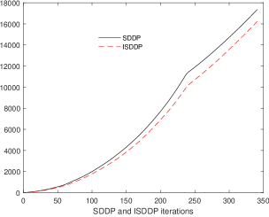
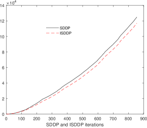
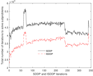
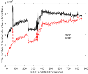
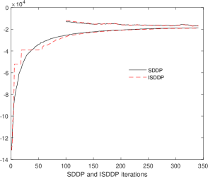
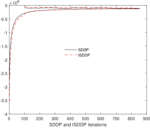
Figure 1: Top plots: cumulative CPU time (in seconds), middle plots: total number of iterations to solve subproblems, bottom plots: upper and lower bounds. Left plots: $M=100,$ $T=10$, $n=50$, right plots: $M=100,$ $T=30$, and $n=50$.

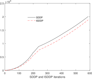
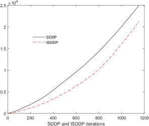
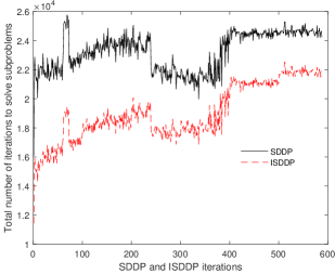
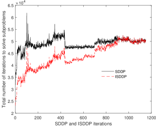
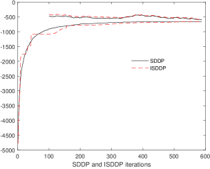
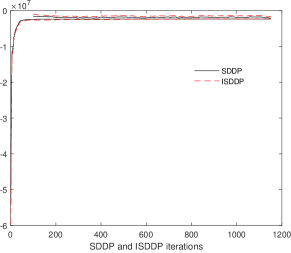
Figure 2: Top plots: cumulative CPU time (in seconds), middle plots: total number of iterations to solve subproblems, bottom plots: upper and lower bounds. Left plots: $M=50,$ $T=20$, $n=50$, right plots: $M=50,$ $T=40$, and $n=10$.

7 Conclusion

We have introduced the first inexact variant of SDDP to solve stochastic convex dynamic programming equations. We have shown that the method solves these equations for vanishing noises.

It would be interesting to consider the following extensions of this work:

• derive inexact cuts for problems with nondifferentiable cost and constraint functions;

• build cuts in the backward pass on the basis of approximate solutions which are not necessarily feasible;

• apply ISDDP to other real-life applications, testing several strategies for the sequence of error terms $(\delta_{t}^{k},\varepsilon_{t}^{k})$ or the maximal number of iterations for the LP solver used to solve the subproblems along the iterations of ISDDP.

Appendix

Proof of Theorem 4.3.

(i) We show (46) for $t=2,\ldots,T+1$, and all node $n$ of stage $t-1$ by backward induction on $t$. The relation holds for $t=T+1$. Now assume that it holds for $t+1$ for some $t\in\{2,\ldots,T\}$. Let us show that it holds for $t$. Take a node $n$ of stage $t-1$. Observe that the sequence $\mathcal{Q}_{t}(x_{n}^{k})-\mathcal{Q}_{t}^{k}(x_{n}^{k})$ is almost surely bounded and nonnegative. Therefore it has almost surely a nonnegative limit inferior and a finite limit superior. Let $\mathcal{S}_{n}=\{k:n_{t}^{k}=n\}$ be the iterations where the sampled scenario passes through node $n$. For $k\in\mathcal{S}_{n}$ we have $0\leq\mathcal{Q}_{t}(x_{n}^{k})-\mathcal{Q}_{t}^{k}(x_{n}^{k})$ and

(87) $$\begin{array}[]{l}\mathcal{Q}_{t}(x_{n}^{k})-\mathcal{Q}_{t}^{k}(x_{n}^{k})\leq\mathcal{Q}_{t}(x_{n}^{k})-\mathcal{C}_{t}^{k}(x_{n}^{k})\\ \leq\displaystyle{\bar{\varepsilon}}+\sum_{m\in C(n)}p_{m}\Big{[}\mathfrak{Q}_{t}(x_{n}^{k},\xi_{m})-{\underline{\mathfrak{Q}}}_{t}^{k}(x_{n}^{k},\xi_{m})\Big{]}\\ \leq\displaystyle{\bar{\varepsilon}}+\sum_{m\in C(n)}p_{m}\Big{[}\mathfrak{Q}_{t}(x_{n}^{k},\xi_{m})-{\underline{\mathfrak{Q}}}_{t}^{k-1}(x_{n}^{k},\xi_{m})\Big{]}\\ \leq\displaystyle{\bar{\varepsilon}}+\delta_{t}^{k}+\sum_{m\in C(n)}p_{m}\Big{[}\mathfrak{Q}_{t}(x_{n}^{k},\xi_{m})-\langle c_{m},x_{m}^{k}\rangle-\mathcal{Q}_{t+1}^{k-1}(x_{m}^{k})\Big{]}\\ \leq\displaystyle{\bar{\varepsilon}}+{\bar{\delta}}+\sum_{m\in C(n)}p_{m}\Big{[}\underbrace{\mathfrak{Q}_{t}(x_{n}^{k},\xi_{m})-\langle c_{m},x_{m}^{k}\rangle-\mathcal{Q}_{t+1}(x_{m}^{k})}_{\leq 0\mbox{ by definition of }\mathfrak{Q}_{t}\mbox{ and }x_{m}^{k}}+\mathcal{Q}_{t+1}(x_{m}^{k})-\mathcal{Q}_{t+1}^{k-1}(x_{m}^{k})\Big{]}\\ \leq\displaystyle{\bar{\varepsilon}}+{\bar{\delta}}+\sum_{m\in C(n)}p_{m}\Big{[}\mathcal{Q}_{t+1}(x_{m}^{k})-\mathcal{Q}_{t+1}^{k-1}(x_{m}^{k})\Big{]}.\end{array}$$

Using the induction hypothesis, we have for every $m\in C(n)$ that

$$\varlimsup_{k\rightarrow+\infty}\mathcal{Q}_{t+1}(x_{m}^{k})-\mathcal{Q}_{t+1}^{k}(x_{m}^{k})\leq({\bar{\delta}}+{\bar{\varepsilon}})(T-t).$$

In virtue of Lemma 4.1, this implies

(88) $$\varlimsup_{k\rightarrow+\infty}\mathcal{Q}_{t+1}(x_{m}^{k})-\mathcal{Q}_{t+1}^{k-1}(x_{m}^{k})\leq({\bar{\delta}}+{\bar{\varepsilon}})(T-t),$$

which, plugged into (87), gives

(89) $$\varlimsup_{k\rightarrow+\infty,k\in\mathcal{S}_{n}}\mathcal{Q}_{t}(x_{n}^{k})-\mathcal{Q}_{t}^{k}(x_{n}^{k})\leq({\bar{\delta}}+{\bar{\varepsilon}})(T-t+1).$$

Now let us show by contradiction that $\varlimsup_{k\rightarrow+\infty}\mathcal{Q}_{t}(x_{n}^{k})-\mathcal{Q}_{t}^{k}(x_{n}^{k})\leq({\bar{\delta}}+{\bar{\varepsilon}})(T-t+1)$. If this relation does not hold then there exists $\varepsilon_{0}>0$ such that there is an infinite set of iterations $k$ satisfying $\mathcal{Q}_{t}(x_{n}^{k})-\mathcal{Q}_{t}^{k}(x_{n}^{k})>({\bar{\delta}}+{\bar{\varepsilon}})(T-t+1)+\varepsilon_{0}$ and by monotonicity, there is also an infinite set of iterations $k$ in the set $K=\{k\geq 1:\mathcal{Q}_{t}(x_{n}^{k})-\mathcal{Q}_{t}^{k-1}(x_{n}^{k})>({\bar{\delta}}+{\bar{\varepsilon}})(T-t+1)+\varepsilon_{0}\}$. Let $k_{1}<k_{2}<...$ be these iterations: $K=\{k_{1},k_{2},\ldots,\}$. Let $y_{n}^{k}$ be the random variable which takes the value 1 if $k\in\mathcal{S}_{n}$ and $0$ otherwise. Due to Assumptions (A0)-(A2), random variables $y_{n}^{k_{1}},y_{n}^{k_{2}},\ldots,$ are i.i.d. and have the distribution of $y_{n}^{1}$. Therefore by the Strong Law of Large Numbers we get $\frac{1}{N}\displaystyle\sum_{j=1}^{N}y_{n}^{k_{j}}\xrightarrow{N\rightarrow+\infty}\mathbb{E}[y_{n}^{1}]>0\mbox{ a.s.}$ Now let $z_{1}<z_{2}<\ldots$ be the iterations in $\mathcal{S}_{n}$: $\mathcal{S}_{n}=\{z_{1},z_{2},\ldots\}$. Relation (89) can be written $\varlimsup_{k\rightarrow+\infty}\mathcal{Q}_{t}(x_{n}^{z_{k}})-\mathcal{Q}_{t}^{z_{k}}(x_{n}^{z_{k}})\leq({\bar{\delta}}+{\bar{\varepsilon}})(T-t+1),$ which, using Lemma 4.1, implies $\varlimsup_{k\rightarrow+\infty}\mathcal{Q}_{t}(x_{n}^{z_{k}})-\mathcal{Q}_{t}^{z_{k-1}}(x_{n}^{z_{k}})\leq({\bar{\delta}}+{\bar{\varepsilon}})(T-t+1).$ Using the fact that $z_{k}\geq z_{k-1}+1$, we deduce that $\varlimsup_{k\rightarrow+\infty,k\in\mathcal{S}_{n}}\mathcal{Q}_{t}(x_{n}^{k})-\mathcal{Q}_{t}^{k-1}(x_{n}^{k})=\varlimsup_{k\rightarrow+\infty}\mathcal{Q}_{t}(x_{n}^{z_{k}})-\mathcal{Q}_{t}^{z_{k}-1}(x_{n}^{z_{k}})\leq\varlimsup_{k\rightarrow+\infty}\mathcal{Q}_{t}(x_{n}^{z_{k}})-\mathcal{Q}_{t}^{z_{k-1}}(x_{n}^{z_{k}})\leq({\bar{\delta}}+{\bar{\varepsilon}})(T-t+1).$ Therefore, there can only be a finite number of iterations that are both in $K$ and in $\mathcal{S}_{n}$. This gives $\frac{1}{N}\displaystyle\sum_{j=1}^{N}y_{n}^{k_{j}}\xrightarrow{N\rightarrow+\infty}0\mbox{ a.s.}$ and we obtain the desired contradiction.

(ii) Using (87), we obtain for every $t=2,\ldots,T$, and every node $n$ of stage $t-1$, that

(90) $$0\leq\sum_{m\in C(n)}p_{m}\Big{[}c_{m}^{T}x_{m}^{k}+\mathcal{Q}_{t+1}(x_{m}^{k})\Big{]}-\mathcal{Q}_{t}(x_{n}^{k})\leq{\bar{\delta}}+{\bar{\varepsilon}}+\sum_{m\in C(n)}p_{m}\Big{[}\mathcal{Q}_{t+1}(x_{m}^{k})-\mathcal{Q}_{t+1}^{k-1}(x_{m}^{k})\Big{]}.$$

Therefore $\varliminf_{k\rightarrow+\infty}\sum_{m\in C(n)}p_{m}\Big{[}c_{m}^{T}x_{m}^{k}+\mathcal{Q}_{t+1}(x_{m}^{k})\Big{]}-\mathcal{Q}_{t}(x_{n}^{k})\geq 0$ and using (88) we get

$$\varlimsup_{k\rightarrow+\infty}\sum_{m\in C(n)}p_{m}\Big{[}c_{m}^{T}x_{m}^{k}+\mathcal{Q}_{t+1}(x_{m}^{k})\Big{]}-\mathcal{Q}_{t}(x_{n}^{k})\leq({\bar{\delta}}+{\bar{\varepsilon}})(T-t+1).$$

(iii) We have

(91) $$\begin{array}[]{lll}\mathcal{Q}_{1}(x_{0})\geq{\underline{\mathfrak{Q}}}_{1}^{k-1}(x_{0},\xi_{1})&\geq&c_{1}^{T}x_{1}^{k}+\mathcal{Q}_{2}^{k-1}(x_{1}^{k})-\delta_{1}^{k}\\ &\geq&-{\bar{\delta}}+\mathcal{Q}_{1}(x_{0})+\mathcal{Q}_{2}^{k-1}(x_{1}^{k})-\mathcal{Q}_{2}(x_{1}^{k}).\end{array}$$

Using (91) and (88) with $t=1$, we obtain (iii).

Additional parameters for ISDDP. For ISDDP, the maximal number of iterations allowed for Mosek LP solver to solve subproblems along the iterations of ISDDP is given in Table 2.

ISDDP iteration $[1,20]$ $[21,50]$ $[51,100]$ LP solver maximal number of iterations at $t$ $\left\lceil(0.4+0.6\frac{(t-2)}{T-2})I_{\max}\right\rceil$ $\left\lceil(0.45+0.55\frac{(t-2)}{T-2})I_{\max}\right\rceil$ $\left\lceil(0.5+0.5\frac{(t-2)}{T-2})I_{\max}\right\rceil$

ISDDP iteration $[101,200]$ $[201,300]$ $[301,400]$ LP solver maximal number of iterations at $t$ $\left\lceil(0.55+0.45\frac{(t-2)}{T-2})I_{\max}\right\rceil$ $\left\lceil(0.6+0.4\frac{(t-2)}{T-2})I_{\max}\right\rceil$ $\left\lceil(0.65+0.35\frac{(t-2)}{T-2})I_{\max}\right\rceil$

ISDDP iteration $[401,500]$ $[501,600]$ $[601,700]$ LP solver maximal number of iterations at $t$ $\left\lceil(0.7+0.3\frac{(t-2)}{T-2})I_{\max}\right\rceil$ $\left\lceil(0.75+0.25\frac{(t-2)}{T-2})I_{\max}\right\rceil$ $\left\lceil(0.8+0.2\frac{(t-2)}{T-2})I_{\max}\right\rceil$

ISDDP iteration $[701,800]$ $[801,900]$ $>900$ LP solver maximal number of iterations at $t$ $\left\lceil(0.85+0.15\frac{(t-2)}{T-2})I_{\max}\right\rceil$ $\left\lceil(0.9+0.1\frac{(t-2)}{T-2})I_{\max}\right\rceil$ $I_{\max}$

Table 2: Maximal number of iterations for Mosek LP solver for solving backward and forward passes subproblems as a function of stage $t\geq 2$, ISDDP iteration, and the number $I_{\max}$ of iterations used to solve subproblems with SDDP with high accuracy. In this table, $\left\lceil x\right\rceil$ is the smallest integer larger than or equal to $x$.

References

- [1] E. D. Andersen and K. Andersen, The MOSEK optimization toolbox for MATLAB manual. Version 7.0, 2013. https://www.mosek.com/.
- [2] J. Benders, Partitioning Procedures for Solving Mixed-Variables Programming Problems, Nmer. Math., 4 (1962), pp. 238–252.
- [3] J. Birge, Decomposition and partitioning methods for multistage stochastic linear programs, Oper. Res., 33 (1985), pp. 989–1007.
- [4] P. Girardeau, V. Leclere, and A. Philpott, On the convergence of decomposition methods for multistage stochastic convex programs, Mathematics of Operations Research, 40 (2015), pp. 130–145.
- [5] V. Guigues, Convergence analysis of sampling-based decomposition methods for risk-averse multistage stochastic convex programs, SIAM Journal on Optimization, 26 (2016), pp. 2468–2494.
- [6] V. Guigues, Dual dynamic programing with cut selection: Convergence proof and numerical experiments, European Journal of Operational Research, 258 (2017), pp. 47–57.
- [7] V. Guigues and M. Bandarra, Single cut and multicut sddp with cut selection for multistage stochastic linear programs: convergence proof and numerical experiments, Available at https://arxiv.org/abs/1902.06757, (2019).
- [8] V. Guigues and W. Römisch, Sampling-based decomposition methods for multistage stochastic programs based on extended polyhedral risk measures, SIAM J. Optim., 22 (2012), pp. 286–312.
- [9] V. Guigues and W. Römisch, SDDP for multistage stochastic linear programs based on spectral risk measures, Oper. Res. Lett., 40 (2012), pp. 313–318.
- [10] V. Guigues, W. Tekaya, and M. Lejeune, Regularized decomposition methods for deterministic and stochastic convex optimization and application to portfolio selection with direct transaction and market impact costs, Optimization OnLine, (2017).
- [11] V. Kozmik and D. Morton, Evaluating policies in risk-averse multi-stage stochastic programming, Mathematical Programming, 152 (2015), pp. 275–300.
- [12] D. McDaniel and M. Devine, A modified Benders’ Partitioning Algorithm for Mixed Integer Programming, Management Science, 24 (1977), pp. 312–319.
- [13] M. Pereira and L. Pinto, Multi-stage stochastic optimization applied to energy planning, Math. Program., 52 (1991), pp. 359–375.
- [14] A. Philpott and V. de Matos, Dynamic sampling algorithms for multi-stage stochastic programs with risk aversion, European Journal of Operational Research, 218 (2012), pp. 470–483.
- [15] A. B. Philpott and Z. Guan, On the convergence of stochastic dual dynamic programming and related methods, Oper. Res. Lett., 36 (2008), pp. 450–455.
- [16] A. Shapiro, Analysis of stochastic dual dynamic programming method, European Journal of Operational Research, 209 (2011), pp. 63–72.
- [17] A. Shapiro, W. Tekaya, J. da Costa, and M. Soares, Risk neutral and risk averse stochastic dual dynamic programming method, European Journal of Operational Research, 224 (2013), pp. 375–391.
- [18] G. Zakeri, A. Philpott, and D. Ryan, Inexact Cuts in Benders Decomposition, SIAM Journal on Optimization, 10 (2000), pp. 643–657.
- [19] J. Zou, S. Ahmed, and X. Sun, Stochastic dual dynamic integer programming, Optimization Online, (2017).