3D Surface Reconstruction by Pointillism

Abstract

The objective of this work is to infer the 3D shape of an object from a single image. We use sculptures as our training and test bed, as these have great variety in shape and appearance.

To achieve this we build on the success of multiple view geometry (MVG) which is able to accurately provide correspondences between images of 3D objects under varying viewpoint and illumination conditions, and make the following contributions: first, we introduce a new loss function that can harness image-to-image correspondences to provide a supervisory signal to train a deep network to infer a depth map. The network is trained end-to-end by differentiating through the camera. Second, we develop a processing pipeline to automatically generate a large scale multi-view set of correspondences for training the network. Finally, we demonstrate that we can indeed obtain a depth map of a novel object from a single image for a variety of sculptures with varying shape/texture, and that the network generalises at test time to new domains (e.g. synthetic images).

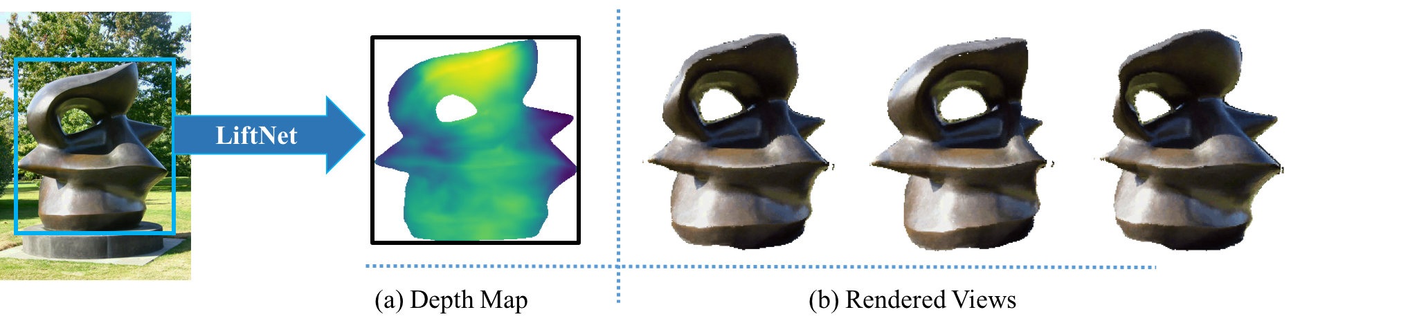
Figure 1: Given this image of the Spindle Piece by Henry Moore, LiftNet predicts the 3D shape of the sculpture via a depth map (a), where blue is further away and yellow nearer, and thereby enables new views to be rendered (b). LiftNet is trained self-supervised on real images using correspondences without any knowledge of depth or camera parameters.

1 Introduction

Humans are able to effortlessly perceive 3D shape of a previously unseen object from a single image – or at least we have the impression that we do this. For example for a piecewise smooth sculpture such as the one by Henry Moore in Fig. 1, we know where there are concavities, convexities and saddles, as well as where there are holes and sharp points. How this is achieved has long been studied in computer vision in terms of geometric cues from the silhouette [1], the texture [2, 3, 4], self-shadows, specularities [5], shading [6, 7], chiaroscuro [8], etc.

In this paper our objective is to be able to reconstruct such objects from a single image. Deep learning has significantly boosted progress in 3D reconstruction from single images, but so far methods have mostly depended on the availability of synthetic 3D training examples, or using a single class, or pre-processing the data using SfM and MVS to extract depth. In contrast, our self-supervised approach is to learn directly from real images, capitalizing on many years of research on MVG [9, 10, 11, 12] that is able to automatically determine matching views of a 3D object and generate point correspondences, without requiring any explicit 3D information as supervision.

The key idea is to use image-to-image point correspondences to provide a training loss on the depth map predicted by a CNN, called LiftNet. This is illustrated in figure 2. Suppose we are attempting to infer the depth of the object in a source view, and there are a number of image point correspondences available between the source view and a target view (where a correspondence is defined by the projection of a 3D surface point into the source and target views). A correspondence can be computed in two ways. First, it can be computed using matching methods from MVG (such as SIFT, and epipolar geometry). This method does not involve using the depth of the surface and we treat these correspondences as ground truth. Second, it can be computed by inferring the depth of the point in the source view and projecting the 3D point into the target view. If the CNN correctly predicts the depth of the points in the source view, then the projected points will coincide with the ground truth correspondences in the target view; however, if the the depth prediction is incorrect, then the distance between the projected and corresponding points – the re-projection error – defines a loss that can be used to train the network.

Of course, the correspondences between two views of a particular sculpture only provide constraints at those points on the surface – and correspondences will mainly be found at surface texture, surface discontinuities, and boundaries [13], i.e. not uniformly across the surface. However, for each sculpture there are multiple pairs of images; and each pair can ‘probe’ (and constrain) different points on the surface according to its correspondences. Finally, and most importantly, the network must learn to predict correspondences not just for a particular sculpture, but for all the sculptures (and all their view pairs) in the training set – and we have 170K training pairs and around 31M training correspondences. The only way it can solve this task is to infer 3D shape for each image.

To this end, we formulate a new deep learning framework for extracting 3D shape which is similar to the artistic pointillist style. Analogously to how pointillists build up colour variation in an image from dots of discrete colour, we use points in correspondence between images of an object in order to train a network over time to learn the 3D shape of the object.

Contributions. This work presents three contributions: first, to use corresponding points to formulate a differentiable loss on the object shape that can be used to train a network from scratch (Section 3). The formulation includes differentiating through the camera to train the network end-to-end.

The second contribution is a pipeline based on MVG for automatically extracting robust correspondences between multiple pairs of images of a sculpture (Section 4). We use these correspondences to train the network on real images, without ground truth 3D depth information. This is done entirely automatically and is the first system to our knowledge to learn to predict shape end-to-end for a set of objects by using correspondences and geometry in this manner.

The final contribution is our experimental results in Section 5, which demonstrate that the trained network can not only predict depth for the given domain but also generalises to synthetic data, allowing its generalisation capability to be evaluated quantitatively.

2 Related Work

Depth Prediction.

The ability to learn depth using a deep learning framework was introduced by [14], who use a dataset of ground truth depth and RGB image pairs to train a network to predict depth. This has been improved on with better architectures in [15, 16] and generalised to ordinal relationships in [17, 18].

A recent set of works have considered how to extract the 3D depth of a scene between pairs of images without knowing the camera motion or depth [19, 20, 21, 22]. This is done by predicting both depth and cameras in the network. This information is then used to transform one view and the photometric error between the generated image and the ground truth is used to train the network. These works require that the two images be very similar, such that the photometric error gives a robust and sensible loss. As a result, the images come from stereo datasets or consecutive video frames, such that the relative appearance change is small. On the other hand, our approach uses point correspondences directly, and consequently the images can vary dramatically in illumination, texture, size, position, etc. and our loss is robust to these changes.

3D Shape Prediction.

Going beyond depth prediction, which is view based, the entire 3D shape of the object can be reconstructed from multiple views by using strong supervision from the known 3D geometry to predict a voxel [23, 24] or point cloud [25, 26, 27] representation. Alternatively, the supervision can be from photo consistency or silhouette constraints [28, 29, 30, 31, 32]. However, these methods require knowledge of the camera parameters in order to enforce the geometric constraints.

These methods have been extended to deal with natural images in the work of [33, 34, 35], but [33] still requires a synthetic dataset on which to train their network which is then fine-tuned on real images. [34] uses structure from motion (SfM)/multi-view stereo (MVS) [9] from a video sequence as the ground truth 3D shape on which to train their network for reconstructing a finite set of classes; [35] extends this idea to unordered image collection of historic landmarks by using many images of the given landmark. In our case, we are not restricted to a finite set of classes, and do not require a video sequence or many images of the same scene in order to obtain a dense reconstruction, but instead train from the available correspondences directly, and these correspondences only need to exist over a handful of images. As a result, our approach can be used with far fewer samples of each landmark or sculpture.

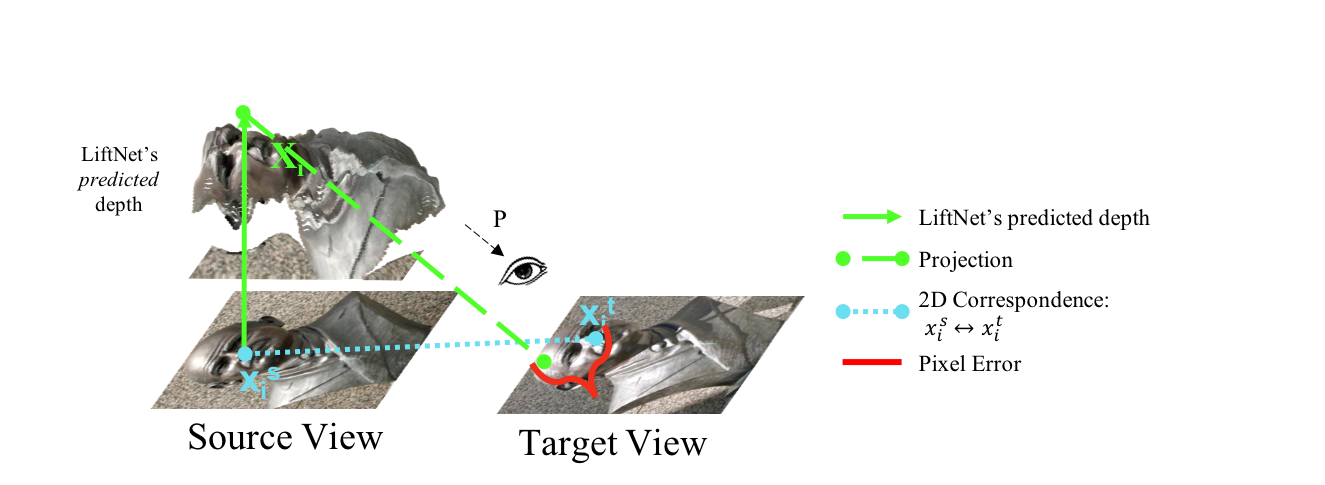
Figure 2: An illustration of the training loss: $\mathcal{L}_{\text{corr}}$. Given ${{\mathchoice{\mbox{\boldmath$\displaystyle\bf x$}}{\mbox{\boldmath$\textstyle\bf x$}}{\mbox{\boldmath$\scriptstyle\bf x$}}{\mbox{\boldmath$\scriptscriptstyle\bf x$}}_{i}^{s}}}\leftrightarrow{\mathchoice{\mbox{\boldmath$\displaystyle\bf x$}}{\mbox{\boldmath$\textstyle\bf x$}}{\mbox{\boldmath$\scriptstyle\bf x$}}{\mbox{\boldmath$\scriptscriptstyle\bf x$}}_{i}^{t}}$ and the best camera $\textstyle\tt P$, we minimise the error between $\textstyle\tt P$${\mathchoice{\mbox{\boldmath$\displaystyle\bf X$}}{\mbox{\boldmath$\textstyle\bf X$}}{\mbox{\boldmath$\scriptstyle\bf X$}}{\mbox{\boldmath$\scriptscriptstyle\bf X$}}_{i}}$ and ${\mathchoice{\mbox{\boldmath$\displaystyle\bf x$}}{\mbox{\boldmath$\textstyle\bf x$}}{\mbox{\boldmath$\scriptstyle\bf x$}}{\mbox{\boldmath$\scriptscriptstyle\bf x$}}_{i}^{t}}$. The depth $d_{i}$ value of ${\mathchoice{\mbox{\boldmath$\displaystyle\bf X$}}{\mbox{\boldmath$\textstyle\bf X$}}{\mbox{\boldmath$\scriptstyle\bf X$}}{\mbox{\boldmath$\scriptscriptstyle\bf X$}}_{i}}$ is LiftNet’s predicted depth for the source view at ${{\mathchoice{\mbox{\boldmath$\displaystyle\bf x$}}{\mbox{\boldmath$\textstyle\bf x$}}{\mbox{\boldmath$\scriptstyle\bf x$}}{\mbox{\boldmath$\scriptscriptstyle\bf x$}}_{i}^{s}}}$. If $d_{i}$ were correctly predicted by LiftNet there would be no error as ${\mathchoice{\mbox{\boldmath$\displaystyle\bf X$}}{\mbox{\boldmath$\textstyle\bf X$}}{\mbox{\boldmath$\scriptstyle\bf X$}}{\mbox{\boldmath$\scriptscriptstyle\bf X$}}_{i}}$ would project to ${\mathchoice{\mbox{\boldmath$\displaystyle\bf x$}}{\mbox{\boldmath$\textstyle\bf x$}}{\mbox{\boldmath$\scriptstyle\bf x$}}{\mbox{\boldmath$\scriptscriptstyle\bf x$}}_{i}^{t}}$; the image distance between the projected point and ${\mathchoice{\mbox{\boldmath$\displaystyle\bf x$}}{\mbox{\boldmath$\textstyle\bf x$}}{\mbox{\boldmath$\scriptstyle\bf x$}}{\mbox{\boldmath$\scriptscriptstyle\bf x$}}_{i}^{t}}$ provides the training loss. As the network’s prediction improves, the distance reduces to zero.

3 Approach

The goal is to recover 3D structure from a single image by predicting a depth map, but without requiring ground truth 3D information in training. In this section we first define the loss functions used to train the network. Then the LiftNet architecture is described in Section 3.3. In the following we assume that correspondences between images are available (as described in Section 4).

As introduced in Section 1, the depth predicted by the LiftNet CNN in the source view is supervised by using point correspondences as follows: (i) let the set of correspondences be denoted as ${{\mathchoice{\mbox{\boldmath$\displaystyle\bf x$}}{\mbox{\boldmath$\textstyle\bf x$}}{\mbox{\boldmath$\scriptstyle\bf x$}}{\mbox{\boldmath$\scriptscriptstyle\bf x$}}_{i}^{s}}}\leftrightarrow{\mathchoice{\mbox{\boldmath$\displaystyle\bf x$}}{\mbox{\boldmath$\textstyle\bf x$}}{\mbox{\boldmath$\scriptstyle\bf x$}}{\mbox{\boldmath$\scriptscriptstyle\bf x$}}_{i}^{t}}$, where ${{\mathchoice{\mbox{\boldmath$\displaystyle\bf x$}}{\mbox{\boldmath$\textstyle\bf x$}}{\mbox{\boldmath$\scriptstyle\bf x$}}{\mbox{\boldmath$\scriptscriptstyle\bf x$}}_{i}^{s}}}$ are the points in the source view, and ${\mathchoice{\mbox{\boldmath$\displaystyle\bf x$}}{\mbox{\boldmath$\textstyle\bf x$}}{\mbox{\boldmath$\scriptstyle\bf x$}}{\mbox{\boldmath$\scriptscriptstyle\bf x$}}_{i}^{t}}$ the points in the target view. (ii) Then in the source view we can determine the 3D points ${\mathchoice{\mbox{\boldmath$\displaystyle\bf X$}}{\mbox{\boldmath$\textstyle\bf X$}}{\mbox{\boldmath$\scriptstyle\bf X$}}{\mbox{\boldmath$\scriptscriptstyle\bf X$}}_{i}}$ that project to ${{\mathchoice{\mbox{\boldmath$\displaystyle\bf x$}}{\mbox{\boldmath$\textstyle\bf x$}}{\mbox{\boldmath$\scriptstyle\bf x$}}{\mbox{\boldmath$\scriptscriptstyle\bf x$}}_{i}^{s}}}$ (since the network gives the depth of each point). (iii) Since we know the correspondence between ${\mathchoice{\mbox{\boldmath$\displaystyle\bf X$}}{\mbox{\boldmath$\textstyle\bf X$}}{\mbox{\boldmath$\scriptstyle\bf X$}}{\mbox{\boldmath$\scriptscriptstyle\bf X$}}_{i}}$ and ${\mathchoice{\mbox{\boldmath$\displaystyle\bf x$}}{\mbox{\boldmath$\textstyle\bf x$}}{\mbox{\boldmath$\scriptstyle\bf x$}}{\mbox{\boldmath$\scriptscriptstyle\bf x$}}_{i}^{t}}$ we can compute the best camera that projects the 3D points ${\mathchoice{\mbox{\boldmath$\displaystyle\bf X$}}{\mbox{\boldmath$\textstyle\bf X$}}{\mbox{\boldmath$\scriptstyle\bf X$}}{\mbox{\boldmath$\scriptscriptstyle\bf X$}}_{i}}$ into the target view. (iv) If the 3D shape has been predicted perfectly, then the 3D points ${\mathchoice{\mbox{\boldmath$\displaystyle\bf X$}}{\mbox{\boldmath$\textstyle\bf X$}}{\mbox{\boldmath$\scriptstyle\bf X$}}{\mbox{\boldmath$\scriptscriptstyle\bf X$}}_{i}}$ will project perfectly onto ${\mathchoice{\mbox{\boldmath$\displaystyle\bf x$}}{\mbox{\boldmath$\textstyle\bf x$}}{\mbox{\boldmath$\scriptstyle\bf x$}}{\mbox{\boldmath$\scriptscriptstyle\bf x$}}_{i}^{t}}$. If they do not, then this reprojection error provides a loss that can be minimized to train the network. The resulting loss is defined as:

$$\mathcal{L}_{\text{corr}}=\frac{1}{N}\sum_{i=1}^{N}d_{R}(\mathchoice{\mbox{\boldmath$\displaystyle\tt P$}}{\mbox{\boldmath$\textstyle\tt P$}}{\mbox{\boldmath$\scriptstyle\tt P$}}{\mbox{\boldmath$\scriptscriptstyle\tt P$}}\mathchoice{\mbox{\boldmath$\displaystyle\bf X$}}{\mbox{\boldmath$\textstyle\bf X$}}{\mbox{\boldmath$\scriptstyle\bf X$}}{\mbox{\boldmath$\scriptscriptstyle\bf X$}}_{i},\mathchoice{\mbox{\boldmath$\displaystyle\bf x$}}{\mbox{\boldmath$\textstyle\bf x$}}{\mbox{\boldmath$\scriptstyle\bf x$}}{\mbox{\boldmath$\scriptscriptstyle\bf x$}}_{i}^{t});$$ (1)

where $d_{R}(.,.)$ denotes the Euclidean ($L_{2}$) pixel distance between vectors subject to a robustness function $R$.

This loss is a useful constraint, as it enforces important properties of the object, such as concavities and convexities. Moreover, this can be done for any pair of images for which correspondences can be obtained. There is no requirement that the images be photometrically consistent – e.g. lighting, texture, position etc. can vary dramatically between views.

Finally, a robustness term $R$ is added (Section 3.2), as the 2D correspondences may be noisy (as explained in Section 4).

3.1 Point Correspondence Loss $\mathcal{L}_{\text{corr}}$

We minimise the projection error between ${\mathchoice{\mbox{\boldmath$\displaystyle\bf X$}}{\mbox{\boldmath$\textstyle\bf X$}}{\mbox{\boldmath$\scriptstyle\bf X$}}{\mbox{\boldmath$\scriptscriptstyle\bf X$}}_{i}}$ and ${\mathchoice{\mbox{\boldmath$\displaystyle\bf x$}}{\mbox{\boldmath$\textstyle\bf x$}}{\mbox{\boldmath$\scriptstyle\bf x$}}{\mbox{\boldmath$\scriptscriptstyle\bf x$}}_{i}^{t}}$ using the best camera $\textstyle\tt P$: $\frac{1}{N}\sum_{i=1}^{N}d_{R}(\mathchoice{\mbox{\boldmath$\displaystyle\tt P$}}{\mbox{\boldmath$\textstyle\tt P$}}{\mbox{\boldmath$\scriptstyle\tt P$}}{\mbox{\boldmath$\scriptscriptstyle\tt P$}}\mathchoice{\mbox{\boldmath$\displaystyle\bf X$}}{\mbox{\boldmath$\textstyle\bf X$}}{\mbox{\boldmath$\scriptstyle\bf X$}}{\mbox{\boldmath$\scriptscriptstyle\bf X$}}_{i},\mathchoice{\mbox{\boldmath$\displaystyle\bf x$}}{\mbox{\boldmath$\textstyle\bf x$}}{\mbox{\boldmath$\scriptstyle\bf x$}}{\mbox{\boldmath$\scriptscriptstyle\bf x$}}_{i}^{t})$. The steps are as follows:

A. Choose the camera.

This work assumes an affine camera and an orthogonal coordinate system in the source view, which is why ${\mathchoice{\mbox{\boldmath$\displaystyle\bf X$}}{\mbox{\boldmath$\textstyle\bf X$}}{\mbox{\boldmath$\scriptstyle\bf X$}}{\mbox{\boldmath$\scriptscriptstyle\bf X$}}_{i}}=[x_{i}^{s},y_{i}^{s},d_{i},1]^{T}$ projects to ${{\mathchoice{\mbox{\boldmath$\displaystyle\bf x$}}{\mbox{\boldmath$\textstyle\bf x$}}{\mbox{\boldmath$\scriptstyle\bf x$}}{\mbox{\boldmath$\scriptscriptstyle\bf x$}}_{i}^{s}}}=(x_{i}^{s},y_{i}^{s})$ in the source view. As has been noted previously [9, 36, 37], the affine case is a very stable and useful approximation to perspective projection. The reader is referred to the supplementary material for a detailed review of this camera model. However, we note that the ideas presented here (e.g. the method of differentiating the camera) generalise in a straight forward manner to the perspective case.

B. Determine the camera.

We first determine the camera matrix $\textstyle\tt P$ by solving the system of equations ${\mathchoice{\mbox{\boldmath$\displaystyle\bf x$}}{\mbox{\boldmath$\textstyle\bf x$}}{\mbox{\boldmath$\scriptstyle\bf x$}}{\mbox{\boldmath$\scriptscriptstyle\bf x$}}_{i}^{t}}$ $=\mathchoice{\mbox{\boldmath$\displaystyle\tt P$}}{\mbox{\boldmath$\textstyle\tt P$}}{\mbox{\boldmath$\scriptstyle\tt P$}}{\mbox{\boldmath$\scriptscriptstyle\tt P$}}$ ${\mathchoice{\mbox{\boldmath$\displaystyle\bf X$}}{\mbox{\boldmath$\textstyle\bf X$}}{\mbox{\boldmath$\scriptstyle\bf X$}}{\mbox{\boldmath$\scriptscriptstyle\bf X$}}_{i}}$ for $\textstyle\tt P$. We know which values ${\mathchoice{\mbox{\boldmath$\displaystyle\bf X$}}{\mbox{\boldmath$\textstyle\bf X$}}{\mbox{\boldmath$\scriptstyle\bf X$}}{\mbox{\boldmath$\scriptscriptstyle\bf X$}}_{i}}$ and ${\mathchoice{\mbox{\boldmath$\displaystyle\bf x$}}{\mbox{\boldmath$\textstyle\bf x$}}{\mbox{\boldmath$\scriptstyle\bf x$}}{\mbox{\boldmath$\scriptscriptstyle\bf x$}}_{i}^{t}}$ should correspond because LiftNet’s prediction is simply a depth map, so ${{\mathchoice{\mbox{\boldmath$\displaystyle\bf x$}}{\mbox{\boldmath$\textstyle\bf x$}}{\mbox{\boldmath$\scriptstyle\bf x$}}{\mbox{\boldmath$\scriptscriptstyle\bf x$}}_{i}^{s}}}=(x_{i}^{s},y_{i}^{s})$ in pixels maps to ${\mathchoice{\mbox{\boldmath$\displaystyle\bf X$}}{\mbox{\boldmath$\textstyle\bf X$}}{\mbox{\boldmath$\scriptstyle\bf X$}}{\mbox{\boldmath$\scriptscriptstyle\bf X$}}_{i}}=[x_{i}^{s},y_{i}^{s},d_{i},1]^{T}$ ($d_{i}$ is the depth prediction at that point) and we know, via the correspondences, that ${{\mathchoice{\mbox{\boldmath$\displaystyle\bf x$}}{\mbox{\boldmath$\textstyle\bf x$}}{\mbox{\boldmath$\scriptstyle\bf x$}}{\mbox{\boldmath$\scriptscriptstyle\bf x$}}_{i}^{s}}}\leftrightarrow{\mathchoice{\mbox{\boldmath$\displaystyle\bf x$}}{\mbox{\boldmath$\textstyle\bf x$}}{\mbox{\boldmath$\scriptstyle\bf x$}}{\mbox{\boldmath$\scriptscriptstyle\bf x$}}_{i}^{t}}$, so ${\mathchoice{\mbox{\boldmath$\displaystyle\bf X$}}{\mbox{\boldmath$\textstyle\bf X$}}{\mbox{\boldmath$\scriptstyle\bf X$}}{\mbox{\boldmath$\scriptscriptstyle\bf X$}}_{i}}$ maps to ${\mathchoice{\mbox{\boldmath$\displaystyle\bf x$}}{\mbox{\boldmath$\textstyle\bf x$}}{\mbox{\boldmath$\scriptstyle\bf x$}}{\mbox{\boldmath$\scriptscriptstyle\bf x$}}_{i}^{t}}$. This gives the following system of equations:

$$\begin{bmatrix}x_{1}^{t}&\dots&x_{N}^{t}\\ y_{1}^{t}&\dots&y_{N}^{t}\\ \end{bmatrix}=\mathchoice{\mbox{\boldmath$\displaystyle\tt P$}}{\mbox{\boldmath$\textstyle\tt P$}}{\mbox{\boldmath$\scriptstyle\tt P$}}{\mbox{\boldmath$\scriptscriptstyle\tt P$}}\begin{bmatrix}x_{1}^{s}&\dots&x_{N}^{s}\\ y_{1}^{s}&\dots&y_{N}^{s}\\ d_{1}&\dots&d_{N}\\ 1&\dots&1\\ \end{bmatrix}.$$ (2)

However, directly solving the system of equations would be problematic due to the effect of outliers, (e.g. noise in the data). A standard approach to deal with noise is to make use of RANSAC [38]. This method solves a system of equations by finding a solution that satisfies the most constraints. The satisfied constraints are called inliers, the others outliers. In our case, we want to find $\textstyle\tt P$ such that the maximum number of pairs ${\mathchoice{\mbox{\boldmath$\displaystyle\bf X$}}{\mbox{\boldmath$\textstyle\bf X$}}{\mbox{\boldmath$\scriptstyle\bf X$}}{\mbox{\boldmath$\scriptscriptstyle\bf X$}}_{i}}$ and ${\mathchoice{\mbox{\boldmath$\displaystyle\bf x$}}{\mbox{\boldmath$\textstyle\bf x$}}{\mbox{\boldmath$\scriptstyle\bf x$}}{\mbox{\boldmath$\scriptscriptstyle\bf x$}}_{i}^{t}}$ satisfy the condition $|{\mathchoice{\mbox{\boldmath$\displaystyle\bf x$}}{\mbox{\boldmath$\textstyle\bf x$}}{\mbox{\boldmath$\scriptstyle\bf x$}}{\mbox{\boldmath$\scriptscriptstyle\bf x$}}_{i}^{t}}-\mathchoice{\mbox{\boldmath$\displaystyle\tt P$}}{\mbox{\boldmath$\textstyle\tt P$}}{\mbox{\boldmath$\scriptstyle\tt P$}}{\mbox{\boldmath$\scriptscriptstyle\tt P$}}{\mathchoice{\mbox{\boldmath$\displaystyle\bf X$}}{\mbox{\boldmath$\textstyle\bf X$}}{\mbox{\boldmath$\scriptstyle\bf X$}}{\mbox{\boldmath$\scriptscriptstyle\bf X$}}_{i}}|_{2}<T$ for some threshold $T$. Given the set of inliers $\mathchoice{\mbox{\boldmath$\displaystyle\bf X$}}{\mbox{\boldmath$\textstyle\bf X$}}{\mbox{\boldmath$\scriptstyle\bf X$}}{\mbox{\boldmath$\scriptscriptstyle\bf X$}}_{i_{\text{inliers}}},\mathchoice{\mbox{\boldmath$\displaystyle\bf x$}}{\mbox{\boldmath$\textstyle\bf x$}}{\mbox{\boldmath$\scriptstyle\bf x$}}{\mbox{\boldmath$\scriptscriptstyle\bf x$}}_{i_{\text{inliers}}}^{t}$, a new system of linear equations is constructed: $\mathchoice{\mbox{\boldmath$\displaystyle\bf x$}}{\mbox{\boldmath$\textstyle\bf x$}}{\mbox{\boldmath$\scriptstyle\bf x$}}{\mbox{\boldmath$\scriptscriptstyle\bf x$}}_{i_{\text{inliers}}}^{t}=\mathchoice{\mbox{\boldmath$\displaystyle\tt P$}}{\mbox{\boldmath$\textstyle\tt P$}}{\mbox{\boldmath$\scriptstyle\tt P$}}{\mbox{\boldmath$\scriptscriptstyle\tt P$}}\mathchoice{\mbox{\boldmath$\displaystyle\bf X$}}{\mbox{\boldmath$\textstyle\bf X$}}{\mbox{\boldmath$\scriptstyle\bf X$}}{\mbox{\boldmath$\scriptscriptstyle\bf X$}}_{i_{\text{inliers}}}$.

C. Compute the loss.

Given $\textstyle\tt P$, all points $\mathchoice{\mbox{\boldmath$\displaystyle\bf X$}}{\mbox{\boldmath$\textstyle\bf X$}}{\mbox{\boldmath$\scriptstyle\bf X$}}{\mbox{\boldmath$\scriptscriptstyle\bf X$}}_{i}$ are projected into the target view and the error between their projection and known location ${\mathchoice{\mbox{\boldmath$\displaystyle\bf x$}}{\mbox{\boldmath$\textstyle\bf x$}}{\mbox{\boldmath$\scriptstyle\bf x$}}{\mbox{\boldmath$\scriptscriptstyle\bf x$}}_{i}^{t}}$ is computed. The loss is then as given in (1).

D. Differentiate through the camera.

In order to train the network end to end, it is necessary to compute the derivative $\frac{\partial\mathchoice{\mbox{\boldmath$\displaystyle\tt P$}}{\mbox{\boldmath$\textstyle\tt P$}}{\mbox{\boldmath$\scriptstyle\tt P$}}{\mbox{\boldmath$\scriptscriptstyle\tt P$}}}{\partial d_{i}}$. To do this, we re-write the system of equations such that $\textstyle\tt P$ is explicitly a function of $x_{i_{\text{inliers}}}^{t}$/$\mathchoice{\mbox{\boldmath$\displaystyle\bf X$}}{\mbox{\boldmath$\textstyle\bf X$}}{\mbox{\boldmath$\scriptstyle\bf X$}}{\mbox{\boldmath$\scriptscriptstyle\bf X$}}_{i_{\text{inliers}}}$ such that computing the derivative is straightforward. For ease of notation, the matrix of inliers $\mathchoice{\mbox{\boldmath$\displaystyle\bf X$}}{\mbox{\boldmath$\textstyle\bf X$}}{\mbox{\boldmath$\scriptstyle\bf X$}}{\mbox{\boldmath$\scriptscriptstyle\bf X$}}_{i_{\text{inliers}}}$ is referred to as $\textstyle\tt X$ and of inliers $\mathchoice{\mbox{\boldmath$\displaystyle\tt x$}}{\mbox{\boldmath$\textstyle\tt x$}}{\mbox{\boldmath$\scriptstyle\tt x$}}{\mbox{\boldmath$\scriptscriptstyle\tt x$}}_{i_{\text{inliers}}}$ as $\textstyle\tt x$ from now on. The pseudo-inverse $\mathchoice{\mbox{\boldmath$\displaystyle\tt X$}}{\mbox{\boldmath$\textstyle\tt X$}}{\mbox{\boldmath$\scriptstyle\tt X$}}{\mbox{\boldmath$\scriptscriptstyle\tt X$}}^{+}$ is computed using the singular value decomposition (SVD) [39]. (If the SVD of a matrix $\textstyle\tt A$ is $\mathchoice{\mbox{\boldmath$\displaystyle\tt A$}}{\mbox{\boldmath$\textstyle\tt A$}}{\mbox{\boldmath$\scriptstyle\tt A$}}{\mbox{\boldmath$\scriptscriptstyle\tt A$}}=\mathchoice{\mbox{\boldmath$\displaystyle\tt U$}}{\mbox{\boldmath$\textstyle\tt U$}}{\mbox{\boldmath$\scriptstyle\tt U$}}{\mbox{\boldmath$\scriptscriptstyle\tt U$}}\mathchoice{\mbox{\boldmath$\displaystyle\tt\Sigma$}}{\mbox{\boldmath$\textstyle\tt\Sigma$}}{\mbox{\boldmath$\scriptstyle\tt\Sigma$}}{\mbox{\boldmath$\scriptscriptstyle\tt\Sigma$}}\mathchoice{\mbox{\boldmath$\displaystyle\tt V$}}{\mbox{\boldmath$\textstyle\tt V$}}{\mbox{\boldmath$\scriptstyle\tt V$}}{\mbox{\boldmath$\scriptscriptstyle\tt V$}}^{T}$ then its pseudo inverse can be written as $\mathchoice{\mbox{\boldmath$\displaystyle\tt A$}}{\mbox{\boldmath$\textstyle\tt A$}}{\mbox{\boldmath$\scriptstyle\tt A$}}{\mbox{\boldmath$\scriptscriptstyle\tt A$}}^{+}=\mathchoice{\mbox{\boldmath$\displaystyle\tt V$}}{\mbox{\boldmath$\textstyle\tt V$}}{\mbox{\boldmath$\scriptstyle\tt V$}}{\mbox{\boldmath$\scriptscriptstyle\tt V$}}\mathchoice{\mbox{\boldmath$\displaystyle\tt\Sigma$}}{\mbox{\boldmath$\textstyle\tt\Sigma$}}{\mbox{\boldmath$\scriptstyle\tt\Sigma$}}{\mbox{\boldmath$\scriptscriptstyle\tt\Sigma$}}^{+}\mathchoice{\mbox{\boldmath$\displaystyle\tt U$}}{\mbox{\boldmath$\textstyle\tt U$}}{\mbox{\boldmath$\scriptstyle\tt U$}}{\mbox{\boldmath$\scriptscriptstyle\tt U$}}^{T}$.) Then the system of equations can be re-written as:

$$\tt x =\mathchoice{\mbox{\boldmath$\displaystyle\tt P$}}{\mbox{\boldmath$\textstyle\tt P$}}{\mbox{\boldmath$\scriptstyle\tt P$}}{\mbox{\boldmath$\scriptscriptstyle\tt P$}}\mathchoice{\mbox{\boldmath$\displaystyle\tt X$}}{\mbox{\boldmath$\textstyle\tt X$}}{\mbox{\boldmath$\scriptstyle\tt X$}}{\mbox{\boldmath$\scriptscriptstyle\tt X$}}$$ (3)

$$\mathchoice{\mbox{\boldmath$\displaystyle\tt x$}}{\mbox{\boldmath$\textstyle\tt x$}}{\mbox{\boldmath$\scriptstyle\tt x$}}{\mbox{\boldmath$\scriptscriptstyle\tt x$}}^{T} =\mathchoice{\mbox{\boldmath$\displaystyle\tt X$}}{\mbox{\boldmath$\textstyle\tt X$}}{\mbox{\boldmath$\scriptstyle\tt X$}}{\mbox{\boldmath$\scriptscriptstyle\tt X$}}^{T}\mathchoice{\mbox{\boldmath$\displaystyle\tt P$}}{\mbox{\boldmath$\textstyle\tt P$}}{\mbox{\boldmath$\scriptstyle\tt P$}}{\mbox{\boldmath$\scriptscriptstyle\tt P$}}^{T}$$ (4)

$$(\mathchoice{\mbox{\boldmath$\displaystyle\tt X$}}{\mbox{\boldmath$\textstyle\tt X$}}{\mbox{\boldmath$\scriptstyle\tt X$}}{\mbox{\boldmath$\scriptscriptstyle\tt X$}}^{T})^{+}\mathchoice{\mbox{\boldmath$\displaystyle\tt x$}}{\mbox{\boldmath$\textstyle\tt x$}}{\mbox{\boldmath$\scriptstyle\tt x$}}{\mbox{\boldmath$\scriptscriptstyle\tt x$}}^{T} \approx(\mathchoice{\mbox{\boldmath$\displaystyle\tt X$}}{\mbox{\boldmath$\textstyle\tt X$}}{\mbox{\boldmath$\scriptstyle\tt X$}}{\mbox{\boldmath$\scriptscriptstyle\tt X$}}^{T})^{+}\mathchoice{\mbox{\boldmath$\displaystyle\tt X$}}{\mbox{\boldmath$\textstyle\tt X$}}{\mbox{\boldmath$\scriptstyle\tt X$}}{\mbox{\boldmath$\scriptscriptstyle\tt X$}}^{T}\mathchoice{\mbox{\boldmath$\displaystyle\tt P$}}{\mbox{\boldmath$\textstyle\tt P$}}{\mbox{\boldmath$\scriptstyle\tt P$}}{\mbox{\boldmath$\scriptscriptstyle\tt P$}}^{T}\approx\mathchoice{\mbox{\boldmath$\displaystyle\tt P$}}{\mbox{\boldmath$\textstyle\tt P$}}{\mbox{\boldmath$\scriptstyle\tt P$}}{\mbox{\boldmath$\scriptscriptstyle\tt P$}}^{T}$$ (5)

$$(\mathchoice{\mbox{\boldmath$\displaystyle\tt V$}}{\mbox{\boldmath$\textstyle\tt V$}}{\mbox{\boldmath$\scriptstyle\tt V$}}{\mbox{\boldmath$\scriptscriptstyle\tt V$}}\mathchoice{\mbox{\boldmath$\displaystyle\tt\Sigma$}}{\mbox{\boldmath$\textstyle\tt\Sigma$}}{\mbox{\boldmath$\scriptstyle\tt\Sigma$}}{\mbox{\boldmath$\scriptscriptstyle\tt\Sigma$}}^{+}\mathchoice{\mbox{\boldmath$\displaystyle\tt U$}}{\mbox{\boldmath$\textstyle\tt U$}}{\mbox{\boldmath$\scriptstyle\tt U$}}{\mbox{\boldmath$\scriptscriptstyle\tt U$}}^{T})\mathchoice{\mbox{\boldmath$\displaystyle\tt x$}}{\mbox{\boldmath$\textstyle\tt x$}}{\mbox{\boldmath$\scriptstyle\tt x$}}{\mbox{\boldmath$\scriptscriptstyle\tt x$}}^{T} =\mathchoice{\mbox{\boldmath$\displaystyle\tt P$}}{\mbox{\boldmath$\textstyle\tt P$}}{\mbox{\boldmath$\scriptstyle\tt P$}}{\mbox{\boldmath$\scriptscriptstyle\tt P$}}^{T}$$ (6)

Note that because the system of equations in (2) is over-constrained then of course this is not an exact solution, but the pseudo-inverse solves the system of equations in the least-squares sense [39] which is what we require. Also, note that because the outliers are ignored when computing $\textstyle\tt P$ due to RANSAC, we can ignore them in this computation and only consider the inliers. This gives the forward pass.

To perform the backward pass, it is necessary to compute the derivative $\frac{\partial\mathchoice{\mbox{\boldmath$\displaystyle\tt P$}}{\mbox{\boldmath$\textstyle\tt P$}}{\mbox{\boldmath$\scriptstyle\tt P$}}{\mbox{\boldmath$\scriptscriptstyle\tt P$}}}{\partial d_{i}}$. This is a straight-forward application of the product and chain rule, except for the computation of the SVD. However, previous work (e.g. [40]) has demonstrated how to compute these derivatives. As a result we can back-propagate through the computation of $\textstyle\tt P$ to the estimation of the height values $d_{i}$. This is achieved in practice using standard layers in a neural network library (e.g. PyTorch [41]). Note that computing the gradients for $\textstyle\tt U$, $\textstyle\tt V$ could lead to potential instability if $\mathchoice{\mbox{\boldmath$\displaystyle\tt X$}}{\mbox{\boldmath$\textstyle\tt X$}}{\mbox{\boldmath$\scriptstyle\tt X$}}{\mbox{\boldmath$\scriptscriptstyle\tt X$}}^{T}$ is not full rank or has repeated singular values; however, this was not a problem in practice.

Discussion.

We note that our method computes $\textstyle\bf d$ up to an overall affine ambiguity. This amounts to a scaling and shearing in the depth prediction. This ambiguity is seen in human vision, as humans have been shown to reconstruct objects (such as vases) up to an affine transformation in depth [42, 43]. It is hypothesised that this difficulty arises from the fact that, assuming Lambertian reflectance and given a single image, the surface of an object can only be recovered up to a generalized bas-relief ambiguity [44].

3.2 Robustness

As the correspondences and segmentations will be noisy, it is necessary that the loss function is robust to these errors. To do this we use a smooth function to weight the errors [45] so that errors above a threshold $\tau$ are given a constant cost: $\mathcal{R}(x)=\begin{cases}\frac{1}{2}x^{2}(1-\frac{x^{2}}{2\tau^{2}}),&\text{if }x^{2}\leq\tau^{2}\\ \tau^{2}/4,&\text{otherwise}\par\end{cases}$.

3.3 Architecture

The architecture used is based on the U-Net [46] variant of pix2pix [47]. This architecture includes skip connections in order to maintain high level detail. However, we incorporate two modifications. First the last activation is replaced by a tanh layer to enforce that the output lies between $[-1,1]$. We impose this range so that the predicted depth does not grow too large, making training unstable. As LiftNet learns depth up to a scaling factor in depth, this in no way constrains the types of surfaces that LiftNet can describe. Second, the nearest neighbour upsampler is replaced by a bilinear upsampler. This mitigates against pixelated effects [48, 49]. Please refer to the supp. material for full details.

4 The Sculpture Dataset

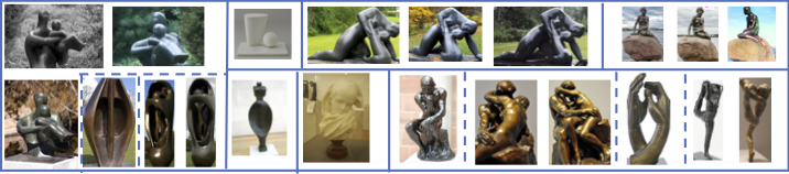
(a) The images are organised by artist (solid lines) into clusters (dashed lines). Note the variety and complexity of the sculptures: in shape, materials, lighting, and viewpoint.

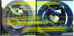
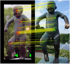
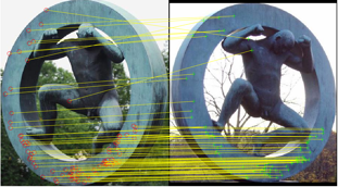
(b) Sample correspondences for pairs of images. The images may be taken at different times of year, in different contexts/illumination conditions and the material itself may change over time due to weather.

Figure 3: The Sculpture dataset. Note that this is only a tiny subset of the clusters and a fraction of the number of images within a cluster. Please refer to the supp. material for more examples.

We assemble a large scale dataset of images of sculptures for training and testing by combining multiple public datasets [50, 13, 51, 52] and downloading additional images from the web. The dataset incorporates a wide variety of artists, styles and materials. It is divided at the artist level to prevent any information bleeding between the sets. Table 1 gives the number of artists and works used as well as the train/val/test splits.

The dataset includes multiple works (sculptures) by different artists (sculptors) organised into a set of clusters. Within a cluster, the images are of the same sculpture (shape), but there may be multiple instances of the sculpture, some made of different material. The utility of the dataset is that within a cluster there are many point correspondences between image pairs that can be used for training the network. Fig. 3 shows a sample of sculptures, correspondences and an example cluster.

Table 1: Dataset statistics for the Sculpture dataset. Note the large number of artists and works. This results in a large variety of styles and shapes that LiftNet must contend with. A total of 31M point correspondences ($\approx 181$ correspondences $\times$ $169K$ pairs) are automatically generated and used to train LiftNet.

	Train	Val	Test	All
#Artists	138	7	1	143
#Works	1031	27	129	1187
#Matching Pairs	168726	552	13166	182K
Avg # Correspondences per Pair	181	223	174	181

The remainder of this section describes the steps used to download, prepare, and obtain the image pair correspondences of the dataset. Additional details are given in the supplementary material.

Image extraction. We combine multiple sculpture datasets: [50, 13, 51, 52] and download additional images from the web.

Obtaining segmentations. To segment the images, RefineNET [53] is trained on 2000 hand-labelled sculptures by artists Rodin and Henry Moore. It achieves a $0.94$ IoU score and $0.97$ accuracy on the validation dataset. This is used for a wide variety of images and it generalises well to new sculptures.

Obtaining correspondences. The final step is to determine a valid set of correspondences. The OpenMVG pipeline [54] is used to extract an initial dense list of correspondences between pairs of images. The segmentation from RefineNET above is then used to mask out correspondences from the irrelevant background parts of the image. Additionally those correspondences that do not satisfy the affine fundamental matrix, which is computed using RANSAC, are removed. Finally, those image pairs that can be mapped by an affine homography (i.e. a 2D transformation between images) are thrown out, as they will not provide a constraint on 3D structure.

Despite these post-processing steps, there will still be noise in the correspondences, motivating the use of a robust cost in our losses explained in Section 3.

5 Experiments

A challenge of our framework is to determine its prediction quality, as there is no ground truth depth information for the automatically collected Sculpture dataset. To this end, LiftNet is evaluated in multiple environments and scenarios. First, we use a realistic synthetic dataset of sculptures SketchFab [55] and ShapeNet [56] for which we can determine ground truth information and thereby correspondences between views; these are introduced below. LiftNet is then trained using these generated correspondences and compared to a baseline trained to explicitly regress depth on Section 5.3 and Section 5.4. Second, we train LiftNet on real data: the Sculpture dataset. This network is then compared to a number of self-supervised and supervised methods in Section 5.5. This evaluation is performed on two datasets: first it is performed on Scanned, a dataset of scanned objects. Second, the evaluation is performed on SketchFab (despite the domain gap between real and synthetic images the network generalises to this new domain). Finally, it is evaluated qualitatively on the Sculpture dataset  in Section 5.6.

5.1 Datasets, evaluation metrics, and baselines

The SketchFab and ShapeNet datasets.

SketchFab is a large dataset of synthetic 3D models of sculptures generated using photogrammetry. There are 425 sculptures divided into 372/20/33 train/val/test sculptures. ShapeNet consists of multiple semantic classes, each of which is divided into train/val/test using the given splits. For evaluation, five views of each SketchFab object and $10$ views of each ShapeNet object are rendered in Blender [57] using orthographic projection and the ground truth depth extracted. The SketchFab objects are viewed with azimuth $\in[0^{\circ},120^{\circ}]$, elevation $0^{\circ}$ whereas ShapeNet objects are viewed with azimuth $\in[0^{\circ},360^{\circ}]$ and elevation $\in[-45^{\circ},45^{\circ}]$. As the depth and cameras of the renders are known, the ground truth correspondences between images can be determined by projecting the depth in the source view into the target view.

Scanned.

Additional data is collected from the $80$ sculpture videos of [58]. These are taken ‘in-the-wild’ with a hand-held camera. Of these videos, 11 objects are chosen and the sculpture region segmented. This gives 208 images for testing.

Evaluation metrics.

The results are reported using multiple metrics: the $L_{1}$ error, root mean squared error, relative $L_{1}$ error, and squared rel. difference [14]. To evaluate the depth prediction, it is necessary to take into account the ambiguity in the $z$ axis (the depth prediction). This is done by allowing for a scaling/translation in depth. Thus for all models (including those trained on ground truth depth), when reporting results, the depth prediction $d_{\text{pred}}$ for an image is first normalised by $d^{*}_{\text{pred}}=\alpha(d_{\text{pred}}-\beta_{1})+\beta_{2}$ where $\beta_{1}$ is the median of $d_{\text{pred}}$, $\beta_{2}$ is the median of $d_{\text{gt}}$ and $\alpha$ allows for a scaling in depth: $\alpha=\sum_{xy}(d_{\text{pred}}*d_{\text{gt}})/\sum_{xy}(d_{\text{pred}}^{2})$. ($d_{gt}$ denotes ground truth and $\sum_{xy}$ denotes summation over pixel locations.)

Baselines.

In the evaluation on synthetic data, we compare against a supervised baseline, explicitly trained to regress depth. We use the same network (e.g. pix2pix) as LiftNet. The MSELoss is used but after first accounting for a scaling and translation in depth as follows. If the depth predicted is $d_{\text{pred}}$ then the normalised depth is $d^{*}_{\text{pred}}=\alpha(d_{\text{pred}}-\beta_{1})+\beta_{2}$, which is computed as described above for the evaluation metrics. The loss is then $|d^{*}_{\text{pred}}-d_{gt}|_{2}$.

5.2 Training

The network is trained as follows. Two images with correspondences are sampled from the dataset; one is designated source, the other target. The source view is then input to LiftNet, which predicts the depth at all pixels. The predicted depth of the foreground pixels $d_{i}$, concatenated with the $x_{i}$,$y_{i}$ position of the pixel in the image give the 3D points in the source view $\mathchoice{\mbox{\boldmath$\displaystyle\bf X$}}{\mbox{\boldmath$\textstyle\bf X$}}{\mbox{\boldmath$\scriptstyle\bf X$}}{\mbox{\boldmath$\scriptscriptstyle\bf X$}}_{i}=[x_{i},y_{i},d_{i},1]^{T}$. The correspondence loss – $\mathcal{L}_{\text{corr}}$ – is then imposed on these 3D points.

At test time (visualised in Fig. 4), an image is simply input to the network. This gives the depth prediction for all pixels. For visualisation purposes, the sculpture (the foreground pixels) are segmented from the background and only the depth values at these foreground pixels is shown.

The models are trained on a single Titan GPU in PyTorch [59]. They take about half a day to train.

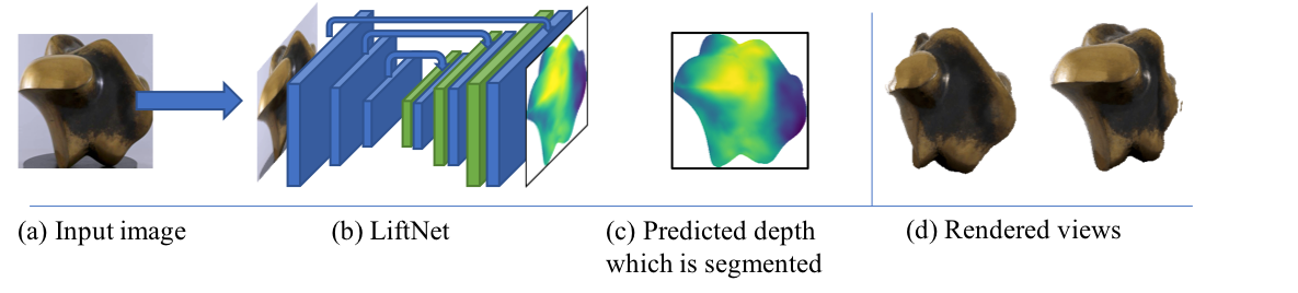
Figure 4: The test time pipeline for LiftNet. (a) An image is selected from the test dataset and input to LiftNet (Section 3.3). (b) LiftNet gives a depth map prediction at all points. (c-d) The rendered depth is then segmented and visualised at new views. (This is a sample result on the test set.)

All models trained on the Sculpture dataset are trained as follows. The models are trained with SGD, a learning rate of $1e^{-5}$, and momentum of $0.9$. The gradients are clamped to $\pm 5$. These models are trained until the correspondence error on the Sculpture dataset’s validation set stops decreasing. When trained on SketchFab or ShapeNet, models are trained with SGD a learning rate of $1e^{-3}$, and momentum of $0.9$. The gradients are clamped to $\pm 5$. They are trained until the correspondence error on the validation set stops decreasing or a maximum of $200$ epochs.

5.3 Quantitative results on ShapeNet

In this section, we evaluate LiftNet on ShapeNet. In order to test the correspondence loss, $50$ correspondences per pair of images of an object are randomly chosen and fixed using the known depth and camera transformation. This gives the training set.

The results are reported in Table 2 and LiftNet is compared to training the same network architecture (i.e. pix2pix) but directly regressing the ground truth depth up to a scaling and translation in depth as described above.

Table 2: Comparison of ‘LiftNet trained on ShapeNet correspondences’ to ‘pix2pix trained using a MSE loss on ShapeNet’. The error measure is RMSE (x100).

	rif.	boo.	bus	bed	spe.	cab.	lam.	cha.	tra.	pla.	tab.	dis.	mot.	car	wat.	pho.	sofa
pix2pix	1.71	2.14	1.89	2.16	1.66	1.76	1.44	1.87	1.71	0.90	2.52	2.28	1.71	1.33	1.36	1.56	2.19
LiftNet	2.03	1.94	2.11	1.21	1.29	1.21	1.38	0.94	2.06	1.05	1.51	1.66	1.92	1.12	1.51	1.52	1.34

These results are perhaps surprising, as LiftNet does better on multiple classes and comparably on most. Thus, training with a limited number of correspondences can yield comparable results to training with dense depth.

5.4 Quantitative results on SketchFab

In this section, LiftNet is evaluated on a synthetic dataset of sculptures, SketchFab, which has more varied shapes than ShapeNet. LiftNet is trained using ground truth correspondences for SketchFab for every pixel (i.e. dense points). LiftNet’s performance is then compared with the baseline methods trained with depth. As demonstrated in Table 4, our method performs similarly to the supervised method trained explicitly to regress depth. Qualitative results are given in the supplementary material.

While here we have used all points, for ShapeNet only $50$ correspondences was sufficient. Consequently, we additionally investigate in Table 3 the performance as a function of the number of training correspondences used per image and demonstrate that using a fraction of the available number of correspondences gives comparable results to using all. For example, using $100$ correspondences gives similar results – $0.175/0.254$ L1/RMSE error versus $0.175/0.255$; we can use $1.1\%$ of the correspondences and achieve comparable results to using all.

Table 3: Evaluation of LiftNet’s robustness to the number of training correspondences. Lower is better. These results demonstrate that using only 50 correspondences per training pair gives similar results to using all. Thus, sparse correspondences are sufficient for training LiftNet.

# Correspondences per Image	$L_{1}$	RMSE	$\frac{d^{*}-d_{gt}}{d_{gt}}$	$\frac{(d^{*}-d_{gt})^{2}}{d_{gt}}$
10	0.183	0.263	0.0673	0.0253
50	0.178	0.261	0.0650	0.0242
100	0.175	0.254	0.0640	0.0233
$\approx$9000	0.175	0.255	0.0641	0.0233

5.5 Quantitative results using real world data

Given the initial experiments on ShapeNet and SketchFab, which demonstrate that our loss is sufficient to learn about 3D and that using sparse correspondences is powerful, we turn our attention to using real-world, noisy data. The model is trained on the real-world images from the Sculpture dataset. However, as there is no large dataset of ground truth 3D sculptures, we evaluate on two datasets. First, we evaluate on real images using the Scanned dataset. Second we evaluate the model’s generalisation capabilities by evaluating on SketchFab. To perform well, the model must generalise to a new, synthetic domain which may require a challenging domain shift. However, in practice, the model seems robust enough to generalise to this domain.

Training. When training, the loss on the validation set decreases from $\approx 4.0$ to $\approx 3.4$, converging in $40K$ iterations.

Table 4: The performance of LiftNet evaluated on the SketchFab dataset. Across all metrics, lower is better.

Method	Trained with	Training Dataset	$L_{1}$	RMSE	$\frac{d^{*}-d_{gt}}{d_{gt}}$	$\frac{(d^{*}-d_{gt})^{2}}{d_{gt}}$
COLMAP [60]	Depth from SfM	Sculptures	0.195	0.284	0.0760	0.0291
LiftNet: $\mathcal{L}_{\text{Corr}}$ (no $R$)	Correspondences	Sculptures	0.190	0.277	0.0690	0.0269
LiftNet: $\mathcal{L}_{\text{Corr}}$	Correspondences	Sculptures	0.186	0.270	0.0677	0.0256
Zhou et. al. [21]	Photometric Error	Sculptures	0.202	0.291	0.0732	0.0297
Chen et al. [17]	Ground Truth Ordinal Depth	Depth-in-the-Wild	0.186	0.269	0.0680	0.0258
LiftNet: $\mathcal{L}_{\text{Corr}}$	Correspondences	SketchFab	0.175	0.254	0.0641	0.0233
pix2pix	Depth	SketchFab	0.173	0.254	0.0628	0.0226

Ablation Studies. The first step is to ensure that our loss does indeed enforce that LiftNet learns about depth. To perform this check, we evaluate LiftNet on the test set of SketchFab and evaluate the effect of adding each component: the correspondence loss $\mathcal{L}_{\text{corr}}$ and the robustness term $R$.

The results are reported in Table 4. From these results, it is clear that the correspondence loss provides a strong constraint on the predicted depth, which is improved by the robustness term.

Comparison to SfM. The benefit of our approach is that we do not require videos of the same object but instead can use unordered image collections and a small number of images per object. To demonstrate this, we compare to COLMAP [60]. COLMAP is run on the clusters and the recovered 3D used to train a model to explicitly regress depth. COLMAP failed for 77% of the clusters, as there are not sufficient images/correspondences for it to converge to a global solution. Table 4 and 5 compares the performance of the two methods. The proposed pipeline and LiftNet training are superior, due to (we assume): (1) more data for training, as no correspondences are thrown out; and (2) that the depth from COLMAP may be incorrect due to the small number of images per cluster, which may lead to an incorrect solution.

This experiment suggests that our method is additionally useful when fine-tuning a pre-trained model (e.g. with ground truth depth) on a new domain with only a few images per instance (e.g. lesser known landmarks, sculptures, etc.) as a SfM approach would fail given the sparse amount of information.

Table 5: The performance of LiftNet evaluated on the Scanned dataset. Across all metrics, lower is better.

Method	Trained with	Training Dataset	$L_{1}(cm)$	RMSE (cm)	$\frac{d^{*}-d_{gt}}{d_{gt}}$	$\frac{(d^{*}-d_{gt})^{2}}{d_{gt}}$
COLMAP [60]	Depth from SfM	Sculptures	9.5	11.8	0.0741	18.1
LiftNet: $\mathcal{L}_{\text{Corr}}$	Correspondences	Sculptures	9.4	11.6	0.0741	16.6
Zhou et. al. [21]	Photometric Error	Sculptures	9.8	12.1	0.0761	18.7
Chen et al. [17]	Ground Truth Ordinal Depth	Depth-in-the-Wild	9.3	11.7	0.0722	17.1

Comparison to other self-supervised approaches. The second hypothesis to test is whether our method is more robust than other self-supervised methods which rely on photometric consistency. We compare to the work of [21] by running their model on our dataset. However, we note that their method requires knowledge of the intrinsic camera parameters which we do not have. As a result, we assume the intrinsic camera parameters have focal length 0.7*W, and the principal point is (0.5W, 0.5H) (W/H are the width/height of the image). The results are reported in Table 4. As can be seen their model does poorly: this is presumably due to a number of challenging characteristics of the Sculpture dataset. First, as mentioned above the intrinsic camera parameters are not known and may change from image to image. Second, there are large changes in illumination, changes in context, changes in weather, etc. All of these characteristics make using a photometric loss not robust and lead to worse results.

Comparison to supervised approaches. Despite LiftNet doing better than comparable self-supervised approaches, as reported above, the next question is how does LiftNet compare to a method [17] trained with depth supervision. [17] is pre-trained on the NYU depth dataset [61] which contains 795 densely annotated images and fine-tuned on the depth-in-the-wild [17] which contains 5M images with ordinal relationships. As demonstrated in Table 4 and 5, LiftNet does comparably or better than this supervised baseline.

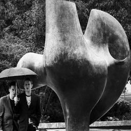
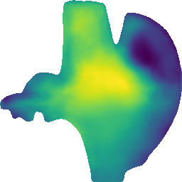
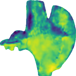
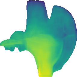
(a)

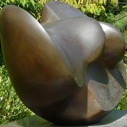
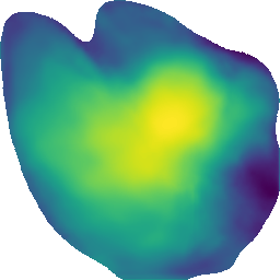
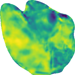
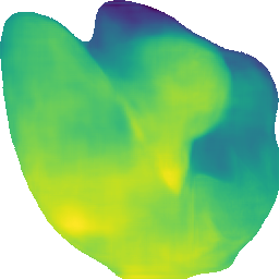
(b)

Figure 5: Reconstruction results for LiftNet (top), COLMAP (middle) and Chen et al. [17] (bottom), visualised using Open3D [62]. The input image is shown at the top, then the predicted depth (blue is further away, yellow nearer), and rendered 3D at multiple viewpoints. Zoom in for details. From these images, the following are demonstrated. First, Chen et al. learns a prior over the image that the bottom of the image is nearer and the top further away. This is demonstrated in (a) and further examples in the supp. material. Second, COLMAP’s depth predictions are noisy. Finally, LiftNet produces convincing depth maps which can be rendered at new views.

5.6 Qualitative Results on the Sculpture dataset

We demonstrate in Fig. 5 the predictions of LiftNet on the testing portion of the Sculpture dataset and compare them visually to two other methods: COLMAP and the supervised method [17]. We note that COLMAP performs poorly, presumably as there are very few training points. [17] produces reasonable results, as it is trained on a large dataset of outdoors images with supervision on relative depth in addition to NYU, but it has certain priors over the image (e.g. that points in the bottom of the image are always nearer than those in the top – as for most images the foreground is at the bottom of the image and sky at the top). Please see the supplementary material for more results.

6 Discussion

In this paper, we have introduced a framework for learning 3D shape using easily attainable sparse correspondences without depth supervision. Our insight is that we can make use of sparse correspondences, which can be obtained in much less constrained environments than approaches requiring photometric consistency. Given enough sparse correspondences across many instances, the network learns a dense depth prediction. The approach has been demonstrated on a challenging sculpture dataset of real images and a synthetic sculpture dataset with known ground truth information.

It is interesting to consider why this training scenario based on real images, and sculptures in particular, produces a network that performs well on real images and also generalizes to synthetic image. It is probably in part because the training data has natural augmentation – instances of a sculpture with the same shape may be made from different materials (bronze, marble) or have different texturing and appearance due to different weathering or illumination conditions. The network must learn to produce the same shape, irrespective of these multifarious conditions. This is a challenging learning problem but, if successful, then the network has correctly learnt to disentangle the material/appearance from the shape, and to pick out cues to shape from appearance. Thus it can generalize to objects with different materials, e.g. synthetic ones.

Acknowledgements.

The authors would like to thank Fatma Guney for helpful feedback and suggestions. This work was funded by an EPSRC studentship and EPSRC Programme Grant Seebibyte EP/M013774/1.

References

- [1] Koenderink, J.J.: What does the occluding contour tell us about solid shape? Perception 13 (1984) 321–330
- [2] Witkin, A.P.: Recovering surface shape and orientation from texture. Artificial intelligence 17(1-3) (1981) 17–45
- [3] Malik, J., Rosenholtz, R.: Computing local surface orientation and shape from texture for curved surfaces. IJCV 23(2) (1997) 149–168
- [4] Blake, A., Marinos, C.: Shape from texture: estimation, isotropy and moments. Artificial Intelligence 45(3) (1990) 323–380
- [5] Fleming, R.W., Torralba, A., Adelson, E.H.: Specular reflections and the perception of shape. Journal of Vision 4(9) (2004) 798–820
- [6] Zhang, R., Tsai, P.S., Cryer, J.E., Shah, M.: Shape-from-shading: a survey. IEEE PAMI 21(8) (1999) 690–706
- [7] Barron, J.T., Malik, J.: Shape, illumination, and reflectance from shading. IEEE PAMI (2015)
- [8] Koenderink, J.J., van Doorn, A.J.: Photometric invariants related to solid shape. Optica Acta 27(7) (1980) 981–996
- [9] Hartley, R.I., Zisserman, A.: Multiple View Geometry in Computer Vision. Second edn. Cambridge University Press, ISBN: 0521540518 (2004)
- [10] Lowe, D.: Distinctive image features from scale-invariant keypoints. IJCV 60(2) (2004) 91–110
- [11] Snavely, N., Seitz, S., Szeliski, R.: Photo tourism: exploring photo collections in 3D. Proc. ACM SIGGRAPH (3) (2006) 835–846
- [12] Schaffalitzky, F., Zisserman, A.: Multi-view matching for unordered image sets, or “how do i organize my holiday snaps?”. In: Proc. ECCV. Volume 1., Springer-Verlag (2002) 414–431
- [13] Arandjelović, R., Zisserman, A.: Name that sculpture. In: ACM International Conference on Multimedia Retrieval. (2012)
- [14] Eigen, D., Puhrsch, C., Fergus, R.: Depth map prediction from a single image using a multi-scale deep network. In: NIPS. (2014)
- [15] Laina, I., Rupprecht, C., Belagiannis, V., Tombari, F., Navab, N.: Deeper depth prediction with fully convolutional residual networks. In: 3D Vision (3DV), 2016 Fourth International Conference on. (2016)
- [16] Eigen, D., Fergus, R.: Predicting depth, surface normals and semantic labels with a common multi-scale convolutional architecture. In: Proc. CVPR. (2015)
- [17] Chen, W., Fu, Z., Yang, D., Deng, J.: Single-image depth perception in the wild. In: NIPS. (2016)
- [18] Zoran, D., Isola, P., Krishnan, D., Freeman, W.T.: Learning ordinal relationships for mid-level vision. In: Proc. ICCV. (2015)
- [19] Vijayanarasimhan, S., Ricco, S., Schmid, C., Sukthankar, R., Fragkiadaki, K.: Sfm-net: Learning of structure and motion from video. arXiv preprint arXiv:1704.07804 (2017)
- [20] Godard, C., Aodha, O.M., Brostow, G.J.: Unsupervised monocular depth estimation with left-right consistency. In: Proc. CVPR. (2017)
- [21] Zhou, T., Brown, M., Snavely, N., Lowe, D.G.: Unsupervised learning of depth and ego-motion from video. In: Proc. CVPR. (2017)
- [22] Ummenhofer, B., Zhou, H., Uhrig, J., Mayer, N., Ilg, E., Dosovitskiy, A., Brox, T.: Demon: Depth and motion network for learning monocular stereo. Proc. CVPR (2017)
- [23] Choy, C., Xu, D., Gwak, J., Chen, K., Savarese, S.: 3D-R2N2: A unified approach for single and multi-view 3D object reconstruction. In: Proc. ECCV. (Jul 2016)
- [24] Girdhar, R., Fouhey, D.F., Rodriguez, M., Gupta, A.: Learning a predictable and generative vector representation for objects. In: Proc. ECCV. (2016)
- [25] Fan, H., Su, H., Guibas, L.: A point set generation network for 3D object reconstruction from a single image. Proc. CVPR (2017)
- [26] Sinha, A., Unmesh, A., Huang, Q., Ramani, K.: Surfnet: Generating 3D shape surfaces using deep residual networks. In: Proc. CVPR. (2017)
- [27] Wu, J., Zhang, C., Xue, T., Freeman, B., Tenenbaum, J.: Learning a probabilistic latent space of object shapes via 3D generative-adversarial modeling. In: NIPS. (2016) 82–90
- [28] Soltani, A.A., Huang, H., Wu, J., Kulkarni, T.D., Tenenbaum, J.B.: Synthesizing 3D shapes via modeling multi-view depth maps and silhouettes with deep generative networks. In: Proc. CVPR. (2017)
- [29] Tulsiani, S., Zhou, T., Efros, A., Malik, J.: Multi-view supervision for single-view reconstruction via differentiable ray consistency. In: Proc. CVPR. (2017)
- [30] Rezende, D., Eslami, S.M.A., Mohamed, S., Battaglia, P., Jaderberg, M., Heess, N.: Unsupervised learning of 3D structure from images. In: NIPS. (2016) 4997–5005
- [31] Yan, X., Yang, J., Yumer, E., Guo, Y., Lee, H.: Perspective transformer nets: Learning single-view 3D object reconstruction without 3D supervision. In: NIPS. (2016)
- [32] Gadelha, M., Maji, S., Wang, R.: 3D shape induction from 2D views of multiple objects. arXiv preprint arXiv:1612.05872 (2016)
- [33] Zhu, R., Kiani, H., Wang, C., Lucey, S.: Rethinking reprojection: Closing the loop for pose-aware shape reconstruction from a single image. Proc. ICCV (2017)
- [34] Novotny, D., Larlus, D., Vedaldi, A.: Learning 3D object categories by looking around them. Proc. ICCV (2017)
- [35] Li, Z., Snavely, N.: MegaDepth: Learning single-view depth prediction from internet photos. In: Proc. CVPR. (2018)
- [36] Hong, J.H., Zach, C., Fitzgibbon, A., Cipolla, R.: Projective bundle adjustment from arbitrary initialization using the variable projection method. In: Proc. ECCV. (2016)
- [37] Hong, J.H., Zach, C., Fitzgibbon, A.: Revisiting the variable projection method for separable nonlinear least squares problems. In: Proc. CVPR. (2017)
- [38] Fischler, M.A., Bolles, R.C.: Random sample consensus: A paradigm for model fitting with applications to image analysis and automated cartography. Comm. ACM 24(6) (1981) 381–395
- [39] Strang, G.: Linear algebra and its applications. 2 edn. Academic Press, Inc. (1980)
- [40] Papadopoulo, T., Lourakis, M.I.: Estimating the jacobian of the singular value decomposition: Theory and applications. In: Proc. ECCV. (2000)
- [41] Paszke, A., Gross, S., Chintala, S., Chanan, G., Yang, E., DeVito, Z., Lin, Z., Desmaison, A., Antiga, L., Lerer, A.: Automatic differentiation in PyTorch. (2017)
- [42] Todd, J.T.: The visual perception of 3D shape. Trends in cognitive sciences 8(3) (2004) 115–121
- [43] Koenderink, J.J., Van Doorn, A.J., Kappers, A.M.: Surface perception in pictures. Perception & Psychophysics 52(5) (1992) 487–496
- [44] Belhumeur, P.N., Kriegman, D.J., Yuille, A.L.: The bas-relief ambiguity. IJCV 35(1) (1999) 33–44
- [45] Liwicki, S., Zach, C., Miksik, O., Torr, P.H.: Coarse-to-fine planar regularization for dense monocular depth estimation. In: Proc. ECCV. (2016)
- [46] Ronneberger, O., Fischer, P., Brox, T.: U-net: Convolutional networks for biomedical image segmentation. In: Proc. MICCAI. (2015)
- [47] Isola, P., Zhu, J.Y., Zhou, T., Efros, A.A.: Image-to-image translation with conditional adversarial networks. Proc. CVPR (2017)
- [48] Odena, A., Dumoulin, V., Olah, C.: Deconvolution and checkerboard artifacts. Distill (2016)
- [49] Chen, Q., Koltun, V.: Photographic image synthesis with cascaded refinement networks. In: Proc. ICCV. (2017)
- [50] Arandjelović, R., Zisserman, A.: Smooth object retrieval using a bag of boundaries. In: Proc. ICCV. (2011)
- [51] Fouhey, D.F., Gupta, A., Zisserman, A.: 3D shape attributes. In: Proc. CVPR. (2016)
- [52] Knapitsch, A., Park, J., Zhou, Q.Y., Koltun, V.: Tanks and temples: Benchmarking large-scale scene reconstruction. ACM Transactions on Graphics 36(4) (2017)
- [53] Lin, G., Milan, A., Shen, C., Reid, I.: Refinenet: Multi-path refinement networks with identity mappings for high-resolution semantic segmentation. Proc. CVPR (2017)
- [54] Moulon, P., Monasse, P., Marlet, R., Others: Openmvg. an open multiple view geometry library. https://github.com/openMVG/openMVG
- [55] Wiles, O., Zisserman, A.: Silnet : Single- and multi-view reconstruction by learning from silhouettes. In: Proc. BMVC. (2017)
- [56] Chang, A.X., Funkhouser, T., Guibas, L., Hanrahan, P., Huang, Q., Li, Z., Savarese, S., Savva, M., Song, S., Su, H., Xiao, J., Yi, L., Yu, F.: ShapeNet: An information-rich 3D model repository. Technical Report arXiv:1512.03012 [cs.GR] (2015)
- [57] Blender Online Community: Blender - a 3D modelling and rendering package. (2017)
- [58] Choi, S., Zhou, Q.Y., Miller, S., Koltun, V.: A large dataset of object scans. arXiv:1602.02481 (2016)
- [59] : Pytorch
- [60] Schönberger, J.L., Frahm, J.M.: Structure-from-motion revisited. In: Proc. CVPR. (2016)
- [61] Silberman, N., Hoiem, D., Kohli, P., Fergus, R.: Indoor segmentation and support inference from RGB-D images. In: Proc. ECCV. (2012)
- [62] Zhou, Q.Y., Park, J., Koltun, V.: Open3D: A modern library for 3D data processing. arXiv:1801.09847 (2018)