Evaluation Measures for Quantification: An Axiomatic Approach

Abstract

Quantification is the task of estimating, given a set $\sigma$ of unlabelled items and a set of classes $\mathcal{C}=\{c_{1},\ldots,c_{|\mathcal{C}|}\}$, the prevalence (or “relative frequency”) in $\sigma$ of each class $c_{i}\in\mathcal{C}$. While quantification may in principle be solved by classifying each item in $\sigma$ and counting how many such items have been labelled with $c_{i}$, it has long been shown that this “classify and count” (CC) method yields suboptimal quantification accuracy. As a result, quantification is no longer considered a mere byproduct of classification, and has evolved as a task of its own. While the scientific community has devoted a lot of attention to devising more accurate quantification methods, it has not devoted much to discussing what properties an evaluation measure for quantification (EMQ) should enjoy, and which EMQs should be adopted as a result. This paper lies down a number of interesting properties that an EMQ may or may not enjoy, discusses if (and when) each of these properties is desirable, surveys the EMQs that have been used so far, and discusses whether they enjoy or not the above properties. As a result of this investigation, some of the EMQs that have been used in the literature turn out to be severely unfit, while others emerge as closer to what the quantification community actually needs. However, a significant result is that no existing EMQ satisfies all the properties identified as desirable, thus indicating that more research is needed in order to identify (or synthesize) a truly adequate EMQ.

1 Introduction

Quantification (also known as “supervised prevalence estimation” (Barranquero et al., 2013), or “class prior estimation” (du Plessis et al., 2017)) is the task of estimating, given a set $\sigma$ of unlabelled items and a set of classes $\mathcal{C}=\{c_{1},\ldots,c_{|\mathcal{C}|}\}$, the relative frequency (or “prevalence”) $p(c_{i})$ of each class $c_{i}\in\mathcal{C}$, i.e., the fraction of items in $\sigma$ that belong to $c_{i}$. When each item belongs to exactly one class, since $0\leq p(c_{i})\leq 1$ and $\sum_{c_{i}\in\mathcal{C}}p(c_{i})=1$, $p$ is a distribution of the items in $\sigma$ across the classes in $\mathcal{C}$ (the true distribution), and quantification thus amounts to estimating $p$ (i.e., to computing a predicted distribution $\hat{p}$).

Quantification is important in many disciplines (such as e.g., market research, political science, the social sciences, and epidemiology) which usually deal with aggregate (as opposed to individual) data. In these contexts, classifying individual unlabelled instances is usually not a primary goal, while estimating the prevalence of the classes of interest in the data is. For instance, when classifying the tweets about a certain entity (e.g., a political candidate) as displaying either a Positive or a Negative stance towards the entity, we are usually not much interested in the class of a specific tweet: instead, we usually want to know the fraction of these tweets that belong to the class (Gao and Sebastiani, 2016).

Quantification may in principle be solved via classification, i.e., by classifying each item in $\sigma$ and counting, for all $c_{i}\in\mathcal{C}$, how many such items have been labelled with $c_{i}$. However, it has been shown in a multitude of works (see e.g., (Barranquero et al., 2015; Bella et al., 2010; Esuli and Sebastiani, 2015; Forman, 2008; Gao and Sebastiani, 2016; Hopkins and King, 2010)) that this “classify and count” (CC) method yields suboptimal quantification accuracy. Simply put, the reason of this suboptimality is that most classifiers are optimized for classification accuracy, and not for quantification accuracy. These two notions do not coincide, since the former is, by and large, inversely proportional to the sum $(FP_{i}+FN_{i})$ of the false positives and the false negatives for $c_{i}$ in the contingency table, while the latter is, by and large, inversely proportional to the absolute difference $|FP_{i}-FN_{i}|$ of the two. As a result, quantification has come to be no longer considered a mere byproduct of classification, and has evolved as a task of its own, devoted to designing methods and algorithms that deliver better prevalence estimates than CC (see (González et al., 2017) for a survey of methods and results).

While the scientific community working on quantification has devoted a lot of attention to devising new and more accurate quantification methods, it has not devoted much to discussing how quantification accuracy should be measured, i.e., what properties an evaluation measure for quantification (EMQ) should enjoy, and which EMQs should be adopted as a result. Sometimes, new EMQs have been introduced without arguing why they are supposedly better than existing ones. As a result, there is no consensus (and, what is worse: no debate) in the field as to which EMQ (if any) is the best. Different authors use different EMQs without properly justifying their choice, and the consequence is that different results, even when obtained on the same dataset, are not comparable. Even worse, it may be the case that an improvement, sanctioned by an “inappropriate” EMQ, obtained by a newly proposed method with respect to a baseline, may correspond to no real improvement when measured according to an “appropriate” EMQ.

This paper attempts to shed some light on the issue of which evaluation measure(s) should be used for quantification. In order to do so, we (a) lie down a number of interesting properties that an EMQ may or may not enjoy, (b) discuss whether (or when) each of these properties is desirable, (c) survey the EMQs that have been used so far, and (d) discuss whether they enjoy or not the above properties. As a result of this investigation, some of the EMQs that have been used in the literature turn out to be severely unfit, while others emerge as closer to “what the quantification community actually needs”. However, a significant result is that no existing measure satisfies all the properties identified as desirable, thus indicating that more research is needed in order to identify (or synthesize) a truly adequate EMQ.

This paper follows in the tradition of the so-called “axiomatic” approach to “evaluating evaluation” in information retrieval (see e.g., (Amigó et al., 2011; Busin and Mizzaro, 2013; Ferrante et al., 2015, 2018; Moffat, 2013; Sebastiani, 2015)), which is based on describing (and often: arguing in favour of) a number of properties (that most of this literature calls – perhaps improperly – “axioms”) that an evaluation measure for the task being considered should intuitively satisfy. The benefit of this approach is that it shifts the discussion from the evaluation measures to their properties, which amounts to shifting the discussion from a complex construction to its building blocks: once the scientific community has agreed on a set of properties (the building blocks), it then follows whether a given measure (the construction) is satisfactory or not.

The paper is structured as follows. In Section 2 we set the stage and define the scope of our investigation. In Section 3 we formally discuss properties that may or may not characterize an EMQ, and argue if and when it is desirable that an EMQ enjoys them. In Section 4 we turn to examining the actual measures that have been proposed or used in the quantification literature, and discuss whether they comply or not with the properties introduced in Section 3. Section 5 critically reexamines the results of Section 4, while Section 6 concludes, discussing aspects that the present work still leaves open and avenues for further research.

2 Evaluating Single-Label Quantification

Let us fix some notation. Symbols $\sigma$, $\sigma^{\prime}$, $\sigma^{\prime\prime}$, …will each denote a sample, i.e., a nonempty set of unlabelled items, while symbols $\mathcal{C}$, $\mathcal{C}^{\prime}$, $\mathcal{C}^{\prime\prime}$, …will each denote a nonempty set of classes (or codeframe) across which the unlabelled items in a sample are distributed. Symbols $c$, $c_{1}$, $c_{2}$, …will each denote an individual class. Given a class $c_{i}$, we will denote by $\sigma_{i}$ the set of items in $\sigma$ that belong to $c_{i}$; we will also denote by $|\sigma|$, $|\sigma^{\prime}|$, $|\sigma^{\prime\prime}|$, …the number of items contained in samples $\sigma$, $\sigma^{\prime}$, $\sigma^{\prime\prime}$, …. Symbols $p$, $p^{\prime}$, $p^{\prime\prime}$ …, will each denote a true distribution of the unlabelled items in a sample $\sigma$ across a codeframe $\mathcal{C}$, while symbols $\hat{p}$, $\hat{p}^{\prime}$, $\hat{p}^{\prime\prime}$, …will each denote a predicted distribution (or estimator), i.e., the result of estimating a true distribution; symbol $\mathcal{P}$ will denote the (infinite) set of all distributions on $\mathcal{C}$. Finally, symbols $D$, $D^{\prime}$, $D^{\prime\prime}$, …will each denote an EMQ, while symbols $\pi$, $\pi^{\prime}$, $\pi^{\prime\prime}$, …will denote properties that an EMQ may enjoy or not.

Similarly to classification, there are different quantification problems of applicative interest, based (a) on how many classes codeframe $\mathcal{C}$ contains, and (b) how many of the classes in $\mathcal{C}$ can be legitimately attributed to the same item. We characterize quantification problems as follows:

1. Single-label quantification (SLQ) is defined as quantification when each item belongs to exactly one of the classes in $\mathcal{C}=\{c_{1},...,c_{|\mathcal{C}|}\}$.

2. Multi-label quantification (MLQ) is defined as quantification when the same item may belong to any number of classes (zero, one, or several) in $\mathcal{C}=\{c_{1},...,c_{|\mathcal{C}|}\}$.

3. Binary quantification (BQ) may alternatively be defined

   1. as SLQ with $|\mathcal{C}|=2$ (in this case $\mathcal{C}=\{c_{1},c_{2}\}$ and each item must belong to either $c_{1}$ or $c_{2}$), or

   2. as MLQ with $|\mathcal{C}|=1$ (in this case $\mathcal{C}=\{c\}$ and each item either belongs or does not belong to $c$).

Since BQ is a special case of SLQ (see bullet 3a above), any evaluation measure for SLQ is also an evaluation measure for BQ. Likewise, any evaluation measure for BQ is also an evaluation measure for MLQ, since evaluating a multi-label quantifier (i.e., a software artifact that estimates class prevalences) is trivially equivalent to evaluating $|\mathcal{C}|$ binary quantifiers, one for each $c_{i}\in\mathcal{C}$. As a consequence, in this paper we focus on the evaluation of SLQ, knowing that all the solutions we discuss for SLQ also apply to BQ and MLQ.

As already discussed, given a sample $\sigma$ of items (single-)labelled according to $\mathcal{C}=\{c_{1},...,c_{|\mathcal{C}|}\}$, quantification has to do with determining, for each $c_{i}\in\mathcal{C}$, the fraction $|\sigma_{i}|/|\sigma|$ of items in $\sigma$ that are labelled by $c_{i}$. These $|\mathcal{C}|$ fractions actually form a distribution $p$ of the items in $\sigma$ across the classes in $\mathcal{C}$; quantification may thus be seen as generating a predicted distribution $\hat{p}(c)$ over $\mathcal{C}$ that approximates a true distribution $p(c)$ over $\mathcal{C}$. Evaluating quantification thus means measuring how well $\hat{p}(c)$ fits $p(c)$. We will thus be concerned with discussing the properties that a function that attempts to measure this goodness-of-fit should enjoy; we hereafter use the notation $D(p,\hat{p})$ to indicate such a function.

In this paper we assume that the EMQs we are concerned with are measures of quantification error, and not of quantification accuracy. The reason for this is that most, if not all, the EMQs that have been used so far are indeed measures of error, so it would be slightly unnatural to discuss our properties with reference to quantification accuracy. Since any measure of accuracy can be turned into a measure of error (typically: by taking its negation), this is an inessential factor anyway.

3 Properties for SLQ Error Measures

3.1 Seven Desirable Properties

In this section we examine a number of specific properties that, as we argue, an EMQ should enjoy. The spirit of our discussion will be essentially normative, i.e., we will argue whether an EMQ should or should not enjoy a given property, and whether this should hold regardless of the intended application. This is different, e.g., from the spirit of (Amigó et al., 2011) (a work on the properties of evaluation measures for document filtering), which has a descriptive intent, i.e., describes a number of properties that such evaluation measures may or may not enjoy but does not necessarily argue that all measures should satisfy them.

The first four properties for EMQs that we discuss concern both mathematical “well-formedness” and ease of interpretation.

Property 1

Identity of Indiscernibles (IoI). For each codeframe $\mathcal{C}$, true distribution $p$, and predicted distribution $\hat{p}$, it holds that $D(p,\hat{p})=0$ if and only if $\hat{p}=p$. ∎

Property 2

Non-Negativity (NN). For each codeframe $\mathcal{C}$, true distribution $p$, and predicted distribution $\hat{p}$, it holds that $D(p,\hat{p})\geq 0$. ∎

Imposing that an EMQ enjoys IoI and NN is reasonable, since altogether they indicate a score for the perfect estimator (defined as the estimator $\hat{p}$ such that $\hat{p}=p$) and stipulate that any other (non-perfect) estimator must obtain a score strictly higher than it; both prescriptions fit our understanding of $D$ as a measure or error. In mathematics, a function of two probability distributions that enjoys IoI and NN (two properties that, together, are often called Positive Definiteness) is called a divergence (a.k.a. “contrast function”).

Property 3

Strict Monotonicity (MON). For each codeframe $\mathcal{C}$ and true distribution $p$, if there are predicted distributions $\hat{p}^{\prime},\hat{p}^{\prime\prime}$ and classes $c_{1},c_{2}\in\mathcal{C}$ such that $\hat{p}^{\prime}$ and $\hat{p}^{\prime\prime}$ only differ for the fact that $\hat{p}^{\prime\prime}(c_{1})<\hat{p}^{\prime}(c_{1})\leq p(c_{1})$ and $\hat{p}^{\prime\prime}(c_{2})>\hat{p}^{\prime}(c_{2})\geq p(c_{2})$, with $|\hat{p}^{\prime\prime}(c_{1})-\hat{p}^{\prime}(c_{1})|=|\hat{p}^{\prime\prime}(c_{2})-\hat{p}^{\prime}(c_{2})|$, then it holds that $D(p,\hat{p}^{\prime})<D(p,\hat{p}^{\prime\prime})$. ∎

If $D$ satisfies MON, this means that, all other things being equal, a higher prediction error on a class $c_{1}$ (obviously matched by a higher prediction error, of opposite sign, on another class $c_{2}$) implies a higher quantification error as measured by $D$.

Property 4

Maximum (MAX). There is a real value $\beta>0$ such that, for each codeframe $\mathcal{C}$ and for each true distribution $p$, (i) there is a predicted distribution $\hat{p}^{*}$ such that $D(p,\hat{p}^{*})=\beta$, and (ii) for no predicted distribution $\hat{p}$ it holds that $D(p,\hat{p})>\beta$. ∎

An estimator $\hat{p}^{*}$ that is the worst possible estimator of $p$ for $D$ (i.e., $\hat{p}^{*}=\arg\max_{\hat{p}\in\mathcal{P}}D(p,\hat{p})$) will be called the perverse estimator of $p$ for $D$. If $D$ satisfies MAX and $\hat{p}^{*}$ is the perverse estimator of $p$ for $D$, then $D(p,\hat{p}^{*})=\beta$. Without loss of generality, in the rest of this paper we will assume $\beta=1$; this assumption is unproblematic since any interval $[0,\beta]$ can be rescaled to the $[0,1]$ interval.

Altogether, these first four properties state (among other things) that the range of an EMQ that satisfies them is independent of the problem setting (i.e., of $\mathcal{C}$, of its cardinality $|\mathcal{C}|$, and of the true distribution $p$). This is important, since in order to be able to easily judge whether a given value of $D$ means high or low quantification error, not only we need to know what values $D$ ranges on, but we need to know that these values are always the same. In other words, should this range depend on $\mathcal{C}$, or on its cardinality, or on the true distribution $p$, we would not be able to easily interpret the meaning of a given value of $D$.

An additional, possibly even more important reason for requiring this range to be independent of the problem setting is that, in order to test a given quantification method, the EMQ usually needs to be evaluated on a set of $n$ test samples $\sigma_{1},...,\sigma_{n}$ (each characterized by its own true distribution), and a measure of central tendency (typically: the average or the median) across the $n$ resulting EMQ values then needs to be computed. If, for these $n$ samples, the EMQ ranges on $n$ different intervals, this measure of central tendency will return unreliable results, since the results obtained on the samples characterized by the wider such intervals will exert a higher influence on the resulting value.

The fifth property we discuss deals with the relative impact of underprediction and overprediction.

Property 5

Impartiality (IMP). For any codeframe $\mathcal{C}=\{c_{1},\ldots,c_{|\mathcal{C}|}\}$, true distribution $p$, predicted distributions $\hat{p}^{\prime}$ and $\hat{p}^{\prime\prime}$, classes $c_{1},c_{2}\in\mathcal{C}$, and constant $a\geq 0$ such that $\hat{p}^{\prime}$ and $\hat{p}^{\prime\prime}$ only differ for the fact that $\hat{p}^{\prime}(c_{1})=p(c_{1})+a$, $\hat{p}^{\prime}(c_{2})=p(c_{2})-a$, $\hat{p}^{\prime\prime}(c_{1})=p(c_{1})-a$, $\hat{p}^{\prime\prime}(c_{2})=p(c_{2})+a$, it holds that $D(p,\hat{p}^{\prime})=D(p,\hat{p}^{\prime\prime})$. ∎

In a nutshell, for an EMQ $D$ that enjoys IMP, underestimating a true prevalence $p(c)$ by an amount $a$ or overestimating it by the same amount $a$ are equally serious mistakes. For instance, assume that $\mathcal{C}=\{c_{1},c_{2}\}$, $p(c_{1})=0.10$, $p(c_{2})=0.90$, and let $\hat{p}^{\prime}$ and $\hat{p}^{\prime\prime}$ be two predicted distributions such that $\hat{p}^{\prime}(c_{1})=0.05$, $\hat{p}^{\prime}(c_{2})=0.95$, $\hat{p}^{\prime\prime}(c_{1})=0.15$, and $\hat{p}^{\prime\prime}(c_{2})=0.85$. If an EMQ $D$ satisfies IMP then $D(p,\hat{p}^{\prime})=D(p,\hat{p}^{\prime\prime})$.

We contend that IMP is indeed a desirable property of any EMQ, since underprediction and overprediction should be equally penalized, unless there is a specific reason for not doing so. If, in a given application, we want to state that the two mistakes bring about different costs, we should be able to explicitly state these costs as parameters of the adopted measure. However, in the absence of any such explicit statement, the two errors should be considered equally serious.

A further reason for insisting that an EMQ satisfies IMP is that the parameters of a quantifier trained via supervised learning, if optimized on a measure $D$ that penalizes (say) the underprediction of $p(c)$ less than it penalizes its overprediction, will be such that the quantifier will systematically tend to underpredict $p(c)$. Depending on the type of parameters, this may be the result of optimization carried out either implicitly (i.e., via supervised learners that use $D$ as the loss to minimize – see e.g., (Esuli and Sebastiani, 2015)) or explicitly (i.e., via $k$-fold cross validation).

So far we have discussed properties that, as we claim, should be enjoyed by any EMQ. This is not the case for the next (and last) two properties since they exclude each other (i.e., an EMQ may not enjoy them both). We will claim that in some application contexts the former is desirable while in other application contexts the latter is desirable.

Property 6

Relativity (REL). For any codeframe $\mathcal{C}$, constant $a>0$, true distributions $p^{\prime}$ and $p^{\prime\prime}$ that only differ for the fact that, for two classes $c_{1}$ and $c_{2}$, $p^{\prime}(c_{1})<p^{\prime\prime}(c_{1})$ and $p^{\prime\prime}(c_{1})<p^{\prime\prime}(c_{2})$ and $p^{\prime\prime}(c_{2})<p^{\prime}(c_{2})$, if a predicted distribution $\hat{p}^{\prime}$ that estimates $p^{\prime}$ is such that $\hat{p}^{\prime}(c_{1})=p^{\prime}(c_{1})\pm a$ and $\hat{p}^{\prime}(c_{2})=p^{\prime}(c_{2})\mp a$, and a predicted distribution $\hat{p}^{\prime\prime}$ that estimates $p^{\prime\prime}$ is such that $\hat{p}^{\prime\prime}(c_{1})=p^{\prime\prime}(c_{1})\pm a$ and $\hat{p}^{\prime\prime}(c_{2})=p^{\prime\prime}(c_{2})\mp a$, and $\hat{p}^{\prime}$ and $\hat{p}^{\prime\prime}$ are identical except for the above, then it holds that $D(p^{\prime},\hat{p}^{\prime})>D(p^{\prime\prime},\hat{p}^{\prime\prime})$. ∎

In order to understand this fairly complex formulation let us see a concrete example.

Example 1

Assume that $\mathcal{C}=\{c_{1},c_{2},c_{3},c_{4}\}$, and that $p^{\prime},p^{\prime\prime},\hat{p}^{\prime},\hat{p}^{\prime\prime}$ are described by the following table:

	$c_{1}$	$c_{2}$	$c_{3}$	$c_{4}$
$p^{\prime}$	0.15	0.35	0.40	0.10
$\hat{p}^{\prime}$	0.10	0.55	0.30	0.05
$p^{\prime\prime}$	0.20	0.30	0.40	0.10
$\hat{p}^{\prime\prime}$	0.15	0.50	0.30	0.05

This scenario is characterized by the fact that, of the only two classes ($c_{1}$ and $c_{2}$) that have different prevalence in $p^{\prime}$ and $p^{\prime\prime}$, the one with the smallest true prevalence ($c_{1}$) in both $p^{\prime}$ and $p^{\prime\prime}$ is underestimated by the same amount (0.05) by both $\hat{p}^{\prime}$ and $\hat{p}^{\prime\prime}$. In this case $D$ penalizes (if it satisfies REL) $\hat{p}^{\prime}$ more than it penalizes $\hat{p}^{\prime\prime}$, since $p^{\prime}(c_{1})<p^{\prime\prime}(c_{1})$. ∎

The rationale of REL is that an EMQ that satisfies it, sanctions that an error of absolute magnitude $a$ is more serious when the true class prevalence is smaller. REL may be a desirable property in some applications of quantification. Consider, as an example, the case in which the prevalence $p(c)$ of pathology $c$ as a cause of death in a population has to be estimated, for epidemiological purposes, from verbal descriptions of the symptoms that the deceased exhibited before dying (King and Lu, 2008). In this case, REL should arguably be a property of the EMQ; in fact, predicting $\hat{p}^{\prime}(c)=0.0101$ when $p^{\prime}(c)=0.0001$ is a much more serious mistake than predicting $\hat{p}^{\prime\prime}(c)=0.1100$ when $p^{\prime\prime}(c)=0.1000$, since in the former case a very rare cause of death is overestimated by two orders of magnitude (e.g., the presence of an epidemic might mistakenly be inferred), while the same is not true in the latter case.

However, in other applications of quantification REL may be undesirable. To see this, consider an example in which we want to predict the prevalence $p(\textsf{NoShow})$ of the NoShow class among the passengers booked on a flight with actual capacity $X$ (so that the airline can “overbook” additional $\hat{p}(\textsf{NoShow})\cdot X$ seats). In this application, relativity should arguably not be a property of the evaluation measure, since predicting $\hat{p}(\textsf{NoShow})=0.05$ when $p(\textsf{NoShow})=0.10$ or predicting $\hat{p}(\textsf{NoShow})=0.15$ when $p(\textsf{NoShow})=0.20$ brings about the same cost to the airline (i.e., that $0.05\cdot X$ seats will remain empty). Applications such as this demand that the EMQ satisfies instead the following property.

Property 7

Absoluteness (ABS). For any codeframe $\mathcal{C}$, constant $a>0$, true distributions $p^{\prime}$ and $p^{\prime\prime}$ that only differ for the fact that, for two classes $c_{1}$ and $c_{2}$, $p^{\prime}(c_{1})<p^{\prime\prime}(c_{1})$ and $p^{\prime\prime}(c_{1})<p^{\prime\prime}(c_{2})$ and $p^{\prime\prime}(c_{2})<p^{\prime}(c_{2})$, if a predicted distribution $\hat{p}^{\prime}$ that estimates $p^{\prime}$ is such that $\hat{p}^{\prime}(c_{1})=p^{\prime}(c_{1})\pm a$ and $\hat{p}^{\prime}(c_{2})=p^{\prime}(c_{2})\mp a$, and a predicted distribution $\hat{p}^{\prime\prime}$ that estimates $p^{\prime\prime}$ is such that $\hat{p}^{\prime\prime}(c_{1})=p^{\prime\prime}(c_{1})\pm a$ and $\hat{p}^{\prime\prime}(c_{2})=p^{\prime\prime}(c_{2})\mp a$, and $\hat{p}^{\prime}$ and $\hat{p}^{\prime\prime}$ are identical except for the above, then it holds that $D(p^{\prime},\hat{p}^{\prime})=D(p^{\prime\prime},\hat{p}^{\prime\prime})$. ∎

The formulation of ABS only differs from the formulation of REL for its conclusion: while REL stipulates that $D(p^{\prime},\hat{p}^{\prime})$ must be higher than $D(p^{\prime\prime},\hat{p}^{\prime\prime})$, ABS states that the two must be equal. The rationale of ABS is to guarantee that an error of the same magnitude has the same impact on $D$ regardless of the true prevalence of the class. ABS and REL are thus mutually exclusive.

Note that ABS and REL are not redundant, i.e., they do not cover the entire spectrum of possibilities (see Section 4.6 for an example EMQ that enjoys neither). For instance, an EMQ might consider an error more serious when the true class prevalence is larger, in which case it would satisfy neither REL nor ABS. As the two examples above show, there are applications that positively demand REL to hold and others that positively demand ABS. As a result, we will not claim that an EMQ must (or must not) enjoy REL or ABS; we simply think it is important to ascertain whether a given EMQ satisfies REL or ABS or neither, since depending on this the EMQ may or may not be adequate for the application one is tackling.

3.2 Reformulating MON, IMP, REL, ABS

The formulations of four of the properties presented above (namely, MON, IMP, REL, ABS) might seem baroque, i.e., not as tight as they could be. In this section we will try to simplify them, but for this we need to discuss a further property.

Assume a codeframe $\mathcal{C}=\{c_{1},...,c_{n}\}$ partitioned into $\mathcal{C}_{1}=\{c_{1},...,c_{k}\}$ and $\mathcal{C}_{2}=\{c_{k+1},...,c_{n}\}$, and a true distribution $p$ on $\mathcal{C}$ such that $\sum_{c\in\mathcal{C}_{1}}p(c)=a$ for some constant $0<a\leq 1$. We define the projection of $p$ on $\mathcal{C}_{1}$ as the distribution $p_{\mathcal{C}_{1}}$ on $\mathcal{C}_{1}$ such that $p_{\mathcal{C}_{1}}(c)=\frac{p(c)}{a}$ for all $c\in\mathcal{C}_{1}$.

Example 2

Assume that $\mathcal{C}=\{c_{1},c_{2},c_{3},c_{4}\}$, that $\mathcal{C}_{1}=\{c_{1},c_{2},c_{3}\}$, and that $p$ is as in the 1st row of the following table. The projection of $p$ on $\mathcal{C}_{1}$ is then described in the 2nd row of the same table.

	$c_{1}$	$c_{2}$	$c_{3}$	$c_{4}$
$p$	0.32	0.00	0.48	0.20
$p_{\mathcal{C}_{1}}$	0.40	0.00	0.60	—

∎

Essentially, the projection on $\mathcal{C}_{1}\subset\mathcal{C}$ of a distribution $p$ defined on $\mathcal{C}$ is a distribution defined on $\mathcal{C}_{1}$ such that the ratios between prevalences of classes that belong to $\mathcal{C}_{1}$ are the same in $\mathcal{C}$ and $\mathcal{C}_{1}$.

We are now ready to describe Property 8.

Property 8

Independence (IND). For any codeframes $\mathcal{C}=\{c_{1}$, …, $c_{n}\}$, $\mathcal{C}_{1}=\{c_{1},...,c_{k}\}$ and $\mathcal{C}_{2}=\{c_{k+1},...,c_{n}\}$, for any true distribution $p$ on $\mathcal{C}$ and predicted distributions $\hat{p}^{\prime}$ and $\hat{p}^{\prime\prime}$ on $\mathcal{C}$ such that $\hat{p}^{\prime}(c)=\hat{p}^{\prime\prime}(c)$ for all $c\in\mathcal{C}_{2}$, it holds that $D(p,\hat{p}^{\prime})\leq D(p,\hat{p}^{\prime\prime})$ if and only if $D(p_{\mathcal{C}_{1}},\hat{p}^{\prime}_{\mathcal{C}_{1}})\leq D(p_{\mathcal{C}_{1}},\hat{p}^{\prime\prime}_{\mathcal{C}_{1}})$. ∎

If $D$ satisfies property IND, this essentially means that when two predicted distributions estimate the prevalence of all classes $\{c_{k+1},...,c_{n}\}$ identically, according to $D$ their relative merit is independent from these classes, and can thus be established by focusing only on the remaining classes $\{c_{1},...,c_{k}\}$.

We can now attempt to simplify the formulation of the MON, IMP, REL, ABS properties. For this discussion we will take MON as an example, since similar considerations also apply to the other three properties.

What we would like from a monotonicity property is to stipulate that any even small increase in quantification error must generate an increase in the value of $D(p,\hat{p})$. However, the notion of an “increase in quantification error” is non-trivial. To see this, note that characterizing an increase in classification error is simple, since the units of classification (the unlabelled items) are independent of each other: in a single-label context, to generate an increase in classification error one just needs to switch the predicted label of a single test items from correct to incorrect, and the other items are not affected. In a quantification context, instead, increasing the difference between $p(c_{i})$ and $\hat{p}(c_{i})$ for some $c_{i}$ does not necessarily increase quantification error, since the estimation(s) of some other class(es) in $\mathcal{C}/\{c_{i}\}$ is/are affected too, in many possible ways; in some cases the quantification error across the entire codeframe $\mathcal{C}$ unequivocally increases, while in some other cases it is not clear whether this happens or not, as the following example shows.

Example 3

Assume that $\mathcal{C}=\{c_{1},c_{2},c_{3},c_{4}\}$, and assume the following true distribution $p$ and predicted distributions $\hat{p}^{\prime},\hat{p}^{\prime\prime},\hat{p}^{\prime\prime\prime}$:

	$c_{1}$	$c_{2}$	$c_{3}$	$c_{4}$
$p$	0.20	0.30	0.25	0.25
$\hat{p}^{\prime}$	0.25	0.15	0.30	0.30
$\hat{p}^{\prime\prime}$	0.35	0.15	0.25	0.25
$\hat{p}^{\prime\prime\prime}$	0.35	0.05	0.30	0.30

In switching from $\hat{p}^{\prime}$ to $\hat{p}^{\prime\prime}$ the quantification error on $c_{1}$ increases, but the quantification error on $c_{3}$ and $c_{4}$ decreases, so that it is not clear whether we should consider the quantification error on $\mathcal{C}$ to increase or decrease. Conversely, in switching from $\hat{p}^{\prime}$ to $\hat{p}^{\prime\prime\prime}$ the quantification errors on $c_{1}$ and on the rest of the codeframe both increase. ∎

Example 3 shows that the increase in the quantification error on a single class says nothing about how the quantification error on the entire codeframe varies. As a result, in MON we cannot stipulate (as we would have liked) that, in switching from one predicted distribution to another, $D$ should increase with the increase in the estimation error on a single class $c_{1}$. The only thing we can do is to impose a monotonicity condition on how $D$ behaves in a specific case, i.e., when the increase in the estimation error on a class $c_{1}$ is exactly matched by an estimation error (of identical magnitude but opposite sign) on another class $c_{2}$ (which is what MON does) while the estimation errors on all the other classes do not change.

The two predicted distributions $\hat{p}^{\prime}$ and $\hat{p}^{\prime\prime}$ mentioned in MON are such that $\hat{p}^{\prime}(c_{1})+\hat{p}^{\prime}(c_{2})=\hat{p}^{\prime\prime}(c_{1})+\hat{p}^{\prime\prime}(c_{2})=a$ for some constant $0<a\leq 1$, while both $\sum_{c\in\mathcal{C}/\{c_{1},c_{2}\}}\hat{p}^{\prime}(c)$ and $\sum_{c\in\mathcal{C}/\{c_{1},c_{2}\}}\hat{p}^{\prime\prime}(c)$ are equal to $(1-a)$. This means that, assuming that $D$ satisfies IND, we can reformulate MON in a way that disregards classes other than $\{c_{1},c_{2}\}$ and considers instead the projection of $p$ on $\{c_{1},c_{2}\}$. In other words, if $D$ satisfies IND we can reformulate MON in a way that tackles the problem in a binary quantification context (instead of the more general single-label quantification context). The fact that, in a binary context, $p(c_{2})=(1-p(c_{1}))$ for any (true or predicted) distribution $p$, means that MON can be reformulated by simply referring to just one of the two classes, i.e.,

Property 9

Binary Strict Monotonicity (B-MON). For any codeframe $\mathcal{C}=\{c_{1},c_{2}\}$ and true distribution $p$, if predicted distributions $\hat{p}^{\prime},\hat{p}^{\prime\prime}$ are such that $\hat{p}^{\prime\prime}(c_{1})<\hat{p}^{\prime}(c_{1})\leq p(c_{1})$, then it holds that $D(p,\hat{p}^{\prime})<D(p,\hat{p}^{\prime\prime})$. ∎

As a result of what we have said in this section, B-MON is, for any EMQ $D$ that satisfies IND, equivalent to MON. It is also much more compact since, among other things, it makes reference to a single class only. Considerations analogous to the ones above can be made for IMP, REL, ABS. We reformulate them too as below.

Property 10

Binary Impartiality (B-IMP). For any codeframe $\mathcal{C}=\{c_{1},c_{2}\}$, true distribution $p$, predicted distributions $\hat{p}^{\prime}$ and $\hat{p}^{\prime\prime}$, and constant $a\geq 0$ such that $\hat{p}^{\prime}(c_{1})=p(c_{1})+a$ and $\hat{p}^{\prime\prime}(c_{1})=p(c_{1})-a$, it holds that $D(p,\hat{p}^{\prime})=D(p,\hat{p}^{\prime\prime})$. ∎

Property 11

Binary Relativity (B-REL). For any codeframe $\mathcal{C}=\{c_{1},c_{2}\}$, constant $a>0$, true distributions $p^{\prime}$ and $p^{\prime\prime}$ such that $p^{\prime}(c_{1})<p^{\prime\prime}(c_{1})$ and $p^{\prime\prime}(c_{1})<p^{\prime\prime}(c_{2})$, if a predicted distribution $\hat{p}^{\prime}$ that estimates $p^{\prime}$ is such that $\hat{p}^{\prime}(c_{1})=p^{\prime}(c_{1})\pm a$ and a predicted distribution $\hat{p}^{\prime\prime}$ that estimates $p^{\prime\prime}$ is such that $\hat{p}^{\prime\prime}(c_{1})=p^{\prime\prime}(c_{1})\pm a$, then it holds that $D(p^{\prime},\hat{p}^{\prime})>D(p^{\prime\prime},\hat{p}^{\prime\prime})$. ∎

Property 12

Binary Absoluteness (B-ABS). For any codeframe $\mathcal{C}=\{c_{1},c_{2}\}$, constant $a>0$, true distributions $p^{\prime}$ and $p^{\prime\prime}$ such that $p^{\prime}(c_{1})<p^{\prime\prime}(c_{1})$ and $p^{\prime\prime}(c_{1})<p^{\prime\prime}(c_{2})$, if a predicted distribution $\hat{p}^{\prime}$ that estimates $p^{\prime}$ is such that $\hat{p}^{\prime}(c_{1})=p^{\prime}(c_{1})\pm a$ and a predicted distribution $\hat{p}^{\prime\prime}$ that estimates $p^{\prime\prime}$ is such that $\hat{p}^{\prime\prime}(c_{1})=p^{\prime\prime}(c_{1})\pm a$, then it holds that $D(p^{\prime},\hat{p}^{\prime})=D(p^{\prime\prime},\hat{p}^{\prime\prime})$. ∎

In the next sections, instead of trying to prove that an EMQ verifies Properties 3–7, we will equivalently (i) try to prove that it verifies IND, and if successful (ii) try to prove that it verifies Properties 9–12; the reason is, of course, the much higher simplicity and compactness of the formulations of Properties 9–12 with respect to Properties 3–7.

4 Evaluation Measures for Single-Label Quantification

In this section we turn to the functions that have been proposed and used for evaluating quantification, and discuss whether they comply or not with the properties that we have discussed in Section 3. In many cases these functions were originally proposed for evaluating the binary case; since the extension to SLQ is usually straightforward, for each EMQ we indicate its original proponent or user (on this see also Table 2) and disregard whether it was originally used just for BQ or for the full-blown SLQ.

We will discuss 9 measures proposed as EMQs in the literature, and for each of them we will be interested in whether they satisfy or not Properties 1 to 8. Giving $9\times 8=72$ proofs in detail would make the paper excessively long and boring: as a result, only some of these proofs will be given in detail, while for others we will only give hints at how they can be easily obtained via the same lines of reasoning used in other cases. In several cases, given a measure $D$ and a property $\pi$, one can simply show that $D$ does not enjoy $\pi$ via a counterexample. Since the same scenario can serve as a counterexample for showing that $\pi$ is not enjoyed by several measures, we formulate each such scenario in the form of a table that shows which measures the scenario rules out. In the appendix we include a table each for properties MAX (Appendix B.1), IMP (Appendix B.2), REL (Appendix B.3), ABS (Appendix B.4); in this section, when discussing the property in the context of a specific measure that does not enjoy it, we will simply refer the reader to the appropriate table.

4.1 Absolute Error

The simplest EMQ is Absolute Error ($\operatorname{AE}$), which corresponds to the average (across the classes in $\mathcal{C}$) absolute difference between the predicted class prevalence and the true class prevalence; i.e.,

$$\operatorname{AE}(p,\hat{p})=\frac{1}{|\mathcal{C}|}\sum_{c\in\mathcal{C}}|\hat{p}(c)-p(c)|$$ (1)

A 2D plot of $\operatorname{AE}$ (and of the other 8 measures we will discuss next) for the case of binary quantification is displayed in Figure 1; Figure 2 displays the same plots in 3D.

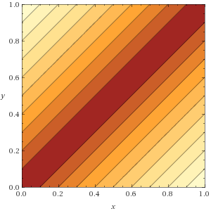
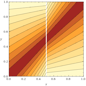
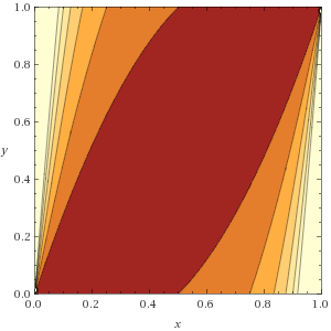
$\operatorname{AE}$                                  $\operatorname{NAE}$                                  $\operatorname{RAE}$

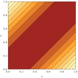
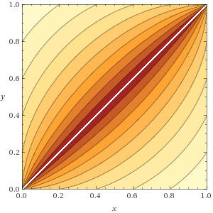
$\operatorname{NRAE}$                                  $\operatorname{SE}$                                  $\operatorname{DR}$

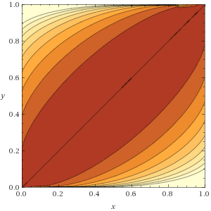
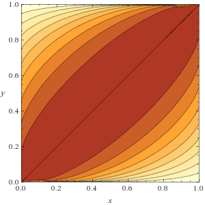
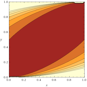
$\operatorname{KLD}$                                  $\operatorname{NKLD}$                                  $\operatorname{PD}$

Figure 1: 2D plots (for a binary quantification task) for the nine EMQs of Tables 1 and 2; $p(c_{1})$ and $p(c_{2})$ are represented as $x$ and $(1-x)$, respectively, while $\hat{p}(c_{1})$ and $\hat{p}(c_{2})$ are represented as $y$ and $(1-y)$. Darker areas represent values closer to 0 (i.e., smaller error) while lighter areas represent values more distant from 0 (i.e., higher error).

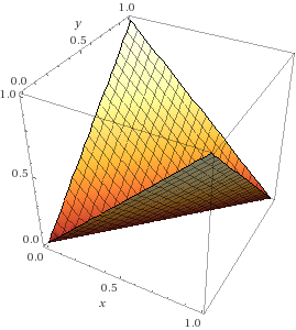
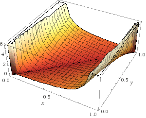
$\operatorname{AE}$                                  $\operatorname{NAE}$                                  $\operatorname{RAE}$

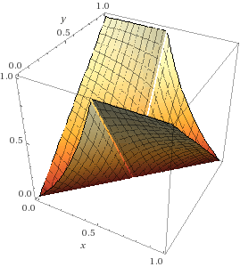
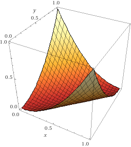
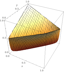
$\operatorname{NRAE}$                                  $\operatorname{SE}$                                  $\operatorname{DR}$

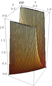
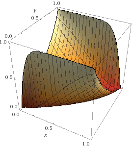
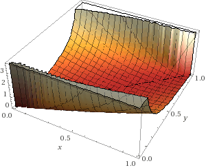
$\operatorname{KLD}$                                  $\operatorname{NKLD}$                                  $\operatorname{PD}$

Figure 2: 3D plots (for a binary quantification task) for the nine EMQs of Tables 1 and 2; $p(c_{1})$ and $p(c_{2})$ are represented as $x$ and $(1-x)$, respectively, while $\hat{p}(c_{1})$ and $\hat{p}(c_{2})$ are represented as $y$ and $(1-y)$; error is represented as $z$ (higher values of $z$ represent higher error).

It is easy to prove that $\operatorname{AE}$ enjoys IoI, NN, MON, IMP, ABS, IND. While some of these proofs are trivial, we report them in detail (in Appendix A) in order to show how the same arguments can be used to prove the same for many of the EMQs to be discussed later in this section.

Instead, as shown in Appendix B.1, $\operatorname{AE}$ does not enjoy MAX, because its range depends on the true distribution $p$. More specifically, $\operatorname{AE}$ ranges between 0 (best) and

$$z_{\operatorname{AE}}=\displaystyle\frac{2(1-\displaystyle\min_{c\in\mathcal{C}}p(c))}{|\mathcal{C}|}$$ (2)

(worst), i.e., its range depends also on the cardinality of $\mathcal{C}$. In fact, it is easy to verify that, given a true distribution $p$ on $\mathcal{C}$, the perverse estimator of $p$ is the one such that (a) $\hat{p}(c^{*})=1$ for class $c^{*}=\arg\min_{c\in\mathcal{C}}p(c)$, and (b) $\hat{p}(c)=0$ for all $c\in\mathcal{C}/\{c^{*}\}$. In this case, the total absolute error derives (i) from overestimating $p(c^{*})$, which brings about an error of $(1-p(c^{*}))$, and (ii) from underestimating $p(c)$ for all $c\in\mathcal{C}/\{c^{*}\}$, which collectively brings about an additional error of $(1-p(c^{*}))$. The mean absolute error is obtained by dividing this $2(1-p(c^{*}))$ quantity by $|\mathcal{C}|$.

Concerning REL, just note that since $\operatorname{AE}$ satisfies ABS, it cannot (as observed in Section 3) satisfy REL. (That $\operatorname{AE}$ does not enjoy REL is also shown via a counterexample in Appendix B.3.)

The properties that $\operatorname{AE}$ enjoys (and those it does not enjoy) are conveniently summarized in Table 1, along with the same for all the measures discussed in the rest of this paper.

In the literature, $\operatorname{AE}$ also goes by the name of Variational Distance (Csiszár and Shields, 2004, §4),(Lin, 1991; Zhang and Zhou, 2010), or Percentage Discrepancy (Esuli and Sebastiani, 2010; Baccianella et al., 2013). Also, if viewed as a generic function of dissimilarity between vectors (and not just probability distributions), $\operatorname{AE}$ is nothing else than the well-known “city-block distance” normalized by the number of classes. Some recent papers (Beijbom et al., 2015; González et al., 2017) that tackle quantification in the context of ecological modelling discuss or use, as an EMQ, Bray-Curtis dissimilarity (BCD), a measure popular in ecology for measuring the dissimilarity of two samples. However, when used to measure the dissimilarity of two probability distributions, BCD defaults to $\operatorname{AE}$; as a result we will not analyse BCD any further.

Note that $\operatorname{AE}$ often goes by the name of Mean Average Error; for simplicity, for this and the other measures we discuss in the rest of this paper we will omit the qualification “Mean”, since every measure mediates across the class-specific values in its own way.

As an EMQ, $\operatorname{AE}$ was used for the first time by (Saerens et al., 2002), and in many other papers ever since. For $\operatorname{AE}$ and for all the other EMQs discussed in this paper, Table 2 lists the papers where the measure has been proposed and those which have subsequently used it for evaluation purposes.

4.2 Normalized Absolute Error

Following what we have said in Section 4.1, a normalized version of $\operatorname{AE}$ that always ranges between 0 (best) and 1 (worst) can be obtained as

$$\operatorname{NAE}(p,\hat{p}) =\ \dfrac{\operatorname{AE}(p,\hat{p})}{z_{\operatorname{AE}}}=\ \frac{\sum_{c\in\mathcal{C}}|\hat{p}(c)-p(c)|}{2(1-\displaystyle\min_{c\in\mathcal{C}}p(c))}$$ (3)

where $z_{\operatorname{AE}}$ is as in Equation 2. It is easy to verify that $\operatorname{NAE}$ enjoys IoI, NN, MON, IMP, IND. $\operatorname{NAE}$ also enjoys (by construction) MAX.

Given that $\operatorname{NAE}$ is just a normalized version of $\operatorname{AE}$, and given that $\operatorname{AE}$ enjoys ABS, one might expect that $\operatorname{NAE}$ enjoys ABS too. Surprisingly enough, this is not the case, as shown in the counterexample of Appendix B.4. The reason for this is that, for the two distributions $p^{\prime}$ and $p^{\prime\prime}$ (and their respective predicted distributions $\hat{p}^{\prime}$ and $\hat{p}^{\prime\prime}$) mentioned in the formulation of Property 7 (ABS), and exemplified in the counterexample of Appendix B.4, the numerator of Equation 3 is the same but the denominator (i.e., the normalizing constant) is different, which means that the value of $\operatorname{NAE}$ is also different. $\operatorname{NAE}$ does not enjoy REL either, as also shown in Appendix B.3).

$\operatorname{NAE}$ was discussed for the first time by Esuli and Sebastiani (2014). With a similar intent, in a binary quantification context Barranquero et al. (2015) proposed Normalized Absolute Score ($\operatorname{NAS}$). $\operatorname{NAS}$ is an accuracy (and not an error) measure; when viewed as an error measure, it is defined as

$$\operatorname{NAS}(p,\hat{p})=\frac{|p(c)-\hat{p}(c)|}{\max\{p(c),(1-p(c))\}}$$ (4)

where $c$ is any class in $\mathcal{C}=\{c_{1},c_{2}\}$. We will not discuss $\operatorname{NAS}$ in detail since (a) it is only defined for the binary case, and (b) it is easy to show that in this case it coincides with $\operatorname{NAE}$.

4.3 Relative Absolute Error

Relative Absolute Error ($\operatorname{RAE}$) relativises the value $|\hat{p}(c)-p(c)|$ in Equation 1 to the true class prevalence, i.e.,

$$\operatorname{RAE}(p,\hat{p})=\frac{1}{|\mathcal{C}|}\sum_{c\in\mathcal{C}}\displaystyle\frac{|\hat{p}(c)-p(c)|}{p(c)}$$ (5)

$\operatorname{RAE}$ may be undefined in some cases, due to the presence of zero denominators. To solve this problem, in computing $\operatorname{RAE}$ we can smooth both $p(c)$ and $\hat{p}(c)$ via additive smoothing, i.e., we take

$$p_{s}(c)=\frac{\epsilon+p(c)}{\epsilon|\mathcal{C}|+\displaystyle\sum_{c\in\mathcal{C}}p(c)}$$ (6)

where $p_{s}(c)$ denotes the smoothed version of $p(c)$ and the denominator is just a normalizing factor (same for the $\hat{p}_{s}(c)$’s); the quantity $\epsilon=\frac{1}{2|\sigma|}$ is often used (and will always be used in the rest of this paper) as a smoothing factor. The smoothed versions of $p(c)$ and $\hat{p}(c)$ are then used in place of their original non-smoothed versions in Equation 5; as a result, $\operatorname{RAE}$ is always defined.

Using arguments analogous to the ones used for $\operatorname{AE}$ in Appendix A, it is immediate to show that $\operatorname{RAE}$ enjoys IoI, NN, MON, IMP, IND. It also enjoys REL by construction, which means that it does not enjoy ABS. Analogously to $\operatorname{AE}$, the fact $\operatorname{RAE}$ does not enjoy MAX, as shown via the counterexample in Appendix B.1.

It is easy to show that $\operatorname{RAE}$ ranges between 0 (best) and

$$z_{\operatorname{RAE}}=\displaystyle\frac{|\mathcal{C}|-1+\displaystyle\frac{1-\displaystyle\min_{c\in\mathcal{C}}p(c)}{\displaystyle\min_{c\in\mathcal{C}}p(c)}}{|\mathcal{C}|}$$ (7)

(worst), i.e., its range depends also on the cardinality of $\mathcal{C}$. In fact, similarly to the case of $\operatorname{AE}$, it is easy to verify that, given a true distribution $p$ on $\mathcal{C}$, the perverse estimator of $p$ is obtained when (a) $\hat{p}(c)=1$ for the class $c^{*}=\arg\min_{c\in\mathcal{C}}p(c)$, and (b) $\hat{p}(c)=0$ for all $c\in\mathcal{C}/\{c^{*}\}$. In this case, the total relative absolute error derives (i) from overestimating $p(c^{*})$, which brings about an error of $\frac{1-p(c^{*})}{p(c^{*})}$, and (ii) from underestimating $p(c)$ for all $c\in\mathcal{C}/\{c^{*}\}$, which brings about an additional error of 1 for each class in $\mathcal{C}/\{c^{*}\}$. The value of $\operatorname{RAE}$ is then obtained by dividing the resulting $(|\mathcal{C}|-1+\displaystyle\frac{1-p(c^{*})}{p(c^{*})})$ by $|\mathcal{C}|$.

As an EMQ, $\operatorname{RAE}$ was used for the first time by González-Castro et al. (2010), and by several other papers after it.

4.4 Normalized Relative Absolute Error

Following what we have said in Section 4.3, a normalized version of $\operatorname{RAE}$ that always ranges between 0 (best) and 1 (worst) can thus be obtained as

$$\operatorname{NRAE}(p,\hat{p})=\frac{\operatorname{RAE}(p,\hat{p})}{z_{\operatorname{RAE}}}=\frac{\displaystyle\sum_{c\in\mathcal{C}}\displaystyle\frac{|\hat{p}(c)-p(c)|}{p(c)}}{|\mathcal{C}|-1+\displaystyle\frac{1-\displaystyle\min_{c\in\mathcal{C}}p(c)}{\displaystyle\min_{c\in\mathcal{C}}p(c)}}$$ (8)

where $z_{\operatorname{RAE}}$ is as in Equation 7. Since the various denominators of Equation 8 may be undefined, the smoothed values of Equation 6 must be used in Equation 8 too.

It is straightforward to verify that $\operatorname{NRAE}$, which was first proposed by Esuli and Sebastiani (2014), enjoys IoI, NN, MON, IMP, IND, and also enjoys (by construction) MAX.

Somehow similarly to what we said in Section 4.2 about $\operatorname{NAE}$ and ABS, given that $\operatorname{NRAE}$ is just a normalized version of $\operatorname{RAE}$, and given that $\operatorname{RAE}$ enjoys REL, one might expect that $\operatorname{NRAE}$ enjoys REL too. Again, this is not the case, as shown in the counterexample of Appendix B.3. The reason for this is that, for the two distributions $p^{\prime}$ and $p^{\prime\prime}$ (and their respective predicted distributions $\hat{p}^{\prime}$ and $\hat{p}^{\prime\prime}$) mentioned in the formulation of Property 6 (REL), and exemplified in the counterexample of Appendix B.3, while $\operatorname{RAE}$ (the numerator of Equation 8) does enjoy REL, the normalizing constant (the denominator of Equation 8) invalidates it, since it is different for $p^{\prime}$ and $p^{\prime\prime}$. $\operatorname{NAE}$ does not enjoy ABS either, as also shown in Appendix B.4).

4.5 Squared Error

Another measure that has been used in the quantification literature is Squared Error ($\operatorname{SE}$), defined as

$$\operatorname{SE}(p,\hat{p})=\frac{1}{|\mathcal{C}|}\sum_{c\in\mathcal{C}}(p(c)-\hat{p}(c))^{2}$$ (9)

When viewed as a generic function of dissimilarity between vectors (and not just probability distributions), $\operatorname{SE}$ is the well-known $L^{2}$-distance. As an EMQ, $\operatorname{SE}$ was used for the first time by Bella et al. (2010).

The mathematical form of $\operatorname{SE}$ is very similar to that of $\operatorname{AE}$, and it can be trivially shown that $\operatorname{SE}$ enjoys all the properties that $\operatorname{AE}$ enjoys and does not enjoy all the properties that $\operatorname{AE}$ does not enjoy. In particular, $\operatorname{SE}$ does not enjoy MAX since $\operatorname{SE}$ ranges between 0 (best) and

$$z_{\operatorname{SE}}=\displaystyle\frac{(1-p(c^{*}))^{2}+\sum_{c\in\mathcal{C}/\{c^{*}\}}p(c)^{2}}{|\mathcal{C}|}$$ (10)

(worst), where $c^{*}=\arg\min_{c\in\mathcal{C}}p(c)$; i.e., the range of $\operatorname{SE}$ depends on $p$ and $|\mathcal{C}|$. In fact, similarly to the case of $\operatorname{AE}$, it is easy to verify that the perverse estimator of a true distribution $p$ is the one such (a) $\hat{p}(c^{*})=1$ and (b) $\hat{p}(c)=0$ for all $c\in\mathcal{C}/\{c^{*}\}$. In this case, the squared error derives (i) from overestimating $p(c^{*})$, which brings about an error of $\frac{(1-p(c^{*}))^{2}}{|\mathcal{C}|}$, and (ii) from underestimating $p(c)$ for all $c\in\mathcal{C}/\{c^{*}\}$, which brings about an additional error of $\frac{p(c)^{2}}{|\mathcal{C}|}$ for each class in $\mathcal{C}/\{c^{*}\}$. We could thus define a normalized version of $\operatorname{SE}$ as

$$\operatorname{NSE}(p,\hat{p})=\frac{\operatorname{SE}(p,\hat{p})}{z_{\operatorname{SE}}}=\frac{\sum_{c\in\mathcal{C}}(p(c)-\hat{p}(c))^{2}}{(1-p(c^{*}))^{2}+\sum_{c\in\mathcal{C}/\{c^{*}\}}p(c)^{2}}$$ (11)

which would, quite obviously, enjoy and not enjoy exactly the same properties that $\operatorname{NAE}$ enjoys and does not enjoy.

$\operatorname{SE}$ is structurally similar to $\operatorname{AE}$ but (as can also be appreciated from Figure 1) is less sensitive than it, i.e., it is always the case that $\operatorname{SE}(p,\hat{p})\leq\operatorname{AE}(p,\hat{p})$ (since it is always the case that $(p(c)-\hat{p}(c))^{2}\leq|p(c)-\hat{p}(c)|$).

In the binary quantification literature, other proxies of $\operatorname{SE}$ have been used; one example is Normalized Squared Score (Barranquero et al., 2015), defined as $\operatorname{NSS}(p(c),\hat{p}(c))\equiv 1-(\frac{p(c)-\hat{p}(c)}{\max\{p(c),(1-p(c))\}})^{2}$, where $c$ is any class in $\mathcal{C}=\{c_{1},c_{2}\}$. Similarly to the $\operatorname{NAS}$ measure discussed at the end of Section 4.1, NSS is an accuracy (and not an error) measure; when viewed as an error measure, it would be defined as

$$\operatorname{NSS}(p,\hat{p})=(\frac{p(c)-\hat{p}(c)}{\max\{p(c),(1-p(c))\}})^{2}$$ (12)

where $c$ is any class in $\mathcal{C}=\{c_{1},c_{2}\}$. We will not discuss $\operatorname{NSS}$ in detail since (a) it is only defined for the binary case, and (b) it is easy to show that in this case it coincides with $\operatorname{NSE}$.

4.6 Discordance Ratio

Levin and Roitman (2017) introduce an EMQ that they call Concordance Ratio (CR). $\operatorname{CR}$ is a measure of accuracy, and not a measure of error; for better consistency with the rest of this paper, instead of $\operatorname{CR}$ we consider what might be called Discordance Ratio, i.e., its complement $\operatorname{DR}=(1-\operatorname{CR})$, defined as

$$\operatorname{DR}(p,\hat{p})= \ 1-\operatorname{CR}$$ (13)

$$= \ 1-\frac{1}{|\mathcal{C}|}\sum_{c\in\mathcal{C}}\dfrac{\min\{(p(c),\hat{p}(c)\}}{\max\{(p(c),\hat{p}(c)\}}$$

$$= \ \frac{1}{|\mathcal{C}|}\sum_{c\in\mathcal{C}}\dfrac{\max\{(p(c),\hat{p}(c)\}-\min\{(p(c),\hat{p}(c)\}}{\max\{(p(c),\hat{p}(c)\}}$$

$$= \ \frac{1}{|\mathcal{C}|}\sum_{c\in\mathcal{C}}\dfrac{|(p(c)-\hat{p}(c)|}{\max\{(p(c),\hat{p}(c)\}}$$

$\operatorname{DR}$ is undefined when, for a given class $c$, both $p(c)$ and $\hat{p}(c)$ are zero; the smoothed values of Equation 6 must thus be used within Equation 13 in order to avoid this problem.

It is easy to verify, along the lines sketched in Appendix A, that $\operatorname{DR}$ enjoys IoI, NN, MON, IND. $\operatorname{DR}$ also enjoys REL; this can be seen by the fact that, for the same amount $a$ of misprediction, $\sum_{c\in\mathcal{C}}\frac{\min\{(p(c),\hat{p}(c)\}}{\max\{(p(c),\hat{p}(c)\}}$ is smaller (hence $\operatorname{DR}(p,\hat{p})$ is larger) when the true prevalence of the class $c_{1}$ mentioned in the formulation of Property 6 (REL) is smaller. Instead, $\operatorname{DR}$ enjoys neither MAX, nor IMP, nor ABS, as shown in Appendixes B.1, B.2 and B.4, respectively.

4.7 Kullback-Leibler Divergence

An EMQ that has become somehow standard in the evaluation of single-label (and, a fortiori, binary) quantification, is Kullback-Leibler Divergence ($\operatorname{KLD}$ – also called Information Divergence, or Relative Entropy) (Csiszár and Shields, 2004) and defined as

$$\operatorname{KLD}(p,\hat{p})=\sum_{c\in\mathcal{C}}p(c)\log\frac{p(c)}{\hat{p}(c)}$$ (14)

As an EMQ, $\operatorname{KLD}$ was used for the first time (under the name Normalized Cross-Entropy) by Forman (2005). It should also be noted that $\operatorname{KLD}$ has been adopted as the official evaluation measure of the only quantification-related shared task that has been organized so far, Subtask D “Tweet Quantification on a 2-point Scale” of SemEval-2016 and Semeval-2017 “Task 4: Sentiment Analysis in Twitter” (Nakov et al., 2016; Nakov et al., 2017).

$\operatorname{KLD}$ may be undefined in some cases. While the case in which $p(c)=0$ is not problematic (since continuity arguments indicate that $0\log\frac{0}{a}$ should be taken to be 0 for any $a\geq 0$), the case in which $\hat{p}(c)=0$ and $p(c)>0$ is indeed problematic, since $a\log\frac{a}{0}$ is undefined for $a>0$. To solve this problem, we smooth values in the same way as already described in Section 4.3; as a result, $\operatorname{KLD}$ is always defined.

That $\operatorname{KLD}$ enjoys IoI and NN is not immediately evident (since $p(c)\log\frac{p(c)}{\hat{p}(c)}$ is negative whenever $p(c)<\hat{p}(c)$), but has been proven before (Csiszár and Shields, 2004, p. 423). Indeed, $\operatorname{KLD}$ is a well-known member of the class of f-divergences (Ali and Silvey, 1966) (Csiszár and Shields, 2004, §4), a class of functions that measure the difference between two probability distributions, and that all enjoy IoI and NN.

The fact that $\operatorname{KLD}$ enjoys MON is also not self-evident, essentially for the same reasons for which it is not self-evident that it enjoys IoI and NN. The proof that $\operatorname{KLD}$ enjoys MON is given in Appendix C, where we use the fact that $\operatorname{KLD}$ enjoys IND (something which can be easily shown via the arguments used in Appendix A) and thus limit ourselves to proving that it enjoys B-MON.

The fact that $\operatorname{KLD}$ enjoys neither MAX, nor IMP, nor REL, nor ABS is shown in Appendixes B.1, B.2, B.3, B.4, respectively. Concerning MAX we note that, in theory, the upper bound of $\operatorname{KLD}$ is not finite, since Equation 14 has predicted probabilities, and not true probabilities, at the denominator. That is, by making a predicted probability $\hat{p}(c)$ infinitely small we can make $\operatorname{KLD}$ infinitely large. However, since we use smoothed values, the fact that both $p$ and $\hat{p}$ are lower-bounded by $\epsilon$, and not by 0, has the consequence that $\operatorname{KLD}$ has a finite upper bound. The perverse estimator for $\operatorname{KLD}$ is the one such (a) $\hat{p}(c^{*})=1$ and (b) $\hat{p}(c)=0$ for all $c\in\mathcal{C}/\{c^{*}\}$. The value of this estimator is

$$z_{\operatorname{KLD}}(p,\hat{p})=p_{s}(c^{*})\log\frac{p_{s}(c^{*})}{1-(|\mathcal{C}|-1)\cdot\epsilon}+\sum_{c\in\mathcal{C}/\{c^{*}\}}p_{s}(c)\log\frac{p_{s}(c)}{\epsilon}$$ (15)

which shows that the range of $\operatorname{KLD}$ depends on $p$, the cardinality of $\mathcal{C}$, and even on the value of $\epsilon$. This is a further proof that $\operatorname{KLD}$ does not enjoy MAX.

4.8 Normalized Kullback-Leibler Divergence

Given what we have said in Section 4.7, one might define a normalized version of $\operatorname{KLD}$ (i.e., one that also enjoys MAX) as $\frac{\operatorname{KLD}(p,\hat{p})}{z_{\operatorname{KLD}}(p,\hat{p})}$, where $z_{\operatorname{KLD}}(p,\hat{p})$ is as in Equation 15. Esuli and Sebastiani (2014) follow instead a different route, and define a normalized version of $\operatorname{KLD}$ by applying to it a logistic function, i.e.,

$$\operatorname{NKLD}(p,\hat{p}) =2\frac{e^{\operatorname{KLD}(p,\hat{p})}}{e^{\operatorname{KLD}(p,\hat{p})}+1}-1$$ (16)

Like other previously discussed measures, also $\operatorname{NKLD}$ may be undefined in some cases; therefore, also in computing $\operatorname{NKLD}$ we need to use the smoothed values of Equation 6 in place of the original $p(c)$’s and $\hat{p}(c)$’s.

$\operatorname{NKLD}$ enjoys some of our properties of interest for the simple reason that $\operatorname{KLD}$ enjoys them; it is easy to verify that this is the case of IoI and NN. $\operatorname{NKLD}$ also enjoys MON and IND; this descends from the fact that $\operatorname{NKLD}(d,d^{\prime})<\operatorname{NKLD}(d,d^{\prime\prime})$ if and only if $\operatorname{KLD}(d,d^{\prime})<\operatorname{KLD}(d,d^{\prime\prime})$ (this derives from the fact that the logistic function is a monotonic transformation) and from the fact that $\operatorname{KLD}$ enjoys MON and IND, respectively. Concerning MAX, $\operatorname{NKLD}$ enjoys it by construction, because when a predicted prevalence $\hat{p}(c)$ tends to 0 $\operatorname{KLD}$ tends to $+\infty$, and $\operatorname{NKLD}$ thus tends to 1.

The fact that $\operatorname{KLD}$ enjoys neither IMP, nor REL, nor ABS, is shown in Appendixes B.2, B.3, B.4, respectively.

4.9 Pearson Divergence

The last EMQ we discuss is the Pearson Divergence ($\operatorname{PD}$ – see (du Plessis and Sugiyama, 2012)), also called the $\chi^{2}$ Divergence (Liese and Vajda, 2006), and defined as

$$\operatorname{PD}(p,\hat{p})= \frac{1}{|\mathcal{C}|}\sum_{c\in\mathcal{C}}\frac{(p(c)-\hat{p}(c))^{2}}{\hat{p}(c)}$$ (17)

As an EMQ, $\operatorname{PD}$ has been first used by Ceron et al. (2016). $\operatorname{PD}$ is undefined when, for a given class $c$, $\hat{p}(c)$ is zero; the smoothed values of Equation 6 must thus be used within Equation 17 in order to avoid this problem.

The arguments already used for $\operatorname{AE}$ in Appendix A can be easily used to show that $\operatorname{PD}$ enjoys IoI, NN, and IND. That $\operatorname{PD}$ enjoys MON is instead not self-evident; the proof that it indeed does is reported in Appendix C.

That $\operatorname{PD}$ enjoys neither MAX, nor IMP, nor REL, nor ABS, is shown in Appendixes B.1, B.2, B.3, B.4, respectively. The fact that $\operatorname{PD}$ does not enjoy MAX can also be shown with arguments used for showing the same for $\operatorname{KLD}$; that is, when a predicted probability $\hat{p}(c)$ is very small, $\operatorname{PD}$ becomes very large. Thanks to the fact that we use smoothed values, though, $\hat{p}$ is lower-bounded by $\epsilon$, and $\operatorname{PD}$ has thus a finite upper bound. Like for other EMQs we have already discussed, the perverse estimator for $\operatorname{PD}$ is the one that attributes 1 to the probability of class $c^{*}=\arg\min_{c\in\mathcal{C}}p(c)$ and 0 to the other classes, and its value is thus

$$z_{\operatorname{PD}}(p,\hat{p})=\frac{1}{|\mathcal{C}|}(\frac{1-(|\mathcal{C}|-1)\cdot\epsilon-p_{s}(c^{*})}{1-(|\mathcal{C}|-1)\cdot\epsilon}+\sum_{c\in\mathcal{C}/\{c^{*}\}}\frac{(p(c)-\epsilon)^{2}}{\epsilon})$$ (18)

which shows that the range of $\operatorname{PD}$ depends on $p$, the cardinality of $\mathcal{C}$, and the value of $\epsilon$. This suffices to show that $\operatorname{PD}$ does not enjoy MAX.

5 Discussion

The properties that the EMQs of Section 4 enjoy and do not enjoy are conveniently summarized in Table 1. Table 2 lists instead the papers where the various EMQs have been proposed and the papers where they have subsequently been used for evaluation purposes.

Table 1: Properties of the EMQs discussed in this paper.

	IoI	NN	MAX	MON	IMP	REL	ABS	IND
$\operatorname{AE}$	Yes	Yes	No	Yes	Yes	No	Yes	Yes
$\operatorname{NAE}$	Yes	Yes	Yes	Yes	Yes	No	No	Yes
$\operatorname{RAE}$	Yes	Yes	No	Yes	Yes	Yes	No	Yes
$\operatorname{NRAE}$	Yes	Yes	Yes	Yes	Yes	No	No	Yes
$\operatorname{SE}$	Yes	Yes	No	Yes	Yes	No	Yes	Yes
$\operatorname{DR}$	Yes	Yes	No	Yes	No	Yes	No	Yes
$\operatorname{KLD}$	Yes	Yes	No	Yes	No	No	No	Yes
$\operatorname{NKLD}$	Yes	Yes	Yes	Yes	No	No	No	Yes
$\operatorname{PD}$	Yes	Yes	No	Yes	No	No	No	Yes

Table 2: Research works about quantification where the EMQs discussed in this paper have been first proposed ($\bigstar$) and later used (✓).

	$\operatorname{AE}$	$\operatorname{NAE}$	$\operatorname{RAE}$	$\operatorname{NRAE}$	$\operatorname{SE}$	$\operatorname{DR}$	$\operatorname{KLD}$	$\operatorname{NKLD}$00	$\operatorname{PD}$
(Saerens et al., 2002)	$\bigstar$
(Forman, 2005)	✓						$\bigstar$
(Forman, 2006)	✓						✓
(Forman, 2008)	✓						✓
(Tang et al., 2010)	✓						✓
(Bella et al., 2010)	✓				$\bigstar$
(González-Castro et al., 2010)	✓		$\bigstar$
(Zhang and Zhou, 2010)	✓
(Alaíz-Rodríguez et al., 2011)	✓		✓
(Milli et al., 2013)							✓
(Barranquero et al., 2013)	✓
(González-Castro et al., 2013)	✓		✓
(Esuli and Sebastiani, 2014)	✓	$\bigstar$	✓	$\bigstar$			✓	$\bigstar$
(du Plessis and Sugiyama, 2014)					✓
(Esuli and Sebastiani, 2015)			✓				✓
(Gao and Sebastiani, 2015)	✓	✓	✓	✓			✓	✓
(Barranquero et al., 2015)	✓						✓
(Beijbom et al., 2015)	✓
(Milli et al., 2015)							✓
(Gao and Sebastiani, 2016)	✓	✓	✓	✓			✓	✓
(Ceron et al., 2016)	✓								$\bigstar$
(González et al., 2017)	✓
(Kar et al., 2016)							✓
(Nakov et al., 2016)							✓
(du Plessis et al., 2017)					✓
(Levin and Roitman, 2017)						$\bigstar$
(Pérez-Gállego et al., 2017)	✓				✓
(Tasche, 2017)			✓
(Nakov et al., 2017)	✓		✓				✓
(Maletzke et al., 2017)	✓	✓		✓
(Esuli et al., 2018)	✓		✓				✓
(Card and Smith, 2018)	✓
(Moreira dos Reis et al., 2018)	✓			✓
(Fernandes Vaz et al., 2018)					✓
(Sanya et al., 2018)							✓
(Pérez-Gállego et al., 2019)	✓				✓

5.1 Are all our Properties Equally Important?

An examination of Table 1 allows us to make a number of general considerations. The first one is that some of our properties (namely: IoI, NN, MON, IND) are unproblematic, since all the EMQs proposed so far satisfy them, while other properties (namely: MAX, IMP, REL, ABS) are failed by several EMQs, including ones (e.g., $\operatorname{AE}$, $\operatorname{KLD}$) that are almost standard in the quantification literature. The second, related observation is that, if we agree on the fact that the eight properties we have discussed are desirable, a number of EMQs that have been proposed in the quantification literature emerge as severely inadequate, since they fail several among these properties; this is true even if we discount the fact that, as we have already observed, REL and ABS are mutually exclusive. The case of $\operatorname{KLD}$ (which fails on counts of MAX, IMP, REL, ABS) is of special significance, since $\operatorname{KLD}$ has almost become a standard in the evaluation of single-label (and binary) quantification (from Table 2 $\operatorname{KLD}$ emerges as the 2nd most frequently used EMQ, after $\operatorname{AE}$).

However, an even more compelling fact that emerges from Table 1 is that no EMQ among those proposed so far satisfies (even discounting the mutual exclusivity of REL and ABS) all the proposed properties. This suggests that more research is needed in order to identify, or synthesize, an EMQ more satisfactory than all the existing ones.

At the same time, in the absence of a truly satisfactory EMD, we think that it is important to analyse whether all of our properties are equally important, or if some of them is less important than others and can thus be “sacrificed”. Judging from Table 1, the key stumbling block seems to be the MAX property, since all the EMQs that satisfy MAX (namely: $\operatorname{NAE}$, $\operatorname{NRAE}$, $\operatorname{NKLD}$) satisfy neither REL nor ABS. This is undesirable since, as argued at the end of Section 3.1, some applications of quantification do require REL, while some other applications do require ABS (and we can think of no application that requires neither). Among the EMQs that satisfy ABS (and not REL), $\operatorname{AE}$ and $\operatorname{SE}$ satisfy all other properties but MAX, while among the ones that satisfy REL (and not ABS), also $\operatorname{RAE}$ satisfies all other properties but MAX.

In other words, if we stick to available EMQs, if we want ABS or REL we need to renounce to MAX, while if we want MAX we need to renounce to both ABS and REL. How relatively desirable are these three properties? We recall from Section 3.1 that

1. the argument in favour of REL is that it reflects the needs of applications in which an estimation error of a given absolute magnitude should be considered more serious if it affects a rarer class;

2. the argument in favour of ABS is that it reflects the needs of applications in which an estimation error of a given absolute magnitude has the same impact independently from the true prevalence of the affected class;

3. the main (although not the only) argument in favour of MAX is that, if an EMD does not satisfy it, the $n$ samples on which we may want to compare our quantification algorithms will each have a different weight on the final result.

The relative importance of these three arguments is probably a matter of opinion. However, it is our impression that Arguments 1 and 2 are more compelling than Argument 3, since 1 and 2 are really about how an evaluation measure reflects the needs of the application for which one performs a given task (quantification, in our case); if the corresponding properties are not satisfied, one may argue that the quantification accuracy (or error) being measured is only loosely related to what the user really wants. Argument 3, while important, “only” implies that, if MAX is not satisfied, some samples will weigh more than others on the final result; while undesirable, this does not affect the experimental comparison among different quantification systems, since each of them is affected by this disparity in the same way. So, if we accept the idea of “sacrificing” MAX in order to retain REL or ABS, Table 1 indicates that our measures of choice should be

• $\operatorname{AE}$ (or $\operatorname{SE}$, which is structurally similar), for those applications in which an estimation error of a given absolute magnitude should be considered more serious when the true prevalence of the affected class is lower; and

• $\operatorname{RAE}$, for those applications in which an estimation error of a given absolute magnitude has the same impact independently from the true prevalence of the affected class.

5.2 Properties that Escape Formalization

While all the above discussion on the properties of EMQs has been unashamedly formal, we should also remember that choosing an evaluation measure instead of another should also be guided by practical considerations, i.e., by properties of the measure that are not necessarily amenable to formalization. One such property is understandability, i.e., how simple and intuitive is the mathematical form of an evaluation measure. While such simplicity might not be a primary concern for the researcher, or the mathematician, it might be for the practitioner. For instance, a company that wants to sell a text analytics product to a customer might need to run experiments on the customer’s own data and explain the results to the customer; since customers might not be mathematically savvy, the fact that the measure chosen is easily understandable to people with a minimal mathematical background is important. On this account, measures such as $\operatorname{AE}$ and $\operatorname{RAE}$ certainly win over other measures such as $\operatorname{KLD}$ and $\operatorname{NKLD}$, which the average customer would find hardly intelligible.

Another property that is difficult to formalize is robustness to outliers. Many EMQs often take the form of an average $D(p,\hat{p})=\frac{1}{|\mathcal{C}|}\sum_{c\in\mathcal{C}}f(p(c),\hat{p}(c))$ across the classes in the codeframe. If $D(p,\hat{p})$ is not “robust to outliers”, it means that an extreme value $f(p(c^{\prime}),\hat{p}(c^{\prime}))$ that may occur for some $c^{\prime}\in\mathcal{C}$ dominates on all the other values $f(p(c),\hat{p}(c))$ for $c\in\mathcal{C}/\{c^{\prime}\}$, giving rise to a high value of $D(p,\hat{p})$ that is essentially due to $c^{\prime}$ only. As the name implies, “robustness to outliers” is usually considered a desirable property; however, in some contexts it might also viewed as undesirable (e.g., we might want to avoid quantification methods that generate blatant mistakes, so we might want a measure that penalizes the presence of even one of them). Aside from the fact that its desirability is questionable, it should also be mentioned that “robustness to outliers” comes in degrees. E.g., absolute error is more robust to outliers than squared error, but squared error is more robust to outliers than “cubic error”, etc.; and all of them are vastly more robust to outliers than $\operatorname{KLD}$ and $\operatorname{NKLD}$. Which among these enforces the “right” level of robustness to outliers? This shows that robustness to outliers, independently from its desirability, cannot be framed as a binary property (i.e., one that a measure either enjoys or not), and thus escapes the type of analysis that we have carried out in this paper.

Another property which is difficult to formalize has to do with the set of values which an EMQ ranges on when evaluating realistic quantification systems (i.e., systems that exhibit a quantification accuracy equal or superior to, say, that of a trivial “classify and count” approach using SVMs). For these systems, the actual values that an EMQ takes should occupy a fairly small subinterval of its entire range. The question is: how small? One particularly problematic EMQ, from this respect, is $\operatorname{KLD}$. While its range is $[0,z_{\operatorname{KLD}}]$, where $z_{\operatorname{KLD}}$ is as in Equation 15, realistic quantification systems generate very small $\operatorname{KLD}$ values, so small that they are sometimes difficult to make sense of. One result is that two genuine quantifiers that are being compared experimentally may easily obtain results several orders of magnitude away. Such differences in performance are difficult to grasp. We should add to this that, if one wants to average $\operatorname{KLD}$ results across a set of samples (on this see also Section 5.3), the average is completely dominated by the value with the highest order of magnitude, and the others have little or no impact. Unfortunately, switching from $\operatorname{KLD}$ to $\operatorname{NKLD}$ does not help much in this respect since, for realistic quantification systems, $\operatorname{NKLD}(p,\hat{p})\approx\frac{1}{2}\operatorname{KLD}(p,\hat{p})$. The reason is that $\operatorname{NKLD}$ is obtained by applying a sigmoidal function (namely, the logistic function) to $\operatorname{KLD}$, and the tangent to this sigmoid for $x=0$ is $y=\frac{1}{2}x$; since the values of $\operatorname{KLD}$ for realistic quantifiers are (as we have observed above) very close to 0, for these values the $\operatorname{NKLD}(p,\hat{p})$ curve is well approximated by $y=\frac{1}{2}\operatorname{KLD}(p,\hat{p})$. As an EMQ, $\operatorname{NKLD}$ thus de facto inherits most of the problems of $\operatorname{KLD}.$

All of the above points to the fact that choosing a good EMQ (and the same may well be true for tasks other than quantification) should also be based, aside from the formal properties that the EMQ enjoys, on criteria that either resist or completely escape formalization, such as understandability and ease of use.

5.3 Evaluating Quantification across Multiple Samples

On a different note, we also need to stress a key difference between measures of classification accuracy and measures of quantification accuracy (or error). The objects of classification are individual unlabelled items, and all measures of classification accuracy (e.g., $F_{1}$) are defined with respect to a test set of such objects. The objects of quantification, instead, are samples, and all the measures of quantification accuracy we have discussed in this paper are defined on a single such sample (i.e., they measure how well the true distribution of the classes across this individual sample is approximated by the predicted distribution of the classes across the same sample). Since every evaluation is worthless if carried out on a single object, it is clear that quantification systems need to be evaluated on sets of samples. This means that every measure that we have discussed needs first to be evaluated on each sample, and then its global score across the test set (i.e. the set of samples on which testing is carried out) needs to be computed. This global score may be computed via any measure of central tendency, e.g., via an average, or a median, or other (for instance, if $\operatorname{NAE}$ is used, we might in turn use Average $\operatorname{NAE}$ or Median $\operatorname{NAE}$, where averages and medians are computed across a set of samples). We do not take any specific stand for or against computing global scores via any specific measure of central tendency, since each of them may serve different but legitimate purposes.

6 Conclusions

We have presented a study that “evaluates evaluation”, in the tradition of the so-called “axiomatic” approach to the study of evaluation measures for information retrieval and related tasks. Our effort has targeted quantification, an important task at the crossroads of information retrieval, data mining, and machine learning, and has consisted of analysing previously proposed evaluation measures for quantification using the toolbox of the above-mentioned “axiomatic” approach. The work closest in spirit to the present one is our past work on the analysis of evaluation measures for classification (Sebastiani, 2015). However, quantification poses more difficult problems than classification, since evaluation measures for quantification are inherently nonlinear (i.e., quantification error cannot be expressed as a linear function of the labelling error made on individual items). This is unlike classification, for which linear measures (e.g., standard accuracy, or $K$ – see Sebastiani (2015)) are possible.

We have proposed eight properties that, as we have argued, are desirable for measures that attempt to evaluate quantification (two such properties are actually mutually exclusive, and are desirable each in a different class of applications of quantification). Our analysis has revealed that, unfortunately, no existing evaluation measure for quantification satisfies all of these properties. While this points to the fact that more research is needed to identify, or synthesize, a truly adequate such measure, this also means that, for the moment being, we have to evaluate the relative desirability of the properties that the existing measures do not satisfy. We have argued that some such properties are more important than others, and that as a result two measures (“Absolute Error” and “Relative Absolute Error”) stand out as the most satisfactory ones (interestingly enough, they are also the most time-honoured ones, and the mathematically simplest ones). As we have argued, the former is more adequate for application contexts in which an estimation error of a given absolute magnitude should be considered more serious if it affects a rare class, while the latter is more adequate for those applications in which an estimation error of a given absolute magnitude has the same impact independently from the true prevalence of the affected class.

Appendix A Properties of $\operatorname{AE}$

We here prove that $\operatorname{AE}$ enjoys IoI, NN, IND, MON, IMP, ABS. While some of these proofs are trivial, these are reported in detail in order to show how the same arguments can be used to prove the same for many of the other EMQs discussed in Section 4.

$\operatorname{AE}$ enjoys IoI. In fact, $\operatorname{AE}(p,\hat{p})=\frac{1}{|\mathcal{C}|}\sum_{c\in\mathcal{C}}|\hat{p}(c)-p(c)|=0$ implies that $\sum_{c\in\mathcal{C}}|\hat{p}(c)-p(c)|=0$; given that $\sum_{c\in\mathcal{C}}|\hat{p}(c)-p(c)|$ is a sum of nonnegative factors, this implies that $|\hat{p}(c)-p(c)|=0$ for all $c\in\mathcal{C}$, i.e., $\hat{p}(c)=p(c)$ for all $c\in\mathcal{C}$. Conversely, if $\hat{p}=p$, then $\frac{1}{|\mathcal{C}|}\sum_{c\in\mathcal{C}}|\hat{p}(c)-p(c)|=0$.          ∎

$\operatorname{AE}$ enjoys NN. Quite obviously, $\frac{1}{|\mathcal{C}|}\geq 0$ and $\sum_{c\in\mathcal{C}}|\hat{p}(c)-p(c)|\geq 0$, which implies that $\frac{1}{|\mathcal{C}|}\sum_{c\in\mathcal{C}}|\hat{p}(c)-p(c)|\geq 0$.          ∎

$\operatorname{AE}$ enjoys IND. Given codeframe $\mathcal{C}=\{c_{1},...,c_{k},c_{k+1},...,c_{n}\}$, for any true distribution $p$ on $\mathcal{C}$ and predicted distributions $\hat{p}^{\prime}$ and $\hat{p}^{\prime\prime}$ on $\mathcal{C}$ such that $\hat{p}^{\prime}(c)=\hat{p}^{\prime\prime}(c)$ for all $c\in\{c_{k+1},...,c_{n}\}$, the inequality

$$\operatorname{AE}(p,\hat{p}^{\prime})\leq\operatorname{AE}(p,\hat{p}^{\prime\prime})$$

resolves to

$$\frac{1}{|\mathcal{C}|}\sum_{c\in\mathcal{C}}|\hat{p}^{\prime}(c)-p(c)|\leq \ \frac{1}{|\mathcal{C}|}\sum_{c\in\mathcal{C}}|\hat{p}^{\prime\prime}(c)-p(c)|$$

$$\sum_{c\in\mathcal{C}}|\hat{p}^{\prime}(c)-p(c)|\leq \ \sum_{c\in\mathcal{C}}|\hat{p}^{\prime\prime}(c)-p(c)|$$

$$\sum_{c\in\mathcal{C}_{1}}|\hat{p}^{\prime}(c)-p(c)|+\sum_{c\in\mathcal{C}_{2}}|\hat{p}^{\prime}(c)-p(c)|\leq \ \sum_{c\in\mathcal{C}_{1}}|\hat{p}^{\prime\prime}(c)-p(c)|+\sum_{c\in\mathcal{C}_{2}}|\hat{p}^{\prime\prime}(c)-p(c)|$$

$$\sum_{c\in\mathcal{C}_{1}}|\hat{p}^{\prime}(c)-p(c)|\leq \ \sum_{c\in\mathcal{C}_{1}}|\hat{p}^{\prime\prime}(c)-p(c)|$$

$$\frac{1}{|\mathcal{C}_{1}|}\sum_{c\in\mathcal{C}_{1}}|\hat{p}^{\prime}(c)-p(c)|\leq \ \frac{1}{|\mathcal{C}_{1}|}\sum_{c\in\mathcal{C}_{1}}|\hat{p}^{\prime\prime}(c)-p(c)|$$

$$\operatorname{AE}(p_{\mathcal{C}_{1}},\hat{p}_{\mathcal{C}_{1}}^{\prime})\leq \ \operatorname{AE}(p_{\mathcal{C}_{1}},\hat{p}_{\mathcal{C}_{1}}^{\prime\prime})\hskip 30.00005pt\mbox{}\qed$$

$\operatorname{AE}$ enjoys MON. This can be proven by showing that $\operatorname{AE}$ enjoys B-MON, since we have proven that it enjoys IND. Given codeframe $\mathcal{C}=\{c_{1},c_{2}\}$ and true distribution $p$, if predicted distributions $\hat{p}^{\prime},\hat{p}^{\prime\prime}$ are such that $\hat{p}^{\prime\prime}(c_{1})<\hat{p}^{\prime}(c_{1})\leq p(c_{1})$, then it holds that

$$\operatorname{AE}(p,\hat{p}^{\prime})= \ \frac{1}{2}(|\hat{p}^{\prime}(c_{1})-p(c_{1})|+|\hat{p}^{\prime}(c_{2})-p(c_{2})|)$$

$$< \ \frac{1}{2}(|\hat{p}^{\prime\prime}(c_{1})-p(c_{1})|+|\hat{p}^{\prime\prime}(c_{2})-p(c_{2})|)$$

$$= \ \operatorname{AE}(p,\hat{p}^{\prime\prime})\hskip 30.00005pt\mbox{}\qed$$

$\operatorname{AE}$ enjoys IMP. This can be shown by showing that $\operatorname{AE}$ enjoys B-IMP, since we have proven that it enjoys IND. Given codeframe $\mathcal{C}=\{c_{1},c_{2}\}$, true distribution $p$, predicted distributions $\hat{p}^{\prime}$ and $\hat{p}^{\prime\prime}$, and constant $a\geq 0$ such that $\hat{p}^{\prime}(c_{1})=p(c_{1})+a$ and $\hat{p}^{\prime\prime}(c_{1})=p(c_{1})-a$, it holds that

$$\operatorname{AE}(p,\hat{p}^{\prime})= \ \frac{1}{2}(|\hat{p}^{\prime}(c_{1})-p(c_{1})|+|\hat{p}^{\prime}(c_{2})-p(c_{2})|)$$

$$= \ \frac{1}{2}(|(p(c_{1})+a)-p(c_{1})|+|(p(c_{2})-a)-p(c_{2})|)$$

$$= \ \frac{1}{2}(|a|+|-a|)$$

$$= \ \frac{1}{2}(|-a|+|a|)$$

$$= \ \frac{1}{2}(|(p(c_{1})-a)-p(c_{1})|+|(p(c_{2})+a)-p(c_{2})|)$$

$$= \ \operatorname{AE}(p,\hat{p}^{\prime\prime})\hskip 30.00005pt\mbox{}\qed$$

$\operatorname{AE}$ enjoys ABS. This can be shown by showing that $\operatorname{AE}$ enjoys B-ABS, since we have proven that it enjoys IND. Given codeframe $\mathcal{C}=\{c_{1},c_{2}\}$, constant $a>0$, true distributions $p^{\prime}$ and $p^{\prime\prime}$ such that $p^{\prime}(c_{1})<p^{\prime\prime}(c_{1})$ and $p^{\prime\prime}(c_{1})<p^{\prime\prime}(c_{2})$, if a predicted distribution $\hat{p}^{\prime}$ that estimates $p^{\prime}$ is such that $\hat{p}^{\prime}(c_{1})=p^{\prime}(c_{1})\pm a$ and a predicted distribution $\hat{p}^{\prime\prime}$ that estimates $p^{\prime\prime}$ is such that $\hat{p}^{\prime\prime}(c_{1})=p^{\prime\prime}(c_{1})\pm a$, then it holds that

$$\operatorname{AE}(p^{\prime},\hat{p}^{\prime})= \ \frac{1}{2}(|\hat{p}^{\prime}(c_{1})-p^{\prime}(c_{1})|+|\hat{p}^{\prime}(c_{2})-p^{\prime}(c_{2})|)$$

$$= \ \frac{1}{2}(|(p^{\prime}(c_{1})\pm a)-p^{\prime}(c_{1})|+|(p^{\prime}(c_{2})\mp a)-p^{\prime}(c_{2})|)$$

$$= \ \frac{1}{2}(2a)$$

$$= \ \frac{1}{2}((p^{\prime\prime}(c_{1})\pm a)-p^{\prime\prime}(c_{1})|+|(p^{\prime\prime}(c_{2})\mp a)-p^{\prime\prime}(c_{2})|)$$

$$= \ \frac{1}{2}(|\hat{p}^{\prime\prime}(c_{1})-p^{\prime\prime}(c_{1})|+|\hat{p}^{\prime\prime}(c_{2})-p^{\prime\prime}(c_{2})|)$$

$$= \ \operatorname{AE}(p^{\prime\prime},\hat{p}^{\prime\prime})\hskip 30.00005pt\mbox{}\qed$$

Appendix B Testing for MAX, IMP, ABS, REL

In this section we present simple tests aimed at establishing that a certain EMQ $D$ does not enjoy a certain property $\pi\in\{\textbf{MAX},\textbf{IMP},\textbf{ABS},\textbf{REL}\}$. The basic pattern of these tests is to show that $\pi$ does not hold for $D$ by providing a counterexample. More in particular, given a concrete scenario $s$ characterized by (1) a codeframe $\mathcal{C}$, (2) one or more true distributions $p_{1}$, $p_{2}$, …, and (3) one or more predicted distributions $\hat{p}_{1}$, $\hat{p}_{2}$, …, the test attempts to check whether the scenario satisfies the particular constraint that is required for property $\pi$ to hold. Since for $D$ to enjoy property $\pi$ the constraint is required to hold for all scenarios, if $\pi$ does not hold in $s$ we can conclude than $D$ does not enjoy $\pi$. Instead, if $\pi$ does hold in $s$ we can conclude nothing, and thus need to study the issue further.

B.1 A Counterexample for MAX

In the test for MAX we consider the scenario described in the following table

	$p(c_{1})$	$p(c_{2})$	$\hat{p}(c_{1})$	$\hat{p}(c_{2})$	$\operatorname{AE}$	$\operatorname{NAE}$	$\operatorname{RAE}$	$\operatorname{NRAE}$	$\operatorname{SE}$	$\operatorname{DR}$	$\operatorname{KLD}$	$\operatorname{NKLD}$	$\operatorname{PD}$
$p^{\prime}$	0.01	0.99	1.00	0.00	0.9900	1.0000	49.9975	1.0000	0.9801	0.9950	14.3076	0.9999	980100.0004
$p^{\prime\prime}$	0.49	0.51	1.00	0.00	0.5100	1.0000	41.0204	1.0000	0.2601	0.7550	16.7065	0.9975	260100.0001

and characterized by two different true distributions (1st and 2nd row) across the same codeframe $\mathcal{C}=\{c_{1},c_{2}\}$. The test consists in checking whether their respective perverse estimators obtain from $D$ the same score: if the values of measure $D$ in the two rows are not the same (greyed-out cells), this implies that $D$ does not satisfy MAX (if they are the same, this does not necessarily mean that $D$ satisfies MAX). Concerning the values obtained by $\operatorname{NKLD}$, see the discussion in Footnote 14.

The table shows that none of $\operatorname{AE}$, $\operatorname{RAE}$, $\operatorname{SE}$, $\operatorname{DR}$, $\operatorname{KLD}$, $\operatorname{PD}$ satisfies MAX.

B.2 A Counterexample for IMP

In the test for IMP we consider the scenario described in the following table

	$p(c_{1})$	$p(c_{2})$	$\hat{p}(c_{1})$	$\hat{p}(c_{2})$	$\operatorname{AE}$	$\operatorname{NAE}$	$\operatorname{RAE}$	$\operatorname{NRAE}$	$\operatorname{SE}$	$\operatorname{DR}$	$\operatorname{KLD}$	$\operatorname{NKLD}$	$\operatorname{PD}$
$p^{\prime}$	0.20	0.80	0.25	0.75	0.0500	0.0625	0.1562	0.0625	0.0025	0.1312	0.0070	0.0035	0.0117
$p^{\prime\prime}$	0.20	0.80	0.15	0.85	0.0500	0.0625	0.1562	0.0625	0.0025	0.1544	0.0090	0.0045	0.0181

and characterized by a codeframe $\mathcal{C}=\{c_{1},c_{2}\}$, a true distribution $p$ (Columns 2 and 3), and two predicted distributions $\hat{p}^{\prime}$ and $\hat{p}^{\prime\prime}$ (Columns 4 and 5, Rows 2 and 3) which are such that (i) $\hat{p}^{\prime}$ overestimates and $\hat{p}^{\prime\prime}$ underestimates the prevalence of a class $c_{1}$ by a certain amount $a>0$ (here: 0.05), and, symmetrically, (ii) $\hat{p}^{\prime}$ overestimates and $\hat{p}^{\prime\prime}$ underestimates the prevalence of another class $c_{2}$ by the same amount $a$. If the values of $D(p,\hat{p}^{\prime})$ and $D(p,\hat{p}^{\prime\prime})$ are not the same (which in the table is indicated by greyed-out cells), this implies that $D$ does not satisfy IMP (if they are the same, this does not necessarily mean that $D$ satisfies IMP).

The table shows that none of $\operatorname{DR}$, $\operatorname{KLD}$, $\operatorname{NKLD}$, $\operatorname{PD}$ satisfies IMP.

B.3 A Counterexample for REL

In the test for REL we consider the scenario described in the following table

	$p(c_{1})$	$p(c_{2})$	$\hat{p}(c_{1})$	$\hat{p}(c_{2})$	$\operatorname{AE}$	$\operatorname{NAE}$	$\operatorname{RAE}$	$\operatorname{NRAE}$	$\operatorname{SE}$	$\operatorname{DR}$	$\operatorname{KLD}$	$\operatorname{NKLD}$	$\operatorname{PD}$
$p^{\prime}$	0.20	0.80	0.70	0.30	0.5000	0.6250	1.5625	0.6250	0.2500	0.6696	0.5341	0.2609	0.7738
$p^{\prime\prime}$	0.25	0.75	0.75	0.25	0.5000	0.6667	1.3333	0.6667	0.2500	0.6667	0.5493	0.2679	0.8333

with a codeframe $\mathcal{C}=\{c_{1},c_{2}\}$, two true distributions $p^{\prime}$ and $p^{\prime\prime}$ (Rows 2 and 3, Columns 2 to 4), and two corresponding predicted distributions $\hat{p}^{\prime}$ and $\hat{p}^{\prime\prime}$ (Rows 2 and 3, Columns 5 to 7), such that in both cases the predicted distribution overestimates the prevalence of $c_{1}$ by the same amount $a>0$ (here: 0.50), with $p^{\prime}(c_{1})<p^{\prime\prime}(c_{1})$. Here, if it is not the case that $D(p,\hat{p}^{\prime})>D(p,\hat{p}^{\prime\prime})$ (which in the table is indicated by greyed-out cells), then $D$ does not satisfy REL (if $D(p,\hat{p}^{\prime})\not=D(p,\hat{p}^{\prime\prime})$, this does not necessarily mean that $D$ satisfies REL).

The table shows that none of $\operatorname{AE}$, $\operatorname{NAE}$, $\operatorname{NRAE}$, $\operatorname{SE}$, $\operatorname{KLD}$, $\operatorname{NKLD}$, $\operatorname{PD}$ satisfies REL.

B.4 A Counterexample for ABS

In the test for ABS we consider the same scenario as described in Appendix B.3, i.e.,

	$p(c_{1})$	$p(c_{2})$	$\hat{p}(c_{1})$	$\hat{p}(c_{2})$	$\operatorname{AE}$	$\operatorname{NAE}$	$\operatorname{RAE}$	$\operatorname{NRAE}$	$\operatorname{SE}$	$\operatorname{DR}$	$\operatorname{KLD}$	$\operatorname{NKLD}$	$\operatorname{PD}$
$p^{\prime}$	0.20	0.80	0.70	0.30	0.5000	0.6250	1.5625	0.6250	0.2500	0.6696	0.5341	0.2609	0.7738
$p^{\prime\prime}$	0.25	0.75	0.75	0.25	0.5000	0.6667	1.3333	0.6667	0.2500	0.6667	0.5493	0.2679	0.8333

with a codeframe $\mathcal{C}=\{c_{1},c_{2}\}$, two true distributions $p^{\prime}$ and $p^{\prime\prime}$ (Rows 2 and 3, Columns 2 to 4), and two corresponding predicted distributions $\hat{p}^{\prime}$ and $\hat{p}^{\prime\prime}$ (Rows 2 and 3, Columns 5 to 7), such that in both cases the predicted distribution overestimates the prevalence of $c_{1}$ by the same amount $a>0$ (here: 0.50), with $p^{\prime}(c_{1})<p^{\prime\prime}(c_{1})$. Here, if the values of $D(p,\hat{p}^{\prime})$ and $D(p,\hat{p}^{\prime\prime})$ are not equal (which in the table is indicated by greyed-out cells), this implies that $D$ does not satisfy ABS (if $D(p,\hat{p}^{\prime})=D(p,\hat{p}^{\prime\prime})$, this does not necessarily mean that $D$ satisfies ABS).

The table shows that none of $\operatorname{NAE}$, $\operatorname{RAE}$, $\operatorname{NRAE}$, $\operatorname{DR}$, $\operatorname{KLD}$, $\operatorname{NKLD}$, $\operatorname{PD}$ satisfies ABS.

Appendix C Proving that MON Holds

In this section we prove that MON holds for $\operatorname{KLD}$ and $\operatorname{PD}$. For this it will be sufficient to prove that $\operatorname{KLD}$ and $\operatorname{PD}$ enjoy B-MON, since it is immediate to verify that $\operatorname{KLD}$ and $\operatorname{PD}$ enjoy IND.

For ease of exposition, let us define the shorthands $a\equiv p(c_{1})$ and $x\equiv\hat{p}(c_{1})$. In order to show that $D$ satisfies B-MON it is sufficient to show that

1. if $(a-x)>0$, then $\dfrac{\partial}{\partial(a-x)}D>0$ for $a,x,(a-x)\in(0,1)$

2. if $(x-a)>0$, then $\dfrac{\partial}{\partial(x-a)}D>0$ for $a,x,(x-a)\in(0,1)$

because an increase in $(a-x)=(p(c_{1})-\hat{p}(c_{1}))$ implies an equivalent increase in $(p(c_{2})-\hat{p}(c_{2}))$ (same for $(x-a)$).

Theorem C.1

$\operatorname{KLD}$ satisfies B-MON.

Proof. We first treat the case $(a-x)>0$; let us define $y\equiv(a-x)$. In this case

$$\dfrac{\partial}{\partial y}\operatorname{KLD}= \ \dfrac{\partial}{\partial y}(a\log\dfrac{a}{x}+(1-a)\log\dfrac{1-a}{1-x})$$

$$= \ \dfrac{\partial}{\partial y}(a\log\dfrac{a}{a-y}+(1-a)\log\dfrac{1-a}{1-a+y})$$

$$= \ \dfrac{-y}{(a-y-1)(a-y)}$$

$$= \ \dfrac{x-a}{(x-1)x}$$

Since we are in the case in which $(x-a)<0$, and since $(x-1)<0$ and $x>0$, then $\dfrac{x-a}{(x-1)x}>0$ for all $a,x,(a-x)\in(0,1)$.

Let us now treat the case $(x-a)>0$, and let us define $y\equiv(x-a)$. In this case

$$\dfrac{\partial}{\partial y}\operatorname{KLD}= \ \dfrac{\partial}{\partial y}(a\log\dfrac{a}{x}+(1-a)\log\dfrac{1-a}{1-x})$$

$$= \ \dfrac{\partial}{\partial y}(a\log\dfrac{a}{y-a}+(1-a)\log\dfrac{1-a}{1-y+a})$$

$$= \ \dfrac{-y}{(a+y-1)(a+y)}$$

$$= \ \dfrac{a-x}{(x-1)x}$$

Since in this case it holds that $(a-x)<0$, and since $(x-1)<0$ and $x>0$, then $\dfrac{x-a}{(x-1)x}>0$ for all $a,x,(x-a)\in(0,1)$. This concludes our proof. ∎

Theorem C.2

$\operatorname{PD}$ satisfies B-MON.

Proof. We first treat the case $(a-x)>0$; let us define $y\equiv(a-x)$. In this case

$$\dfrac{\partial}{\partial y}\operatorname{PD}= \ \dfrac{\partial}{\partial y}(\dfrac{(a-x)^{2}}{x}+\dfrac{((1-a)-(1-x))^{2}}{1-x})$$

$$= \ \dfrac{\partial}{\partial y}(\dfrac{y^{2}}{a-y}+\dfrac{((1-a)-(1-a+y))^{2}}{1-a+y})$$

$$= \ \dfrac{y(-2a^{2}+2a(y+1)-y)}{(a-y)^{2}(-a+y+1)^{2}}$$

$$= \ \dfrac{(a-x)(a-2ax+x)}{x^{2}(1-x)^{2}}$$

Since in this case it holds that $a>x$, it is true that that $(a-2ax+x)>(x-2ax+x)=2x(1-a)>0$, since by hypothesis it holds that $x,a\in(0,1)$. Therefore, $\dfrac{\partial}{\partial y}\operatorname{PD}=\dfrac{(a-x)(a-2ax+x)}{x^{2}(1-x)^{2}}>0$, since the two factors at the numerator and the two factors at the denominator are all strictly $>0$.

Let us now treat the case $(x-a)>0$, and let us define $y\equiv(x-a)$. In this case

$$\dfrac{\partial}{\partial y}\operatorname{PD}= \ \dfrac{\partial}{\partial y}(\dfrac{(a-x)^{2}}{x}+\dfrac{((1-a)-(1-x))^{2}}{1-x})$$

$$= \ \dfrac{\partial(\dfrac{y^{2}}{y+a}+\dfrac{((1-a)-(1-a-y))^{2}}{1-a-y}}{\partial y})$$

$$= \ \dfrac{y(-2a^{2}-2a(y-1)+y)}{(a-y+1)^{2}(a+y)^{2}}$$

$$= \ \dfrac{(x-a)(-2ax+x+a)}{(2a-x+1)^{2}x^{2}}$$

Since in this case it holds that $x>a$, it is true that that $(-2ax+x+a)>(-2ax+2a)=2a(1-x)>0$, since by hypothesis it holds that $x,a\in(0,1)$. Therefore, $\dfrac{\partial\operatorname{PD}}{\partial y}=\dfrac{(x-a)(-2ax+x+a)}{(2a-x+1)^{2}x^{2}}>0$, since the two factors at the numerator and the two factors at the denominator are all strictly $>0$. This concludes our proof. ∎