Suboptimal Control of Dividends under Exponential Utility
Abstract
We consider an insurance company modelling its surplus process by a Brownian motion with drift. Our target is to maximise the expected exponential utility of discounted dividend payments, given that the dividend rates are bounded by some constant.
The utility function destroys the linearity and the time homogeneity of the considered problem. The value function depends not only on the surplus, but also on time. Numerical considerations suggest that the optimal strategy, if it exists, is of a barrier type with a non-linear barrier. In the related article [12], it has been observed that standard numerical methods break down in certain parameter cases and no close form solution has been found.
For these reasons, we offer a new method allowing to estimate the distance of an arbitrary smooth enough function to the value function. Applying this method, we investigate the goodness of the most obvious suboptimal strategies - payout on the maximal rate, and constant barrier strategies - by measuring the distance of its performance function to the value function.
Key words: suboptimal control, Hamilton–Jacobi–Bellman equation, dividend payouts, Brownian risk model, exponential utility function.
2010 Mathematical Subject Classification: Primary
93E20
Secondary 91B30, 60H30
1 Introduction
Dividend payments of companies is one of the most important factors for analytic investors when they have to decide whether they invest into the firm. Furthermore, dividends serve as a sort of litmus paper, indicating the financial health of the considered company. Indeed, the reputation, and consequently commercial success of a company with a long record of dividend payments would be negatively impacted in the case the company will drop the payments. On the other hand, new companies can additionally strengthen their position by declaring dividends. For the sake of fairness, it should be mentioned that there are also some serious arguments against dividend payouts, for example for tax reasons it might be advantageous to withhold dividend payments. A discussion of the pros and contras of dividends distribution is beyond the scope of the present manuscript. We refer to surveys on the topic by Avanzi [4] or Albrecher and Thonhauser [2].
Due to its importance, the value of expected discounted dividends has been for a long time, and still remains, one of the most popular risk measures in the actuarial literature. Lots of papers have been written on maximizing the dividend outcome in various models.
Gerber [11], Bühlmann [8], Azcue and Muler [5], Albrecher and Thonhauser [1] are just some of the results obtained since de Finetti’s path-breaking paper [9].
Shreve, Lehoczky and Gaver [17] considered the problem for a general diffusion process, where the drift and the volatility fulfil some special conditions.
Modelling the surplus process via a Brownian motion with drift, was considered by Asmussen and Taksar [3], who could find the optimal strategy to be a constant barrier.
All the papers mentioned above deal with linear dividend payments. Non-linear dividend payments are considered in Hubalek and Schachermayer [13]. They apply various utility functions to the dividend rates before accumulation. Their result differs a lot from the classical result described in Asmussen and Taksar [3]. An interesting question is to consider the expected “present utility” of the discounted dividend payments. It means the utility function will be applied on the value of the discounted dividend payments.
Modeling the surplus by a Brownian motion with drift, Grandits et. al applied in [12] an exponential utility function to the value of unrestricted discounted dividends. In other words, they considered the expected utility of the present value of dividends and not the expected discounted utility of the dividend rates. In that paper, the existence of the optimal strategy could not be shown. We will investigate the related problem where the dividend payments are restricted to a finite rate. Note that using a non-linear utility function increases the dimension of the problem. Therefore, as for now, tackling the problem via the Hamilton–Jacobi–Bellman approach in order to find an explicit solution seems to be an unsolvable task. Of course, one can prove the value function to be the unique viscosity solution to the corresponding Hamilton–Jacobi–Bellman equation and try to solve the problem numerically. However, if the maximal allowed dividend rate is quite big the standard numerical methods like finite differences and finite elements break down. We discuss this in Section 5.
In this paper, we offer a new approach. Instead of proving the value function to be the unique viscosity solution to the corresponding Hamilton–Jacobi–Bellman equation, we investigate the “goodness” of suboptimal strategies.
We simply choose an arbitrary control with an easy-to-calculate return function and compare its performance, or rather an approximation of its performance, against the unknown value function.
The method is based on sharp occupation bounds which we find by a method developed for sharp density bounds in Baños and Krühner [6]. This enables us to make an educated guess and to check if our pick is indeed almost as good as the optimal strategy.
This approach drastically differs from procedures usually used for calculation of the value function in two ways. First, unlike most numerical schemes there is no convergence to the value function, i.e. one only gets a bound for the performance of one given strategy but no straightforward procedure to get better strategies. Second, our criterion has almost no influence from the dimension of the problem and is consequently directly applicable in higher dimensions.
The paper is organised as follows. In the next section, we motivate the problem and derive some basic properties of the value function. In Section 3, we consider the case of the maximal constant dividend rate strategy, the properties of the corresponding return function and the goodness of this strategy (a bound for the distance of the return function to the unknown value function). Section 4 investigates the goodness of a constant barrier strategy. In Section 5, we consider examples illustrating the classical and the new approach. Finally, in the appendix we gather technical proofs and establish occupation bounds.
2 Motivation
We consider an insurance company whose surplus is modelled as a Brownian motion with drift
where on some filtered space where is assumed to be the right-continuous filtration generated by . is obviously a Markov-process and we denote by respectively the probability measure respectively expectation conditioned on , also we use the notation . Further, we assume that the company has to pay out dividends, characterized by a dividend rate. Denoting the dividend rate process by , we can write the ex-dividend surplus process as
In the present manuscript we allow only allow dividend rate processes which are progressively measurable and satisfy for some maximal rate at any time . We call these strategies admissible. Let , , be the underlying utility function and the ruin time corresponding to the strategy under the measure . Our objective is to maximize the expected exponential utility of the discounted dividend payments until ruin. Since we can start our observation in every time point , the target functional is given by
Here, we assume that the dividend payout up to equals , for a rigorous simplification confer [12] or simply note that with already paid dividends up to time we have
The corresponding value function is defined by
where the supremum is taken over all admissible strategies . Note that , because ruin will happen immediately due to the oscillation of Brownian motion, i.e. for any strategy under . The Hamilton–Jacobi–Bellman (HJB) equation corresponding to the problem can be found similar as in [12], for general explanations confer for instance [16]:
| (1) |
We like to stress at this point that we neither show that the value function solves the (HJB) in some sense, nor that a good enough solution is the value function. In fact, our approach of evaluating the goodness of a given strategy compared to the unknown optimal strategy does not assume any knowledge about the optimal strategy.
Assuming that the optimal strategy exists and that the value function does satisfy the HJB in a suitable sense, we have for the optimal dividend rates
-a.s. for any .
Remark 2.1
For every dividend strategy it holds:
We conclude
and is a bounded function. Consider now a constant strategy , i.e. we always pay on the rate . The ex-dividend process becomes a Brownian motion with drift and volatility . Define further
| (2) |
and let , i.e. is the ruin time under the strategy . Here and in the following we define
| (3) |
With help of change of measure technique, see for example [16, p. 216], we can calculate the return function of the constant strategy by using the power series representation of the exponential function:
| (4) |
It is obvious, that in the above power series and summation can be interchanged yielding . In particular, we can now conclude
uniformly in .
Next, we show that for some special values of the maximal rate with a positive probability the ex-dividend surplus process remains positive up to infinity.
Remark 2.2
Let be an admissible strategy, where is the process under the strategy . Let further be the process under the constant strategy , i.e. is a Brownian motion with drift and volatility . Then it is clear that
If then it holds, see for example [7, p. 223], .
Finally, we gather one structural property of the value function which, however, is not used later.
Proposition 2.3
The value function is Lipschitz-continuous, strictly increasing in and decreasing in .
Proof.
It is clear that is strictly increasing in .
Consider further with . Let and be an arbitrary admissible strategy. Let be the ruin time for the strategy which is constant zero.
Define
| (5) |
for any . Using , confer for instance [7, p. 295], it follows with :
| (6) |
– Let and be the ruin time for the strategy which is constant zero. Let be arbitrary, be an admissible strategy which is -optimal for the starting point , i.e. . Define further . Then for under because for under . Since fulfils for any , we have
The last inequality follows from monotony of and the fact that the -random time is less or equal than -a.s. Because was arbitrary and due to (6) we find
Consequently, is Lipschitz-continuous in the space variable with Lipschitz-constant at most .
– Next, we consider the properties of the value function concerning the time variable. Because , it is clear that is strictly decreasing in .
Let further , and be an admissible strategy. Then, the strategy with is admissible. Since, is concave we have
Building the supremum over all admissible strategies on the right side of the above inequality and using Remark 2.1, yields
and, consequently, is Lipschitz-continuous as a function of with constant . ∎
3 Payout on the Maximal Rate
3.1 Could it be optimal to pay on the maximal rate up to ruin?
At first, we investigate the constant strategy , i.e. the dividends will be paid out at the maximal rate until ruin. In this section we find exact conditions under which this strategy is optimal. We already know from (4) that the corresponding return function is given by
It is obvious that is increasing and concave in and decreasing in . For further considerations we will need the following remark.
Remark 3.1
Consider , defined in (2), as a function of .
Since
it is easy to see that and are increasing in . Also, we have
We conclude that .
Further, we put to record
Also, we have
Thus, at the function attains the value , at its minimum point we have
and, finally, for it holds, due to Item 2 above, that . Thus, for every the function has a unique zero at .
Further, it is easy to check that in summation and differentiation can be interchanged. Derivation with respect to yields
In order to answer the optimality question, we have to look at the function . For simplicity, we multiply the above expression by , substitute by and define
| (7) |
If on , then does solve the HJB equation and as we will see, it is the value function in that case.
Proposition 3.2
is the value function if and only if . In that case is a classical solution to the HJB equation (1) and an optimal strategy is constant .
Proof.
It is easy to check that solves the differential equation
We first assume that and show that is the value function. Then we have for any and, hence Remark 3.1 yields
This yields immediately for all :
Let now be an arbitrary admissible strategy, its ruin time and . Applying Ito’s formula yields -a.s.
Since is bounded, the stochastic integral above is a martingale with expectation zero. For the second integral one obtains using the differential equation for :
Building the expectations on the both sides and letting , we obtain by interchanging limit and expectation (due to the bounded convergence theorem):
Since and , the expectation above is non-positive, giving for all admissible strategies . Therefore, is the value function.
Assume now and we assume for contradiction that is the value function. Then we have . It means in particular, that the function is negative also for some . Consequently, does not solve the HJB equation (1). Moreover, is smooth enough and has bounded -derivative. Thus, classical verifaction results, cf. [10], yield that solves the HJB equation. A contradiction.
∎
In the following, we assume .
3.2 The goodness of the strategy .
We now provide an estimate on the goodness of the constant payout strategy which relies only on the performance of the chosen strategy and on deterministic constants. Recall from (2) and (5) that
Proposition 3.3
Let . Then we have
where
Proof.
We know that the return function . Let be an arbitrary admissible strategy. Then, using Ito’s formula for under :
Using the differential equation for , one obtains as in the last proof:
Building the -expectations, letting and rearranging the terms, one has
Our goal is to find a -independent estimate for the expectation on the rhs. above, in order to gain a bound for the difference . We have
where the last inequality follows from Theorem A.1. ∎
4 Goodness of Constant Barrier Strategies
Shreve et al. [17] and Asmussen and Taksar [3] considered the problem of dividend maximization for a surplus described by a Bownian motion with drift. The optimal strategy there turned out to be a barrier strategy with a constant barrier.
Let and be given by , i.e. is a barrier strategy with a constant barrier and ruin time . The corresponding return function fulfils due to the Markov-property of
Note that for every we have
It means, the moment generating function of is infinitely often differentiable and all moments of exist. We define
Then, for , , and for , , it holds:
| (8) | ||||
| (9) |
where, for the fourth equality, we developed the first exponential function in the expectation into its power series and used the Markov property to see that the -law given of equals the -law of .
In order to analyse the performance function of a barrier strategy we will develop the performance function into integer powers of with -dependent coefficients and truncate at some . This will result in an approximation for the performance function which is much easier to handle but this incurs an additional truncation error. Inspecting Equations (8), (9) motivates the approximations
for where . In order to achieve a fit we choose and
This leaves the choice for open which we now motivate by inspecting the dynamics equation for which should be:
with boundary condition for .
It is easy to verify that and . However, since solves the equation
we find that
We will treat the term as an error term and otherwise equate the two expressions above. This allows to define the remaining coefficients which are given by:
for and the last line also for .
The following lemma shows that solves “almost” the same equation as is thought to solve. Instead of being zero we see an error term which converges for time to infinity faster than .
Lemma 4.1
We have
for any where
Proof.
The claim follows by inserting the definitions of and . ∎
We define
for any . We now want to compare the approximate performance function for the barrier strategy with level to the unknown value function. We will employ the same method as in Section 3.2 and rely on the occupation bounds from Theorem A.1. We have in mind that . The three error terms appearing on the right-hand side of the following proposition are in this order the error for behaving suboptimal above the barrier, the error for behaving suboptimal below the barrier and the approximation error.
Proposition 4.2
Proof.
Observe that is analytic outside the barrier and on and the second space derivative is a bounded function. Thus, we can apply the change of variables formula, confer [14].
Choose an arbitrary strategy and denote its ruin time by .
Like before, applying Lemma 4.1, taking expectations and letting yields:
where we used that . Inserting the definition of , pulling out the sum and applying Theorem A.1 yields
Since was an arbitrary strategy and the right hand side does not depend on , the claim follows. ∎
Now we quantify the notion . Here, we see a single error term which corresponds to the approximation error (third summand) in Proposition 4.2.
Lemma 4.3
Let . Then we have
5 Examples
Here, we consider two examples. The first one will illustrate how the value function and the optimal strategy can be calculated using a straightforward approach under various unproven assumptions. In fact, we will assume (without proof) that the value function is smooth enough, the optimal strategy is of barrier type and that the barrier, the value function above the barrier and the value function below the barrier have suitable power series representations. In [12] has been observed that similar power series – if exist – have very large coefficients for certain parameter choices. This could mean that the power series doesn’t converge or that insufficient computing power was at hand.
In the second subsection, we will illustrate the new approach and calculate the distance of the performance function of a constant barrier strategy to the value function. The key advantages of this approach are that we do not rely on properties of the value function, nor do we need to know how it looks like. From a practical perspective, if the value function cannot be found, one should simply choose any strategy with an easy-to-calculate return function. Then, it is good to know how large the error to the optimal strategy is.
5.1 The straightforward approach
In this example we let , , and . We try to find the value function numerically. However, we do not know whether the assumptions which we will make do actually hold true for any possible parameters — or, even for the parameters we chose.
We conjecture and assume that the optimal strategy is of a barrier type where the barrier is given by a time-dependent curve, say ; the value function is assumed to be a function and we define

We assume that
for some coefficients. Note that we do not investigate the question whether the functions , and have a power series representation. We define further auxiliary coefficients and :
Since we assume that the value function is twice continuously differentiable with respect to we have
| (10) | |||


Note that (10) yields . Therefore, we can conclude . Thus, we can find the coefficients , and from the three equations (10). Note that using the general Leibniz rule, one gets
For we define the coefficients
Thus, we have
Equating coefficients yields
| (11) |
Note that Equations (11) specify , and in th step. The coefficients given above have a recursive structure. Due to this fact the numerical calculations turn out to be very time- and disk space-consuming. Numerical calculations show that the above procedure yields well-defined power series for relative small values of . However, for big the coefficients explode, which makes the calculations unstable and imprecise especially for close to zero.
5.2 The distance to the value function

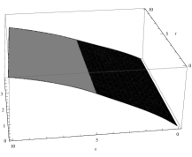
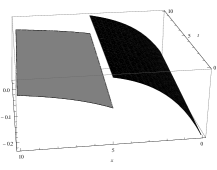
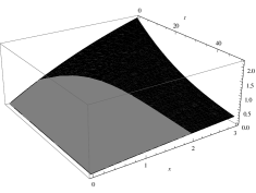
We use the same parameters as in the previous section, i.e. , , and . We illustrate the error bound given by Proposition 4.2 for summands and four different values for , namely , , and . We will compare the unknown value function to the performance of the barrier strategy with barrier at
i.e. we employ the strategy . This barrier strategy has been shown to be optimal if no utility function is applied, confer [16, p. 97]. In the case of one finds , i.e. we pay out at maximal rate all the time which is optimal due to Proposition 3.2. Therefore, this case is left with approximation error only. For the other values of , it is non-optimal to follow a barrier strategy and, hence, we do have a substantial error which cannot disappear in the limit. The corresponding pictures in Figure 5 show this error as for summands the approximation error is already several magnitudes smaller than the error incurred by following a suboptimal strategy.
Appendix A Appendix
In this section we provide deterministic upper bounds for the expected discounted occupation of a process whose drift is not precisely known. This allows to derive an upper bound for the expect discounted and cumulated positive functional of the process. These bounds are summarised in Theorem A.1.
Let with , , , , a standard Brownian motion and consider the process
where is some -valued progressively measurable process. We recall that we denote by a measure with . The local time of at level and time is denoted by and . Further we define for
Theorem A.1
We have . In particular, for any measurable function we have
The proof is given at the end of this section.
Lemma A.2
is absolutely continuous in its first variable with derivative
For any the function is of finite variation and
where denotes the Dirac-measure in . Moreover, if we denote by the second derivative of with respect to the first variable for , then we get
Proof.
Straightforward. ∎
Lemma A.3
Let and assume that . Then
Proof.
Ito Tanaka’s formula together with the occupation time formula yield
Using the product formula yields
Since is bounded we see that the second summand is a martingale. If , then we find that
If and , then -a.s. and boundedness of yields
If and , then takes values in and , thus boundedness of yields again
Thus, we find by monotone convergence
∎
Proof of Theorem A.1.
Fix . For any progressively measurable process with values in we define
where and denotes a continuous version of the local time of . Clearly, we have
Moreover, the previous two lemmas yield that with
is the optimally controlled process and we get . (The process exists because the corresponding SDE admits pathwise uniqueness, confer [15, Thm IX.3.5].) ∎
Appendix B Lower unbounded drift occupation bound
We will generalise the results from the previous section to the case where no lower bound on the drift is given, i.e. the drift is only assumed to be upper Lipschitz-continuous with some rate (which might be negative). The bounds are summarised in Theorem A.1. Let , , , a standard Brownian motion and consider the process
where is some -valued progressively measurable process satisfying for any . And again, we denote by a measure with . The local time of at level and time is denoted by and .
Further we define for
Theorem B.1
We have . In particular, for any measurable function we have
Proof.
The proof follows from Theorem A.1 by taking the limit . ∎
Acknowledgments
The research of the first author was funded by the Austrian Science Fund (FWF), Project number V 603-N35. The first author is currently on leave from the University of Liverpool and would like to thank the University of Liverpool for support and cooperation.
References
- [1] H. Albrecher and S. Thonhauser. Dividend maximization under consideration of the time value of ruin. Insurance Math. Econ, 41:163–184, 2007.
- [2] H. Albrecher and S. Thonhauser. Optimality results for dividend problems in insurance. Revista de la Real Academia de Ciencias Exactas, Físicas y Naturales. Serie A. Matemáticas. RACSAM, 103(2):295–320, 2009.
- [3] S. Asmussen and M. Taksar. Controlled diffusion models for optimal dividend pay-out. Insurance Math. Econ, 20:1–15, 1997.
- [4] B. Avanzi. Strategies for dividend distribution: A review. North American Actuarial Journal, 13:217–251, 2009.
- [5] P. Azcue and N. Muler. Optimal reinsurance and dividend distribution policies in the cramér–lundberg model. Math. Finance, 15:261–308, 2005.
- [6] D. Baños and P. Krühner. Optimal density bounds for marginals of Itô processes. Communications on Stochastic Analysis, 10:131–150, 2016.
- [7] A. N. Borodin and P. Salminen. Handbook of Brownian Motion – Facts and Formulae. Birkhäuser Verlag, Basel, 1998.
- [8] H. Bühlmann. Mathematical Methods in Risk Theory. Springer-Verlag, New York, 1970.
- [9] B. de Finetti. Su un’impostazione alternativa della teoria collettiva del rischio. Transactions of the XVth congress of actuaries., 2:433–443, 1957.
- [10] W. H. Fleming and H. M. Soner. Controlled Markov processes and viscosity solutions. Springer, New York, 1st edition, 1993.
- [11] H. U. Gerber. Entscheidungskriterien für den zusammengesetzten Poisson-prozess. Schweiz. Verein. Versicherungsmath. Mitt, 69:185–228, 1969.
- [12] P. Grandits, F. Hubalek, W. Schachermayer, and M. Zigo. Optimal expected exponential utility of dividend payments in Brownian risk model. Scandinavian Actuarial Journal, 2:73–107, 2007.
- [13] F. Hubalek and W. Schachermayer. Optimizing expected utility of dividend payments for a Brownian risk process and a peculiar nonlinear ode. Insurance Math. Econ, 34:193–225, 2004.
- [14] G. Peskir. A change-of-variable formula with local time on curves. J. Theor. Probab., 18:499–535, 2005.
- [15] D. Revuz and M. Yor. Continuous martingales and Brownian motion. Springer, Berlin Heidelber, 3rd edition, 2005.
- [16] H. Schmidli. Stochastic Control in Insurance. Springer, London, 2008.
- [17] S. E. Shreve, J. P. Lehoczky, and D. P. Gaver. Optimal consumption for general diffusions with absorbing and reflecting barriers. SIAM J. Control and Optimization, 22:55–75, 1984.