Numerical approximation of curve evolutions
in Riemannian manifolds

Abstract

We introduce variational approximations for curve evolutions in two-dimensional Riemannian manifolds that are conformally flat, i.e. conformally equivalent to the Euclidean space. Examples include the hyperbolic plane, the hyperbolic disk, the elliptic plane as well as any conformal parameterization of a two-dimensional surface in ${\mathbb{R}}^{d}$, $d\geq 3$. In these spaces we introduce stable numerical schemes for curvature flow and curve diffusion, and we also formulate a scheme for elastic flow. Variants of the schemes can also be applied to geometric evolution equations for axisymmetric hypersurfaces in ${\mathbb{R}}^{d}$. Some of the schemes have very good properties with respect to the distribution of mesh points, which is demonstrated with the help of several numerical computations.

Key words. Riemannian manifolds, curve evolution equations, curvature flow, curve diffusion, elastic flow, hyperbolic plane, hyperbolic disk, elliptic plane, geodesic curve evolutions, finite element approximation, equidistribution

AMS subject classifications. 65M60, 53C44, 53A30, 35K55

1 Introduction

The evolution of curves in a two-dimensional manifold driven by a velocity involving the (geodesic) curvature of the curve appears in many situations in geometry and in applications. Examples are curve straightening via the elastic energy or image processing on surfaces. The first mathematical results on such flows go back to the work of ?, who studied curvature flow in the Euclidean plane. Later evolutions in more complex ambient spaces have been studied, see e.g. ???. In the Euclidean case it can be shown that closed curves shrink to a point in finite time and they become more and more round as they do so, see ? and ?. In the case of a general ambient space the solution behaviour is more complex. For example, some solutions exist for arbitrary times and others can become unbounded in finite or infinite time, see e.g. ?.

Curvature flow is a second order flow. However, also fourth order flows are of interest. Here we mention the elastic (Willmore) flow of curves and curve diffusion, both of which are highly nonlinear. Elastic flow is the $L^{2}$–gradient flow of the elastic energy, and in the hyperbolic plane and on the sphere it was recently studied by ?? and ?, respectively. The curve diffusion flow, sometimes also called surface diffusion flow, is the $H^{-1}$–gradient flow for the length of the curve, and, like the elastic flow, it also features second derivatives of the curvature.

In this paper, we also want to study situations, in which a curve evolves in a two-dimensional manifold that is not necessarily embedded in ${\mathbb{R}}^{3}$. An important example is the hyperbolic plane $\mathbb{H}^{2}$, which due to Hilbert’s classical theorem cannot be embedded into ${\mathbb{R}}^{3}$, see ? and e.g. ?, §11.1. It will turn out that we can derive stable numerical schemes for curve evolutions in two-dimensional Riemannian manifolds that are conformally equivalent to the Euclidean space. This means that charts exist such that in the parameter domain the metric tensor is a possibly inhomogeneous scalar multiple of the classical Euclidean metric. This in particular implies that the chart is angle preserving, we refer to ? for more details.

The numerical approximation of the evolution of curves in an Euclidean ambient space is very well developed, with many papers on parametric as well as level set methods. We refer to ? for an overview. However, for more general ambient spaces only a few papers dealing with numerical methods exist. Some numerical work is devoted to the evolution of curves on two-dimensional surfaces in ${\mathbb{R}}^{3}$. We refer to ??? for methods using a parametric approach. Besides, also a level set setting is possible in order to numerically move curves that are constrained on surfaces, see ??.

The setting in this paper is as follows. Let $I={\mathbb{R}}/{\mathbb{Z}}$ be the periodic interval $[0,1]$ and let $\vec{x}:I\to{\mathbb{R}}^{2}$ be a parameterization of a closed curve $\Gamma\subset{\mathbb{R}}^{2}$. On assuming that

$$|\vec{x}_{\rho}|\geq c_{0}>0\qquad\forall\ \rho\in I\,,$$ (1.1)

we introduce the arclength $s$ of the curve, i.e. $\partial_{s}=|\vec{x}_{\rho}|^{-1}\,\partial_{\rho}$, and set

$$\vec{\tau}(\rho)=\vec{x}_{s}(\rho)=\frac{\vec{x}_{\rho}(\rho)}{|\vec{x}_{\rho}(\rho)|}\qquad\mbox{and}\qquad\vec{\nu}(\rho)=-[\vec{\tau}(\rho)]^{\perp}\,,$$ (1.2)

where $\cdot^{\perp}$ denotes a clockwise rotation by $\frac{\pi}{2}$.

On an open set $H\subset\mathbb{R}^{2}$ we define a metric tensor as

$$[(\vec{v},\vec{w})_{g}](\vec{z})=g(\vec{z})\,\vec{v}\,.\,\vec{w}\quad\forall\ \vec{v},\vec{w}\in{\mathbb{R}}^{2}\qquad\text{ for }\vec{z}\in H\,,$$ (1.3)

where $\vec{v}\,.\,\vec{w}=\vec{v}^{T}\,\vec{w}$ is the standard Euclidean inner product, and where $g:H\to{\mathbb{R}}_{>0}$ is a smooth positive weight function. This is the setting one obtains for a two-dimensional Riemannian manifold that is conformally equivalent to the Euclidean plane. In local coordinates the metric is precisely given by (1.3), see e.g. ???. Let us mention that a two-dimensional Riemannian manifold locally allows for a conformal chart, see e.g. ?, §5.10. Examples of such situations are the hyperbolic plane, the hyperbolic disc and the elliptic plane. Other examples are given by curves on two-dimensional surfaces in $\mathbb{R}^{d}$, $d\geq 3$, that can be conformally parameterized, such as spheres without pole(s), catenoids and torii. Coordinates $(x_{1},x_{2})\in H$ together with a metric $g$ as in (1.3) are called isothermal coordinates, i.e. in all situations considered in this paper we assume that we have isothermal coordinates. We refer to Section 2 and ?, 3.29 in §3D for more information.

For a time-dependent curve $\vec{x}$ the simplest curvature driven flow is given as

$$\mathcal{V}_{g}=\varkappa_{g}\,.$$ (1.4)

Here $\mathcal{V}_{g}=g^{\frac{1}{2}}(\vec{x})\,\vec{x}_{t}\,.\,\vec{\nu}$ is the normal velocity with respect to the metric (1.3), and

$$\varkappa_{g}=g^{-\frac{1}{2}}(\vec{x})\left[\varkappa-\tfrac{1}{2}\,\vec{\nu}\,.\,\nabla\,\ln g(\vec{x})\right]$$ (1.5)

is the curvature of the curve with respect to the metric $g$. The vector $\vec{\nu}$, defined in (1.2) is the classical Euclidean normal, and $\varkappa$ is the classical Euclidean curvature of the curve. It satisfies the property

$$\varkappa\,\vec{\nu}=\vec{\varkappa}=\vec{\tau}_{s}=\vec{x}_{ss}=\frac{1}{|\vec{x}_{\rho}|}\left[\frac{\vec{x}_{\rho}}{|\vec{x}_{\rho}|}\right]_{\rho},$$ (1.6)

see ?.

In the Euclidean case, i.e. in the case $g\equiv 1$, the right hand side in the curvature flow (1.4) is equal to $\varkappa$, and in particular the parameterization $\vec{x}$ only appears via $\vec{x}_{\rho}$, cf. (1.5), (1.6). This is crucial for stability proofs for numerical methods that have been introduced earlier, cf. ???. In the case of a general ambient space, additional nonlinearities involving the variable $\vec{x}$ itself appear in $\varkappa_{g}$, so that the variational structure of (1.6) is lost. This makes the design of stable schemes highly non-trivial. In fact, no such schemes appear in the literature so far. We will introduce stable fully discrete schemes with the help of a non-standard convex-concave splitting. In particular, the splitting has to be chosen in terms of $g^{\frac{1}{2}}$. With the help of the splitting, we propose in Section 3 a semi-implicit scheme for which stability can be shown.

The outline of this paper is as follows. In Section 2 we derive the governing equations for curvature flow, curve diffusion and elastic flow, provide weak formulations and relate the introduced flows to geometric evolution equations for axisymmetric hypersurfaces. In Section 3 we introduce finite element approximations and show existence and uniqueness as well as stability results. Section 4 is devoted to several numerical results, which demonstrate convergence rates as well as a qualitatively good mesh behaviour. In two appendices we derive exact solutions and derive the geodesic curve evolution equations for a conformal parameterization.

2 Mathematical formulations

It is the aim of this paper to introduce numerical schemes for the situation where a curve $\Gamma=\vec{x}(I)$ evolves in a two-dimensional Riemannian manifold that is conformally equivalent to the Euclidean space. Curvature flow is the $L^{2}$–gradient flow of the length functional and we first review how length is defined with respect to the metric $g$. The length induced by (1.3) is defined as

$$[|\vec{v}|_{g}](\vec{z})=\left([(\vec{v},\vec{v})_{g}](\vec{z})\right)^{\frac{1}{2}}=g^{\frac{1}{2}}(\vec{z})\,|\vec{v}|\quad\forall\ \vec{v}\in{\mathbb{R}}^{2}\qquad\text{ for }\vec{z}\in H\,.$$ (2.1)

The distance between two points $\vec{z}_{0}$, $\vec{z}_{1}$ in $H$ is defined as

$$\operatorname{dist}_{g}(\vec{z}_{0},\vec{z}_{1})=\inf\left\{\int_{0}^{1}[|\vec{\gamma}_{\rho}(\rho)|_{g}](\vec{\gamma}(\rho))\;{\rm d}\rho:\vec{\gamma}\in C^{1}([0,1],H)\,,\ \vec{\gamma}(0)=\vec{z}_{0}\,,\ \vec{\gamma}(1)=\vec{z}_{1}\right\}.$$ (2.2)

It can be shown that $(H,\operatorname{dist}_{g})$ is a metric space, see ?, §1.4.

On recalling (2.1), the total length of the closed curve $\Gamma\subset H$ is given by

$$L_{g}(\vec{x})=\int_{I}[|\vec{x}_{\rho}|_{g}](\vec{x})\;{\rm d}\rho=\int_{I}g^{\frac{1}{2}}(\vec{x})\,|\vec{x}_{\rho}|\;{\rm d}\rho\,.$$ (2.3)

If $\Gamma=\vec{x}(I)$ encloses a domain $\Omega\subset H$, with $\partial\Omega=\Gamma$, we define the total enclosed area as

$$A_{g}(\Omega)=\int_{\Omega}g(\vec{z})\;{\rm d}\vec{z}\,.$$ (2.4)

For later use we observe that if $\Gamma=\vec{x}(I)=\partial\Omega$ is parameterized clockwise, then $\vec{\nu}\circ\vec{x}^{-1}$, recall (1.2), denotes the outer normal to $\Omega$ on $\partial\Omega=\Gamma$. An anti-clockwise parameterization, on the other hand, yields that $\vec{\nu}\circ\vec{x}^{-1}$ is the inner normal.

We remark that if we take (1.3) with

$$g(\vec{z})=(\vec{z}\,.\,\vec{e}_{2})^{-2}\quad\text{ and }\quad H={\mathbb{H}}^{2}:=\{\vec{z}\in{\mathbb{R}}^{2}:\vec{z}\,.\,\vec{e}_{2}>0\}\,,$$ (2.5a)

then we obtain the Poincaré half-plane model which serves as a model for the hyperbolic plane. Clearly,

$$g(\vec{z})=1\quad\text{ and }\quad H={\mathbb{R}}^{2}$$ (2.5b)

simplifies to the standard Euclidean situation. In the context of the numerical approximation of geometric evolution equations for axisymmetric surfaces in $${\mathbb{R}}^{3}$$, in the recent papers ?? the authors considered gradient flows, and their numerical approximation, of the energy

$$A_{\mathcal{S}}(\vec{x})=2\,\pi\,\int_{I}\vec{x}\,.\,\vec{e}_{2}\,|\vec{x}_{\rho}|\;{\rm d}\rho\,.$$ (2.5c)

Here we note that as the authors in ?? considered surfaces that are rotationally symmetric with respect to the $$x_{2} \vec{e}_{2} \vec{e}_{1}$$–axis, they in fact considered (2.5c) with replaced by . We note that (2.3) collapses to (2.5c) for the choice

$$g(\vec{z})=4\,\pi^{2}\,(\vec{z}\,.\,\vec{e}_{2})^{2}\quad\text{ and }\quad H={\mathbb{H}}^{2}\,.$$ (2.5d)

We also consider more general variants of (2.5a), namely

$$g(\vec{z})=(\vec{z}\,.\,\vec{e}_{2})^{-2\,\mu}\,,\ \mu\in{\mathbb{R}}\,,\quad\text{ and }\quad H={\mathbb{H}}^{2}\,,$$ (2.5e)

so that (2.5a) corresponds to $\mu=1$, while formally (2.5b) corresponds to $\mu=0$. As the latter choice leads to a constant metric, a suitable translation of the initial data in the $\vec{e}_{2}$ direction will ensure that any evolution for (2.5b) is confined to ${\mathbb{H}}^{2}$, and so (2.5b) and (2.5e) with $\mu=0$ are equivalent. In addition, (2.5d), up to the constant factor $4\,\pi^{2}$, corresponds to $\mu=-1$. For the evolution equations we consider in this paper, the constant factor $4\,\pi^{2}$ will only affect the time scale of the evolutions.

We remark that for $\mu\not=1$ the metric space ${\mathbb{H}}^{2}$ with the metric (2.2) induced by (2.5e) is not complete. To see this, we observe that the distance (2.2) between $a\,\vec{e}_{2}$ and $b\,\vec{e}_{2}$, for $a<b$, is bounded from above by

$$\int_{a}^{b}u^{-\mu}\,{\rm d}u=(1-\mu)^{-1}\left(b^{1-\mu}-a^{1-\mu}\right).$$

Hence, in the case $\mu>1$, the distance converges to zero as $a,b\to\infty$, and so $(n\,\vec{e}_{2})_{n\in{\mathbb{N}}}$ is a Cauchy sequence without a limit in ${\mathbb{H}}^{2}$. In the case $\mu<1$ we can argue similarly for the Cauchy sequence $(n^{-1}\,\vec{e}_{2})_{n\in{\mathbb{N}}}$, as its limit $\vec{0}\not\in{\mathbb{H}}^{2}$. The Hopf–Rinow theorem, cf. ?, then implies that the metric space ${\mathbb{H}}^{2}$ with the metric induced by (2.5e) for $\mu\not=1$ is not geodesically complete. Of course, in the special case $\mu=0$ we can choose $H={\mathbb{R}}^{2}$ to obtain the complete Euclidean space, (2.5b).

Further examples are given by the family of metrics

$$g(\vec{z})=\frac{4}{(1-\alpha\,|\vec{z}|^{2})^{2}}\quad\text{ and }H=\begin{cases}{\mathbb{D}}_{\alpha}=\{\vec{z}\in{\mathbb{R}}^{2}:|\vec{z}|<\alpha^{-\frac{1}{2}}\}&\alpha>0\,,\\ {\mathbb{R}}^{2}&\alpha\leq 0\,.\end{cases}$$ (2.6)

see e.g. ?, Definition 4.4. We note that (2.6) with $\alpha=1$ gives a model for the hyperbolic disk, see also ?, Definition 2.7. The metric (2.6) with $\alpha=-1$, on the other hand, models the geometry of the elliptic plane. This is obtained by doing a stereographic projection of the sphere onto the plane, see (2.73), below, for more details.

We note that the sectional curvature of $g$, also called the Gaussian curvature of $g$, can be computed by

$$S_{0}(\vec{z})=-\frac{\Delta\,\ln g(\vec{z})}{2\,g(\vec{z})}\qquad\vec{z}\in H\,,$$ (2.7)

see e.g. ?, Definition 2.4. We observe that for (2.5e) it holds that

$$S_{0}(\vec{z})=-\mu\,(\vec{z}\,.\,\vec{e}_{2})^{2\,(\mu-1)}\qquad\vec{z}\in H\,,$$ (2.8)

while for (2.6) it holds that

$$S_{0}(\vec{z})=-\alpha\qquad\vec{z}\in H\,.$$ (2.9)

Of special interest are metrics with constant sectional curvature. For example, (2.5b) gives $S_{0}=0$, (2.5a), i.e. (2.5e) with $\mu=1$, gives $S_{0}=-1$, while (2.6) gives $S_{0}=-\alpha$ .

From now on we consider a family of curves $\Gamma(t)$, parameterized by $\vec{x}(\cdot,t):I\to H\subset{\mathbb{R}}^{2}$. It then holds that

$$\frac{\rm d}{{\rm d}t}\,L_{g}(\vec{x}(t))=\int_{I}\left[\nabla\,g^{\frac{1}{2}}(\vec{x})\,.\,\vec{x}_{t}+g^{\frac{1}{2}}(\vec{x})\,\frac{(\vec{x}_{t})_{\rho}\,.\,\vec{x}_{\rho}}{|\vec{x}_{\rho}|^{2}}\right]|\vec{x}_{\rho}|\;{\rm d}\rho\,.$$ (2.10)

Let

$$\partial_{s_{g}}=|\vec{x}_{\rho}|_{g}^{-1}\,\partial_{\rho}=g^{-\frac{1}{2}}(\vec{x})\,|\vec{x}_{\rho}|^{-1}\,\partial_{\rho}=g^{-\frac{1}{2}}(\vec{x})\,\partial_{s}\,.$$ (2.11)

We introduce

$$\vec{\nu}_{g}=g^{-\frac{1}{2}}(\vec{x})\,\vec{\nu}=-g^{-\frac{1}{2}}(\vec{x})\,\vec{x}_{s}^{\perp}=-\vec{x}_{s_{g}}^{\perp}\quad\text{and}\quad\vec{\tau}_{g}=\vec{x}_{s_{g}}\,,$$ (2.12)

so that $\vec{\tau}_{g}\,.\,\vec{\nu}_{g}=0$ and $|\vec{\tau}_{g}|_{g}^{2}=|\vec{\nu}_{g}|_{g}^{2}=(\vec{\nu}_{g},\vec{\nu}_{g})_{g}=g(\vec{x})\,\vec{\nu}_{g}\,.\,\vec{\nu}_{g}=1$, and let

$$\mathcal{V}_{g}=(\vec{x}_{t},\vec{\nu}_{g})_{g}=g^{\frac{1}{2}}(\vec{x})\,\vec{x}_{t}\,.\,\vec{\nu}=g^{\frac{1}{2}}(\vec{x})\,\mathcal{V}\,.$$ (2.13)

It follows from (1.6) that

$$\nabla\,g^{\frac{1}{2}}(\vec{x}) =[\vec{\nu}\,(\vec{\nu}\,.\,\nabla)+\vec{\tau}\,(\vec{\tau}\,.\,\nabla)]\,g^{\frac{1}{2}}(\vec{x})=\vec{\nu}\,(\vec{\nu}\,.\,\nabla)\,g^{\frac{1}{2}}(\vec{x})+\vec{\tau}\,\frac{1}{|\vec{x}_{\rho}|}\left[g^{\frac{1}{2}}(\vec{x})\right]_{\rho}$$

$$=\vec{\nu}\,(\vec{\nu}\,.\,\nabla)\,g^{\frac{1}{2}}(\vec{x})+\frac{1}{|\vec{x}_{\rho}|}\left[g^{\frac{1}{2}}(\vec{x})\,\frac{\vec{x}_{\rho}}{|\vec{x}_{\rho}|}\right]_{\rho}-g^{\frac{1}{2}}(\vec{x})\,\frac{1}{|\vec{x}_{\rho}|}\left[\frac{\vec{x}_{\rho}}{|\vec{x}_{\rho}|}\right]_{\rho}$$

$$=\vec{\nu}\,(\vec{\nu}\,.\,\nabla)\,g^{\frac{1}{2}}(\vec{x})+\frac{1}{|\vec{x}_{\rho}|}\left[g^{\frac{1}{2}}(\vec{x})\,\frac{\vec{x}_{\rho}}{|\vec{x}_{\rho}|}\right]_{\rho}-g^{\frac{1}{2}}(\vec{x})\,\varkappa\,\vec{\nu}\,.$$ (2.14)

Combining (2.10), (2.14) and (2.13) yields that

$$\frac{\rm d}{{\rm d}t}\,L_{g}(\vec{x}(t)) =\int_{I}\left(\nabla\,g^{\frac{1}{2}}(\vec{x})-\frac{1}{|\vec{x}_{\rho}|}\left[g^{\frac{1}{2}}(\vec{x})\,\frac{\vec{x}_{\rho}}{|\vec{x}_{\rho}|}\right]_{\rho}\right).\,\vec{x}_{t}\,|\vec{x}_{\rho}|\;{\rm d}\rho$$

$$=\int_{I}\left[\vec{\nu}\,.\,\nabla\,g^{\frac{1}{2}}(\vec{x})-g^{\frac{1}{2}}(\vec{x})\,\varkappa\right]\vec{\nu}\,.\,\vec{x}_{t}\,|\vec{x}_{\rho}|\;{\rm d}\rho$$

$$=\int_{I}\left[\vec{\nu}_{g}\,.\,\nabla\,g^{\frac{1}{2}}(\vec{x})-\varkappa\right]\mathcal{V}_{g}\,|\vec{x}_{\rho}|\;{\rm d}\rho$$

$$=-\int_{I}g^{-\frac{1}{2}}(\vec{x})\left[\varkappa-\vec{\nu}_{g}\,.\,\nabla\,g^{\frac{1}{2}}(\vec{x})\right]\mathcal{V}_{g}\,|\vec{x}_{\rho}|_{g}\;{\rm d}\rho$$

$$=-\int_{I}\varkappa_{g}\,\mathcal{V}_{g}\,|\vec{x}_{\rho}|_{g}\;{\rm d}\rho\,,$$ (2.15)

where, on recalling (2.12),

$$\varkappa_{g}=g^{-\frac{1}{2}}(\vec{x})\left[\varkappa-\vec{\nu}_{g}\,.\,\nabla\,g^{\frac{1}{2}}(\vec{x})\right]=g^{-\frac{1}{2}}(\vec{x})\left[\varkappa-\tfrac{1}{2}\,\vec{\nu}\,.\,\nabla\,\ln g(\vec{x})\right].$$ (2.16)

Clearly, the curvature $\varkappa_{g}$ is the first variation of the length (2.3).

For the metric (2.5e) we obtain that

$$\varkappa_{g}=(\vec{x}\,.\,\vec{e}_{2})^{\mu}\left[\varkappa+\mu\,\frac{\vec{\nu}\,.\,\vec{e}_{2}}{\vec{x}\,.\,\vec{e}_{2}}\right],$$ (2.17)

while for (2.6) we have

$$\varkappa_{g}=\tfrac{1}{2}\,(1-\alpha\,|\vec{x}|^{2})\left[\varkappa-2\,\alpha\,(1-\alpha\,|\vec{x}|^{2})^{-1}\,\vec{x}\,.\,\vec{\nu}\right].$$ (2.18)

In addition, combining (2.16), (2.12) and (2.14) yields that

$$g(\vec{x})\,\varkappa_{g}\,\vec{\nu}=\frac{1}{|\vec{x}_{\rho}|}\left[g^{\frac{1}{2}}(\vec{x})\,\frac{\vec{x}_{\rho}}{|\vec{x}_{\rho}|}\right]_{\rho}-\nabla\,g^{\frac{1}{2}}(\vec{x})\,.$$ (2.19)

Weak formulations of (1.6) and (2.19) will play an important role in this paper, and so we state them here for later reference. The natural weak formulation of (1.6) is

$$\int_{I}\varkappa\,\vec{\nu}\,.\,\vec{\eta}\,|\vec{x}_{\rho}|\;{\rm d}\rho+\int_{I}(\vec{x}_{\rho}\,.\,\vec{\eta}_{\rho})\,|\vec{x}_{\rho}|^{-1}\;{\rm d}\rho=0\quad\forall\ \vec{\eta}\in[H^{1}(I)]^{2}\,,$$ (2.20)

while a natural weak formulation of (2.19) is

$$\int_{I}g(\vec{x})\,\varkappa_{g}\,\vec{\nu}\,.\,\vec{\eta}\,|\vec{x}_{\rho}|\;{\rm d}\rho+\int_{I}\left[\nabla\,g^{\frac{1}{2}}(\vec{x})\,.\,\vec{\eta}+g^{\frac{1}{2}}(\vec{x})\,\frac{\vec{x}_{\rho}\,.\,\vec{\eta}_{\rho}}{|\vec{x}_{\rho}|^{2}}\right]|\vec{x}_{\rho}|\;{\rm d}\rho=0\quad\forall\ \vec{\eta}\in[H^{1}(I)]^{2}\,.$$ (2.21)

2.1 Curvature flow

It follows from (2.15) that

$$\mathcal{V}_{g}=\varkappa_{g}$$ (2.22)

is the natural $L^{2}$–gradient flow of $L_{g}$ with respect to the metric induced by $g$, i.e.

$$\frac{\rm d}{{\rm d}t}\,L_{g}(\vec{x}(t))+\int_{I}\varkappa_{g}^{2}\,|\vec{x}_{\rho}|_{g}\;{\rm d}\rho=0\,.$$ (2.23)

On recalling (2.13) and(2.16), we can rewrite (2.22) equivalently as

$$g(\vec{x})\,\vec{x}_{t}\,.\,\vec{\nu}=\varkappa-\tfrac{1}{2}\,\vec{\nu}\,.\,\nabla\,\ln g(\vec{x})\,.$$ (2.24)

We consider the following weak formulation of (2.24).
$(\mathcal{A})$: Let $\vec{x}(0)\in[H^{1}(I)]^{2}$. For $t\in(0,T]$ find $\vec{x}(t)\in[H^{1}(I)]^{2}$ and $\varkappa(t)\in L^{2}(I)$ such that (2.20) holds and

$$\int_{I}g(\vec{x})\,\vec{x}_{t}\,.\,\vec{\nu}\,\chi\,|\vec{x}_{\rho}|\;{\rm d}\rho=\int_{I}\left(\varkappa-\tfrac{1}{2}\,\vec{\nu}\,.\,\nabla\,\ln g(\vec{x})\right)\chi\,|\vec{x}_{\rho}|\;{\rm d}\rho\quad\forall\ i.e.\ \chi\in L^{2}(I)\,.$$ (2.25)

An alternative strong formulation of curvature flow to (2.24) is given by

$$g(\vec{x})\,\vec{x}_{t}=\vec{\varkappa}-\tfrac{1}{2}\,[\vec{\nu}\,.\,\nabla\,\ln g(\vec{x})]\,\vec{\nu}\,,$$ (2.26)

where we recall (1.6). We observe that (2.26) fixes $\vec{x}_{t}$ to be totally in the normal direction, in contrast to (2.24). We consider the following weak formulation of (2.26).
$(\mathcal{B})$: Let $\vec{x}(0)\in[H^{1}(I)]^{2}$. For $t\in(0,T]$ find $\vec{x}(t)\in[H^{1}(I)]^{2}$ and $\vec{\varkappa}(t)\in[L^{2}(I)]^{2}$ such that

$$\int_{I}g(\vec{x})\,\vec{x}_{t}\,.\,\vec{\chi}\,|\vec{x}_{\rho}|\;{\rm d}\rho=\int_{I}\left(\vec{\varkappa}\,.\,\vec{\chi}-\tfrac{1}{2}\,[\vec{\nu}\,.\,\nabla\,\ln g(\vec{x})]\,\vec{\nu}\,.\,\vec{\chi}\right)|\vec{x}_{\rho}|\;{\rm d}\rho\quad\forall\ \vec{\chi}\in[L^{2}(I)]^{2}\,,$$ (2.27a)

$$\int_{I}\vec{\varkappa}\,.\,\vec{\eta}\,|\vec{x}_{\rho}|\;{\rm d}\rho+\int_{I}(\vec{x}_{\rho}\,.\,\vec{\eta}_{\rho})\,|\vec{x}_{\rho}|^{-1}\;{\rm d}\rho=0\quad\forall\ \vec{\eta}\in[H^{1}(I)]^{2}\,.$$ (2.27b)

In order to develop stable approximations, we investigate alternative formulations based on (2.21). Firstly, we note that combining (2.24) and (2.16) yields

$$g(\vec{x})\,\vec{x}_{t}\,.\,\vec{\nu}=g^{\frac{1}{2}}(\vec{x})\,\varkappa_{g}\,.$$ (2.28)

We then consider the following weak formulation of (2.28).
$(\mathcal{C})$: Let $\vec{x}(0)\in[H^{1}(I)]^{2}$. For $t\in(0,T]$ find $\vec{x}(t)\in[H^{1}(I)]^{2}$ and $\varkappa_{g}(t)\in L^{2}(I)$ such that (2.21) holds and

$$\int_{I}g(\vec{x})\,\vec{x}_{t}\,.\,\vec{\nu}\,\chi\,|\vec{x}_{\rho}|\;{\rm d}\rho=\int_{I}g^{\frac{1}{2}}(\vec{x})\,\varkappa_{g}\,\chi\,|\vec{x}_{\rho}|\;{\rm d}\rho\quad\forall\ \chi\in L^{2}(I)\,.$$ (2.29)

Clearly, choosing $\chi=\varkappa_{g}$ in (2.29) and $\vec{\eta}=\vec{x}_{t}$ in (2.21) yields (2.23), on noting (2.13), (2.12) and (2.15).

On recalling (2.12), we introduce

$$\vec{\varkappa}_{g}=\varkappa_{g}\,\vec{\nu}_{g}=g^{-\frac{1}{2}}(\vec{x})\,\varkappa_{g}\,\vec{\nu}\,,$$ (2.30)

so that an alternative formulation of curvature flow to (2.22) is given by

$$\vec{x}_{t}=\mathcal{V}_{g}\,\vec{\nu}_{g}=\vec{\varkappa}_{g}\,,$$ (2.31)

where we have recalled (2.13) and (2.12). Similarly to (2.26), the flow (2.31) is again totally in the normal direction. On recalling (2.21) and (2.30), we consider the following weak formulation of (2.31).
$(\mathcal{D})$: Let $\vec{x}(0)\in[H^{1}(I)]^{2}$. For $t\in(0,T]$ find $\vec{x}(t)\in[H^{1}(I)]^{2}$ and $\vec{\varkappa}_{g}(t)\in[L^{2}(I)]^{2}$ such that

$$\int_{I}g(\vec{x})\,\vec{x}_{t}\,.\,\vec{\chi}\,|\vec{x}_{\rho}|\;{\rm d}\rho=\int_{I}g(\vec{x})\,\vec{\varkappa}_{g}\,.\,\vec{\chi}\,|\vec{x}_{\rho}|\;{\rm d}\rho\quad\forall\ \vec{\chi}\in[L^{2}(I)]^{2}\,,$$ (2.32a)

$$\int_{I}g^{\frac{3}{2}}(\vec{x})\,\vec{\varkappa}_{g}\,.\,\vec{\eta}\,|\vec{x}_{\rho}|\;{\rm d}\rho+\int_{I}\left[\nabla\,g^{\frac{1}{2}}(\vec{x})\,.\,\vec{\eta}+g^{\frac{1}{2}}(\vec{x})\,\frac{\vec{x}_{\rho}\,.\,\vec{\eta}_{\rho}}{|\vec{x}_{\rho}|^{2}}\right]|\vec{x}_{\rho}|\;{\rm d}\rho=0\quad\forall\ \vec{\eta}\in[H^{1}(I)]^{2}\,.$$ (2.32b)

Choosing $\vec{\chi}=g^{\frac{1}{2}}(\vec{x})\,\vec{\varkappa}_{g}$ in (2.32a) and $\vec{\eta}=\vec{x}_{t}$ in (2.32b) yields

$$\frac{\rm d}{{\rm d}t}\,L_{g}(\vec{x}(t))+\int_{I}g^{\frac{3}{2}}(\vec{x})\,|\vec{\varkappa}_{g}|^{2}\,|\vec{x}_{\rho}|\;{\rm d}\rho=0\,,$$ (2.33)

which is equivalent to (2.23), on recalling (2.15), (2.30) and (2.1).

We observe that the variable $\varkappa_{g}$ can be eliminated from $(\mathcal{C})$, by choosing $\chi=g^{\frac{1}{2}}(\vec{x})\,\vec{\nu}\,.\,\vec{\eta}$ in (2.29), and then combining (2.29) and (2.20), to yield

$$\int_{I}g^{\frac{3}{2}}(\vec{x})\,(\vec{x}_{t}\,.\,\vec{\nu})\,(\vec{\eta}\,.\,\vec{\nu})\,|\vec{x}_{\rho}|\;{\rm d}\rho+\int_{I}\left[\nabla\,g^{\frac{1}{2}}(\vec{x})\,.\,\vec{\eta}+g^{\frac{1}{2}}(\vec{x})\,\frac{\vec{x}_{\rho}\,.\,\vec{\eta}_{\rho}}{|\vec{x}_{\rho}|^{2}}\right]|\vec{x}_{\rho}|\;{\rm d}\rho=0$$

$$\hskip 312.9803pt\quad\forall\ \vec{\eta}\in[H^{1}(I)]^{2}\,.$$ (2.34)

Similarly, $\vec{\varkappa}_{g}$ can be eliminated from $(\mathcal{D})$ by choosing $\vec{\chi}=g^{\frac{1}{2}}(\vec{x})\,\vec{\eta}$ in (2.32a) to yield

$$\int_{I}g^{\frac{3}{2}}(\vec{x})\,\vec{x}_{t}\,.\,\vec{\eta}\,|\vec{x}_{\rho}|\;{\rm d}\rho+\int_{I}\left[\nabla\,g^{\frac{1}{2}}(\vec{x})\,.\,\vec{\eta}+g^{\frac{1}{2}}(\vec{x})\,\frac{\vec{x}_{\rho}\,.\,\vec{\eta}_{\rho}}{|\vec{x}_{\rho}|^{2}}\right]|\vec{x}_{\rho}|\;{\rm d}\rho=0\quad\forall\ \vec{\eta}\in[H^{1}(I)]^{2}\,.$$ (2.35)

2.2 Curve diffusion

We consider the flow

$$\mathcal{V}_{g}=-(\varkappa_{g})_{s_{g}s_{g}}=-g^{-\frac{1}{2}}(\vec{x})\left[g^{-\frac{1}{2}}(\vec{x})\left[\varkappa_{g}\right]_{s}\right]_{s}=-\frac{1}{g^{\frac{1}{2}}(\vec{x})\,|\vec{x}_{\rho}|}\left[\frac{[\varkappa_{g}]_{\rho}}{g^{\frac{1}{2}}(\vec{x})\,|\vec{x}_{\rho}|}\right]_{\rho}\,,$$ (2.36)

where we have recalled (2.11). On noting (2.15), and similarly to (2.23), it follows that (2.36) is the natural $H^{-1}$–gradient flow of $L_{g}$ with respect to the metric induced by $g$, i.e.

$$\frac{\rm d}{{\rm d}t}\,L_{g}(\vec{x}(t))+\int_{I}(\partial_{s_{g}}\,\varkappa_{g})^{2}\,|\vec{x}_{\rho}|_{g}\;{\rm d}\rho=0\,.$$ (2.37)

Moreover, if $\Gamma(t)=\vec{x}(I,t)$ encloses a domain $\Omega(t)\subset{\mathbb{R}}^{2}$, with $\vec{\nu}\circ\vec{x}^{-1}$ denoting the outer normal on $\partial\Omega(t)=\Gamma(t)$, on recalling (2.4), (2.1) and (2.13), it follows from a transport theorem, see e.g. ?, (2.22), that

$$\frac{\rm d}{{\rm d}t}\,A_{g}(\Omega(t))=\frac{\rm d}{{\rm d}t}\,\int_{\Omega(t)}g(\vec{z})\;{\rm d}\vec{z}=\int_{I}g(\vec{x})\,\mathcal{V}\,|\vec{x}_{\rho}|\;{\rm d}\rho=\int_{I}\mathcal{V}_{g}\,|\vec{x}_{\rho}|_{g}\;{\rm d}\rho\,.$$ (2.38)

Hence solutions to (2.36) satisfy, on noting (2.1), that

$$\frac{\rm d}{{\rm d}t}\,A_{g}(\Omega(t))=-\int_{I}(\varkappa_{g})_{s_{g}s_{g}}\,|\vec{x}_{\rho}|_{g}\;{\rm d}\rho=-\int_{I}\left[g^{-\frac{1}{2}}(\vec{x})\,[\varkappa_{g}]_{\rho}\right]_{\rho}\;{\rm d}\rho=0\,,$$ (2.39)

and so the total enclosed area is preserved.

Our weak formulations are going be to based on the equivalent equation

$$g(\vec{x})\,\vec{x}_{t}\,.\,\vec{\nu}=-\frac{1}{|\vec{x}_{\rho}|}\left(\frac{[\varkappa_{g}]_{\rho}}{g^{\frac{1}{2}}(\vec{x})\,|\vec{x}_{\rho}|}\right)_{\rho},$$ (2.40)

recall (2.13).

We consider the following weak formulation of (2.40), on recalling (2.16).
$(\mathcal{E})$: Let $\vec{x}(0)\in[H^{1}(I)]^{2}$. For $t\in(0,T]$ find $\vec{x}(t)\in[H^{1}(I)]^{2}$ and $\varkappa(t)\in H^{1}(I)$ such that (2.20) holds and

$$\int_{I}g(\vec{x})\,\vec{x}_{t}\,.\,\vec{\nu}\,\chi\,|\vec{x}_{\rho}|\;{\rm d}\rho=\int_{I}g^{-\frac{1}{2}}(\vec{x})\,\left(g^{-\frac{1}{2}}(\vec{x})\left[\varkappa-\tfrac{1}{2}\,\vec{\nu}\,.\,\nabla\,\ln g(\vec{x})\right]\right)_{\rho}\chi_{\rho}\,|\vec{x}_{\rho}|^{-1}\;{\rm d}\rho$$

$$\hskip 256.0748pt\quad\forall\ \chi\in H^{1}(I)\,.$$ (2.41)

We also introduce the following alternative weak formulation for (2.40), which treats the curvature $\varkappa_{g}$ as an unknown.
$(\mathcal{F})$: Let $\vec{x}(0)\in[H^{1}(I)]^{2}$. For $t\in(0,T]$ find $\vec{x}(t)\in[H^{1}(I)]^{2}$ and $\varkappa_{g}(t)\in H^{1}(I)$ such that (2.21) holds and

$$\int_{I}g(\vec{x})\,(\vec{x}_{t}\,.\,\vec{\nu})\,\chi\,|\vec{x}_{\rho}|\;{\rm d}\rho=\int_{I}g^{-\frac{1}{2}}(\vec{x})\,[\varkappa_{g}]_{\rho}\,\chi_{\rho}\,|\vec{x}_{\rho}|^{-1}\;{\rm d}\rho\quad\forall\ \chi\in H^{1}(I)\,.$$ (2.42)

Choosing $\chi=\varkappa_{g}$ in (2.42) and $\vec{\eta}=\vec{x}_{t}$ in (2.21) yields that (2.37) holds, on noting from (2.11) that

$$(\partial_{s_{g}}\,\varkappa_{g})^{2}\,|\vec{x}_{\rho}|_{g}=g^{-1}(\vec{x})\,|\vec{x}_{\rho}|^{-2}\,(\partial_{\rho}\,\varkappa_{g})^{2}\,g^{\frac{1}{2}}(\vec{x})\,|\vec{x}_{\rho}|=g^{-\frac{1}{2}}(\vec{x})\,(\partial_{\rho}\,\varkappa_{g})^{2}\,|\vec{x}_{\rho}|^{-1}\,.$$ (2.43)

2.3 Elastic flow

Here we consider an appropriate $L^{2}$–gradient flow of the elastic energy $W_{g}(\vec{x})$, where on recalling (2.30), (1.3), (2.16) and (2.1), we set

$$W_{g}(\vec{x}) =\tfrac{1}{2}\,\int_{I}|\vec{\varkappa}_{g}|_{g}^{2}\,|\vec{x}_{\rho}|_{g}\;{\rm d}\rho=\tfrac{1}{2}\,\int_{I}\varkappa_{g}^{2}\,|\vec{x}_{\rho}|_{g}\;{\rm d}\rho$$

$$=\tfrac{1}{2}\,\int_{I}g^{-\frac{1}{2}}(\vec{x})\left(\varkappa-\tfrac{1}{2}\,\vec{\nu}\,.\,\nabla\,\ln g(\vec{x})\right)^{2}|\vec{x}_{\rho}|\;{\rm d}\rho=\tfrac{1}{2}\,\int_{I}g^{-\frac{1}{2}}(\vec{x})\,\widetilde{\varkappa}_{g}^{2}\,|\vec{x}_{\rho}|\;{\rm d}\rho\,.$$ (2.44)

In the above, on recalling (2.16), we have defined

$$\widetilde{\varkappa}_{g}=g^{\frac{1}{2}}(\vec{x})\,\varkappa_{g}=\varkappa-{\mathfrak{z}}\,,\quad\text{with}\quad{\mathfrak{z}}=\vec{\nu}_{g}\,.\,\nabla\,g^{\frac{1}{2}}(\vec{x})=\tfrac{1}{2}\,\vec{\nu}\,.\,\nabla\,\ln g(\vec{x})\,.$$ (2.45)

In the following we often omit the dependence of $g$ on $\vec{x}$, and we simply write $g$ for $g(\vec{x})$ and so on. It follows from (2.3), (2.45), (2.13) and (2.1) that

$$\frac{\rm d}{{\rm d}t}\,W_{g}(\vec{x}(t))$$

$$\quad=\tfrac{1}{2}\,\int_{I}(g^{-\frac{1}{2}})_{t}\,\widetilde{\varkappa}_{g}^{2}\,|\vec{x}_{\rho}|\;{\rm d}\rho+\int_{I}g^{-\frac{1}{2}}\,(\widetilde{\varkappa}_{g})_{t}\,\widetilde{\varkappa}_{g}\,|\vec{x}_{\rho}|\;{\rm d}\rho+\tfrac{1}{2}\,\int_{I}g^{-\frac{1}{2}}\,\widetilde{\varkappa}_{g}^{2}\,\vec{x}_{\rho}\,.\,(\vec{x}_{t})_{\rho}\,|\vec{x}_{\rho}|^{-1}\;{\rm d}\rho$$

$$\quad=\tfrac{1}{2}\,\int_{I}(\vec{x}_{t}\,.\,\nabla\,g^{-\frac{1}{2}})\,\widetilde{\varkappa}_{g}^{2}\,|\vec{x}_{\rho}|\;{\rm d}\rho+\int_{I}g^{-\frac{1}{2}}\,(\widetilde{\varkappa}_{g})_{t}\,\widetilde{\varkappa}_{g}\,|\vec{x}_{\rho}|\;{\rm d}\rho-\tfrac{1}{2}\,\int_{I}(g^{-\frac{1}{2}}\,\widetilde{\varkappa}_{g}^{2}\,\vec{x}_{s})_{s}\,.\,\vec{x}_{t}\,|\vec{x}_{\rho}|\;{\rm d}\rho$$

$$\quad=\tfrac{1}{2}\,\int_{I}(\vec{x}_{t}\,.\,\nabla\,g^{-\frac{1}{2}})\,\widetilde{\varkappa}_{g}^{2}\,|\vec{x}_{\rho}|\;{\rm d}\rho+\int_{I}g^{-\frac{1}{2}}\,(\widetilde{\varkappa}_{g})_{t}\,\widetilde{\varkappa}_{g}\,|\vec{x}_{\rho}|\;{\rm d}\rho$$

$$\qquad\quad-\tfrac{1}{2}\,\int_{I}\left[(\vec{x}_{s}\,.\,\nabla\,g^{-\frac{1}{2}})\,\widetilde{\varkappa}_{g}^{2}\,\vec{x}_{s}+2\,g^{-\frac{1}{2}}\,\widetilde{\varkappa}_{g}\,(\widetilde{\varkappa}_{g})_{s}\,\vec{x}_{s}+g^{-\frac{1}{2}}\,\widetilde{\varkappa}_{g}^{2}\,\varkappa\,\vec{\nu}\right].\,\vec{x}_{t}\,|\vec{x}_{\rho}|\;{\rm d}\rho\,.$$

$$\quad=\tfrac{1}{2}\,\int_{I}(\vec{\nu}\,.\,\nabla\,g^{-\frac{1}{2}})\,\widetilde{\varkappa}_{g}^{2}\,\mathcal{V}\,|\vec{x}_{\rho}|\;{\rm d}\rho+\int_{I}g^{-\frac{1}{2}}\,\widetilde{\varkappa}_{g}\,[(\widetilde{\varkappa}_{g})_{t}-\,(\widetilde{\varkappa}_{g})_{s}\,\vec{x}_{s}\,.\,\vec{x}_{t}]\,|\vec{x}_{\rho}|\;{\rm d}\rho$$

$$\qquad\quad-\tfrac{1}{2}\,\int_{I}g^{-\frac{1}{2}}\,\widetilde{\varkappa}_{g}^{2}\,\varkappa\,\mathcal{V}\,|\vec{x}_{\rho}|\;{\rm d}\rho$$

$$\quad=\tfrac{1}{2}\,\int_{I}\left[(\vec{\nu}\,.\,\nabla\,g^{-\frac{1}{2}})-g^{-\frac{1}{2}}\,\varkappa\right]\varkappa_{g}^{2}\,\mathcal{V}_{g}\,|\vec{x}_{\rho}|_{g}\;{\rm d}\rho+\int_{I}\varkappa_{g}\,[(\widetilde{\varkappa}_{g})_{t}-\,(\widetilde{\varkappa}_{g})_{s}\,\vec{x}_{s}\,.\,\vec{x}_{t}]\,|\vec{x}_{\rho}|\;{\rm d}\rho\,.$$ (2.46)

We have from (2.45) that

$$\varkappa_{g}-g^{-\frac{1}{2}}\,\varkappa=-\tfrac{1}{2}\,g^{-\frac{1}{2}}\,\vec{\nu}\,.\,\nabla\,\ln g=\vec{\nu}\,.\,\nabla\,g^{-\frac{1}{2}}\,,$$ (2.47)

and so it follows from (2.46) that

$$\frac{\rm d}{{\rm d}t}\,W_{g}(\vec{x}(t)) =\tfrac{1}{2}\,\int_{I}\left[\varkappa_{g}-2\,g^{-\frac{1}{2}}\,\varkappa\right]\varkappa_{g}^{2}\,\mathcal{V}_{g}\,|\vec{x}_{\rho}|_{g}\;{\rm d}\rho+\int_{I}\varkappa_{g}\,[(\widetilde{\varkappa}_{g})_{t}-\,(\widetilde{\varkappa}_{g})_{s}\,\vec{x}_{s}\,.\,\vec{x}_{t}]\,|\vec{x}_{\rho}|\;{\rm d}\rho\,.$$ (2.48)

In order to deal with the last integral in (2.48), we observe the following. It follows from (1.2), (1.6) and (2.13) that

$$\vec{\nu}_{s} =-\varkappa\,\vec{x}_{s}\,,\quad\vec{\nu}_{ss}=-\varkappa_{s}\,\vec{x}_{s}-\varkappa^{2}\,\vec{\nu}\,,$$ (2.49a)

$$\vec{\nu}_{t} =-((\vec{x}_{s})_{t}\,.\,\vec{\nu})\,\vec{x}_{s}=-((\vec{x}_{\rho}\,|\vec{x}_{\rho}|^{-1})_{t}\,.\,\vec{\nu})\,\vec{x}_{s}=-((\vec{x}_{t})_{s}\,.\,\vec{\nu})\,\vec{x}_{s}\,,$$ (2.49b)

$$\vec{\nu}_{t}-(\vec{x}_{s}\,.\,\vec{x}_{t})\,\vec{\nu}_{s} =-\mathcal{V}_{s}\,\vec{x}_{s}\,.$$ (2.49c)

Combining (2.49a,b) yields, on recalling (2.13), that

$$\varkappa_{t} =-(\vec{x}_{s})_{t}\,.\,\vec{\nu}_{s}-\vec{x}_{s}\,.\,(\vec{\nu}_{s})_{t}=\varkappa\,(\vec{x}_{s})_{t}\,.\,\vec{x}_{s}-\vec{x}_{s}\,.\,(\vec{\nu}_{s})_{t}=-\vec{x}_{s}\,.\,(\vec{\nu}_{s})_{t}=-\vec{x}_{s}\,.\,(\vec{\nu}_{\rho}\,|\vec{x}_{\rho}|^{-1})_{t}$$

$$=-\vec{x}_{s}\,.\,(\vec{\nu}_{t})_{s}+(\vec{x}_{s}\,.\,\vec{\nu}_{s})\,\vec{x}_{s}\,.\,(\vec{x}_{t})_{s}=-\vec{x}_{s}\,.\,(\vec{\nu}_{t})_{s}-\varkappa\,\vec{x}_{s}\,.\,(\vec{x}_{t})_{s}=-\vec{x}_{s}\,.\,(\vec{\nu}_{t})_{s}+\vec{\nu}_{s}\,.\,(\vec{x}_{t})_{s}$$

$$=\vec{x}_{s}\,.\left[((\vec{x}_{t})_{s}\,.\,\vec{\nu})\,\vec{x}_{s}\right]_{s}+\vec{\nu}_{s}\,.\,(\vec{x}_{t})_{s}=((\vec{x}_{t})_{s}\,.\,\vec{\nu})_{s}+\vec{\nu}_{s}\,.\,(\vec{x}_{t})_{s}$$

$$=(\vec{x}_{t}\,.\,\vec{\nu})_{ss}-(\vec{x}_{t}\,.\,\vec{\nu}_{s})_{s}+\vec{\nu}_{s}\,.\,(\vec{x}_{t})_{s}=(\vec{x}_{t}\,.\,\vec{\nu})_{ss}-\vec{x}_{t}\,.\,\vec{\nu}_{ss}\ =(\vec{x}_{t}\,.\,\vec{\nu})_{ss}+\vec{x}_{t}\,.\,[\varkappa_{s}\,\vec{x}_{s}+\varkappa^{2}\,\vec{\nu}]$$

$$=\mathcal{V}_{ss}+\varkappa^{2}\,\mathcal{V}+\varkappa_{s}\,\vec{x}_{s}\,.\,\vec{x}_{t}\,,$$ (2.50)

compare also with ?, (A.3). It follows from (2.45), (2.50) and (2.49c) that

$$(\widetilde{\varkappa}_{g})_{t}-\,(\widetilde{\varkappa}_{g})_{s}\,\vec{x}_{s}\,.\,\vec{x}_{t}=\varkappa_{t}-\varkappa_{s}\,\vec{x}_{s}\,.\,\vec{x}_{t}-({\mathfrak{z}}_{t}-{\mathfrak{z}}_{s}\,\vec{x}_{s}\,.\,\vec{x}_{t})=\mathcal{V}_{ss}+\varkappa^{2}\,\mathcal{V}-({\mathfrak{z}}_{t}-{\mathfrak{z}}_{s}\,\vec{x}_{s}\,.\,\vec{x}_{t})$$

$$\quad=\mathcal{V}_{ss}+\varkappa^{2}\,\mathcal{V}-\tfrac{1}{2}\,(\vec{\nu}_{t}-(\vec{x}_{s}\,.\,\vec{x}_{t})\,\vec{\nu}_{s})\,.\,\nabla\,\ln g-\tfrac{1}{2}\,((\nabla\,\ln g)_{t}-(\vec{x}_{s}\,.\,\vec{x}_{t})\,(\nabla\,\ln g)_{s})\,.\,\vec{\nu}$$

$$\quad=\mathcal{V}_{ss}+\varkappa^{2}\,\mathcal{V}+\tfrac{1}{2}\,\mathcal{V}_{s}\,\vec{x}_{s}\,.\,\nabla\,\ln g-\tfrac{1}{2}\,((\nabla\,\ln g)_{t}-(\vec{x}_{s}\,.\,\vec{x}_{t})\,(\nabla\,\ln g)_{s})\,.\,\vec{\nu}\,.$$ (2.51)

Combining (2.48) and (2.3) yields, on noting (2.13), (2.1), (1.6), (2.45) and (2.11), that

$$\frac{\rm d}{{\rm d}t}\,W_{g}(\vec{x}(t))=\tfrac{1}{2}\,\int_{I}\left[\varkappa_{g}-2\,g^{-\frac{1}{2}}\,\varkappa\right]\varkappa_{g}^{2}\,\mathcal{V}_{g}\,|\vec{x}_{\rho}|_{g}\;{\rm d}\rho+\int_{I}\varkappa_{g}\,[\mathcal{V}_{ss}+\varkappa^{2}\,\mathcal{V}]\,|\vec{x}_{\rho}|\;{\rm d}\rho$$

$$\hskip 85.35826pt+\tfrac{1}{2}\,\int_{I}\varkappa_{g}\,[\mathcal{V}_{s}\,\vec{x}_{s}\,.\,\nabla\,\ln g-((\nabla\,\ln g)_{t}-(\vec{x}_{s}\,.\,\vec{x}_{t})\,(\nabla\,\ln g)_{s})\,.\,\vec{\nu}]\,|\vec{x}_{\rho}|\;{\rm d}\rho$$

$$=\tfrac{1}{2}\,\int_{I}\left[\varkappa_{g}-2\,g^{-\frac{1}{2}}\,\varkappa\right]\varkappa_{g}^{2}\,\mathcal{V}_{g}\,|\vec{x}_{\rho}|_{g}\;{\rm d}\rho+\int_{I}[(\varkappa_{g})_{ss}+\varkappa^{2}\,\varkappa_{g}]\,\mathcal{V}\,|\vec{x}_{\rho}|\;{\rm d}\rho$$

$$\quad-\tfrac{1}{2}\,\int_{I}[(\varkappa_{g})_{s}\,\vec{x}_{s}\,.\,\nabla\,\ln g+\varkappa_{g}\,\vec{x}_{ss}\,.\,\nabla\,\ln g+\varkappa_{g}\,\vec{x}_{s}\,.\,(\nabla\,\ln g)_{s}]\,\mathcal{V}\,|\vec{x}_{\rho}|\;{\rm d}\rho$$

$$\quad-\tfrac{1}{2}\,\int_{I}\varkappa_{g}\,[((\nabla\,\ln g)_{t}-(\vec{x}_{s}\,.\,\vec{x}_{t})\,(\nabla\,\ln g)_{s})\,.\,\vec{\nu}]\,|\vec{x}_{\rho}|\;{\rm d}\rho$$

$$=\tfrac{1}{2}\,\int_{I}\left[\varkappa_{g}-2\,g^{-\frac{1}{2}}\,\varkappa\right]\varkappa_{g}^{2}\,\mathcal{V}_{g}\,|\vec{x}_{\rho}|_{g}\;{\rm d}\rho+\int_{I}g^{-1}\,[(\varkappa_{g})_{ss}+\varkappa^{2}\,\varkappa_{g}]\,\mathcal{V}_{g}\,|\vec{x}_{\rho}|_{g}\;{\rm d}\rho$$

$$\quad-\tfrac{1}{2}\,\int_{I}[(\varkappa_{g})_{s}\,(\ln g)_{s}+2\,\varkappa_{g}\,\varkappa\,{\mathfrak{z}}+\varkappa_{g}\,\vec{x}_{s}\,.\,(\nabla\,\ln g)_{s}]\,\mathcal{V}\,|\vec{x}_{\rho}|\;{\rm d}\rho$$

$$\quad-\tfrac{1}{2}\,\int_{I}\varkappa_{g}\,[((\nabla\,\ln g)_{t}-(\vec{x}_{s}\,.\,\vec{x}_{t})\,(\nabla\,\ln g)_{s})\,.\,\vec{\nu}]\,|\vec{x}_{\rho}|\;{\rm d}\rho$$

$$=\int_{I}\left[\tfrac{1}{2}\,\varkappa_{g}^{3}-g^{-\frac{1}{2}}\,\varkappa\,\varkappa_{g}^{2}+(\varkappa_{g})_{s_{g}s_{g}}-(g^{-\frac{1}{2}})_{s}\,(\varkappa_{g})_{s_{g}}+g^{-1}\,\varkappa^{2}\,\varkappa_{g}\right]\mathcal{V}_{g}\,|\vec{x}_{\rho}|_{g}\;{\rm d}\rho$$

$$\quad+\int_{I}[(\varkappa_{g})_{s_{g}}\,(g^{-\frac{1}{2}})_{s}-g^{-1}\,\varkappa_{g}\,\varkappa\,{\mathfrak{z}}]\,\mathcal{V}_{g}\,|\vec{x}_{\rho}|_{g}\;{\rm d}\rho$$

$$\quad-\tfrac{1}{2}\,\int_{I}\varkappa_{g}\,[((\nabla\,\ln g)_{t}-(\vec{x}_{s}\,.\,\vec{x}_{t})\,(\nabla\,\ln g)_{s})\,.\,\vec{\nu}+\vec{x}_{s}\,.\,(\nabla\,\ln g)_{s}\,\mathcal{V}]\,|\vec{x}_{\rho}|\;{\rm d}\rho$$

$$=\int_{I}\left[(\varkappa_{g})_{s_{g}s_{g}}+\tfrac{1}{2}\,\varkappa_{g}^{3}-g^{-1}\,\varkappa\,\varkappa_{g}\left(g^{\frac{1}{2}}\,\varkappa_{g}-\varkappa+{\mathfrak{z}}\right)\right]\mathcal{V}_{g}\,|\vec{x}_{\rho}|_{g}\;{\rm d}\rho$$

$$\quad-\tfrac{1}{2}\,\int_{I}\varkappa_{g}\,[((\nabla\,\ln g)_{t}-(\vec{x}_{s}\,.\,\vec{x}_{t})\,(\nabla\,\ln g)_{s})\,.\,\vec{\nu}+\vec{x}_{s}\,.\,(\nabla\,\ln g)_{s}\,\mathcal{V}]\,|\vec{x}_{\rho}|\;{\rm d}\rho$$

$$=\int_{I}\left[(\varkappa_{g})_{s_{g}s_{g}}+\tfrac{1}{2}\,\varkappa_{g}^{3}\right]\mathcal{V}_{g}\,|\vec{x}_{\rho}|_{g}\;{\rm d}\rho$$

$$\quad-\tfrac{1}{2}\,\int_{I}\varkappa_{g}\,[((\nabla\,\ln g)_{t}-(\vec{x}_{s}\,.\,\vec{x}_{t})\,(\nabla\,\ln g)_{s})\,.\,\vec{\nu}+\vec{x}_{s}\,.\,(\nabla\,\ln g)_{s}\,\mathcal{V}]\,|\vec{x}_{\rho}|\;{\rm d}\rho\,.$$ (2.52)

It remains to deal with the final integral in (2.52). To this end, we note that

$$((\nabla\,\ln g)_{t}-(\vec{x}_{s}\,.\,\vec{x}_{t})\,(\nabla\,\ln g)_{s})\,.\,\vec{\nu}+\vec{x}_{s}\,.\,(\nabla\,\ln g)_{s}\,\mathcal{V}$$

$$\quad=\vec{\nu}\,.\,(D^{2}\,\ln g)\,\vec{x}_{t}-(\vec{x}_{s}\,.\,\vec{x}_{t})\,\vec{\nu}\,.\,(D^{2}\,\ln g)\,\vec{x}_{s}+\mathcal{V}\,\vec{x}_{s}\,.\,(D^{2}\,\ln g)\,\vec{x}_{s}$$

$$\quad=\mathcal{V}\,\vec{\nu}\,.\,(D^{2}\,\ln g)\,\vec{\nu}+\mathcal{V}\,\vec{x}_{s}\,.\,(D^{2}\,\ln g)\,\vec{x}_{s}=\mathcal{V}\,\Delta\,\ln g\,.$$ (2.53)

Combining (2.52) and (2.53) yields, on noting (2.13), (2.1) and (2.7), that

$$\frac{\rm d}{{\rm d}t}\,W_{g}(\vec{x}(t)) =\int_{I}\left[(\varkappa_{g})_{s_{g}s_{g}}+\tfrac{1}{2}\,\varkappa_{g}^{3}\right]\mathcal{V}_{g}\,|\vec{x}_{\rho}|_{g}\;{\rm d}\rho-\tfrac{1}{2}\,\int_{I}\varkappa_{g}\,(\Delta\,\ln g)\,\mathcal{V}\,|\vec{x}_{\rho}|\;{\rm d}\rho$$

$$=\int_{I}\left[(\varkappa_{g})_{s_{g}s_{g}}+\tfrac{1}{2}\,\varkappa_{g}^{3}+S_{0}(\vec{x})\,\varkappa_{g}\right]\mathcal{V}_{g}\,|\vec{x}_{\rho}|_{g}\;{\rm d}\rho\,.$$ (2.54)

It follows from (2.54) that elastic flow is given by

$$\mathcal{V}_{g}=-(\varkappa_{g})_{s_{g}s_{g}}-\tfrac{1}{2}\,\varkappa_{g}^{3}-S_{0}(\vec{x})\,\varkappa_{g}\,.$$ (2.55)

Remark. 2.1.

We note that in the special case (2.5b), it follows from (2.16) and (2.7) that $\varkappa_{g}=\varkappa$ and $S_{0}=0$, and so (2.55) collapses to

$$\mathcal{V}=-\varkappa_{ss}-\tfrac{1}{2}\,\varkappa^{3}\,,$$ (2.56)

i.e. to elastic flow in the Euclidean plane, compare e.g. ?, (1.8).

Remark. 2.2.

In the special case (2.5a), i.e. (2.5e) with $\mu=1$, it follows from (2.8) that sectional curvature $S_{0}=-1$ is constant, and so (2.55) collapses to

$$\mathcal{V}_{g}=-(\varkappa_{g})_{s_{g}s_{g}}-\tfrac{1}{2}\,\varkappa_{g}^{3}+\varkappa_{g}\,,$$ (2.57)

which is also called hyperbolic elastic flow. In order to show that (2.57) is equivalent to (5) in ?, for the length parameter $\lambda=0$, i.e. to

$$\vec{x}_{t}=-(\nabla_{\!s_{g}}^{\perp})^{2}\,\vec{\varkappa}_{g}-\tfrac{1}{2}\,|\vec{\varkappa}_{g}|_{g}^{2}\,\vec{\varkappa}_{g}+\vec{\varkappa}_{g}=-(\nabla_{\!s_{g}}^{\perp})^{2}\,\vec{\varkappa}_{g}-\tfrac{1}{2}\,\varkappa_{g}^{3}\,\vec{\nu}_{g}+\varkappa_{g}\,\vec{\nu}_{g}\,,$$ (2.58)

we make the following observations. It follows from (2.30), (2.17) for $\mu=1$, (2.11), (2.12) and $\vec{e}_{2}^{\perp}=\vec{e}_{1}$ that

$$\vec{\varkappa}_{g} =(\vec{x}\,.\,\vec{e}_{2})^{2}\left[\varkappa+\frac{\vec{\nu}\,.\,\vec{e}_{2}}{\vec{x}\,.\,\vec{e}_{2}}\right]\vec{\nu}=\vec{x}\,.\,\vec{e}_{2}\left[(\vec{x}\,.\,\vec{e}_{2})\,\vec{x}_{s}\right]_{s}-(\vec{x}\,.\,\vec{e}_{2})\,(\vec{x}_{s}\,.\,\vec{e}_{2})\,\vec{x}_{s}+(\vec{x}\,.\,\vec{e}_{2})\,(\vec{\nu}\,.\,\vec{e}_{2})\,\vec{\nu}$$

$$=\vec{x}_{s_{g}s_{g}}-(\vec{x}\,.\,\vec{e}_{2})\left[(\vec{x}_{s}\,.\,\vec{e}_{2})\,\vec{x}_{s}-(\vec{\nu}\,.\,\vec{e}_{2})\,\vec{\nu}\right]=\vec{x}_{s_{g}s_{g}}-(\vec{x}\,.\,\vec{e}_{2})^{-1}\left[(\vec{x}_{s_{g}}\,.\,\vec{e}_{2})\,\vec{x}_{s_{g}}-(\vec{\nu}_{g}\,.\,\vec{e}_{2})\,\vec{\nu}_{g}\right]$$

$$=\vec{x}_{s_{g}s_{g}}-(\vec{x}\,.\,\vec{e}_{2})^{-1}\left[(\vec{x}_{s_{g}}\,.\,\vec{e}_{2})\,\vec{x}_{s_{g}}-(\vec{x}_{s_{g}}^{\perp}\,.\,\vec{e}_{2})\,\vec{x}_{s_{g}}^{\perp}\right]$$

$$=\vec{x}_{s_{g}s_{g}}-(\vec{x}\,.\,\vec{e}_{2})^{-1}\left[(\vec{x}_{s_{g}}\,.\,\vec{e}_{2})\,\vec{x}_{s_{g}}+(\vec{x}_{s_{g}}\,.\,\vec{e}_{1})\,\vec{x}_{s_{g}}^{\perp}\right]$$

$$=\vec{x}_{s_{g}s_{g}}+(\vec{x}\,.\,\vec{e}_{2})^{-1}\left[-2\,(\vec{x}_{s_{g}}\,.\,\vec{e}_{1})\,(\vec{x}_{s_{g}}\,.\,\vec{e}_{2})\,\vec{e}_{1}+\left((\vec{x}_{s_{g}}\,.\,\vec{e}_{1})^{2}-(\vec{x}_{s_{g}}\,.\,\vec{e}_{2})^{2}\right)\vec{e}_{2}\right],$$ (2.59)

which agrees with ?, (12). Alternatively, one can also write (2.59), on noting the last equation on its second line, as

$$\vec{\varkappa}_{g}=\nabla_{\!s_{g}}\,\vec{x}_{s_{g}}\,,$$ (2.60)

where the covariant derivative is defined by

$$\nabla_{\!s_{g}}\,\vec{f}=\vec{f}_{s_{g}}+(\vec{x}\,.\,\vec{e}_{2})^{-1}\left[(\vec{f}\,.\,\vec{e}_{1})\,\vec{\nu}_{g}-(\vec{f}\,.\,\vec{e}_{2})\,\vec{x}_{s_{g}}\right],$$ (2.61)

on recalling (2.12) and that $\vec{e}_{1}^{\perp}=-\vec{e}_{2}$. We remark that (2.60) agrees with the expression under (1) in ?, on noting the expression for $\nabla_{\!s_{g}}$ on the top of page 5 in ?. In addition, we define

$$\nabla_{\!s_{g}}^{\perp}\,\vec{f}=\nabla_{\!s_{g}}\,\vec{f}-(\nabla_{\!s_{g}}\,\vec{f},\vec{x}_{s_{g}})_{g}\,\vec{x}_{s_{g}}=(\nabla_{\!s_{g}}\,\vec{f},\vec{\nu}_{g})_{g}\,\vec{\nu}_{g}\,,$$ (2.62)

see ?, (13). It follows from (2.62) and (2.61), on recalling (2.12), that

$$\nabla_{\!s_{g}}^{\perp}\,\vec{f}=\left[(\vec{f}_{s_{g}},\vec{\nu}_{g})_{g}+(\vec{x}\,.\,\vec{e}_{2})^{-1}\,(\vec{f}\,.\,\vec{e}_{1})\right]\vec{\nu}_{g}\,.$$ (2.63)

We now compute $\nabla_{\!s_{g}}^{\perp}\,\vec{\varkappa}_{g}$. On recalling (2.12) and (2.30), we have that $(\vec{\varkappa}_{g})_{s_{g}}=(\varkappa_{g}\,\vec{\nu}_{g})_{s_{g}}=(\vec{x}\,.\,\vec{e}_{2}\,\varkappa_{g}\,\vec{\nu})_{s_{g}}$, and so, on recalling (2.11), we have that

$$((\vec{\varkappa}_{g})_{s_{g}},\vec{\nu}_{g})_{g} =(\vec{x}\,.\,\vec{e}_{2})^{-1}\left[(\vec{x}\,.\,\vec{e}_{2})\,\varkappa_{g}\,\vec{\nu}\right]_{s_{g}}\vec{\nu}=(\vec{x}\,.\,\vec{e}_{2})^{-1}\left[(\vec{x}\,.\,\vec{e}_{2})\,\varkappa_{g}\right]_{s_{g}}=(\varkappa_{g})_{s_{g}}+\vec{x}_{s}\,.\,\vec{e}_{2}\,\varkappa_{g}\,.$$ (2.64)

Hence it follows from (2.63), (2.64), (2.12), (2.30) and (1.2) that

$$\nabla_{\!s_{g}}^{\perp}\,\vec{\varkappa}_{g} =\left[(\varkappa_{g})_{s_{g}}+\left[\vec{x}_{s}\,.\,\vec{e}_{2}+(\vec{x}\,.\,\vec{e}_{2})^{-1}\,\vec{\nu}_{g}\,.\,\vec{e}_{1}\right]\varkappa_{g}\right]\vec{\nu}_{g}=\left[(\varkappa_{g})_{s_{g}}+\left[\vec{x}_{s}\,.\,\vec{e}_{2}+\vec{\nu}\,.\,\vec{e}_{1}\right]\varkappa_{g}\right]\vec{\nu}_{g}$$

$$=(\varkappa_{g})_{s_{g}}\,\vec{\nu}_{g}\,.$$ (2.65)

Therefore (2.30) and (2.65) yield that

$$(\nabla_{\!s_{g}}^{\perp})^{2}\,\vec{\varkappa}_{g}=\nabla_{\!s_{g}}^{\perp}\,[\nabla_{\!s_{g}}^{\perp}\,(\varkappa_{g}\,\vec{\nu}_{g})]=\nabla_{\!s_{g}}^{\perp}\,[(\varkappa_{g})_{s_{g}}\,\vec{\nu}_{g}]=(\varkappa_{g})_{s_{g}s_{g}}\,\vec{\nu}_{g}\,.$$ (2.66)

On combining (2.66) and (2.58), we have that

$$\vec{x}_{t}=\left[-(\varkappa_{g})_{s_{g}s_{g}}-\tfrac{1}{2}\,\varkappa_{g}^{3}+\varkappa_{g}\right]\vec{\nu}_{g}\,,$$ (2.67)

which agrees with (2.57) in the normal direction on noting (2.13).

Our weak formulations of (2.55) are going be to based on the equivalent equation

$$g(\vec{x})\,\vec{x}_{t}\,.\,\vec{\nu}=-\frac{1}{|\vec{x}_{\rho}|}\left(\frac{[\varkappa_{g}]_{\rho}}{g^{\frac{1}{2}}(\vec{x})\,|\vec{x}_{\rho}|}\right)_{\rho}-\tfrac{1}{2}\,g^{\frac{1}{2}}(\vec{x})\,\varkappa_{g}^{3}-g^{\frac{1}{2}}(\vec{x})\,S_{0}(\vec{x})\,\varkappa_{g}\,,$$ (2.68)

where we have recalled (2.13) and (2.11). Note the similarity between (2.68) and (2.40). On recalling (2.16), we consider the following weak formulation of (2.68), in the spirit of $(\mathcal{E})$ for (2.40).
$(\mathcal{U})$: Let $\vec{x}(0)\in[H^{1}(I)]^{2}$. For $t\in(0,T]$ find $\vec{x}(t)\in[H^{1}(I)]^{2}$ and $\varkappa(t)\in H^{1}(I)$ such that (2.20) holds and

$$\int_{I}g(\vec{x})\,\vec{x}_{t}\,.\,\vec{\nu}\,\chi\,|\vec{x}_{\rho}|\;{\rm d}\rho=\int_{I}g^{-\frac{1}{2}}(\vec{x})\,\left(g^{-\frac{1}{2}}(\vec{x})\left[\varkappa-\tfrac{1}{2}\,\vec{\nu}\,.\,\nabla\,\ln g(\vec{x})\right]\right)_{\rho}\chi_{\rho}\,|\vec{x}_{\rho}|^{-1}\;{\rm d}\rho$$

$$\qquad-\tfrac{1}{2}\,\int_{I}g^{-1}(\vec{x})\left[\varkappa-\tfrac{1}{2}\,\vec{\nu}\,.\,\nabla\,\ln g(\vec{x})\right]^{3}\chi\,|\vec{x}_{\rho}|\;{\rm d}\rho$$

$$\qquad-\int_{I}S_{0}(\vec{x})\left[\varkappa-\tfrac{1}{2}\,\vec{\nu}\,.\,\nabla\,\ln g(\vec{x})\right]\chi\,|\vec{x}_{\rho}|\;{\rm d}\rho\quad\forall\ \chi\in H^{1}(I)\,.$$ (2.69)

We also introduce the following alternative weak formulation for (2.68), which treats the curvature $\varkappa_{g}$ as an unknown, in the spirit of $(\mathcal{F})$ for (2.40).
$(\mathcal{W})$: Let $\vec{x}(0)\in[H^{1}(I)]^{2}$. For $t\in(0,T]$ find $\vec{x}(t)\in[H^{1}(I)]^{2}$ and $\varkappa_{g}(t)\in H^{1}(I)$ such that (2.21) holds and

$$\int_{I}g(\vec{x})\,\vec{x}_{t}\,.\,\vec{\nu}\,\chi\,|\vec{x}_{\rho}|\;{\rm d}\rho=\int_{I}g^{-\frac{1}{2}}(\vec{x})\,[\varkappa_{g}]_{\rho}\,\chi_{\rho}\,|\vec{x}_{\rho}|^{-1}\;{\rm d}\rho-\tfrac{1}{2}\,\int_{I}g^{\frac{1}{2}}(\vec{x})\,\varkappa_{g}^{3}\,\chi\,|\vec{x}_{\rho}|\;{\rm d}\rho$$

$$\hskip 142.26378pt-\int_{I}S_{0}(\vec{x})\,g^{\frac{1}{2}}(\vec{x})\,\varkappa_{g}\,\chi\,|\vec{x}_{\rho}|\;{\rm d}\rho\quad\forall\ \chi\in H^{1}(I)\,.$$ (2.70)

For the numerical approximations based on $(\mathcal{U})$ and $(\mathcal{W})$ it does not appear possible to prove stability results that show that discrete analogues of (2.3) decrease monotonically in time. Based on the techniques in ?, it is possible to introduce alternative weak formulations, for which semidiscrete continuous-in-time approximations admit such a stability result. We will present and analyse these alternative discretizations in the forthcoming article ?.

2.4 Geodesic curve evolutions on surfaces via conformal maps

Let $\vec{\Phi}:H\to{\mathbb{R}}^{d}$, $d\geq 3$, be a conformal parameterization of the embedded two-dimensional Riemannian manifold $\mathcal{M}\subset{\mathbb{R}}^{d}$, i.e. $\mathcal{M}=\vec{\Phi}(H)$ and $|\partial_{\vec{e}_{1}}\vec{\Phi}(\vec{z})|^{2}=|\partial_{\vec{e}_{2}}\vec{\Phi}(\vec{z})|^{2}$ and $\partial_{\vec{e}_{1}}\vec{\Phi}(\vec{z})\,.\,\partial_{\vec{e}_{2}}\vec{\Phi}(\vec{z})=0$ for all $\vec{z}\in H$. While such a parameterization in general does not exist, we recall from ?, §5.10 that any orientable two-dimensional Riemannian manifold can be covered with finitely many conformally parameterized patches. Below we give some examples for $\mathcal{M}\subset{\mathbb{R}}^{3}$, where such a conformal parameterization exists. Then the corresponding metric tensor is given by $g_{ij}=\partial_{\vec{e}_{1}}\vec{\Phi}\,.\,\partial_{\vec{e}_{2}}\vec{\Phi}=g\,\delta_{ij}$ for the metric

$$g(\vec{z})=|\partial_{\vec{e}_{1}}\vec{\Phi}(\vec{z})|^{2}=|\partial_{\vec{e}_{2}}\vec{\Phi}(\vec{z})|^{2}\qquad\vec{z}\in H\,.$$ (2.71)

We recall from ?, 4.26 in §4E that for (2.71) it holds that

$$S_{0}(\vec{z})=-\frac{\Delta\,\ln g(\vec{z})}{2\,g(\vec{z})}=\mathcal{K}(\vec{\Phi}(\vec{z}))\qquad\vec{z}\in H\,,$$ (2.72)

where $\mathcal{K}$ denotes the Gaussian curvature of $\mathcal{M}$.

An example for (2.71) is the stereographic projection of the unit sphere, without the north pole, onto the plane, where

$$\vec{\Phi}(\vec{z}) =(1+|\vec{z}|^{2})^{-1}\,(2\,\vec{z}\,.\,\vec{e}_{1},2\,\vec{z}\,.\,\vec{e}_{2},|\vec{z}|^{2}-1)^{T}\,,\quad$$

$$g(\vec{z}) =4\,(1+|\vec{z}|^{2})^{-2}\quad\text{and}\quad H={\mathbb{R}}^{2}\,;$$ (2.73a)

which yields a geometric interpretation to (2.6) with $$\alpha=-1$$. Further examples are the Mercator projection of the unit sphere, without the north and the south pole, where

$$\vec{\Phi}(\vec{z}) =\cosh^{-1}(\vec{z}\,.\,\vec{e}_{1})\,(\cos(\vec{z}\,.\,\vec{e}_{2}),\sin(\vec{z}\,.\,\vec{e}_{2}),\sinh(\vec{z}\,.\,\vec{e}_{1}))^{T}\,,\quad$$

$$g(\vec{z}) =\cosh^{-2}(\vec{z}\,.\,\vec{e}_{1})\quad\text{and}\quad H={\mathbb{R}}^{2}\,;$$ (2.73b)

as well as the catenoid parameterization

$$\vec{\Phi}(\vec{z}) =(\cosh(\vec{z}\,.\,\vec{e}_{1})\,\cos(\vec{z}\,.\,\vec{e}_{2}),\cosh(\vec{z}\,.\,\vec{e}_{1})\,\sin(\vec{z}\,.\,\vec{e}_{2}),\vec{z}\,.\,\vec{e}_{1})^{T}\,,\quad$$

$$g(\vec{z}) =\cosh^{2}(\vec{z}\,.\,\vec{e}_{1})\quad\text{and}\quad H={\mathbb{R}}^{2}\,.$$ (2.73c)

Based on ?, p. 593 we introduce the following conformal parameterization of a torus with large radius $$R>1 r=1 \mathfrak{s}=[R^{2}-1]^{\frac{1}{2}}$$ and small radius . In particular, we let and define

$$\vec{\Phi}(\vec{z}) =\mathfrak{s}\,([\mathfrak{s}^{2}+1]^{\frac{1}{2}}-\cos(\vec{z}\,.\,\vec{e}_{2}))^{-1}\,(\mathfrak{s}\,\cos\tfrac{\vec{z}\,.\,\vec{e}_{1}}{\mathfrak{s}},\mathfrak{s}\,\sin\tfrac{\vec{z}\,.\,\vec{e}_{1}}{\mathfrak{s}},\sin(\vec{z}\,.\,\vec{e}_{2}))^{T}\,,\quad$$

$$g(\vec{z}) =\mathfrak{s}^{2}\,([\mathfrak{s}^{2}+1]^{\frac{1}{2}}-\cos(\vec{z}\,.\,\vec{e}_{2}))^{-2}\quad\text{and}\quad H={\mathbb{R}}^{2}\,.$$ (2.73d)

We observe that the parameterizations given in (2.73–d) are not bijective, since $\vec{\Phi}(H)$ covers the surface $\mathcal{M}$ infinitely many times.

It can be shown that geodesic curvature flow, geodesic curve diffusion and geodesic elastic flow on $\mathcal{M}=\vec{\Phi}(H)$ reduce to (2.22), (2.36) and (2.55) for the metric $g$ in $H$, respectively. See Appendix B for details. Hence the numerical schemes introduced in this paper yield novel numerical approximations for these geodesic evolution equations. As all the computations take place in $H$, the discrete curve that approximates $\vec{\Phi}(\vec{x}(I))$ will always lie on $\mathcal{M}$. This is similar to the approach in ?, where a (local) graph formulation for $\mathcal{M}$ is employed. But it is fundamentally different from the direct approach considered in ?, where $\vec{\Phi}(\vec{x}(I))\subset{\mathbb{R}}^{3}$ is discretized. An advantage of the approach in this paper is that one always stays on $\mathcal{M}$, whereas in the approach of ? the curve can leave $\mathcal{M}$ by a small error. A disadvantage of the strategy in this paper, compared to ?, is that if $\overline{\mathcal{M}}\setminus\vec{\Phi}(H)$ is nonempty, then curves going through these singular points cannot be considered, and curves coming close to these singular points pose numerical challenges. For example, the north pole of the unit sphere, i.e. $\vec{e}_{3}\in{\mathbb{R}}^{3}$, is such a singular point for (2.73), while both the north and the south pole, i.e. $\pm\vec{e}_{3}\in{\mathbb{R}}^{3}$, are such singular points for (2.73). We also note that in the examples (2.73,d), any closed curve $\vec{x}(I)$ in $H$ will correspond to a curve $\vec{\Phi}(\vec{x}(I))$ on the surface $\mathcal{M}$ that is homotopic to a point. In order to model other curves, the domain $H$ needs to be embedded in an algebraic structure different to ${\mathbb{R}}^{2}$. In particular, $H={\mathbb{R}}\times{\mathbb{R}}/(2\,\pi\,{\mathbb{Z}})$ for (2.73) and $H={\mathbb{R}}/(2\,\pi\,\mathfrak{s}\,{\mathbb{Z}})\times{\mathbb{R}}/(2\,\pi\,{\mathbb{Z}})$ for (2.73), respectively.

2.5 Geometric evolution equations for axisymmetric hypersurfaces

We recall that the metric (2.5d) is of relevance when considering geometric evolution equations for axisymmetric hypersurfaces in ${\mathbb{R}}^{3}$. However, the natural gradient flows considered in that setting differ from the flows considered in this paper. Let us briefly recall some geometric evolution equations for closed hypersurfaces $\mathcal{S}(t)$ in ${\mathbb{R}}^{d}$, $d\geq 3$. We refer to the review article ? for more details. The mean curvature flow for $\mathcal{S}(t)$, i.e. the $L^{2}\!\mid_{\mathcal{S}}$–gradient flow of surface area, is given by the evolution law

$$\mathcal{V}_{\mathcal{S}}=k_{m}\qquad\text{ on }\mathcal{S}(t)\,,$$ (2.74)

where $\mathcal{V}_{\mathcal{S}}$ denotes the normal velocity of $\mathcal{S}(t)$ in the direction of the normal $\vec{\rm n}_{\mathcal{S}}$. Moreover, $k_{m}$ is the mean curvature of $\mathcal{S}(t)$, i.e. the sum of the principal curvatures of $\mathcal{S}(t)$. The surface diffusion flow for $\mathcal{S}(t)$ is given by the evolution law

$$\mathcal{V}_{\mathcal{S}}=-\Delta_{\mathcal{S}}\,k_{m}\qquad\text{on }\mathcal{S}(t)\,,$$ (2.75)

where $\Delta_{\mathcal{S}}$ is the Laplace–Beltrami operator on $\mathcal{S}(t)$.

For an axisymmetric hypersurface that is generated from the curve $\Gamma(t)=\vec{x}(t)$ by rotation around the $x_{1}$–axis, the total surface area is given by (2.5c). Moreover, the mean curvature flow (2.74) can be written in terms of the metric (2.5d) as

$$\mathcal{V}=\varkappa-\frac{\vec{\nu}\,.\,\vec{e}_{2}}{\vec{x}\,.\,\vec{e}_{2}}=g^{\frac{1}{2}}(\vec{x})\,\varkappa_{g}\qquad\iff\qquad\mathcal{V}_{g}=g(\vec{x})\,\varkappa_{g}\,,$$ (2.76)

see ?, where we have noted (2.16), (2.12) and (2.13). Hence (2.76) differs from the curvature flow (2.22) for (2.5d) by a space-dependent weighting factor. We note that, in contrast to (2.22), the flow (2.76) is invariant under constant rescalings of $g$, e.g. both (2.5d) and (2.5e) with $\mu=-1$ lead to the same flow (2.76).

Moreover, surface diffusion, (2.75), for axisymmetric hypersurfaces can be written, in terms of the metric (2.5d), as

$$2\,\pi\,(\vec{x}\,.\,\vec{e}_{2})\,\mathcal{V}=-2\,\pi\left[\vec{x}\,.\,\vec{e}_{2}\left[\varkappa-\frac{\vec{\nu}\,.\,\vec{e}_{2}}{\vec{x}\,.\,\vec{e}_{2}}\right]_{s}\right]_{s}=-2\,\pi\left[\vec{x}\,.\,\vec{e}_{2}\left[g^{\frac{1}{2}}(\vec{x})\,\varkappa_{g}\right]_{s}\right]_{s}$$

$$\iff\qquad\mathcal{V}_{g}=-\left[g^{\frac{1}{2}}(\vec{x})\left[g^{\frac{1}{2}}(\vec{x})\,\varkappa_{g}\right]_{s}\right]_{s},$$ (2.77)

see ?, where we have noted (2.16), (2.12) and (2.13). Hence (2.5) is dramatically different from the curve diffusion flow (2.36) for (2.5d). Once again we note that, in contrast to (2.36), the flow (2.5) is invariant under constant rescalings of $g$, e.g. both (2.5d) and (2.5e) with $\mu=-1$ lead to the same flow (2.5). Solutions of (2.5) conserve the quantity $2\,\pi\,\int_{\Omega(t)}\vec{z}\,.\,\vec{e}_{2}\;{\rm d}\vec{z}=\int_{\Omega(t)}g^{\frac{1}{2}}(\vec{z})\;{\rm d}\vec{z}$ in time, which again differs from (2.39), recall (2.4).

Remark. 2.3.

The metric (2.5d) can be generalized to model the evolution of axisymmetric hypersurfaces $\mathcal{S}(t)$ in ${\mathbb{R}}^{d}$, $d\geq 3$. In particular, we let

$$g(\vec{z})=[\varsigma(d-1)]^{2}\,(\vec{z}\,.\,\vec{e}_{2})^{2\,(d-2)}\quad\text{ and }\quad H={\mathbb{H}}^{2}\,,$$ (2.78)

where $\varsigma(n)={2\,\pi^{\frac{n}{2}}}[\Gamma(\frac{n}{2})]^{-1}$ denotes the surface area of the $n$-dimensional unit ball. Then mean curvature flow, (2.74), is given by

$$\mathcal{V}=\varkappa-(d-2)\,\frac{\vec{\nu}\,.\,\vec{e}_{2}}{\vec{x}\,.\,\vec{e}_{2}}=g^{\frac{1}{2}}(\vec{x})\,\varkappa_{g}\qquad\iff\qquad\mathcal{V}_{g}=g(\vec{x})\,\varkappa_{g}\,,$$ (2.79)

in terms of the metric (2.78), where we have recalled (2.16), (2.12) and (2.13). We note that (2.79) collapses to (2.76) in the case $d=3$. Surface diffusion, (2.75), is still given by the last equation in (2.5), now for the metric (2.78). These results can be rigorously shown by extending the results in Appendix B in ? from ${\mathbb{R}}^{3}$ to ${\mathbb{R}}^{d}$, with the help of generalised spherical coordinates.

Using the techniques developed in the present paper, it is then possible to derive weak formulations and stable finite element schemes for mean curvature flow and surface diffusion of axisymmetric hypersurfaces in ${\mathbb{R}}^{d}$, $d\geq 3$, similarly to the special case $d=3$ treated in ??.

In the recent paper ?, the authors considered numerical approximations of Willmore flow for axisymmetric surfaces. The Willmore energy for the surface $\mathcal{S}$ generated by $\Gamma(t)$ through rotation around the $x_{1}$–axis is given by

$$W_{\mathcal{S}}(\vec{x})=\pi\,\int_{I}\vec{x}\,.\,\vec{e}_{2}\left(\varkappa-\frac{\vec{\nu}\,.\,\vec{e}_{2}}{\vec{x}\,.\,\vec{e}_{2}}\right)^{2}|\vec{x}_{\rho}|\;{\rm d}\rho\,,$$ (2.80)

recall ?. In terms of the metric (2.5d), on recalling (2.16), (2.12) and (2.1), this can be rewritten as

$$W_{\mathcal{S}}(\vec{x})=\tfrac{1}{2}\,\int_{I}g(\vec{x})\,\varkappa_{g}^{2}\,|\vec{x}_{\rho}|_{g}\;{\rm d}\rho\,,$$ (2.81)

which clearly differs from $W_{g}(\vec{x})=\tfrac{1}{2}\,\int_{I}\varkappa_{g}^{2}\,|\vec{x}_{\rho}|_{g}\;{\rm d}\rho$, as defined in (2.3). Hence the flow (2.55), for (2.5e) with $\mu=-1$, has no relation at all to the Willmore flow of axisymmetric surfaces. However, for the metric (2.5a) it holds, on recalling (2.17) for $\mu=1$, (2.1), (2.80), (1.6) and as $I$ is periodic, that

$$W_{g}(\vec{x}) =\tfrac{1}{2}\,\int_{I}\varkappa_{g}^{2}\,|\vec{x}_{\rho}|_{g}\;{\rm d}\rho=\tfrac{1}{2}\,\int_{I}\vec{x}\,.\,\vec{e}_{2}\left(\varkappa+\frac{\vec{\nu}\,.\,\vec{e}_{2}}{\vec{x}\,.\,\vec{e}_{2}}\right)^{2}|\vec{x}_{\rho}|\;{\rm d}\rho$$

$$=(2\,\pi)^{-1}\,W_{\mathcal{S}}(\vec{x})+2\,\int_{I}\varkappa\,\vec{\nu}\,.\,\vec{e}_{2}\,|\vec{x}_{\rho}|\;{\rm d}\rho=(2\,\pi)^{-1}\,W_{\mathcal{S}}(\vec{x})+2\,\int_{I}\vec{x}_{ss}\,.\,\vec{e}_{2}\,|\vec{x}_{\rho}|\;{\rm d}\rho$$

$$=(2\,\pi)^{-1}\,W_{\mathcal{S}}(\vec{x})\,,$$ (2.82)

see also ?, §2.2.1. Hence there is a close relation between the hyperbolic elastic flow, (2.57), and Willmore flow for axisymmetric surfaces. In particular, on recalling (2.5), (2.54), (2.8) and (2.5e) for $\mu=1$, (2.13) and (2.1), it holds that

$$\frac{\rm d}{{\rm d}t}\,W_{S}(\vec{x}(t)) =2\,\pi\,\frac{\rm d}{{\rm d}t}\,W_{g}(\vec{x}(t))=2\,\pi\,\int_{I}\left[(\varkappa_{g})_{s_{g}s_{g}}+\tfrac{1}{2}\,\varkappa_{g}^{3}-\varkappa_{g}\right]\mathcal{V}_{g}\,|\vec{x}_{\rho}|_{g}\;{\rm d}\rho$$

$$=2\,\pi\,\int_{I}\left[(\varkappa_{g})_{s_{g}s_{g}}+\tfrac{1}{2}\,\varkappa_{g}^{3}-\varkappa_{g}\right]g(\vec{x})\,\mathcal{V}\,|\vec{x}_{\rho}|\;{\rm d}\rho$$

$$=2\,\pi\,\int_{I}\left[(\varkappa_{g})_{s_{g}s_{g}}+\tfrac{1}{2}\,\varkappa_{g}^{3}-\varkappa_{g}\right]g^{\frac{3}{2}}(\vec{x})\,\vec{x}\,.\,\vec{e}_{2}\,\mathcal{V}\,|\vec{x}_{\rho}|\;{\rm d}\rho\,.$$ (2.83)

Hence Willmore flow for axisymmetric surfaces, i.e. the $L^{2}\!\mid_{\mathcal{S}}$–gradient flow of (2.80), can be written as

$$\mathcal{V}=g^{\frac{3}{2}}(\vec{x})\,\left(-(\varkappa_{g})_{s_{g}s_{g}}-\tfrac{1}{2}\,\varkappa_{g}^{3}+\varkappa_{g}\right)\iff g^{-2}(\vec{x})\,\mathcal{V}_{g}=-(\varkappa_{g})_{s_{g}s_{g}}-\tfrac{1}{2}\,\varkappa_{g}^{3}+\varkappa_{g}\,,$$ (2.84)

i.e. the two flows only differ via a space-dependent weighting, recall (2.57). In particular, steady states and minimizers of the two flows agree.

3 Finite element approximations

Let $[0,1]=\cup_{j=1}^{J}I_{j}$, $J\geq 3$, be a decomposition of $[0,1]$ into intervals given by the nodes $q_{j}$, $I_{j}=[q_{j-1},q_{j}]$. For simplicity, and without loss of generality, we assume that the subintervals form an equipartitioning of $[0,1]$, i.e. that

$$q_{j}=j\,h\,,\quad\mbox{with}\quad h=J^{-1}\,,\qquad j=0,\ldots,J\,.$$ (3.1)

Clearly, as $I={\mathbb{R}}/{\mathbb{Z}}$ we identify $0=q_{0}=q_{J}=1$.

The necessary finite element spaces are defined as follows:

$$V^{h} =\{\chi\in C(I):\chi\!\mid_{I_{j}}\mbox{ is linear}\ \forall\ j=1\to J\}\quad\text{and}\quad\underline{V}^{h}=[V^{h}]^{2}\,.$$

Let $\{\chi_{j}\}_{j=1}^{J}$ denote the standard basis of $V^{h}$, and let $\pi^{h}:C(I)\to V^{h}$ be the standard interpolation operator at the nodes $\{q_{j}\}_{j=1}^{J}$.

Let $(\cdot,\cdot)$ denote the $L^{2}$–inner product on $I$, and define the mass lumped $L^{2}$–inner product $(u,v)^{h}$, for two piecewise continuous functions, with possible jumps at the nodes $\{q_{j}\}_{j=1}^{J}$, via

$$(u,v)^{h}=\tfrac{1}{2}\sum_{j=1}^{J}h_{j}\,\left[(u\,v)(q_{j}^{-})+(u\,v)(q_{j-1}^{+})\right],$$ (3.2)

where we define $u(q_{j}^{\pm})=\underset{\delta\searrow 0}{\lim}\ u(q_{j}\pm\delta)$. The definition (3.2) naturally extends to vector valued functions.

Let $0=t_{0}<t_{1}<\ldots<t_{M-1}<t_{M}=T$ be a partitioning of $[0,T]$ into possibly variable time steps $\Delta t_{m}=t_{m+1}-t_{m}$, $m=0\to M-1$. We set $\Delta t=\max_{m=0\to M-1}\Delta t_{m}$. For a given $\vec{X}^{m}\in\underline{V}^{h}$ we set $\vec{\nu}^{m}=-\frac{[\vec{X}^{m}_{\rho}]^{\perp}}{|\vec{X}^{m}_{\rho}|}$, as the discrete analogue to (1.2). Given $\vec{X}^{m}\in\underline{V}^{h}$, the fully discrete approximations we propose in this section will always seek a parameterization $\vec{X}^{m+1}\in\underline{V}^{h}$ at the new time level, together with a suitable approximation of curvature. One class of schemes will rely on the following discrete analogue of (2.20). Let $\kappa^{m+1}\in V^{h}$ be such that

$$\left(\kappa^{m+1}\,\vec{\nu}^{m},\vec{\eta}\,|\vec{X}^{m}_{\rho}|\right)^{h}+\left(\vec{X}^{m+1}_{\rho},\vec{\eta}_{\rho}\,|\vec{X}^{m}_{\rho}|^{-1}\right)=0\qquad\forall\ \vec{\eta}\in\underline{V}^{h}\,.$$ (3.3)

We note that any of the schemes featuring the side constraint (3.3), i.e. $(\mathcal{A}_{m})^{h}$, $(\mathcal{E}_{m})^{h}$ and $(\mathcal{U}_{m})^{h}$, below, exhibit a discrete tangential velocity that leads to a good distribution of vertices. In particular, a steady state $\Gamma^{m}=\vec{X}^{m}(I)$ will satisfy a weak equidistribution property, i.e. any two neighbouring elements are either parallel or of the same length. Moreover, for general evolutions the distribution of vertices tends to equidistribution, with the convergence being faster for smaller time step sizes. The reason is that any curve $\Gamma^{m}=\vec{X}^{m}(I)$, for which there exists a $\kappa\in V^{h}$ such that

$$\left(\kappa\,\vec{\nu}^{m},\vec{\eta}\,|\vec{X}^{m}_{\rho}|\right)^{h}+\left(\vec{X}^{m}_{\rho},\vec{\eta}_{\rho}\,|\vec{X}^{m}_{\rho}|^{-1}\right)=0\qquad\forall\ \vec{\eta}\in\underline{V}^{h}\,,$$ (3.4)

can be shown to satisfy the weak equidistribution property. In particular, the obvious semidiscrete variants of $(\mathcal{A}_{m})^{h}$, $(\mathcal{E}_{m})^{h}$ and $(\mathcal{U}_{m})^{h}$ satisfy the weak equidistribution property at every time $t>0$. We refer to ?, Rem. 2.4 and to ? for more details.

Two other classes of schemes, which will also exhibit nontrivial discrete tangential motions, will be based on discrete analogues of (2.21). The first variant is given as follows. Let $\kappa_{g}^{m+1}\in V^{h}$ be such that

$$\left(g(\vec{X}^{m})\,\kappa_{g}^{m+1}\,\vec{\nu}^{m},\vec{\eta}\,|\vec{X}^{m}_{\rho}|\right)^{h}+\left(\nabla\,g^{\frac{1}{2}}(\vec{X}^{m}),\vec{\eta}\,|\vec{X}^{m}_{\rho}|\right)^{h}+\left(g^{\frac{1}{2}}(\vec{X}^{m})\,\vec{X}^{m+1}_{\rho},\vec{\eta}_{\rho}\,|\vec{X}^{m}_{\rho}|^{-1}\right)^{h}$$

$$\hskip 256.0748pt=0\qquad\forall\ \vec{\eta}\in\underline{V}^{h}\,.$$ (3.5)

Schemes based on (3.5) will still be linear, but their induced tangential motion does not lead to equidistribution. In order to allow for stability proofs, we now adapt the time discretization in (3.5). In particular, we make use of a convex/concave splitting of the energy density $g^{\frac{1}{2}}$ in (2.3). This idea, for the case of a scalar potential $\Psi:{\mathbb{R}}\to{\mathbb{R}}$, goes back to ?, and we adapt their approach to the situation here, i.e. $g^{\frac{1}{2}}:{\mathbb{R}}^{2}\supset H\to{\mathbb{R}}_{>0}$. In particular, we assume that we can split $g^{\frac{1}{2}}$ into

$$g^{\frac{1}{2}}=g^{\frac{1}{2}}_{+}+g^{\frac{1}{2}}_{-}\quad\text{ such that $\,\pm g^{\frac{1}{2}}_{\pm}\,$ is convex on $H$.}$$ (3.6)

Note that such a splitting exists if $D^{2}\,g^{\frac{1}{2}}$ is bounded from below on $H$, in the sense that there exists a symmetric positive semidefinite matrix $A\in{\mathbb{R}}^{2\times 2}$ such that $D^{2}\,g^{\frac{1}{2}}(\vec{z})+A$ is symmetric positive semidefinite for all $\vec{z}\in H$. For example, the splitting can then be chosen such that $g^{\frac{1}{2}}_{+}(\vec{z})=g^{\frac{1}{2}}(\vec{z})+\tfrac{1}{2}\,\vec{z}\,.\,A\,\vec{z}$ and $g^{\frac{1}{2}}_{-}(\vec{z})=-\tfrac{1}{2}\,\vec{z}\,.\,A\,\vec{z}$. It follows from the splitting in (3.6) that

$$\nabla\,[g^{\frac{1}{2}}_{+}(\vec{u})+g^{\frac{1}{2}}_{-}(\vec{v})]\,.\,(\vec{u}-\vec{v})\geq g^{\frac{1}{2}}(\vec{u})-g^{\frac{1}{2}}(\vec{v})\qquad\forall\ \vec{u},\vec{v}\in H\,.$$ (3.7)

The alternative discrete analogue of (2.21), compared to (3.5), is then given as follows. Let $\kappa_{g}^{m+1}\in V^{h}$ be such that

$$\left(g(\vec{X}^{m})\,\kappa_{g}^{m+1}\,\vec{\nu}^{m},\vec{\eta}\,|\vec{X}^{m}_{\rho}|\right)^{h}+\left(\nabla\,[g^{\frac{1}{2}}_{+}(\vec{X}^{m+1})+g^{\frac{1}{2}}_{-}(\vec{X}^{m})],\vec{\eta}\,|\vec{X}^{m+1}_{\rho}|\right)^{h}$$

$$\hskip 113.81102pt+\left(g^{\frac{1}{2}}(\vec{X}^{m})\,\vec{X}^{m+1}_{\rho},\vec{\eta}_{\rho}\,|\vec{X}^{m}_{\rho}|^{-1}\right)^{h}=0\quad\forall\ \vec{\eta}\in\underline{V}^{h}\,.$$ (3.8)

We note that, in contrast to (3.5), the side constraint (3.8) will lead to nonlinear schemes.

We observe that in the cases (2.5a–c) and (2.5e) with $\mu\in{\mathbb{R}}\setminus(-1,0)$ a splitting of the form (3.6) exists. In particular, for $\mu\in{\mathbb{R}}\setminus(-1,0)$ the function $g^{\frac{1}{2}}(\vec{z})=(\vec{z}\,.\,\vec{e}_{2})^{-\mu}$ is convex on $H={\mathbb{H}}^{2}$, since $D^{2}\,g^{\frac{1}{2}}(\vec{z})=\mu\,(\mu+1)\,(\vec{z}\,.\,\vec{e}_{2})^{-(\mu+2)}\,\vec{e}_{2}\otimes\vec{e}_{2}$ is positive semidefinite for $\vec{z}\in{\mathbb{H}}^{2}$. Hence we can choose

$$g^{\frac{1}{2}}_{+}(\vec{z})=g^{\frac{1}{2}}(\vec{z})=(\vec{z}\,.\,\vec{e}_{2})^{-\mu}\quad\text{and}\quad g^{\frac{1}{2}}_{-}(\vec{z})=0\,,$$ (3.9)

with $\nabla\,g^{\frac{1}{2}}_{+}(\vec{z})=-\mu\,(\vec{z}\,.\,\vec{e}_{2})^{-(\mu+1)}\,\vec{e}_{2}$. Moreover, for the class of metrics (2.6) a splitting of the form (3.6) also exists. To this end, we note that $D^{2}\,g^{\frac{1}{2}}(\vec{z})=16\,\alpha^{2}\,(1-\alpha\,|\vec{z}|^{2})^{-3}\,\vec{z}\otimes\vec{z}+4\,\alpha\,(1-\alpha\,|\vec{z}|^{2})^{-2}\,\underline{\underline{\rm Id}}\rule{0.0pt}{0.0pt}$. Clearly, if $\alpha>0$ then $g^{\frac{1}{2}}$ is convex on $H$. If $\alpha\leq 0$, on the other hand, then $D^{2}\,g^{\frac{1}{2}}$ is clearly the sum of a positive semidefinite and a negative semidefinite matrix, with $A=-4\,\alpha\,\underline{\underline{\rm Id}}\rule{0.0pt}{0.0pt}$ being such that $D^{2}\,g^{\frac{1}{2}}+A$ is symmetric positive semidefinite on $H$. Hence we can choose

$$\begin{cases}g^{\frac{1}{2}}_{+}(\vec{z})=g^{\frac{1}{2}}(\vec{z})\quad\text{and}\quad g^{\frac{1}{2}}_{-}(\vec{z})=0&\alpha>0\,,\\ g^{\frac{1}{2}}_{+}(\vec{z})=g^{\frac{1}{2}}(\vec{z})-2\,\alpha\,|\vec{z}|^{2}\quad\text{and}\quad g^{\frac{1}{2}}_{-}(\vec{z})=2\,\alpha\,|\vec{z}|^{2}&\alpha\leq 0\,.\end{cases}$$ (3.10)

Similarly, for the metric (2.73) we note that

$$D^{2}\,g^{\frac{1}{2}}(\vec{z})=(\tanh^{2}(\vec{z}\,.\,\vec{e}_{1})-\cosh^{-2}(\vec{z}\,.\,\vec{e}_{1}))\,\cosh^{-1}(\vec{z}\,.\,\vec{e}_{1})\,\vec{e}_{1}\otimes\vec{e}_{1}\,,$$

and so we can choose

$$g^{\frac{1}{2}}_{+}(\vec{z})=g^{\frac{1}{2}}(\vec{z})+\tfrac{1}{2}\,(\vec{z}\,.\,\vec{e}_{1})^{2}\quad\text{and}\quad g^{\frac{1}{2}}_{-}(\vec{z})=-\tfrac{1}{2}\,(\vec{z}\,.\,\vec{e}_{1})^{2}\,.$$ (3.11)

For the metric (2.73) we observe that $D^{2}\,g^{\frac{1}{2}}(\vec{z})=\cosh(\vec{z}\,.\,\vec{e}_{1})\,\vec{e}_{1}\otimes\vec{e}_{1}$, and so we can choose

$$g^{\frac{1}{2}}_{+}(\vec{z})=g^{\frac{1}{2}}(\vec{z})\quad\text{and}\quad g^{\frac{1}{2}}_{-}(\vec{z})=0\,.$$ (3.12)

Finally, for the metric (2.73) we note that

$$D^{2}\,g^{\frac{1}{2}}(\vec{z})=\mathfrak{s}\left[\frac{2\,\sin^{2}(\vec{z}\,.\,\vec{e}_{2})}{([\mathfrak{s}^{2}+1]^{\frac{1}{2}}-\cos(\vec{z}\,.\,\vec{e}_{2}))^{3}}-\frac{\cos(\vec{z}\,.\,\vec{e}_{2})}{([\mathfrak{s}^{2}+1]^{\frac{1}{2}}-\cos(\vec{z}\,.\,\vec{e}_{2}))^{2}}\right]\vec{e}_{2}\otimes\vec{e}_{2}\,,$$

and so we can choose

$$g^{\frac{1}{2}}_{+}(\vec{z})=g^{\frac{1}{2}}(\vec{z})+\tfrac{1}{2}\,\mathfrak{s}\,([\mathfrak{s}^{2}+1]^{\frac{1}{2}}-1)^{-2}\,(\vec{z}\,.\,\vec{e}_{2})^{2}\quad\text{and}\quad g^{\frac{1}{2}}_{-}(\vec{z})=g^{\frac{1}{2}}(\vec{z})-g^{\frac{1}{2}}_{+}(\vec{z})\,.$$ (3.13)

For the metrics we consider in this paper, we summarize in Table 1 the quantities that are necessary in order to implement the numerical schemes presented below.

$g$	$\tfrac{1}{2}\,\vec{\nu}\,.\,\nabla\,\ln g(\vec{x})$	$\nabla\,g^{\frac{1}{2}}(\vec{x})$	$\nabla\,g^{\frac{1}{2}}_{-}(\vec{x})$	$S_{0}(\vec{x})$
(2.5e)	$-\mu\,\frac{\vec{\nu}\,.\,\vec{e}_{2}}{\vec{x}\,.\,\vec{e}_{2}}$	$-\frac{\mu}{(\vec{x}\,.\,\vec{e}_{2})^{\mu+1}}\,\vec{e}_{2}$	$0$	$-\mu\,(\vec{x}\,.\,\vec{e}_{2})^{2\,(\mu-1)}$
(2.6)	$\frac{2\,\alpha\,\vec{x}\,.\,\vec{\nu}}{1-\alpha\,|\vec{x}|^{2}}$	$\frac{4\,\alpha}{(1-\alpha\,|\vec{x}|^{2})^{2}}\,\vec{x}$	$4\,[\alpha]_{-}\,\vec{x}$	$-\alpha$
(2.73)	$-\tanh(\vec{x}\,.\,\vec{e}_{1})\,\vec{\nu}\,.\,\vec{e}_{1}$	$-\frac{\tanh(\vec{x}\,.\,\vec{e}_{1})}{\cosh(\vec{x}\,.\,\vec{e}_{1})}\,\vec{e}_{1}$	$-(\vec{x}\,.\,\vec{e}_{1})\,\vec{e}_{1}$	$1$
(2.73)	$\tanh(\vec{x}\,.\,\vec{e}_{1})\,\vec{\nu}\,.\,\vec{e}_{1}$	$\sinh(\vec{x}\,.\,\vec{e}_{1})\,\vec{e}_{1}$	$0$	$-\cosh^{-4}(\vec{x}\,.\,\vec{e}_{1})$
(2.73)	$-\frac{\sin(\vec{x}\,.\,\vec{e}_{2})\,\vec{\nu}\,.\,\vec{e}_{2}}{[\mathfrak{s}^{2}+1]^{\frac{1}{2}}-\cos(\vec{x}\,.\,\vec{e}_{2})}$	$-\frac{\mathfrak{s}\,\sin(\vec{x}\,.\,\vec{e}_{2})}{([\mathfrak{s}^{2}+1]^{\frac{1}{2}}-\cos(\vec{x}\,.\,\vec{e}_{2}))^{2}}\,\vec{e}_{2}$	$-\frac{\mathfrak{s}\,\vec{x}\,.\,\vec{e}_{2}}{([\mathfrak{s}^{2}+1]^{\frac{1}{2}}-1)^{2}}\,\vec{e}_{2}$	$\frac{[\mathfrak{s}^{2}+1]^{\frac{1}{2}}\cos(\vec{x}\,.\,\vec{e}_{2})-1}{\mathfrak{s}^{2}}$

Table 1: Expressions for terms that are relevant for the implementation of the presented finite element approximations. Here $[\alpha]_{-}:=\min\{0,\alpha\}$.

3.1 Curvature flow

We consider the following fully discrete analogue of $(\mathcal{A})$, i.e. (2.25), (2.20).
$(\mathcal{A}_{m})^{h}$: Let $\vec{X}^{0}\in\underline{V}^{h}$. For $m=0,\ldots,M-1$, find $(\vec{X}^{m+1},\kappa^{m+1})\in\underline{V}^{h}\times V^{h}$ such that (3.3) holds and

$$\left(g(\vec{X}^{m})\,\frac{\vec{X}^{m+1}-\vec{X}^{m}}{\Delta t_{m}},\chi\,\vec{\nu}^{m}\,|\vec{X}^{m}_{\rho}|\right)^{h}=\left(\kappa^{m+1}-\tfrac{1}{2}\,\vec{\nu}^{m}\,.\,\nabla\,\ln g(\vec{X}^{m}),\chi\,|\vec{X}^{m}_{\rho}|\right)^{h}$$

$$\hskip 312.9803pt\quad\forall\ \chi\in V^{h}\,.$$ (3.14)

We remark that the scheme $(\mathcal{A}_{m})^{h}$, in the case (2.5b), collapses to the scheme ?, (2.3a,b), with $f=\rm id$, for Euclidean curve shortening flow.

We make the following mild assumption.

$(\mathfrak{A})^{h}$	Let $|\vec{X}^{m}_{\rho}|>0$ for almost all $\rho\in I$, and let $\dim\operatorname{span}\mathcal{Z}^{h}=2$, where
	$\mathcal{Z}^{h}=\left\{\left(g(\vec{X}^{m})\,\vec{\nu}^{m},\chi|\vec{X}^{m}_{\rho}|\right)^{h}:\chi\in V^{h}\right\}\subset{\mathbb{R}}^{2}$.

Lemma. 3.1.

Let the assumption $(\mathfrak{A})^{h}$ hold. Then there exists a unique solution $(\vec{X}^{m+1},\kappa^{m+1})\in\underline{V}^{h}\times V^{h}$ to $(\mathcal{A}_{m})^{h}$.

Proof. As (3.14), (3.3) is linear, existence follows from uniqueness. To investigate the latter, we consider the system: Find $(\vec{X},\kappa)\in\underline{V}^{h}\times V^{h}$ such that

$$\left(g(\vec{X}^{m})\,\frac{\vec{X}}{\Delta t_{m}},\chi\,\vec{\nu}^{m}\,|\vec{X}^{m}_{\rho}|\right)^{h}=\left(\kappa,\chi\,|\vec{X}^{m}_{\rho}|\right)^{h}\qquad\forall\ \chi\in V^{h}\,,$$ (3.15a)

$$\left(\kappa\,\vec{\nu}^{m},\vec{\eta}\,|\vec{X}^{m}_{\rho}|\right)^{h}+\left(\vec{X}_{\rho},\vec{\eta}_{\rho}\,|\vec{X}^{m}_{\rho}|^{-1}\right)=0\qquad\forall\ \vec{\eta}\in\underline{V}^{h}\,.$$ (3.15b)

Choosing $\chi=\pi^{h}[g^{-1}(\vec{X}^{m})\,\kappa]\in V^{h}$ in (3.15a) and $\vec{\eta}=\vec{X}\in\underline{V}^{h}$ in (3.15b) yields that

$$\left(|\vec{X}_{\rho}|^{2},|\vec{X}^{m}_{\rho}|^{-1}\right)+\Delta t_{m}\left(g^{-1}(\vec{X}^{m})\,|\kappa|^{2},|\vec{X}^{m}_{\rho}|\right)^{h}=0\,.$$ (3.16)

It follows from (3.16) that $\kappa=0$ and that $\vec{X}\equiv\vec{X}^{c}\in{\mathbb{R}}^{2}$; and hence that

$$0=\left(g(\vec{X}^{m})\,\vec{X}^{c},\chi\,\vec{\nu}^{m}\,|\vec{X}^{m}_{\rho}|\right)^{h}=\vec{X}^{c}\,.\left(g(\vec{X}^{m})\,\vec{\nu}^{m},\chi\,|\vec{X}^{m}_{\rho}|\right)^{h}\quad\forall\ \chi\in V^{h}\,.$$ (3.17)

It follows from (3.17) and assumption $(\mathfrak{A})^{h}$ that $\vec{X}^{c}=\vec{0}$. Hence we have shown that $(\mathcal{A}_{m})^{h}$ has a unique solution $(\vec{X}^{m+1},\kappa^{m+1})\in\underline{V}^{h}\times V^{h}$.      

We consider the following fully discrete analogue of $(\mathcal{B})$, i.e. (2.27a,b).
$(\mathcal{B}_{m})^{h}$: Let $\vec{X}^{0}\in\underline{V}^{h}$. For $m=0,\ldots,M-1$, find $(\vec{X}^{m+1},\vec{\kappa}^{m+1})\in\underline{V}^{h}\times\underline{V}^{h}$ such that

$$\left(g(\vec{X}^{m})\,\frac{\vec{X}^{m+1}-\vec{X}^{m}}{\Delta t_{m}},\vec{\chi}\,|\vec{X}^{m}_{\rho}|\right)^{h}=\left(\vec{\kappa}^{m+1}-\tfrac{1}{2}\,[\vec{\nu}^{m}\,.\,\nabla\,\ln g(\vec{X}^{m})]\,\vec{\nu}^{m},\vec{\chi}\,|\vec{X}^{m}_{\rho}|\right)^{h}$$

$$\hskip 312.9803pt\qquad\forall\ \vec{\chi}\in\underline{V}^{h}\,,$$ (3.18a)

$$\left(\vec{\kappa}^{m+1},\vec{\eta}\,|\vec{X}^{m}_{\rho}|\right)^{h}+\left(\vec{X}^{m+1}_{\rho},\vec{\eta}_{\rho}\,|\vec{X}^{m}_{\rho}|^{-1}\right)=0\qquad\forall\ \vec{\eta}\in\underline{V}^{h}\,.$$ (3.18b)

We remark that the scheme $(\mathcal{B}_{m})^{h}$, in the case (2.5b), collapses to the scheme in ?, §6 for Euclidean curve shortening flow.

Lemma. 3.2.

There exists a unique solution $(\vec{X}^{m+1},\vec{\kappa}^{m+1})\in\underline{V}^{h}\times\underline{V}^{h}$ to $(\mathcal{B}_{m})^{h}$.

Proof. As (3.18a,b) is linear, existence follows from uniqueness. To investigate the latter, we consider the system: Find $(\vec{X},\vec{\kappa})\in\underline{V}^{h}\times\underline{V}^{h}$ such that

$$\left(g(\vec{X}^{m})\,\frac{\vec{X}}{\Delta t_{m}},\vec{\chi}\,|\vec{X}^{m}_{\rho}|\right)^{h}=\left(\vec{\kappa},\vec{\chi}\,|\vec{X}^{m}_{\rho}|\right)^{h}\qquad\forall\ \vec{\chi}\in\underline{V}^{h}\,,$$ (3.19a)

$$\left(\vec{\kappa},\vec{\eta}\,|\vec{X}^{m}_{\rho}|\right)^{h}+\left(\vec{X}_{\rho},\vec{\eta}_{\rho}\,|\vec{X}^{m}_{\rho}|^{-1}\right)=0\qquad\forall\ \vec{\eta}\in\underline{V}^{h}\,.$$ (3.19b)

Choosing $\vec{\chi}=\vec{\pi}^{h}[g^{-1}(\vec{X}^{m})\,\vec{\kappa}]\in\underline{V}^{h}$ in (3.19a) and $\vec{\eta}=\vec{X}\in\underline{V}^{h}$ in (3.19b) yields that

$$\left(|\vec{X}_{\rho}|^{2},|\vec{X}^{m}_{\rho}|^{-1}\right)+\Delta t_{m}\left(g^{-1}(\vec{X}^{m})\,|\vec{\kappa}|^{2},|\vec{X}^{m}_{\rho}|\right)^{h}=0\,.$$ (3.20)

It follows from (3.20) that $\vec{\kappa}=\vec{0}$ and then from (3.19a) that $\vec{X}=\vec{0}$. Hence we have shown that (3.18a,b) has a unique solution $(\vec{X}^{m+1},\vec{\kappa}^{m+1})\in\underline{V}^{h}\times\underline{V}^{h}$.      

We consider the following two fully discrete analogues of $(\mathcal{C})$, i.e. (2.29), (2.21).
$(\mathcal{C}_{m})^{h}$: Let $\vec{X}^{0}\in\underline{V}^{h}$. For $m=0,\ldots,M-1$, find $(\vec{X}^{m+1},\kappa_{g}^{m+1})\in\underline{V}^{h}\times V^{h}$ such that (3.5) holds and

$$\left(g(\vec{X}^{m})\,\frac{\vec{X}^{m+1}-\vec{X}^{m}}{\Delta t_{m}},\chi\,\vec{\nu}^{m}\,|\vec{X}^{m}_{\rho}|\right)^{h}=\left(g^{\frac{1}{2}}(\vec{X}^{m})\,\kappa_{g}^{m+1},\chi\,|\vec{X}^{m}_{\rho}|\right)^{h}\qquad\forall\ \chi\in V^{h}\,.$$ (3.21)

$(\mathcal{C}_{m,\star})^{h}$: Let $\vec{X}^{0}\in\underline{V}^{h}$. For $m=0,\ldots,M-1$, find $(\vec{X}^{m+1},\kappa_{g}^{m+1})\in\underline{V}^{h}\times V^{h}$ such that (3.8) and (3.21) hold.

We remark that the schemes $(\mathcal{C}_{m})^{h}$ and $(\mathcal{C}_{m,\star})^{h}$, with (3.9), in the case (2.5b), collapse to the scheme ?, (2.3a,b), with $f=\rm id$, for Euclidean curve shortening flow.

We consider the following two fully discrete analogues of $(\mathcal{D})$, i.e. (2.32a,b).
$(\mathcal{D}_{m})^{h}$: Let $\vec{X}^{0}\in\underline{V}^{h}$. For $m=0,\ldots,M-1$, find $(\vec{X}^{m+1},\vec{\kappa}_{g}^{m+1})\in\underline{V}^{h}\times\underline{V}^{h}$ such that

$$\left(g(\vec{X}^{m})\,\frac{\vec{X}^{m+1}-\vec{X}^{m}}{\Delta t_{m}},\vec{\chi}\,|\vec{X}^{m}_{\rho}|\right)^{h}=\left(g(\vec{X}^{m})\,\vec{\kappa}_{g}^{m+1},\vec{\chi}\,|\vec{X}^{m}_{\rho}|\right)^{h}\qquad\forall\ \vec{\chi}\in\underline{V}^{h}\,,$$ (3.22a)

$$\left(g^{\frac{3}{2}}(\vec{X}^{m})\,\vec{\kappa}_{g}^{m+1},\vec{\eta}\,|\vec{X}^{m}_{\rho}|\right)^{h}+\left(\nabla\,g^{\frac{1}{2}}(\vec{X}^{m}),\vec{\eta}\,|\vec{X}^{m}_{\rho}|\right)^{h}+\left(g^{\frac{1}{2}}(\vec{X}^{m})\,\vec{X}^{m+1}_{\rho},\vec{\eta}_{\rho}\,|\vec{X}^{m}_{\rho}|^{-1}\right)^{h}$$

$$\hskip 256.0748pt=0\qquad\forall\ \vec{\eta}\in\underline{V}^{h}\,.$$ (3.22b)

$(\mathcal{D}_{m,\star})^{h}$: Let $\vec{X}^{0}\in\underline{V}^{h}$. For $m=0,\ldots,M-1$, find $(\vec{X}^{m+1},\vec{\kappa}_{g}^{m+1})\in\underline{V}^{h}\times\underline{V}^{h}$ such that (3.22a) holds and

$$\left(g^{\frac{3}{2}}(\vec{X}^{m})\,\vec{\kappa}_{g}^{m+1},\vec{\eta}\,|\vec{X}^{m}_{\rho}|\right)^{h}+\left(\nabla\,[g^{\frac{1}{2}}_{+}(\vec{X}^{m+1})+g^{\frac{1}{2}}_{-}(\vec{X}^{m})],\vec{\eta}\,|\vec{X}^{m+1}_{\rho}|\right)^{h}$$

$$\hskip 113.81102pt+\left(g^{\frac{1}{2}}(\vec{X}^{m})\,\vec{X}^{m+1}_{\rho},\vec{\eta}_{\rho}\,|\vec{X}^{m}_{\rho}|^{-1}\right)^{h}=0\quad\forall\ \vec{\eta}\in\underline{V}^{h}\,.$$ (3.23)

We remark that the schemes $(\mathcal{D}_{m})^{h}$ and $(\mathcal{D}_{m,\star})^{h}$, with (3.9), in the case (2.5b), collapse to the scheme in ?, §6 for Euclidean curve shortening flow.

Overall we observe that $(\mathcal{C}_{m})^{h}$ and $(\mathcal{D}_{m})^{h}$ are linear schemes, while $(\mathcal{C}_{m,\star})^{h}$ and $(\mathcal{D}_{m,\star})^{h}$ are nonlinear. For the linear schemes we can prove existence and uniqueness, while for the nonlinear schemes we can prove unconditional stability.

Lemma. 3.3.

Let the assumption $(\mathfrak{A})^{h}$ hold. Then there exists a unique solution $(\vec{X}^{m+1},\kappa_{g}^{m+1})\in\underline{V}^{h}\times V^{h}$ to $(\mathcal{C}_{m})^{h}$.

Proof. As (3.21), (3.5) is linear, existence follows from uniqueness. To investigate the latter, we consider the system: Find $(\vec{X},\kappa_{g})\in\underline{V}^{h}\times V^{h}$ such that

$$\left(g(\vec{X}^{m})\,\frac{\vec{X}}{\Delta t_{m}},\chi\,\vec{\nu}^{m}\,|\vec{X}^{m}_{\rho}|\right)^{h}=\left(g^{\frac{1}{2}}(\vec{X}^{m})\,\kappa_{g},\chi\,|\vec{X}^{m}_{\rho}|\right)^{h}\qquad\forall\ \chi\in V^{h}\,,$$ (3.24a)

$$\left(g(\vec{X}^{m})\,\kappa_{g}\,\vec{\nu}^{m},\vec{\eta}\,|\vec{X}^{m}_{\rho}|\right)^{h}+\left(g^{\frac{1}{2}}(\vec{X}^{m})\,\vec{X}_{\rho},\vec{\eta}_{\rho}\,|\vec{X}^{m}_{\rho}|^{-1}\right)=0\qquad\forall\ \vec{\eta}\in\underline{V}^{h}\,.$$ (3.24b)

Choosing $\chi=\kappa_{g}\in V^{h}$ in (3.24a) and $\vec{\eta}=\vec{X}\in\underline{V}^{h}$ in (3.24b) yields that

$$\left(g^{\frac{1}{2}}(\vec{X}^{m})\,|\vec{X}_{\rho}|^{2},|\vec{X}^{m}_{\rho}|^{-1}\right)+\Delta t_{m}\left(g^{\frac{1}{2}}(\vec{X}^{m})\,|\kappa_{g}|^{2},|\vec{X}^{m}_{\rho}|\right)^{h}=0\,.$$ (3.25)

It immediately follows from (3.25) that $\kappa_{g}=0$, and that $\vec{X}\equiv\vec{X}^{c}\in{\mathbb{R}}^{2}$. Hence it follows from (3.24a) that $\vec{X}^{c}\,.\,\vec{z}=0$ for all $\vec{z}\in\mathcal{Z}^{h}$, and so assumption $(\mathfrak{A})^{h}$ yields that $\vec{X}^{c}=\vec{0}$. Hence we have shown that $(\mathcal{C}_{m})^{h}$ has a unique solution $(\vec{X}^{m+1},\kappa_{g}^{m+1})\in\underline{V}^{h}\times V^{h}$.      

Lemma. 3.4.

Let $|\vec{X}^{m}_{\rho}|>0$ for almost all $\rho\in I$. Then there exists a unique solution $(\vec{X}^{m+1},\vec{\kappa}_{g}^{m+1})\in\underline{V}^{h}\times\underline{V}^{h}$ to $(\mathcal{D}_{m})^{h}$.

Proof. As (3.22a,b) is linear, existence follows from uniqueness. To investigate the latter, we consider the system: Find $(\vec{X},\vec{\kappa}_{g})\in\underline{V}^{h}\times\underline{V}^{h}$ such that

$$\left(g(\vec{X}^{m})\,\frac{\vec{X}}{\Delta t_{m}},\vec{\chi}\,|\vec{X}^{m}_{\rho}|\right)^{h}=\left(g(\vec{X}^{m})\,\vec{\kappa}_{g},\vec{\chi}\,|\vec{X}^{m}_{\rho}|\right)^{h}\qquad\forall\ \vec{\chi}\in\underline{V}^{h}\,,$$ (3.26a)

$$\left(g^{\frac{3}{2}}(\vec{X}^{m})\,\vec{\kappa}_{g},\vec{\eta}\,|\vec{X}^{m}_{\rho}|\right)^{h}+\left(g^{\frac{1}{2}}(\vec{X}^{m})\,\vec{X}_{\rho},\vec{\eta}_{\rho}\,|\vec{X}^{m}_{\rho}|^{-1}\right)=0\qquad\forall\ \vec{\eta}\in\underline{V}^{h}\,.$$ (3.26b)

Choosing $\vec{\chi}=\vec{\pi}^{h}[g^{\frac{1}{2}}(\vec{X}^{m})\,\vec{\kappa}_{g}\in\underline{V}^{h}$ in (3.26a) and $\vec{\eta}=\vec{X}\in\underline{V}^{h}$ in (3.26b) yields that

$$\left(g^{\frac{1}{2}}(\vec{X}^{m})\,|\vec{X}_{\rho}|^{2},|\vec{X}^{m}_{\rho}|^{-1}\right)+\Delta t_{m}\left(g^{\frac{3}{2}}(\vec{X}^{m})\,|\vec{\kappa}_{g}|^{2},|\vec{X}^{m}_{\rho}|\right)^{h}=0$$ (3.27)

It immediately follows from (3.27) that $\vec{\kappa}_{g}=\vec{0}$, and that $\vec{X}=\vec{X}^{c}\in{\mathbb{R}}^{2}$. Combined with (3.26a) these imply that $\vec{X}^{c}=\vec{0}$. Hence we have shown that $(\mathcal{D}_{m})^{h}$ has a unique solution $(\vec{X}^{m+1},\vec{\kappa}_{g}^{m+1})\in\underline{V}^{h}\times\underline{V}^{h}$.      

On recalling (2.3), for $\vec{Z}\in\underline{V}^{h}$ we let

$$L_{g}^{h}(\vec{Z})=\left(g^{\frac{1}{2}}(\vec{Z}),|\vec{Z}_{\rho}|\right)^{h}.$$ (3.28)

We now prove discrete analogues of (2.23) and (2.33) for the schemes $(\mathcal{C}_{m,\star})^{h}$ and $(\mathcal{D}_{m,\star})^{h}$, respectively.

Theorem. 3.5.

Let $(\vec{X}^{m+1},\kappa_{g}^{m+1})$ be a solution to $(\mathcal{C}_{m,\star})^{h}$, or let $(\vec{X}^{m+1},\vec{\kappa}_{g}^{m+1})$ be a solution to $(\mathcal{D}_{m,\star})^{h}$. Then it holds that

$$L_{g}^{h}(\vec{X}^{m+1})+\Delta t_{m}\begin{cases}\left(g^{\frac{1}{2}}(\vec{X}^{m})\,|\kappa_{g}^{m+1}|^{2},|\vec{X}^{m}_{\rho}|\right)^{h}\\ \left(g^{\frac{3}{2}}(\vec{X}^{m})\,|\vec{\kappa}_{g}^{m+1}|^{2},|\vec{X}^{m}_{\rho}|\right)^{h}\end{cases}\leq L_{g}^{h}(\vec{X}^{m})\,,$$ (3.29)

respectively.

Proof. Choosing $\chi=\Delta t_{m}\,\kappa_{g}^{m+1}$ in (3.21) and $\vec{\eta}=\vec{X}^{m+1}-\vec{X}^{m}$ in (3.8) yields that

$$-\Delta t_{m}\left(g^{\frac{1}{2}}(\vec{X}^{m})\,|\kappa_{g}^{m+1}|^{2},|\vec{X}^{m}_{\rho}|\right)^{h}$$

$$\hskip 11.38109pt=\left(\nabla\,[g^{\frac{1}{2}}_{+}(\vec{X}^{m+1})+g^{\frac{1}{2}}_{-}(\vec{X}^{m})],(\vec{X}^{m+1}-\vec{X}^{m})\,|\vec{X}^{m+1}_{\rho}|\right)^{h}$$

$$\hskip 11.38109pt\qquad+\left(g^{\frac{1}{2}}(\vec{X}^{m})\,\vec{X}^{m+1}_{\rho},(\vec{X}^{m+1}_{\rho}-\vec{X}^{m}_{\rho})\,|\vec{X}^{m}_{\rho}|^{-1}\right)^{h}$$

$$\hskip 11.38109pt\geq\left(g^{\frac{1}{2}}(\vec{X}^{m+1})-g^{\frac{1}{2}}(\vec{X}^{m}),|\vec{X}^{m+1}_{\rho}|\right)^{h}+\left(g^{\frac{1}{2}}(\vec{X}^{m}),|\vec{X}^{m+1}_{\rho}|-|\vec{X}^{m}_{\rho}|\right)^{h}$$

$$\hskip 11.38109pt=\left(g^{\frac{1}{2}}(\vec{X}^{m+1})\,|\vec{X}^{m+1}_{\rho}|-g^{\frac{1}{2}}(\vec{X}^{m})\,|\vec{X}^{m}_{\rho}|,1\right)^{h}=L_{g}^{h}(\vec{X}^{m+1})-L_{g}^{h}(\vec{X}^{m})\,,$$ (3.30)

where we have used (3.7) and the inequality $\vec{a}\,.\,(\vec{a}-\vec{b})\geq|\vec{b}|\,(|\vec{a}|-|\vec{b}|)$ for $\vec{a}$, $\vec{b}\in{\mathbb{R}}^{2}$. This proves the desired result (3.29) for $(\mathcal{C}_{m,\star})^{h}$. The proof for $(\mathcal{D}_{m,\star})^{h}$ is analogous.      

Remark. 3.6.

We observe that in most of the above fully discrete schemes it is possible to eliminate the discrete curvatures, $\kappa_{g}^{m+1}$ or $\vec{\kappa}_{g}^{m+1}$, to derive discrete analogues of (2.1) and (2.35), respectively. To this end, let $\vec{\omega}^{m}\in\underline{V}^{h}$ be the mass-lumped $L^{2}$–projection of $\vec{\nu}^{m}$ onto $\underline{V}^{h}$, i.e.

$$\left(\vec{\omega}^{m},\vec{\varphi}\,|\vec{X}^{m}_{\rho}|\right)^{h}=\left(\vec{\nu}^{m},\vec{\varphi}\,|\vec{X}^{m}_{\rho}|\right)=\left(\vec{\nu}^{m},\vec{\varphi}\,|\vec{X}^{m}_{\rho}|\right)^{h}\qquad\forall\ \vec{\varphi}\in\underline{V}^{h}\,.$$ (3.31)

Then, on recalling (3.31) and on choosing $\chi=\pi^{h}[g^{\frac{1}{2}}(\vec{X}^{m})\,\vec{\eta}\,.\,\vec{\omega}^{m}]\in\underline{V}^{h}$ in (3.21) for $\vec{\eta}\in\underline{V}^{h}$, the scheme $(\mathcal{C}_{m,\star})^{h}$ reduces to: Find $\vec{X}^{m+1}\in\underline{V}^{h}$ such that

$$\left(g^{\frac{3}{2}}(\vec{X}^{m})\,\frac{\vec{X}^{m+1}-\vec{X}^{m}}{\Delta t_{m}}\,.\,\vec{\omega}^{m},\vec{\eta}\,.\,\vec{\omega}^{m}\,|\vec{X}^{m}_{\rho}|\right)^{h}+\left(\nabla\,[g^{\frac{1}{2}}_{+}(\vec{X}^{m+1})+g^{\frac{1}{2}}_{-}(\vec{X}^{m})],\vec{\eta}\,|\vec{X}^{m+1}_{\rho}|\right)^{h}$$

$$\hskip 113.81102pt+\left(g^{\frac{1}{2}}(\vec{X}^{m})\,\vec{X}^{m+1}_{\rho},\vec{\eta}_{\rho}\,|\vec{X}^{m}_{\rho}|^{-1}\right)^{h}=0\quad\forall\ \vec{\eta}\in\underline{V}^{h}\,.$$ (3.32)

and similarly for $(\mathcal{C}_{m})^{h}$, $(\mathcal{D}_{m})^{h}$ and $(\mathcal{D}_{m,\star})^{h}$. A related variant to (3.32) is given by: Find $\vec{X}^{m+1}\in\underline{V}^{h}$ such that

$$\left(g^{\frac{3}{2}}(\vec{X}^{m})\,\frac{\vec{X}^{m+1}-\vec{X}^{m}}{\Delta t_{m}}\,.\,\vec{\nu}^{m},\vec{\eta}\,.\,\vec{\nu}^{m}\,|\vec{X}^{m}_{\rho}|\right)^{h}+\left(\nabla\,[g^{\frac{1}{2}}_{+}(\vec{X}^{m+1})+g^{\frac{1}{2}}_{-}(\vec{X}^{m})],\vec{\eta}\,|\vec{X}^{m+1}_{\rho}|\right)^{h}$$

$$\hskip 113.81102pt+\left(g^{\frac{1}{2}}(\vec{X}^{m})\,\vec{X}^{m+1}_{\rho},\vec{\eta}_{\rho}\,|\vec{X}^{m}_{\rho}|^{-1}\right)^{h}=0\quad\forall\ \vec{\eta}\in\underline{V}^{h}\,.$$ (3.33)

Similarly to Theorem 3.5, the scheme (3.33) can also be shown to be unconditionally stable, i.e. a solution to (3.33) satisfies

$$L_{g}^{h}(\vec{X}^{m+1})+\Delta t_{m}\left(g^{\frac{3}{2}}(\vec{X}^{m})\left|\frac{\vec{X}^{m+1}-\vec{X}^{m}}{\Delta t_{m}}\,.\,\vec{\nu}^{m}\right|^{2},|\vec{X}^{m}_{\rho}|\right)^{h}\leq L_{g}^{h}(\vec{X}^{m})\,.$$ (3.34)

Remark. 3.7.

Note that in the case $\mu=-1$, the function $g^{\frac{1}{2}}_{+}(\vec{z})=g^{\frac{1}{2}}(\vec{z})=\vec{z}\,.\,\vec{e}_{2}$ is linear, and $\nabla\,g^{\frac{1}{2}}(\vec{z})=\vec{e}_{2}$. As a consequence, the numerical integration in the second and third terms in (3.5), (3.8), (3.22b) and (3.23) plays no role. In fact, in this case the schemes $(\mathcal{C}_{m})^{h}$, $(\mathcal{D}_{m})^{h}$ and $(\mathcal{C}_{m,\star})^{h}$, $(\mathcal{D}_{m,\star})^{h}$, with (3.9), collapse to their namesakes in ?, if we account for the space-dependent weighting factor that differentiates (2.76) from (2.22).

Remark. 3.8.

Using the techniques from ?, it is straightforward to adapt the presented schemes to deal with open curves, with fixed endpoints. These schemes then allow to compute approximations to geodesics in the hyperbolic plane, for example. In particular, we replace $I={\mathbb{R}}/{\mathbb{Z}}$ by $I=[0,1]$ and define $\underline{V}^{h}_{\partial}=\{\vec{\eta}\in\underline{V}^{h}:\vec{\eta}(0)=\vec{\eta}(1)=\vec{0}\}$. Then in place of $(\mathcal{A}_{m})^{h}$ we seek $(\vec{X}^{m+1},\kappa^{m+1})\in\underline{V}^{h}\times V^{h}$, with $\vec{X}^{m+1}-\vec{X}^{m}\in\underline{V}^{h}_{\partial}$, such that (3.14) holds, as well as (3.3), with $\underline{V}^{h}$ replaced by $\underline{V}^{h}_{\partial}$. For later reference, we call this adapted scheme $(\mathcal{A}_{m}^{\partial})^{h}$.

3.2 Curve diffusion

We consider the following fully discrete approximation of $(\mathcal{E})$, i.e. (2.41), (2.20), where, in order to make the approximation more practical, we introduce an auxiliary variable.
$(\mathcal{E}_{m})^{h}$: Let $\vec{X}^{0}\in\underline{V}^{h}$. For $m=0,\ldots,M-1$, find $(\vec{X}^{m+1},\kappa^{m+1},\mathfrak{k}^{m+1})\in\underline{V}^{h}\times V^{h}\times V^{h}$ such that (3.3) holds and

$$\left(g(\vec{X}^{m})\,\frac{\vec{X}^{m+1}-\vec{X}^{m}}{\Delta t_{m}},\chi\,\vec{\nu}^{m}\,|\vec{X}^{m}_{\rho}|\right)^{h}=\left(g^{-\frac{1}{2}}(\vec{X}^{m})\left[\mathfrak{k}^{m+1}-Z^{m}\right]_{\rho},\chi_{\rho}\,|\vec{X}^{m}_{\rho}|^{-1}\right)^{h}$$

$$\hskip 256.0748pt\quad\forall\ \chi\in V^{h}\,,$$ (3.35a)

$$\left(g^{\frac{1}{2}}(\vec{X}^{m})\,\mathfrak{k}^{m+1},\zeta\,|\vec{X}^{m}_{\rho}|\right)^{h}=\left(\kappa^{m+1},\zeta\,|\vec{X}^{m}_{\rho}|\right)^{h}\quad\forall\ \zeta\in V^{h}\,,$$ (3.35b)

where $$Z^{m}\in V^{h}$$ is such that

$$\left(g^{\frac{1}{2}}(\vec{X}^{m})\,Z^{m},\xi\,|\vec{X}^{m}_{\rho}|\right)^{h}=\tfrac{1}{2}\left(\vec{\nu}^{m}\,.\,\nabla\,\ln g(\vec{X}^{m}),\xi\,|\vec{X}^{m}_{\rho}|\right)^{h}\quad\forall\ \xi\in V^{h}\,.$$ (3.35c)

We note that it does not appear possible to prove the existence of a unique solution to $(\mathcal{E}_{m})^{h}$.

We consider the following two fully discrete analogues of $(\mathcal{F})$, i.e. (2.42), (2.21). The first scheme will be linear, while the second scheme will be nonlinear, and will admit a stability proof.
$(\mathcal{F}_{m})^{h}$: Let $\vec{X}^{0}\in\underline{V}^{h}$. For $m=0,\ldots,M-1$, find $(\vec{X}^{m+1},\kappa_{g}^{m+1})\in\underline{V}^{h}\times V^{h}$ such that (3.5) holds and

$$\left(g(\vec{X}^{m})\,\frac{\vec{X}^{m+1}-\vec{X}^{m}}{\Delta t_{m}},\chi\,\vec{\nu}^{m}\,|\vec{X}^{m}_{\rho}|\right)^{h}=\left(g^{-\frac{1}{2}}(\vec{X}^{m})\,[\kappa_{g}^{m+1}]_{\rho},\chi_{\rho}\,|\vec{X}^{m}_{\rho}|^{-1}\right)^{h}\quad\forall\ \chi\in V^{h}\,.$$ (3.36)

$(\mathcal{F}_{m,\star})^{h}$: Let $\vec{X}^{0}\in\underline{V}^{h}$. For $m=0,\ldots,M-1$, find $(\vec{X}^{m+1},\kappa_{g}^{m+1})\in\underline{V}^{h}\times V^{h}$ such that (3.8) and (3.36) hold.

We remark that the schemes $(\mathcal{E}_{m})^{h}$, $(\mathcal{F}_{m})^{h}$ and $(\mathcal{F}_{m,\star})^{h}$, with (3.9), in the case (2.5b), collapse to the scheme ?, (2.2a,b) for Euclidean curve/surface diffusion.

Lemma. 3.9.

Let the assumption $(\mathfrak{A})^{h}$ hold. Then there exists a unique solution $(\vec{X}^{m+1},$ $\kappa_{g}^{m+1})\in\underline{V}^{h}\times V^{h}$ to $(\mathcal{F}_{m})^{h}$.

Proof. As (3.36), (3.5) is linear, existence follows from uniqueness. To investigate the latter, we consider the system: Find $(\vec{X},\kappa_{g})\in\underline{V}^{h}\times V^{h}$ such that

$$\left(g(\vec{X}^{m})\,\frac{\vec{X}}{\Delta t_{m}},\chi\,\vec{\nu}^{m}\,|\vec{X}^{m}_{\rho}|\right)^{h}=\left(g^{-\frac{1}{2}}(\vec{X}^{m})\,[\kappa_{g}]_{\rho},\chi_{\rho}\,|\vec{X}^{m}_{\rho}|^{-1}\right)^{h}\qquad\forall\ \chi\in V^{h}\,,$$ (3.37a)

$$\left(g(\vec{X}^{m})\,\kappa_{g}\,\vec{\nu}^{m},\vec{\eta}\,|\vec{X}^{m}_{\rho}|\right)^{h}+\left(g^{\frac{1}{2}}(\vec{X}^{m})\,\vec{X}_{\rho},\vec{\eta}_{\rho}\,|\vec{X}^{m}_{\rho}|^{-1}\right)^{h}=0\qquad\forall\ \vec{\eta}\in\underline{V}^{h}\,.$$ (3.37b)

Choosing $\chi=\kappa_{g}\in V^{h}$ in (3.37a) and $\vec{\eta}=\vec{X}\in\underline{V}^{h}$ in (3.37b) yields that

$$\left(g^{\frac{1}{2}}(\vec{X}^{m})\,|\vec{X}_{\rho}|^{2},|\vec{X}^{m}_{\rho}|^{-1}\right)^{h}+\Delta t_{m}\left(g^{-\frac{1}{2}}(\vec{X}^{m})\,|[\kappa_{g}]_{\rho}|^{2},|\vec{X}^{m}_{\rho}|^{-1}\right)^{h}=0\,.$$ (3.38)

It follows from (3.38) that $\kappa_{g}=\kappa^{c}\in{\mathbb{R}}$ and $\vec{X}\equiv\vec{X}^{c}\in{\mathbb{R}}^{2}$. Hence it follows from (3.37a) that $\vec{X}^{c}\,.\,\vec{z}=0$ for all $\vec{z}\in\mathcal{Z}^{h}$, and so assumption $(\mathfrak{A})^{h}$ yields that $\vec{X}^{c}=\vec{0}$. Similarly, it follows from (3.37b) and the fact that $\mathcal{Z}^{h}$ must contain a nonzero vector that $\kappa^{c}=0$. Hence we have shown that $(\mathcal{F}_{m})^{h}$ has a unique solution $(\vec{X}^{m+1},\kappa_{g}^{m+1})\in\underline{V}^{h}\times V^{h}$.      

We now prove a discrete analogue of (2.37), recall also (2.43), for the scheme $(\mathcal{F}_{m,\star})^{h}$.

Theorem. 3.10.

Let $(\vec{X}^{m+1},\kappa_{g}^{m+1})$ be a solution to $(\mathcal{F}_{m,\star})^{h}$. Then it holds that

$$L_{g}^{h}(\vec{X}^{m+1})+\Delta t_{m}\left(g^{-\frac{1}{2}}(\vec{X}^{m})\,|[\kappa_{g}]_{\rho}|^{2},|\vec{X}^{m}_{\rho}|^{-1}\right)^{h}\leq L_{g}^{h}(\vec{X}^{m})\,.$$ (3.39)

Proof. Choosing $\chi=\Delta t_{m}\,\kappa_{g}^{m+1}$ in (3.36) and $\vec{\eta}=\vec{X}^{m+1}-\vec{X}^{m}$ in (3.8) we obtain, similarly to (3.30), that

$$-\Delta t_{m}\left(g^{-\frac{1}{2}}(\vec{X}^{m})\,|[\kappa_{g}^{m+1}]_{\rho}|^{2},|\vec{X}^{m}_{\rho}|^{-1}\right)^{h}$$

$$\hskip 28.45274pt=\left(\nabla\,[g^{\frac{1}{2}}_{+}(\vec{X}^{m+1})+g^{\frac{1}{2}}_{-}(\vec{X}^{m})],(\vec{X}^{m+1}-\vec{X}^{m})\,|\vec{X}^{m+1}_{\rho}|\right)^{h}$$

$$\hskip 28.45274pt\qquad+\left(g^{\frac{1}{2}}(\vec{X}^{m})\,\vec{X}^{m+1}_{\rho},(\vec{X}^{m+1}_{\rho}-\vec{X}^{m}_{\rho})\,|\vec{X}^{m}_{\rho}|^{-1}\right)^{h}\leq L_{g}^{h}(\vec{X}^{m+1})-L_{g}^{h}(\vec{X}^{m})\,.$$ (3.40)

This proves the desired result (3.39).      

3.3 Elastic flow

We consider the following fully discrete finite element approximation of $(\mathcal{U})$, i.e. (2.69) and (2.20), similarly to the approximation $(\mathcal{E}_{m})^{h}$ for $(\mathcal{E})$.
$(\mathcal{U}_{m})^{h}$: Let $\vec{X}^{0}\in\underline{V}^{h}$ and $\kappa^{0}\in V^{h}$. For $m=0,\ldots,M-1$, find $(\vec{X}^{m+1},\kappa^{m+1},\mathfrak{k}^{m+1})\in\underline{V}^{h}\times V^{h}\times V^{h}$ such that (3.3), (3.35b) hold and

$$\left(g(\vec{X}^{m})\,\frac{\vec{X}^{m+1}-\vec{X}^{m}}{\Delta t_{m}},\chi\,\vec{\nu}^{m}\,|\vec{X}^{m}_{\rho}|\right)^{h}=\left(g^{-\frac{1}{2}}(\vec{X}^{m})\left[\mathfrak{k}^{m+1}-Z^{m}\right]_{\rho},\chi_{\rho}\,|\vec{X}^{m}_{\rho}|^{-1}\right)^{h}$$

$$\qquad-\tfrac{1}{2}\left(g^{-1}(\vec{X}^{m})\left[\kappa^{m}-\tfrac{1}{2}\,\vec{\nu}^{m}\,.\,\nabla\,\ln g(\vec{X}^{m})\right]^{3},\chi\,|\vec{X}^{m}_{\rho}|\right)^{h}$$

$$\qquad-\left(S_{0}(\vec{X}^{m})\left[\kappa^{m}-\tfrac{1}{2}\,\vec{\nu}^{m}\,.\,\nabla\,\ln g(\vec{X}^{m})\right],\chi\,|\vec{X}^{m}_{\rho}|\right)^{h}\quad\forall\ \chi\in V^{h}\,,$$ (3.41)

where $Z^{m}\in V^{h}$ is defined by (3.35c).

We consider the following fully discrete finite element approximation of $(\mathcal{W})$, i.e. (2.70) and (2.21).
$(\mathcal{W}_{m})^{h}$: Let $\vec{X}^{0}\in\underline{V}^{h}$ and $\kappa_{g}^{0}\in V^{h}$. For $m=0,\ldots,M-1$, find $(\vec{X}^{m+1},\kappa_{g}^{m+1})\in\underline{V}^{h}\times V^{h}$ such that (3.5) holds and

$$\left(g(\vec{X}^{m})\,\frac{\vec{X}^{m+1}-\vec{X}^{m}}{\Delta t_{m}},\chi\,\vec{\nu}^{m}\,|\vec{X}^{m}_{\rho}|\right)^{h}=\left(g^{-\frac{1}{2}}(\vec{X}^{m})\,[\kappa_{g}^{m+1}]_{\rho},\chi_{\rho}\,|\vec{X}^{m}_{\rho}|^{-1}\right)^{h}$$

$$\ -\tfrac{1}{2}\left(g^{\frac{1}{2}}(\vec{X}^{m})\,(\kappa_{g}^{m})^{3},\chi\,|\vec{X}^{m}_{\rho}|\right)^{h}-\left(S_{0}(\vec{X}^{m})\,g^{\frac{1}{2}}(\vec{X}^{m})\,\kappa_{g}^{m},\chi\,|\vec{X}^{m}_{\rho}|\right)^{h}\quad\forall\ \chi\in V^{h}\,.$$ (3.42)

Clearly, for the metric (2.5b) we have that $S_{0}=0$, and so the last terms in (3.41) and (3.42) vanish. In fact, in this case the schemes $(\mathcal{U}_{m})^{h}$ and $(\mathcal{W}_{m})^{h}$ collapse to the scheme ?, (2.45a,b), with $\lambda_{m}=0$, for Euclidean elastic flow.

Remark. 3.11.

It is often of interest to add a length penalization term to the energy (2.3), and hence consider the $L^{2}$–gradient flow of

$$W_{g}^{\lambda}(\vec{x})=W_{g}(\vec{x})+\lambda\,L_{g}(\vec{x})\,,$$ (3.43)

recall (2.3), for some $\lambda\in{\mathbb{R}}_{\geq 0}$, see e.g. ?. It is straightforward to generalize our weak formulations and finite element approximations to this case. For example, the scheme $(\mathcal{W}_{m})^{h}$ is adapted by adding the term $\lambda\,(g^{\frac{1}{2}}(\vec{X}^{m})\,\kappa_{g}^{m+1},\chi\,|\vec{X}^{m}_{\rho}|)^{h}$ to the right hand side of (3.42), and we call this new scheme $(\mathcal{W}_{m}^{\lambda})^{h}$ for later reference.

4 Numerical results

We recall from (2.4) that

$$A_{g}(\vec{x})=\int_{\Omega}g(\vec{z})\;{\rm d}\vec{z}=\int_{I}\vec{\phi}_{g}(\vec{x})\,.\,\vec{\nu}\,|\vec{x}_{\rho}|\;{\rm d}\rho\,,\quad\text{where}\quad\nabla\,.\,\vec{\phi}_{g}=g\quad\text{in }H\,,$$ (4.1)

if $\nu\circ\vec{x}^{-1}$ denotes the outer normal on $\partial\Omega=\Gamma=\vec{x}(I)$. With this in mind, we define the following approximation of $A_{g}(\vec{X}^{m})$,

$$A_{g}^{h}(\vec{X}^{m})=\left(\vec{\phi}_{g}(\vec{X}^{m})\,.\,\vec{\nu}^{m},|\vec{X}^{m}_{\rho}|\right)^{h}.$$ (4.2)

For the different metrics we consider, the function $\vec{\phi}_{g}$ can be chosen as follows.

(2.5e) $$\quad\vec{\phi}_{g}(\vec{z})=\begin{cases}(1-2\,\mu)^{-1}\,(\vec{z}\,.\,\vec{e}_{2})^{1-2\,\mu}\,\vec{e}_{2}&\mu\not=\frac{1}{2}\,,\\ \ln(\vec{z}\,.\,\vec{e}_{2})\,\vec{e}_{2}&\mu=\frac{1}{2}\,,\end{cases}$$

(2.6) $$\quad\vec{\phi}_{g}(\vec{z})=\begin{cases}2\,[\alpha\,|\vec{z}|^{2}\,(1-\alpha\,|\vec{z}|^{2})]^{-1}\,\vec{z}&\alpha\not=0\,,\\ 2\,\vec{z}&\alpha=0\,,\end{cases}$$

(2.73) $$\quad\vec{\phi}_{g}(\vec{z})=\tanh(\vec{z}\,.\,\vec{e}_{1})\,\vec{e}_{1}\,,$$

(2.73) $$\quad\vec{\phi}_{g}(\vec{z})=\tfrac{1}{2}\,(\vec{z}\,.\,\vec{e}_{1}+\sinh(\vec{z}\,.\,\vec{e}_{1})\,\cosh(\vec{z}\,.\,\vec{e}_{1}))\,\vec{e}_{1}\,,$$

(2.73) $$\quad\vec{\phi}_{g}(\vec{z})=\tfrac{2\,[\mathfrak{s}^{2}+1]^{\frac{1}{2}}}{\mathfrak{s}}\,\arctan\big{(}\tfrac{[\mathfrak{s}^{2}+1]^{\frac{1}{2}}+1}{\mathfrak{s}}\,\tan\tfrac{\vec{z}\,.\,\vec{e}_{2}}{2}\big{)}+\frac{\sin\vec{z}\,.\,\vec{e}_{2}}{[\mathfrak{s}^{2}+1]^{\frac{1}{2}}-\cos\vec{z}\,.\,\vec{e}_{2}}\,.$$

For solutions of the scheme $(\mathcal{U}_{m})^{h}$, we define

$$W_{g}^{m}=\tfrac{1}{2}\left(g^{-\frac{1}{2}}(\vec{X}^{m})\left[\kappa^{m}-\tfrac{1}{2}\,\vec{\nu}^{m}\,.\,\nabla\,\ln g(\vec{X}^{m})\right]^{2},|\vec{X}^{m}_{\rho}|\right)^{h}$$ (4.3)

as the natural discrete analogue of (2.3), while for solutions of the scheme $(\mathcal{W}_{m})^{h}$ we define

$$\widetilde{W}_{g}^{m}=\tfrac{1}{2}\left(g^{\frac{1}{2}}(\vec{X}^{m})\left[\kappa^{m}_{g}\right]^{2},|\vec{X}^{m}_{\rho}|\right)^{h}.$$ (4.4)

On recalling (1.6), and given $\Gamma^{0}=\vec{X}^{0}(\overline{I})$, we define the initial data $\kappa^{0}\in V^{h}$ for the scheme $(\mathcal{U}_{m})^{h}$ via $\kappa^{0}=\pi^{h}\left[\frac{\vec{\kappa}^{0}\,.\,\vec{\omega}^{0}}{|\vec{\omega}^{0}|}\right]$, where we recall (3.31), and where $\vec{\kappa}^{0}\in\underline{V}^{h}$ is such that

$$\left(\vec{\kappa}^{0},\vec{\eta}\,|\vec{X}^{0}_{\rho}|\right)^{h}+\left(\vec{X}^{0}_{\rho},\vec{\eta}_{\rho}\,|\vec{X}^{0}_{\rho}|^{-1}\right)=0\quad\forall\ \vec{\eta}\in\underline{V}^{h}\,.$$

With this definition of $\kappa^{0}$, we define the initial data $\kappa_{g}^{0}\in V^{h}$ for the scheme $(\mathcal{W}_{m})^{h}$ via $\kappa_{g}^{0}=\pi^{h}\left[g^{-\frac{1}{2}}(\vec{X}^{0})\left[\kappa^{0}-\tfrac{1}{2}\,\vec{\omega}^{0}\,.\,\nabla\,\ln g(\vec{X}^{0})\right]\right]$.

We also consider the ratio

$$^{/}m=\dfrac{\max_{j=1\to J}|\vec{X}^{m}(q_{j})-\vec{X}^{m}(q_{j-1})|}{\min_{j=1\to J}|\vec{X}^{m}(q_{j})-\vec{X}^{m}(q_{j-1})|}$$ (4.5)

between the longest and shortest element of $\Gamma^{m}$, and are often interested in the evolution of this ratio over time.

4.1 The hyperbolic plane, and (2.5e) for $\mu\in{\mathbb{R}}$

Unless otherwise stated, all our computations in this section are for the hyperbolic plane, i.e. (2.5a) or, equivalently, (2.5e) with $\mu=1$.

4.1.1 Curvature flow

From the Appendix A.1 we recall the true solution (A.1) with (A.5) for hyperbolic curvature flow, (2.22) in the case (2.5a). We use this true solution for a convergence test for the various schemes for curvature flow. Here we start with a nonuniform partitioning of a circle of radius $r(0)=1$ centred at $a(0)\,\vec{e}_{2}$, where $a(0)=2$. In particular, we choose $\vec{X}^{0}\in\underline{V}^{h}$ with

$$\vec{X}^{0}(q_{j})=a(0)\,\vec{e}_{2}+r(0)\begin{pmatrix}\cos[2\,\pi\,q_{j}+0.1\,\sin(2\,\pi\,q_{j})]\\ \sin[2\,\pi\,q_{j}+0.1\,\sin(2\,\pi\,q_{j})]\end{pmatrix},\quad j=1,\ldots,J\,,$$ (4.6)

recall (3.1). We compute the error

$$\|\Gamma-\Gamma^{h}\|_{L^{\infty}}=\max_{m=1,\ldots,M}\max_{j=1,\ldots,J}||\vec{X}^{m}(q_{j})-a(t_{m})\,\vec{e}_{2}|-r(t_{m})|$$ (4.7)

over the time interval $[0,0.1]$ between the true solution (A.1) and the discrete solutions for the schemes $(\mathcal{A}_{m})^{h}$ and $(\mathcal{B}_{m})^{h}$. We note that the extinction time for (A.5) is $T_{0}=-\frac{1}{2}\,\ln\frac{3}{4}=0.144$. Here we use the time step size $\Delta t=0.1\,h^{2}_{\Gamma^{0}}$, where $h_{\Gamma^{0}}$ is the maximal edge length of $\Gamma^{0}$. The computed errors are reported in Table 2. The same errors for the schemes $(\mathcal{C}_{m})^{h}$, $(\mathcal{D}_{m})^{h}$, $(\mathcal{C}_{m,\star})^{h}$ and $(\mathcal{D}_{m,\star})^{h}$ can be seen in Table 3. We observe that all schemes exhibit second order convergence rates, with the smallest errors produced by $(\mathcal{A}_{m})^{h}$ and $(\mathcal{C}_{m,\star})^{h}$.

		$(\mathcal{A}_{m})^{h}$		$(\mathcal{B}_{m})^{h}$
$J$	$h_{\Gamma^{0}}$	$\|\Gamma-\Gamma^{h}\|_{L^{\infty}}$	EOC	$\|\Gamma-\Gamma^{h}\|_{L^{\infty}}$	EOC
32	2.1544e-01	2.7956e-02	—	4.7884e-02	—
64	1.0792e-01	7.6597e-03	1.872810	1.3493e-02	1.832236
128	5.3988e-02	1.9572e-03	1.969971	3.4819e-03	1.955728
256	2.6997e-02	4.9196e-04	1.992498	8.7754e-04	1.988657
512	1.3499e-02	1.2315e-04	1.998231	2.1982e-04	1.997249

Table 2: Errors for the convergence test for (A.1) with (A.5), with $r(0)=1$, $a(0)=2$, over the time interval $[0,0.1]$.

	$(\mathcal{C}_{m})^{h}$	$(\mathcal{D}_{m})^{h}$	$(\mathcal{C}_{m,\star})^{h}$		$(\mathcal{D}_{m,\star})^{h}$
$J$	$\|\Gamma-\Gamma^{h}\|_{L^{\infty}}$	$\|\Gamma-\Gamma^{h}\|_{L^{\infty}}$	$\|\Gamma-\Gamma^{h}\|_{L^{\infty}}$	EOC	$\|\Gamma-\Gamma^{h}\|_{L^{\infty}}$	EOC
32	3.4212e-02	5.2395e-02	2.7155e-02	—	4.9299e-02	—
64	9.3803e-03	1.4744e-02	7.5112e-03	1.855491	1.3918e-02	1.825973
128	2.3970e-03	3.8047e-03	1.9237e-03	1.965475	3.5945e-03	1.953402
256	6.0251e-04	9.5887e-04	4.8381e-04	1.991478	9.0613e-04	1.988107
512	1.5082e-04	2.4019e-04	1.2112e-04	1.998003	2.2699e-04	1.997089

Table 3: Errors for the convergence test for (A.1) with (A.5), with $r(0)=1$, $a(0)=2$, over the time interval $[0,0.1]$.

For the scheme $(\mathcal{A}_{m})^{h}$ we show the evolution of a cigar shape in Figure 1. The discretization parameters are $J=128$ and $\Delta t=10^{-4}$. Rotating the initial shape by $90^{\circ}$ degrees yields the evolution in Figure 2. We note that in both cases the curve shrinks to a point.

Figure 1: $(\mathcal{A}_{m})^{h}$ Curvature flow towards extinction. Solution at times $t=0,0.1,\ldots,0.5$. On the right are plots of the discrete energy $L_{g}^{h}(\vec{X}^{m})$ and of the ratio (4.5).

Figure 2: $(\mathcal{A}_{m})^{h}$ Curvature flow towards extinction. Solution at times $t=0,0.01,\ldots,0.2$. On the right are plots of the discrete energy $L_{g}^{h}(\vec{X}^{m})$ and of the ratio (4.5).

The same computations for the remaining schemes, i.e. $(\mathcal{B}_{m})^{h}$, $(\mathcal{C}_{m})^{h}$, $(\mathcal{D}_{m})^{h}$, $(\mathcal{C}_{m,\star})^{h}$ and $(\mathcal{D}_{m,\star})^{h}$, yield very similar results, with the main difference being the evolution of the ratio (4.5). For the simulation in Figure 1, we present the plots of this quantity for these alternative schemes in Figure 3, where we observe that the obtained curves are far from being equidistributed. In particular, the ratio for the schemes $(\mathcal{B}_{m})^{h}$, $(\mathcal{D}_{m})^{h}$ $(\mathcal{D}_{m,\star})^{h}$ reaches almost $60$, while it remains bounded below $3$ for the schemes $(\mathcal{C}_{m})^{h}$ and $(\mathcal{C}_{m,\star})^{h}$. This compares with a final ratio of about $1.2$ in Figure 1.

Figure 3: The ratio plots (4.5) for the schemes $(\mathcal{B}_{m})^{h}$, $(\mathcal{D}_{m})^{h}$, $(\mathcal{D}_{m,\star})^{h}$, $(\mathcal{C}_{m})^{h}$ and $(\mathcal{C}_{m,\star})^{h}$ for simulations as in Figure 1.

We now employ the scheme $(\mathcal{A}_{m}^{\partial})^{h}$ to compute some geodesics. To this end, we use as initial data a straight line segment between the two fixed endpoints, and let the scheme run until time $T=10$, at which point the discrete energy $L_{g}^{h}(\vec{X}^{m})$ is almost constant in time. For each run the discretization parameters are $J=128$ and $\Delta t=10^{-4}$. For the hyperbolic plane, we show the final curves $\Gamma^{M}$ in Figure 4.

Figure 4: $(\mathcal{A}_{m}^{\partial})^{h}$ Geodesics in the hyperbolic plane, obtained with curvature flow. The left geodesic connects the points $(\pm 2,1)^{T}$, with $L_{g}^{h}(\vec{X}^{M})=2.887$, while the right geodesics connects $(-2,0.1)^{T}$ and $(2,2)^{T}$, with $L_{g}^{h}(\vec{X}^{M})=4.620$.

Repeating the first of the two geodesic computations for the metric (2.5e) with $\mu=0.1$ and $\mu=2$ yields the results in Figure 5.

Figure 5: $(\mathcal{A}_{m}^{\partial})^{h}$ Geodesics connecting the points $(\pm 2,1)^{T}$ for (2.5e) with $\mu=0.1$ (left) and $\mu=2$ (right). The discrete lengths are $L_{g}^{h}(\vec{X}^{M})=3.977$ and $L_{g}^{h}(\vec{X}^{M})=1.645$, respectively.

4.1.2 Curve diffusion

For curve diffusion in the hyperbolic plane, circles are steady state solutions. This follows from the fact that, analogously to the Euclidean case, circles in the hyperbolic plane have constant curvature, see (A.2) in Appendix A.1. For the scheme $(\mathcal{E}_{m})^{h}$ we now show the evolutions of two cigar shapes towards a circle. The discretization parameters are $J=128$ and $\Delta t=10^{-4}$. In Figure 6 the initial shape is aligned horizontally, whereas in Figure 7 it is aligned vertically. The relative area losses, measured in terms of (4.2), were $-0.24\%$ and $0.04\%$ for these two simulations. Repeating the simulations for the schemes $(\mathcal{F}_{m})^{h}$ and $(\mathcal{F}_{m,\star})^{h}$ produces nearly identical results, with the main difference being the larger ratios (4.5). For the simulations corresponding to Figure 6, the ratio reaches a value of about $6$, and the relative area loss is $-0.01\%$ for both $(\mathcal{F}_{m})^{h}$ and $(\mathcal{F}_{m,\star})^{h}$. For the runs shown in Figure 7 the ratio (4.5) reaches a value around $2$, and the relative area losses are $0.13\%$ and $0.14\%$, respectively.

Figure 6: $(\mathcal{E}_{m})^{h}$ Curve diffusion towards a circle. Solution at times $t=0,0.1,0.5,2$. On the right are plots of the discrete energy $L_{g}^{h}(\vec{X}^{m})$ and of the ratio (4.5), with plots of the ratio (4.5) for the schemes $(\mathcal{F}_{m})^{h}$ and $(\mathcal{F}_{m,\star})^{h}$ below.

Figure 7: $(\mathcal{E}_{m})^{h}$ Curve diffusion towards a circle. Solution at times $t=0,10^{-3},10^{-2},0.2$. On the right are plots of the discrete energy $L_{g}^{h}(\vec{X}^{m})$ and of the ratio (4.5), with plots of the ratio (4.5) for the schemes $(\mathcal{F}_{m})^{h}$ and $(\mathcal{F}_{m,\star})^{h}$ below.

For the metric (2.5e) with $\mu\not\in\{0,1\}$, circles are in general not steady state solutions for curve diffusion. We demonstrate this with numerical experiments for the metrics (2.5e) with $\mu=0.1$ and $\mu=2$. For the case $\mu=0.1$ we start from the initial data (4.6) with $a(0)=1.01$ and $r(0)=1$, and compute the evolution with the scheme $(\mathcal{E}_{m})^{h}$ with the discretization parameters $J=128$ and $\Delta t=10^{-3}$. The results are shown in Figure 8, where we note that the relative area loss, measured in terms of (4.2), was $-0.04\%$ for this experiment. The final shape has height $2.224$ and width $2.233$. For the case $\mu=2$ we use the initial data (4.6) with $a(0)=2$ and $r(0)=1$, and leave all the remaining parameters unchanged. The evolution is shown in Figure 9, with a relative area loss of $0.22\%$. The final shape has height $0.03617$ and width $0.03609$.

Figure 8: $(\mathcal{E}_{m})^{h}$ Curve diffusion for (2.5e) with $\mu=0.1$, starting from a circle. Solution at times $t=0,1,10,100$, and separately at time $t=100$. On the right is a plot of the discrete energy $L_{g}^{h}(\vec{X}^{m})$.

Figure 9: $(\mathcal{E}_{m})^{h}$ Curve diffusion for (2.5e) with $\mu=2$, starting from a circle. Solution at times $t=0,1,10,100$. On the right is a plot of the discrete energy $L_{g}^{h}(\vec{X}^{m})$.

4.1.3 Elastic flow

For hyperbolic elastic flow, (2.57), we recall the true solution (A.1) with (A.11a,b) from Appendix A.1. We use this true solution for a convergence test for our two schemes for elastic flow. Similarly to Table 2 we start with the initial data (4.6) with $r(0)=1$ and $a(0)=1.1$. We compute the error $\|\Gamma-\Gamma^{h}\|_{L^{\infty}}$ over the time interval $[0,1]$ between the true solution (A.1) and the discrete solutions for the schemes $(\mathcal{U}_{m})^{h}$ and $(\mathcal{W}_{m})^{h}$. We recall from Appendix A.1 that the circle will sink and shrink. In fact, at time $T=1$ it holds that $r(T)=0.645$ and $a(T)=0.792$, so that $\sigma(T)=\frac{a(T)}{r(T)}=1.227<2^{\frac{1}{2}}$, see Appendix A.1. Here we use the time step size $\Delta t=0.1\,h^{2}_{\Gamma^{0}}$, where $h_{\Gamma^{0}}$ is the maximal edge length of $\Gamma^{0}$. The computed errors are reported in Table 4.

		$(\mathcal{U}_{m})^{h}$		$(\mathcal{W}_{m})^{h}$
$J$	$h_{\Gamma^{0}}$	$\|\Gamma-\Gamma^{h}\|_{L^{\infty}}$	EOC	$\|\Gamma-\Gamma^{h}\|_{L^{\infty}}$	EOC
32	2.1544e-01	3.5987e-02	—	3.1536e-02	—
64	1.0792e-01	8.7266e-03	2.049469	7.9745e-03	1.988856
128	5.3988e-02	2.1624e-03	2.014294	1.9958e-03	1.999924
256	2.6997e-02	5.3929e-04	2.003821	4.9957e-04	1.998529
512	1.3499e-02	1.3474e-04	2.000990	1.2489e-04	2.000136

Table 4: Errors for the convergence test for (A.1) with (A.11a,b), with $r(0)=1$, $a(0)=1.1$, over the time interval $[0,1]$.

We repeat the convergence test with the initial data $r(0)=1$ and $a(0)=2$, so that the circle will now raise and expand. In fact, at time $T=1$ it holds that $r(T)=1.677$ and $a(T)=2.411$. so that $\sigma(T)=\frac{a(T)}{r(T)}=1.437>2^{\frac{1}{2}}$, see Appendix A.1. The computed errors are reported in Table 5.

		$(\mathcal{U}_{m})^{h}$		$(\mathcal{W}_{m})^{h}$
$J$	$h_{\Gamma^{0}}$	$\|\Gamma-\Gamma^{h}\|_{L^{\infty}}$	EOC	$\|\Gamma-\Gamma^{h}\|_{L^{\infty}}$	EOC
32	2.1544e-01	1.8228e-01	—	4.0407e-02	—
64	1.0792e-01	4.3289e-02	2.079649	1.0436e-02	1.958277
128	5.3988e-02	1.0699e-02	2.018035	2.6286e-03	1.990692
256	2.6997e-02	2.6668e-03	2.004616	6.5835e-04	1.997688
512	1.3499e-02	6.6621e-04	2.001168	1.6467e-04	1.999384

Table 5: Errors for the convergence test for (A.1) with (A.11a,b), with $r(0)=1$, $a(0)=2$, over the time interval $[0,1]$.

For the scheme $(\mathcal{U}_{m})^{h}$ we show the evolution of a cigar shape in Figure 10. The discretization parameters are $J=128$ and $\Delta t=10^{-4}$. Rotating the initial shape by $90^{\circ}$ degrees yields the evolution in Figure 11. As expected, in both cases the curve evolves to a circle. In the first case, at time $t_{m}=4$ it holds that $\sigma^{m}=\frac{a^{m}}{r^{m}}=1.412<2^{\frac{1}{2}}$, where $a^{m}=\tfrac{1}{2}\,(\max_{I}\vec{X}^{m}\,.\,\vec{e}_{2}+\min_{I}\vec{X}^{m}\,.\,\vec{e}_{2})$ and $r^{m}=\tfrac{1}{2}\,(\max_{I}\vec{X}^{m}\,.\,\vec{e}_{2}-\min_{I}\vec{X}^{m}\,.\,\vec{e}_{2})$, and so the approximate circle is going to continue to sink and shrink. This is evidenced by the plot of $a^{m}$ over time in Figure 10, where we see that $a^{m}$ eventually decreases. In the second simulation, on the other hand, we observe at time $t_{m}=2$ that $\sigma_{m}=1.415>2^{\frac{1}{2}}$, and so here the approximate circle will continue to rise and expand, which can also be seen from the plot of $a^{m}$ over time in Figure 11.

Figure 10: $(\mathcal{U}_{m})^{h}$ Hyperbolic elastic flow towards a sinking and shrinking circle. Solution at times $t=0,0.1,0.5,2,4$. On the right are plots of the discrete energy (4.3), of the ratio (4.5) and of $a^{m}$.

Figure 11: $(\mathcal{U}_{m})^{h}$ Hyperbolic elastic flow towards a rising and expanding circle. Solution at times $t=0,0.01,0.02,0.1,0.5,2$. On the right are plots of the discrete energy (4.3), of the ratio (4.5) and of $a^{m}$.

The same computations for the scheme $(\mathcal{W}_{m})^{h}$ yield almost identical results, with the main difference being the evolution of the ratio (4.5). We present the plots of this quantity for the scheme $(\mathcal{W}_{m})^{h}$ for these two simulations in Figure 12, where we observe that the obtained curves are far from being equidistributed, although the ratio (4.5) remains bounded, eventually settling on a value close to $4$.

Figure 12: $(\mathcal{W}_{m})^{h}$ The ratio plots (4.5) for the two simulations as in Figure 10 and 11.

Finally, on recalling Remark 3.11, we repeat the simulation in Figure 10 now for the scheme $(\mathcal{W}_{m}^{\lambda})^{h}$ with $\lambda=1$. As expected, the length penalization means that now the evolution reaches a steady state, as can be seen from the plots in Figure 13.

Figure 13: $(\mathcal{W}_{m}^{\lambda})^{h}$ Generalized hyperbolic elastic flow, with $\lambda=1$, towards a circle. Solution at times $t=0,0.1,\ldots,2$. On the right are plots of the discrete energy $\widetilde{W}_{g}^{m}+\lambda\,L_{g}^{h}(\vec{X}^{m})$, and of the ratio (4.5).

4.2 The elliptic plane, and (2.6) for $\alpha\in{\mathbb{R}}$

Unless otherwise stated, all our computations in this section are for the elliptic plane, i.e. (2.73) or, equivalently, (2.6) with $\alpha=-1$.

Similarly to Figure 4, we use the scheme $(\mathcal{A}_{m}^{\partial})^{h}$ to compute some geodesics in the elliptic plane. Here it can happen that a finite geodesic does not exist, and so the evolution of curvature flow will yield a curve that expands continuously. We visualize this effect in Figure 14. Here the initial curve consists of two straight line segments which connect the points $(\pm 9,\mp 1)^{T}$ with $(9,9)^{T}$ in $H$. As the discretization parameters we choose $J=128$ and $\Delta t=10^{-4}$.

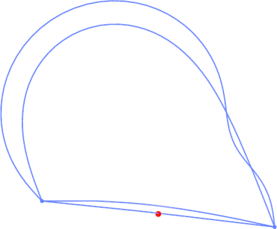
Figure 14: $(\mathcal{A}_{m}^{\partial})^{h}$ Curvature flow towards an infinite geodesic in the elliptic plane. The solutions $\vec{X}^{m}$ at times $t=10^{-3},10^{-2},0.1,1$. On the right we visualize $\vec{\Phi}(\vec{X}^{m})$ at the same times, for (2.73), with the north pole, $\vec{e}_{3}$, represented by a red dot.

4.3 Geodesic evolution equations

In order to demonstrate the possibility to compute geodesic evolution laws with the introduced approximations, we present a computation for geodesic curvature flow on a Clifford torus. To this end, we employ the metric induced by (2.73) with $\mathfrak{s}=1$, so that the torus has radii $r=1$ and $R=2^{\frac{1}{2}}$. As initial data we choose a circle in $H$ with radius $4$ and centre $(0,2)^{T}$. For the simulation in Figure 15 we use the scheme $(\mathcal{A}_{m})^{h}$ with the discretization parameters $J=256$ and $\Delta t=10^{-3}$. In $H$ it can be observed that the initial circle deforms and shrinks to a point. On the surface $\mathcal{M}=\vec{\Phi}(H)$, the initial curve is homotopic to a point, and so unravels and then shrinks to a point.

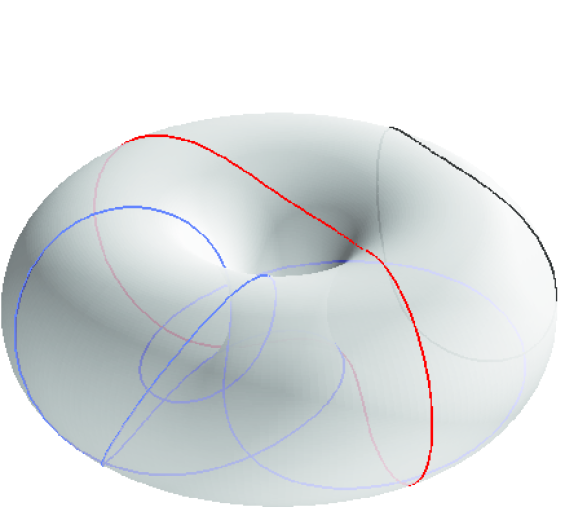
Figure 15: $(\mathcal{A}_{m})^{h}$ Geodesic curvature flow on a Clifford torus. The solutions $\vec{X}^{m}$ at times $t=0,1,10,20,30,39$. On the right we visualize $\vec{\Phi}(\vec{X}^{m})$ at times $t=0,30,39$, for (2.73) with $\mathfrak{s}=1$.

Conclusions

We have derived and analysed various finite element schemes for the numerical approximation of curve evolutions in two-dimensional Riemannian manifolds. The considered evolution laws include curvature flow, curve diffusion and elastic flow. The Riemannian manifolds that can be considered in our framework include the hyperbolic plane, the hyperbolic disk and the elliptic plane. More generally, any metric conformal to the two-dimensional Euclidean metric can be considered. We mention that locally this is always possible for two-dimensional Riemannian manifolds. An example of this are two-dimensional surfaces in ${\mathbb{R}}^{d}$, $d\geq 3$, which are conformally parameterized. Our approach also allows computations for geometric evolution equations of axisymmetric hypersurfaces in ${\mathbb{R}}^{d}$, $d\geq 3$.

For the standard Euclidean plane our proposed schemes collapse to variants introduced by the authors in much earlier papers, see ??.

Appendix A Some exact circular solutions

Here we state some exact solutions for the three geometric evolution equations we consider, i.e. (2.22), (2.36) and (2.55), for selected metrics $g$.

A.1 The hyperbolic plane

Here we consider circular solutions in the hyperbolic plane, based on the exact solution for hyperbolic elastic flow from ?, Lemma 3.1.

In particular, we make the ansatz

$$\vec{x}(\rho,t)=a(t)\,\vec{e}_{2}+r(t)\left[\cos 2\,\pi\,\rho\,\vec{e}_{1}+\sin 2\,\pi\,\rho\,\vec{e}_{2}\right]\qquad\rho\in I\,,$$ (A.1)

for $a(t)>r(t)>0$ for all $t\in[0,T]$. Then it follows from (2.17) for $\mu=1$ that

$$\varkappa_{g}(\rho,t)=\frac{a(t)}{r(t)}\qquad\qquad\rho\in I\,,\ t\in[0,T]\,.$$ (A.2)

Moreover, it holds that

$$\mathcal{V}_{g}=(\vec{x}\,.\,\vec{e}_{2})^{-1}\,\vec{x}_{t}\,.\,\vec{\nu}=-\left(a(t)+r(t)\,\sin 2\,\pi\,\rho\right)^{-1}\,\left[a^{\prime}(t)\,\sin 2\,\pi\,\rho+r^{\prime}(t)\right].$$ (A.3)

We now consider curvature flow, (2.22). With the ansatz (A.1), on noting (A.2) and (A.3), we have that (2.22) reduces to

$$a^{\prime}(t)\,\sin 2\,\pi\,\rho+r^{\prime}(t)=-(a(t)+r(t)\,\sin 2\,\pi\,\rho)\,\frac{a(t)}{r(t)}\,.$$ (A.4)

Differentiating (A.4) with respect to $\rho$ yields that $a^{\prime}(t)=-a(t)$, and hence $a(t)=e^{-t}\,a(0)$. Combining this with (A.4) yields that

$$r^{\prime}(t)=-a(t)\,\frac{a(t)}{r(t)}\qquad\Rightarrow\quad\tfrac{1}{2}\,\frac{\rm d}{{\rm d}t}r^{2}(t)=-a^{2}(t)=-e^{-2\,t}\,a^{2}(0)\,.$$

Hence

$$r^{2}(t)-r^{2}(0)=-2\,a^{2}(0)\,\int_{0}^{t}e^{-2\,u}\;{\rm d}u=-2\,a^{2}(0)\left[-\tfrac{1}{2}\,e^{-2\,t}+\tfrac{1}{2}\right]=a^{2}(0)\left[e^{-2\,t}-1\right],$$

and so (A.1) with

$$a(t)=e^{-t}\,a(0)\,,\quad r(t)=\left(r^{2}(0)-a^{2}(0)\left[1-e^{-2\,t}\right]\right)^{\frac{1}{2}}$$ (A.5)

is a solution to (2.22). We observe that circles move towards the $\vec{e}_{1}$–axis and shrink as they do so. The finite extinction time is $T_{0}=-\frac{1}{2}\,\ln\left[1-\left(\frac{r(0)}{a(0)}\right)^{2}\right]$.

As regards (2.36), it is obvious from (A.2) that any solution of the form (A.1) satisfies $\mathcal{V}_{g}=0$, and so circles are stationary solutions for curve diffusion.

Finally, for the elastic flow (2.55), we recall the exact solution for the hyperbolic elastic flow, (2.57), from ?, Lemma 3.1.

With the ansatz (A.1), on noting (A.2) and (A.3), we have that (2.57) reduces to

$$a^{\prime}(t)\,\sin 2\,\pi\,\rho+r^{\prime}(t)=-(a(t)+r(t)\,\sin 2\,\pi\,\rho)\left(\frac{a(t)}{r(t)}-\frac{a^{3}(t)}{2\,r^{3}(t)}\right).$$ (A.6)

Differentiating (A.6) with respect to $\rho$ yields that

$$a^{\prime}(t)=-r(t)\left(\frac{a(t)}{r(t)}-\frac{a^{3}(t)}{2\,r^{3}(t)}\right),$$ (A.7)

and combining this with (A.6) yields that

$$r^{\prime}(t)=-a(t)\left(\frac{a(t)}{r(t)}-\frac{a^{3}(t)}{2\,r^{3}(t)}\right).$$ (A.8)

On setting

$$\sigma(t)=\frac{a(t)}{r(t)}>1\qquad\Rightarrow\quad\sigma^{\prime}(t)=\frac{a^{\prime}(t)}{r(t)}-\frac{a(t)\,r^{\prime}(t)}{r^{2}(t)}\,,$$ (A.9)

it follows from (A.7) and (A.8) that

$$\sigma^{\prime}(t)=\sigma(t)\,(1-\tfrac{1}{2}\,\sigma^{2}(t))\,(\sigma^{2}(t)-1)\,,$$ (A.10)

which agrees with (3.4) in ? for $\lambda=0$. If $\sigma$ denotes a solution to (A.10), then it follows from (A.7) that $a$ and $r$ satisfy

$$\frac{\rm d}{{\rm d}t}\,\ln a(t) =\frac{a^{\prime}(t)}{a(t)}=\tfrac{1}{2}\,\sigma^{2}(t)-1\quad\Rightarrow\ a(t)=a(0)\,\exp\left(-t+\tfrac{1}{2}\,\int_{0}^{t}\sigma^{2}(u)\;{\rm d}u\right),$$ (A.11a)

$$r(t) =\frac{a(t)}{\sigma(t)}\,.$$ (A.11b)

On recalling that $\sigma(t)>1$, we note that $\sigma(t)=2^{\frac{1}{2}}$ is the only steady state solution of (A.10), and hence circles with ratios $\sigma(t)=2^{\frac{1}{2}}$ are steady state solutions of (2.57). Moreover, circles with $\sigma(t)>2^{\frac{1}{2}}$ will rise and expand indefinitely in time, reducing the ratio $\sigma(t)>2^{\frac{1}{2}}$ as they do so. On the other hand, circles with $\sigma(t)<2^{\frac{1}{2}}$ will sink and shrink indefinitely in time, increasing the ratio $\sigma(t)<2^{\frac{1}{2}}$ as they do so.

In order to compute solutions to (A.10) in practice, we let $F(y)=y^{-1}\,|1-\tfrac{1}{2}\,y^{2}|^{-\frac{1}{2}}\,(y^{2}-1)$, so that $F\in C^{\infty}((1,2^{\frac{1}{2}})\cup(2^{\frac{1}{2}},\infty))$. Then $F^{\prime}(y)=y^{-2}\,(1-\tfrac{1}{2}\,y^{2})^{-1}\,|1-\tfrac{1}{2}\,y^{2}|^{-\frac{1}{2}}$, and hence a solution $\sigma$ to (A.10) satisfies

$$\frac{\rm d}{{\rm d}t}\,F(\sigma(t))=\sigma^{\prime}(t)\,F^{\prime}(\sigma(t))=\frac{\sigma^{2}(t)-1}{\sigma(t)\,|1-\tfrac{1}{2}\,\sigma^{2}(t)|^{\frac{1}{2}}}=F(\sigma(t))\,,$$ (A.12)

which means that a solution $\sigma$ to (A.10) satisfies the nonlinear equation

$$F(\sigma(t))=F(\sigma(0))\,e^{t}\,.$$ (A.13)

A.2 The hyperbolic disk and the elliptic plane

Here we consider the metric (2.6). For $\alpha=1$ we then obtain exact solutions for the hyperbolic disk, while $\alpha=-1$ corresponds to the elliptic plane. In the latter case these solutions can be related to the exact solutions for the corresponding geodesic flows on the sphere from ?, recall §2.4.

In particular, on making the ansatz

$$\vec{x}(\rho,t)=r(t)\left[\cos 2\,\pi\,\rho\,\vec{e}_{1}+\sin 2\,\pi\,\rho\,\vec{e}_{2}\right]\qquad\rho\in I\,,$$ (A.14)

for $r(t)>0$ for all $t\in[0,T]$, it follows from (2.18) that

$$\varkappa_{g}(\rho,t)=\tfrac{1}{2}\left(1+\alpha\,r^{2}(t)\right)[r(t)]^{-1}\qquad\qquad\rho\in I\,,\ t\in[0,T]\,.$$ (A.15)

Moreover, it holds that

$$\mathcal{V}_{g}=g^{\frac{1}{2}}(\vec{x})\,\vec{x}_{t}\,.\,\vec{\nu}=-2\,(1-\alpha\,r^{2}(t))^{-1}\,r^{\prime}(t)\,.$$ (A.16)

We now consider curvature flow, (2.22). It follows from (A.16) and (A.15) that

$$\frac{\rm d}{{\rm d}t}\,r^{2}(t)=\tfrac{1}{2}\left(\alpha^{2}\,r^{4}(t)-1\right)\,.$$ (A.17)

Clearly, if $\alpha=0$ then $r(t)=[r^{2}(0)-\tfrac{1}{2}\,t]^{\frac{1}{2}}$ is the well-known shrinking circle solution for Euclidean curvature flow. For $\alpha\not=0$, in order to compute solutions to (A.17) in practice, we let $G(y)=\left|(1+\alpha\,y^{2})^{-1}\,(1-\alpha\,y^{2})\right|^{\frac{1}{\alpha}}$, so that $G\in C^{\infty}((0,|\alpha|^{-\frac{1}{2}})\cup(|\alpha|^{-\frac{1}{2}},\infty))$, recall also (2.6). Then $G^{\prime}(y)=4\,y\,(\alpha^{2}\,y^{4}-1)^{-1}\,G(y)$ and hence a solution to (A.17) satisfies

$$\frac{\rm d}{{\rm d}t}\,G(r(t))=r^{\prime}(t)\,G^{\prime}(r(t))=G(r(t))\,,$$ (A.18)

which means that a solution to (A.17) satisfies the nonlinear equation

$$G(r(t))=G(r(0))\,e^{t}\,,$$ (A.19)

which can be inverted explicitly. In the case $\alpha=-1$, we recall from (2.73) that the circle (A.14) of radius $r(t)$ in the elliptic plane corresponds to a circle of radius $R(t)=2\,(1+r^{2}(t))^{-1}\,r(t)$, and at height $(r^{2}(t)+1)^{-1}\,(r^{2}(t)-1)$, on the unit sphere in ${\mathbb{R}}^{3}$. It can be easily shown that if $r(t)$ satisfies (A.19) for $\alpha=-1$, then

$$R(t)=[1-(1-R^{2}(0))\,e^{2\,t}]^{\frac{1}{2}}\,,$$ (A.20)

which is the solution of geodesic curvature flow on the unit sphere, given by ?, (5.6). Observe that for $R(0)\in(0,1)$, the finite extinction time is $T_{0}=\tfrac{1}{2}\,\ln\frac{1}{1-R^{2}(0)}$.

As regards (2.36), it is obvious from (A.15) that any solution of the form (A.14) satisfies $\mathcal{V}_{g}=0$, and so circles centred at the origin are stationary solutions to curve diffusion for (2.6).

Finally, we consider the elastic flow (2.55). With the ansatz (A.14), on noting (A.15), (A.16) and (2.9), we have that (2.55) reduces to

$$-2\,(1-\alpha\,r^{2}(t))^{-1}\,r^{\prime}(t)=-\tfrac{1}{16}\,(1+\alpha\,r^{2}(t))^{3}\,r^{-3}(t)+\tfrac{1}{2}\,\alpha\,(1+\alpha\,r^{2}(t))\,r^{-1}(t)\,.$$ (A.21)

This implies the ODE

$$\frac{\rm d}{{\rm d}t}\,r^{4}(t) =\tfrac{1}{8}\,(1-\alpha^{2}\,r^{4}(t))\,(1-6\,\alpha\,r^{2}(t)+\alpha^{2}\,r^{4}(t))\,.$$ (A.22)

In the case $\alpha=-1$, we recall from (2.73) that the circle (A.14) of radius $r(t)$ in the elliptic plane corresponds to a circle of radius $R(t)=2\,(1+r^{2}(t))^{-1}\,r(t)$, and at height $(r^{2}(t)+1)^{-1}\,(r^{2}(t)-1)$, on the unit sphere in ${\mathbb{R}}^{3}$. It can be easily shown that if $r(t)$ satisfies (A.22) for $\alpha=-1$, then $R(t)$ satisfies $\frac{\rm d}{{\rm d}t}\,R^{4}(t)=2\,(1-R^{4}(t))$, i.e.

$$R(t)=[1-(1-R^{4}(0))\,e^{-2\,t}]^{\frac{1}{4}},$$ (A.23)

which is the solution for geodesic elastic flow on the unit sphere given by ?, (5.7). Hence in the case $\alpha=-1$ we can obtain $r(t)$ from

$$r(t)=R^{-1}(t)\,\begin{cases}(1+[1-R^{2}(t)]^{\frac{1}{2}})&r(0)\geq 1\,,\\ (1-[1-R^{2}(t)]^{\frac{1}{2}})&r(0)<1\,,\end{cases}\quad\text{where}\quad R(t)=[1-(1-R^{4}(0))\,e^{-2\,t}]^{\frac{1}{4}}\,,$$ (A.24)

with $R(0)=2\,(1+r^{2}(0))^{-1}\,r(0)$.

Finally, for the case $\alpha=1$, it follows from (A.22) that

$$\frac{\rm d}{{\rm d}t}\,r^{4}(t) =\tfrac{1}{8}\,(1-r^{4}(t))\,(1-6\,r^{2}(t)+r^{4}(t))\,.$$ (A.25)

We note, on recalling (2.6), that $r(t)=2^{\frac{1}{2}}-1$ is a stable stationary solution to (A.25). Hence circles with larger radii will shrink, and circles with smaller radii will expand. In order to solve (A.25) in practice, we define $Q(y)=(1+y^{2})^{-1}\,|1-6\,y^{2}+y^{4}|^{-\frac{1}{2}}\,(1-y^{2})^{2}$, so that $Q\in C^{\infty}((0,2^{\frac{1}{2}}-1)\cup(2^{\frac{1}{2}}-1,1))$ with $Q^{\prime}(y)=32\,(1-y^{4})^{-1}\,(1-6\,y^{2}+y^{4})^{-1}\,y^{3}\,Q(y)$. Hence $\frac{\rm d}{{\rm d}t}\,Q(r(t))=Q(r(t))$, and so a solution to (A.25) satisfies the nonlinear equation

$$Q(r(t))=Q(r(0))\,e^{t}\,.$$ (A.26)

We remark that an alternative to (A.24) for the case $\alpha=-1$ is to solve, similarly to (A.26), the nonlinear equation $Q_{-}(r(t))=Q_{-}(r(0))\,e^{t}$, where $Q_{-}(y)=(1-y^{2})^{-1}\,(1+6\,y^{2}+y^{4})^{-\frac{1}{2}}\,(1+y^{2})^{2}$.

Appendix B Geodesic curve evolution equations

Let $\vec{\Phi}:H\to{\mathbb{R}}^{d}$ be a conformal parameterization of an embedded two-dimensional Riemannian manifold $\mathcal{M}\subset{\mathbb{R}}^{d}$, i.e. $\mathcal{M}=\vec{\Phi}(H)$ and $|\partial_{\vec{e}_{1}}\vec{\Phi}(\vec{z})|^{2}=|\partial_{\vec{e}_{2}}\vec{\Phi}(\vec{z})|^{2}$ and $\partial_{\vec{e}_{1}}\vec{\Phi}(\vec{z})\,.\,\partial_{\vec{e}_{2}}\vec{\Phi}(\vec{z})=0$ for all $\vec{z}\in H$. Given the parameterization $\vec{x}:I\to H$ of the closed curve $\Gamma\subset H$, we let $\vec{y}=\vec{\Phi}\circ\vec{x}$ be a parameterization of $\mathcal{G}\subset\mathcal{M}$. We now show that geodesic curvature flow, geodesic curve diffusion and geodesic elastic flow for $\mathcal{G}=\vec{y}(I)$ on $\mathcal{M}$ reduce to (2.22), (2.36) and (2.55) for the metric $g$ defined by

$$g(\vec{z})=|\partial_{\vec{e}_{1}}\vec{\Phi}(\vec{z})|^{2}=|\partial_{\vec{e}_{2}}\vec{\Phi}(\vec{z})|^{2}\qquad\vec{z}\in H\,.$$ (B.1)

For later use we observe that

$$D\,\vec{\Phi}(\vec{z})\,\vec{v}\,.\,D\,\vec{\Phi}(\vec{z})\,\vec{w}=g(\vec{z})\,\vec{v}\,.\,\vec{w}\qquad\forall\ z\in H\,,\ \vec{v},\vec{w}\in{\mathbb{R}}^{2}\,,$$ (B.2)

where $D\,\vec{\Phi}(\vec{z})=[\partial_{\vec{e}_{1}}\,\vec{\Phi}(\vec{z})\ \partial_{\vec{e}_{2}}\,\vec{\Phi}(\vec{z})]\in{\mathbb{R}}^{d\times 2}$ for $\vec{z}\in H$. A simple computation, on noting (B.2) and (2.1), yields that

$$\vec{y}_{\rho}=D\,\vec{\Phi}(\vec{x})\,\vec{x}_{\rho}\quad\Rightarrow\quad|\vec{y}_{\rho}|=g^{\frac{1}{2}}(\vec{x})\,\vec{x}_{\rho}=|\vec{x}_{\rho}|_{g}\,.$$ (B.3)

Hence it follows from (2.11) that

$$\partial_{s_{y}}=|\vec{y}_{\rho}|^{-1}\,\partial_{\rho}=|\vec{x}_{\rho}|_{g}^{-1}\,\partial_{\rho}=\partial_{s_{g}}\,,$$ (B.4)

and so the unit tangent to the curve $\vec{y}(I)$ is given by

$$\vec{\tau}_{\mathcal{M}}=\vec{y}_{s_{y}}=D\,\vec{\Phi}(\vec{x})\,\vec{x}_{s_{g}}=D\,\vec{\Phi}(\vec{x})\,\vec{\tau}_{g}\,,$$ (B.5)

on recalling (2.12). Similarly, we define the normal $\vec{\nu}_{\mathcal{M}}$ as the unit normal to $\vec{y}(I)$ that is perpendicular to $\vec{\tau}_{\mathcal{M}}$ and that lies in the tangent space to $\mathcal{M}$, i.e.

$$\vec{\nu}_{\mathcal{M}} =(\vec{x}_{s_{g}}\,.\,\vec{e}_{1}\,\partial_{\vec{e}_{2}}\,\vec{\Phi}(\vec{x})-\vec{x}_{s_{g}}\,.\,\vec{e}_{2}\,\partial_{\vec{e}_{1}}\,\vec{\Phi}(\vec{x}))=D\,\vec{\Phi}(\vec{x})\,[-\vec{x}_{s_{g}}^{\perp}]=D\,\vec{\Phi}(\vec{x})\,\vec{\nu}_{g}\,,$$ (B.6)

where we have recalled (2.12). Note that (B.6), in the case $d=3$, agrees with the definition of $\vec{\nu}_{\mathcal{M}}$ in ?, p. 10. We further note from (B.5) that $\vec{y}_{s_{y}s_{y}}$ is perpendicular to $\vec{\tau}_{\mathcal{M}}$, and hence

$$\vec{y}_{s_{y}s_{y}}=\varkappa_{\mathcal{M}}\,\vec{\nu}_{\mathcal{M}}+\vec{\varkappa}_{F}\,,$$ (B.7)

where $\vec{\varkappa}_{F}$ is normal to $\mathcal{M}$, and where $\varkappa_{\mathcal{M}}$ denotes the geodesic curvature of $\vec{y}(I)$.

Clearly, it follows from (B.3) that the length of $\vec{y}(I)$ is given by

$$L_{\mathcal{M}}(\vec{y})=\int_{I}|\vec{y}_{\rho}|\;{\rm d}\rho=\int_{I}|\vec{x}_{\rho}|_{g}\;{\rm d}\rho=L_{g}(\vec{x})\,.$$ (B.8)

We compute, on noting (B.8), (B.4), (B.7), (B.6), (B.2), (2.13) and (2.12), that

$$\frac{\rm d}{{\rm d}t}\,L_{\mathcal{M}}(\vec{y}) =\int_{I}\frac{\vec{y}_{\rho}}{|\vec{y}_{\rho}|}\,.\,(\vec{y}_{\rho})_{t}\;{\rm d}\rho=-\int_{I}\left(\frac{\vec{y}_{\rho}}{|\vec{y}_{\rho}|}\right)_{\rho}\,.\,\vec{y}_{t}\;{\rm d}\rho=-\int_{I}\vec{y}_{s_{y}s_{y}}\,.\,\vec{y}_{t}\,|\vec{y}_{\rho}|\;{\rm d}\rho$$

$$=-\int_{I}\varkappa_{\mathcal{M}}\,\vec{\nu}_{\mathcal{M}}\,.\,\vec{y}_{t}\,|\vec{y}_{\rho}|\;{\rm d}\rho=-\int_{I}\varkappa_{\mathcal{M}}\,D\,\vec{\Phi}(\vec{x})\,\vec{\nu}_{g}\,.\,D\,\vec{\Phi}(\vec{x})\,\vec{x}_{t}\,|\vec{x}_{\rho}|_{g}\;{\rm d}\rho$$

$$=-\int_{I}\varkappa_{\mathcal{M}}\,g(\vec{x})\,\vec{\nu}_{g}\,.\,\vec{x}_{t}\,|\vec{x}_{\rho}|_{g}\;{\rm d}\rho=-\int_{I}\varkappa_{\mathcal{M}}\,\mathcal{V}_{g}\,|\vec{x}_{\rho}|_{g}\;{\rm d}\rho\,.$$ (B.9)

It follows from (B.9), (2.15) and (B.8) that

$$\varkappa_{g}=\varkappa_{\mathcal{M}}\,.$$ (B.10)

In addition we have from (B.6), (B.2), (2.12) and (2.13) that

$$\mathcal{V}_{\mathcal{M}}=\vec{y}_{t}\,.\,\vec{\nu}_{\mathcal{M}}=D\,\vec{\Phi}(\vec{x})\,\vec{x}_{t}\,.\,D\,\vec{\Phi}(\vec{x})\,\vec{\nu}_{g}=\mathcal{V}_{g}\,.$$ (B.11)

Hence the flow (2.22) for $\vec{x}(I)$ in $H$ is equivalent to the flow

$$\mathcal{V}_{\mathcal{M}}=\varkappa_{\mathcal{M}}$$ (B.12)

for $\vec{y}(I)$ on $\mathcal{M}$, which is the so-called geodesic curvature flow, see also ?, (2.19) for the case $d=3$.

Similarly, it follows from (B.11), (B.10) and (B.4) that the flow (2.36) for $\vec{x}(I)$ in $H$ is equivalent to the the geodesic curve diffusion flow

$$\mathcal{V}_{\mathcal{M}}=-(\varkappa_{\mathcal{M}})_{s_{g}s_{g}}\,,$$ (B.13)

see also ?, (2.20) for the case $d=3$. Finally, in order to relate (2.55) for $d=3$ to geodesic elastic flow, i.e. the $L^{2}$–gradient flow of

$$\tfrac{1}{2}\,\int_{I}\varkappa_{\mathcal{M}}^{2}\,|\vec{y}_{\rho}|\;{\rm d}\rho=\tfrac{1}{2}\,\int_{I}\varkappa_{g}^{2}\,|\vec{x}_{\rho}|_{g}\;{\rm d}\rho=W_{g}(\vec{x})\,,$$ (B.14)

recall (B.10), (B.3) and (2.3), we note from from ?, (2.32) that geodesic elastic flow for $\vec{y}(I)$ on $\mathcal{M}$ is given by

$$\mathcal{V}_{\mathcal{M}}=-(\varkappa_{\mathcal{M}})_{s_{y}s_{y}}-\tfrac{1}{2}\,\varkappa_{\mathcal{M}}^{3}-\mathcal{K}(\vec{y})\,\varkappa_{\mathcal{M}}\,,$$ (B.15)

where $\mathcal{K}(\vec{z})$ denotes the Gaussian curvature of $\mathcal{M}$ at $\vec{z}\in\mathcal{M}$. It follows from (B.11), (B.10), (B.4) and (2.72) that (B.15) and (2.55) are equivalent.

Acknowledgements
The authors gratefully acknowledge the support of the Regensburger Universitätsstiftung Hans Vielberth.