Tensor product method for fast solution of optimal control problems with fractional multidimensional Laplacian in constraints

Abstract

We introduce the tensor numerical method for solution of the $d$-dimensional optimal control problems with fractional Laplacian type operators in constraints discretized on large $n^{\otimes d}$ tensor-product Cartesian grids. The approach is based on the rank-structured approximation of the matrix valued functions of the corresponding fractional finite difference Laplacian. We solve the equation for the control function, where the system matrix includes the sum of the fractional $d$-dimensional Laplacian and its inverse. The matrix valued functions of discrete Laplace operator on a tensor grid are diagonalized by using the fast Fourier transform (FFT). Then the low rank approximation of the $d$-dimensional tensors obtained by folding of the corresponding large diagonal matrices of eigenvalues are computed, which allows to solve the governing equation for the control function in a tensor-structured format. The existence of low rank canonical approximation to the class of matrix valued functions involved is justified by using the sinc quadrature approximation method applied to the Laplace transform of the generating function. The linear system of equations for the control function is solved by the PCG iterative method with the rank truncation at each iteration step, where the low Kronecker rank preconditioner is precomputed. The right-hand side, the solution vector, and the governing system matrix are maintained in the rank-structured tensor format which beneficially reduces the numerical cost to $O(n\log n)$, outperforming the standard FFT based methods of complexity $O(n^{3}\log n)$ for 3D case. Numerical tests for the 2D and 3D control problems confirm the linear complexity scaling of the method in the univariate grid size $n$.

1 Introduction

Optimization problems with partial differential equations (PDEs) as constraints are well known in the mathematical literature and have been studied for many years, see [45, 48, 28] for comprehensive presentation. A major challenge in the numerical analysis of the PDE constrained optimal control problems is the evaluation of the constraints requiring the solution of a partial differential or nonlocal integral-differential equations in $\mathbb{R}^{d}$. Therefore, to make these problems tractable, specially tailored solvers are required. In the classical sense, partial differential equations are governed by local operators, implying the sparsity of the discrete operator (matrix). In this case, traditional elliptic problem solvers for the forward problem can be modified to apply to the optimization problems, see [8, 24] for an overview. Multigrid methods for elliptic equations are shown to be efficient since their computational complexity is linear in the number of grid points in the computational domain in $\mathbb{R}^{d}$, see [9, 10].

Recently, study of the problems with nonlocal constraints, where the operator is of integral type, has attracted growing interest. In particular, the problems including the fractional Laplacian operator $(-\Delta)^{\alpha}$, for $0<\alpha\leq 1$, can be applied for modeling of complex systems [1, 5]. Several definitions of fractional elliptic operator based on either integral or spectral formulations have been considered in the literature [44, 20, 25, 40, 41, 46]. The main distinction between the integral and spectral definitions is that the first one admits a nonlocal boundary condition, while the spectral formulation requires only the local boundary condition [41]. A number of application fields motivating the use of fractional power of elliptic operators, for example in biophysics, mechanics, nonlocal electrostatics and image processing have been discussed in [3, 2, 17, 50, 18, 26, 30]. In such applications control problems arise consistently.

In order to illustrate our problem formulation, we notice that in [2] it is shown that heat diffusion in special materials, called ”plasmonic nanostructure networks” [7], which have strong relation to new composite materials, is described exactly by fractional Laplacian operator. This means that the interpretation for the case $\alpha=1$ in the form of distributed control of the heat equation can be carried immediately over to the control of heat equation in the particular material (see also [46]). In our particular application one of the motivations to use the fractional elliptic operators ${\cal L}^{\alpha}$, $\alpha\in(0,1]$, in constraints is due to the opportunity to control the sharpness (contrast) for the resolution of the control and design functions by tuning the fraction power $\alpha$ in a direction to a smaller value.

Numerical solution of problems with nonlocal operators poses an additional computational challenge: since local information is not sufficient for the evaluation of the operator, the discretized operator will be a dense matrix instead of a sparse one–if implemented in a straightforward way. A number of approaches have been proposed and analyzed in the literature to circumvent these difficulties, see papers [27, 25, 50, 18, 26, 6] considering approximation methods for fractional elliptic operators, and [17, 51] related to time dependent problems. An extension method proposed in [11], reduces a fractional Laplacian problem to a classical Laplacian problem in a higher-dimensional space, and allows to make the problem tractable in some cases, see also recent paper [6], which develops the higher-order approximation methods. A proof of concept for an optimal control solver based on the extension approach is considered in [2].

The above methods based on the standard numerical techniques provide at least linear complexity scaling in the discrete problem size, thus exhibiting an exponential increase of storage and computational complexity in the number of dimensions $d$, as $O(n^{d})$, where $n$ is the univariate grid size for discretizations over product $n^{\otimes d}$ grids in $\mathbb{R}^{d}$. Modern tensor numerical methods allow to reduce the computational cost for multivariate problems from $O(n^{d})$ to $O(n)$. They appeared as a bridging of the tensor decompositions from multilinear algebra [14, 12, 21] with basic results in nonlinear approximation theory on the low-rank separable representation of the multivariate functions and operators [19, 20]. The main idea of tensor numerical methods is to reduce the solution procedures for the multivariate nonlocal integral-differential equations to tensor product operations on one-dimensional data. Nowadays, the development and application of low-rank tensor numerical methods is one of the prior directions in scientific computing [38, 39, 16, 13, 35, 31, 42].

In this article, we introduce the tensor numerical approach for the efficient solution of the optimal control problems with fractional $d$-dimensional Laplacian type operators in constraints. We solve the equation for the control function, where the system matrix includes the sum of the fractional $d$-dimensional Laplacian and its inverse. We propose and analyze the approximate low-rank structure representations of functions of the fractional Laplacian $(-\Delta)^{\alpha}$, and its inverse $(-\Delta)^{-\alpha}$, $\alpha>0$, in the bounded domain in $\mathbb{R}^{d}$, $d=2,3$, by using the canonical tensor format. Algorithmically, the functions of discretized Laplace operator are diagonalized by the FFT transform, and then the low rank approximation of the $d$-dimensional tensors obtained by folding of the corresponding large diagonal matrices of eigenvalues are computed. This allows us to solve the governing equation for the control function in a tensor-structured format. Given the low Kronecker rank preconditioner, the PCG iteration with rank truncation by using the representation of the operator system matrix in the canonical tensor format is introduced. In the three-dimensional case, the multigrid Tucker tensor decomposition is applied, while the canonical rank reduction in a course of iteration is performed by using the tensor transforms based on the Reduced Higher Order SVD (RHOSVD) [37, 31].

The theoretical justification for the low-rank canonical and Tucker tensor approximation of functions of the discrete fractional Laplacian in $\mathbb{R}^{d}$, $d=2,3,$ is provided. The existence of the low-rank canonical decompositions is based on the theory of the sinc-approximation methods applied to the Laplace transform representation of the respective operator/matrix values functions. We show that these low-parametric representations transfer to the solution operator for equation describing the control variable, which includes the sum of a fractional Laplacian and its inverse. In this way the spacial dimensions can be approximately separated resulting in a low-rank tensor structure in the solution vector, provided that the design function in the right-hand side is approximated with the low rank.

The tensor approach introduced in this paper is based on the spectral decomposition of the target operators and applies to the problems discretized on large $n\times n\times n$ Cartesian grids in the 3D box-type domains. The low rank tensor structure of all matrix valued functions involved allows to reduce the numerical cost to the linear scale $O(n\log n)$ in the univariate problem size, contrary to the traditional numerical schemes based on FFT diagonalization, which amount to the linear-logarithmic complexity in the volume size, $O(n^{3}\log n)$. Numerical tests for the 2D and 3D control problems confirm the linear complexity scaling of the method in the univariate grid size $n$. Moreover, the efficient representation of matrix valued functions of fractional Laplacian can be used in various applications as the spectrally close preconditioner for the control problems with the more general elliptic operators in the constraint, and for more general geometries.

Notice that the low-rank tensor method for solution of a fractional time dependent optimal control problems, where the operator in constraints is constructed as a sum of the Riemann-Lioville fractional one-dimensional Laplacian operators (integral Caputo type representation discretized by using one-level Toeplitz matrices) has been considered in [17]. See Remarks 4.2 and 4.4 for the discussion on the special case of “directionally fractional” Laplacian in constraints.

The rest of the paper is organized as follows. Section 2 describes the considered problem setting. Section 3 discusses the FEM/FDM discretization schemes for functions of an elliptic operator, formulates the traditional Lagrange multiplies approach and describes the Kronecker product tensor structure in the functions of discrete Laplacain in $d$ dimensions. Section 4 analyzes the tensor approximation of the inverse to fractional Laplace operator and some other matrix valued functions of fractional Laplacian in $\mathbb{R}^{d}$ arising in representation of the unknown control and design functions. In Section 5 we recall the main definition and basic properties of the canonical and Tucker tensor formats to be applied for tensor approximation and rank truncation. Finally, in Section 6, we collect the results of numerical tests for 2D and 3D examples which confirm the efficiency of the tensor approximation for the considered class of optimal control problems.

2 Problem setting

Our goal is the construction of fast solution schemes for solving the control problems with $d$-dimensional fractional elliptic operators in the constraints. For this reason we confine ourself to the case of box-type domains and to the class of generalized Laplacian type elliptic operators with separable coefficients.

Given the design function $y_{\Omega}\in L^{2}(\Omega)$ on $\Omega:=(0,1)^{d}$, $d=1,2,3$, first, we consider the optimization problem for the cost functional

$$\min_{y,u}J(y,u):=\int_{\Omega}(y(x)-y_{\Omega}(x))^{2}\,dx+\frac{\gamma}{2}\int_{\Omega}u^{2}(x)\,dx,\quad\gamma>0,$$ (2.1)

constrained by the elliptic boundary value problem in $\Omega$ for the state variable $y\in H_{0}^{1}(\Omega)$, and control variable $u$,

$${\cal A}y:=-\nabla^{T}\cdot\mathbb{A}(x)\nabla y=\beta u,\quad x\in\Omega,\;u\in L_{2}(\Omega),\quad\beta>0,$$ (2.2)

endorsed with the homogeneous Dirichlet boundary conditions on $\Gamma=\partial\Omega$, i.e., $y_{|\Gamma}=0$. The coefficient matrix $\mathbb{A}(x)\in\mathbb{R}^{d\times d}$ is supposed to be symmetric, positive definite and uniformly bounded in $\Omega$ with positive constants $c>0$ and $C>0$, i.e.,

$$c\,I_{d\times d}\leq\mathbb{A}(x)\leq C\,I_{d\times d}.$$

Under above assumptions the associated bilinear form

$$A(u,v)=\int_{\Omega}\mathbb{A}(x)\nabla u(x)\cdot\nabla v(x)\,dx$$

defined on $V\times V$, $V:=\{v\in H_{0}^{1}(\Omega)\}$ is symmetric, coercive and bounded on $V$ with the same constants $c$ and $C$.

In what follows, we describe the tensor method for fast numerical solution of the optimization problem with the generalized constraints

$${\cal A}^{\alpha}y=\beta u(x),\quad x\in\Omega,$$ (2.3)

such that for $0<\alpha\leq 1$, the fractional power of the elliptic operator ${\cal A}$ is defined by

$${\cal A}^{\alpha}y(x)=\sum_{i=1}^{\infty}\lambda_{i}^{\alpha}c_{i}\psi_{i}(x),\quad y=\sum_{i=1}^{\infty}c_{i}\psi_{i}(x),$$ (2.4)

where $\{\psi_{i}(x)\}_{i=1}^{\infty}$ is the set of $L_{2}$-orthogonal eigenfunctions of the symmetric, positive definite operator ${\cal A}$, while $\{\lambda_{i}\}_{i=1}^{\infty}$ are the corresponding (real and positive) eigenvalues.

In the present paper, we consider the particular case of fractional Laplacian in the form

$${\cal A}^{\alpha}:=(\sum\limits_{\ell=1}^{d}-\Delta_{\ell})^{\alpha},\quad\alpha>0,$$ (2.5)

where $\Delta_{\ell}$ is the 1D Laplacian in variable $x_{\ell}$.

Notice that the elliptic operator inverse ${\cal A}^{-1}={\cal T}:L_{2}(\Omega)\to V$, where ${\cal A}={\cal T}^{-1}$, provides the explicit representation for the state variable, $y=\beta{\cal T}u=\beta{\cal A}^{-1}u$ in case (2.2), while in the general case (2.3) we have

$$y=\beta{\cal T}^{\alpha}u\equiv\beta{\cal A}^{-\alpha}u.$$ (2.6)

Here ${\cal T}$ is a compact, symmetric and positive definite operator on $L_{2}(\Omega)$ and its eigenpairs $\{\psi_{i},\mu_{i}\}$, $i=1,\dots,\infty$, provide an orthonormal basis for $L_{2}(\Omega)$, where we have $\mu_{i}=\lambda_{i}^{-1}$.

There are several representations (definitions) for the fractional power of the symmetric, positive definite operators ${\cal A}^{\alpha}$ and ${\cal A}^{-\alpha}$ with $0<\alpha\leq 1$, see for example the survey papers [40, 41]. In particular, the Dunford-Taylor-Cauchy contour integral, the Laplace transform integral representations and the spectral definitions could be applied.

In the presented computational schemes based on low rank tensor decompositions, we apply the spectral definition and use the Laplace transform integral representation for the analysis and justification of the low rank tensor approximation. For $\alpha>0$, the integral representation based on the Laplace transform

$${\cal A}^{-\alpha}=\frac{1}{\Gamma(\alpha)}\int_{0}^{\infty}t^{\alpha-1}e^{-t{\cal A}}\,dt$$ (2.7)

suggests the numerical schemes for low rank canonical tensor representation of the operator (matrix) ${\cal A}^{-\alpha}$ by using the sinc quadrature approximations for the integral on the real axis [19],

$$\int_{0}^{\infty}t^{\alpha-1}e^{-t{\cal A}}\,dt\approx\sum\limits_{k=-M}^{M}\hat{c}_{k}t_{k}^{\alpha-1}e^{-t_{k}{\cal A}}=\sum\limits_{k=-M}^{M}c_{k}\bigotimes_{\ell=1}^{d}e^{-t_{k}{A_{\ell}}},$$ (2.8)

applied to the operators composed by a sum of commutable terms,

$${\cal A}=\sum_{\ell=1}^{d}A_{\ell},\quad[A_{\ell},A_{k}]=0,\quad\mbox{for all}\quad\ell,k=1,\cdots,d,$$

which ensures that each summand in (2.8) is separable, i.e. $e^{-t_{k}{\cal A}}=\bigotimes_{\ell=1}^{d}e^{-t_{k}{A_{\ell}}}$. For example, in the case of Laplacian we have the $d$-term decomposition $\Delta=\sum_{\ell=1}^{d}\frac{\partial^{2}}{\partial x_{\ell}^{2}}$ with commutable 1D operators. The efficiency of this tensor approach is justified by the established exponentially fast convergence of the sinc quadratures in the number of separable terms $M$ in (2.8), applied on a class of analytic functions. In the present paper, this techniques is used for both the theoretical analysis of the rank decomposition schemes and for the description of their constructive representation, see Section 4.

Further more, for $\alpha>0$ the Dunford-Taylor (or Dunford-Cauchy) contour integral representation reads (see for example [27, 25, 20])

$${\cal A}^{-\alpha}=\frac{1}{2\pi i}\int_{\cal G}z^{-\alpha}({\cal A}-z{\cal I})^{-1}dz,$$ (2.9)

where the contour ${\cal G}$ in the complex plane includes the spectrum of operator (matrix) ${\cal A}$. This representation applies to any $u\in L_{2}(\Omega)$ and it allows to define the negative fractional powers of elliptic operator as a finite sum of elliptic resolvents ${\cal R}_{z}({\cal L})=(z{\cal I}-{\cal L})^{-1}$ by application of certain quadrature approximations,

$$\int_{\cal G}z^{-\alpha}({\cal A}-z{\cal I})^{-1}dz\approx\sum\limits_{k=1}^{M}c_{k}z_{k}^{-\alpha}({\cal A}-z_{k}{\cal I})^{-1},\quad z_{k}\in{\cal G},$$

similar to (2.8), see also [25, 19, 20]. This opens the way for multigrid based, ${\cal H}$-matrix (see [20]) or tensor-structured schemes approximating the fractional power of elliptic operator with variable coefficients of rather general form and defined on non-rectangular geometries combined with the nested iterations.

It is worth to notice that both integral representations (2.7) and (2.9) can be applied to rather general class of analytic functions of operator $f({\cal A})$, including the case $f({\cal A})=\mathcal{A}^{-\alpha}$, see [27, 19, 20].

The constraints equation (2.6) allows to derive the Lagrange equation for the control $u$ in the explicit form as follows (see §3 concerning the Lagrange equations)

$$\big{(}\beta\mathcal{A}^{-\alpha}+\tfrac{\gamma}{\beta}\mathcal{A}^{\alpha}\big{)}u=y_{\varOmega},$$ (2.10)

for some positive constants $\beta>0$ and $\gamma>0$. This equation implies the following representation for the state variable

$$y=\beta\mathcal{A}^{-\alpha}u.$$ (2.11)

The practically interesting range of parameters includes the case $\beta=O(1)$ for the small values of $\gamma>0$. Our tensor numerical method is designed for solving equations (2.10) and (2.11) that include the nonlocal operators of “integral-differential” type. The efficiency of the rank-structured tensor approximations presupposes that the design function in the right-hand side of these equations, $y_{\varOmega}(x_{1},x_{2},x_{3})$, allows the low rank separable approximation.

Since we aim for the low-rank (approximate) tensor representation of all functions and operators involved in the above control problem, it is natural to assume that the equation coefficients matrix takes a diagonal form

$$\mathbb{A}(x)=\mbox{diag}\{a_{1}(x_{1}),a_{2}(x_{2})\},\quad a_{\ell}(x_{\ell})>0,\quad\ell=1,2,$$

in 2D case, and similar for $d=3$

$$\mathbb{A}(x)=\mbox{diag}\{a_{1}(x_{1}),a_{2}(x_{2}),a_{3}(x_{3})\},\quad a_{\ell}(x_{\ell})>0,\quad\ell=1,2,3,$$ (2.12)

where the $d$-dimensional Laplacian is the particular case with $a_{\ell}(x_{\ell})=const$.

In what follows, we consider the discrete matrix formulation of the optimal control problem (2.1), (2.3) based on the FEM/FDM discretization ${A}_{h}$ of $d$-dimensional Laplacian defined on the uniform $n_{1}\times n_{2}\times\ldots\times n_{d}$ tensor grid in $\Omega$, where $h=h_{\ell}=1/n_{\ell}$ is the univariate mesh parameter. The $L_{2}$ scalar product is substituted by the Euclidean scalar product $(\cdot,\cdot)$ of vectors in $\mathbb{R}^{\bf n}$, ${\bf n}=(n_{1},n_{2},\ldots,n_{d})$.

In this paper, the fractional Laplacian ${\cal A}^{\alpha}$ is approximated by its FEM/FDM representation $({\cal A}_{h})^{\alpha}$, where the matrix $({\cal A}_{h})^{\alpha}$ is defined by spectral decomposition of ${A}_{h}$ in (2.4). The FEM approximation theory for fractional powers of elliptic operator was presented in [1, 18, 26, 30], see also literature therein.

3 Optimality conditions and representations in a low-rank format

The solution of problem (2.1) with constraint (2.3) requires solving for the necessary optimality conditions. In this section, we will derive these conditions based on a discretize-then-optimize-approach. Then, we will discuss how the involved discretized operators can be applied efficiently in a low-rank format, and how this can be used to design a preconditioned conjugate gradient (PCG) scheme for the necessary optimality conditions.

3.1 Discrete optimality conditions

We consider the discretized version of the control problem (2.1)-(2.3). We assume we have a uniform grid in each space dimension, i. e. we have $N=n_{1}n_{2}$ (for $d=2$) or $N=n_{1}n_{2}n_{3}$ (for $d=3$) grid points. We will denote the discretized state $y$, design $y_{\Omega}$ and control $u$ by vectors $\mathbf{y},\mathbf{y}_{\Omega},\mathbf{u}\in{\mathbb{R}}^{N}$, respectively. For simplicity, we assume that we use the same approximation for all quantities.

Then, the discrete problem is given as

$$\min_{\mathbf{y},\mathbf{u}}= \frac{1}{2}(\mathbf{y}-\mathbf{y}_{\Omega})^{T}M(\mathbf{y}-\mathbf{y}_{\Omega})+\frac{\gamma}{2}\mathbf{u}^{T}M\mathbf{u}$$

$$\text{s.\,t.}~{}A^{\alpha}\mathbf{y}= \beta M\mathbf{u},$$

where $A=\mathcal{A}_{h}$ denotes a discretization of the elliptic operator $\mathcal{A}$ by finite elements or finite differences. The matrix $M$ will be a mass matrix in the finite element case and simply the identity matrix in the finite difference case.

For the discrete adjoint $\mathbf{p}$ define the Lagrangian function

$$L(\mathbf{y},\mathbf{u},\mathbf{p})=\frac{1}{2}(\mathbf{y}-\mathbf{y}_{\Omega})^{T}M(\mathbf{y}-\mathbf{y}_{\Omega})+\frac{\gamma}{2}\mathbf{u}^{T}M\mathbf{u}+\mathbf{p}^{T}(A^{\alpha}\mathbf{y}-\beta M\mathbf{u}),$$ (3.1)

and compute the necessary first order conditions, given by the Karush-Kuhn-Tucker (KKT) system,

$$\begin{bmatrix}M&O&A^{\alpha}\\ O&\gamma M&-\beta M\\ A^{\alpha}&-\beta M&O\end{bmatrix}\begin{pmatrix}\mathbf{y}\\ \mathbf{u}\\ \mathbf{p}\\ \end{pmatrix}=\begin{pmatrix}\mathbf{y}_{\varOmega}\\ \mathbf{0}\\ \mathbf{0}\\ \end{pmatrix}.$$ (3.2)

We can solve the state equation for $\mathbf{y}$, getting

$$\mathbf{y}=\beta A^{-\alpha}\mathbf{u},$$

and the design equation for $\mathbf{p}$ getting

$$\mathbf{p}=\tfrac{\gamma}{\beta}\mathbf{u}.$$

Hence the adjoint equation gives us an equation for the control $\mathbf{u}$, namely

$$A_{2}\mathbf{u}\equiv\big{(}\beta A^{-\alpha}+\tfrac{\gamma}{\beta}A^{\alpha}\big{)}\mathbf{u}=\mathbf{y}_{\varOmega}.$$ (3.3)

In this paper, we use the explicit relation (3.3) as the governing equation for calculation of the unknown control $\mathbf{u}$. The main motivation is that the system matrix in equation (3.3), that includes fractional power of the stiffness matrix $A$ and its inverse $A^{-1}$, can be well approximated by the low Kronecker rank matrices. Hence, the reformulation of the traditional system (3.2) in the form (3.3) proves to be convenient for the construction of low-rank tensor approximation to the arising hybrid system matrix $A_{2}$ and for the construction of spectrally close preconditioner by approximation of $A_{2}^{-1}$. Furthermore, notice that the proposed rank-structured approximations for the case of Laplacain type operators can be also gainfully used for preconditioning in the case of more general elliptic operators with variable coefficients in constraints. In what follows, we construct and analyze the low Kronecker rank decompositions of the arising matrix valued functions, see §4.1 and §4.2 below.

3.2 Matrix-vector multiplication in the low-rank format

First, we discuss a Kronecker form decomposition of functions of discrete Laplacian $A=A_{h}$ diagonalized in the Fourier basis, which is compatible with low-rank data. Let $I_{\ell}$ denote the identity matrix, and $A_{(\ell)}$ the discretized one-dimensional Laplacian on the given grid in the $\ell$-th mode, then we have

$$A=A_{(1)}\otimes I_{2}\otimes I_{3}+I_{1}\otimes A_{(2)}\otimes I_{3}+I_{1}\otimes I_{2}\otimes A_{(3)},$$ (3.4)

where $\otimes$ denotes the Kronecker product of matrices. To calculate the matrices $A_{(\ell)}$, we simply discretize the one-dimensional subproblems

$$- y^{\prime\prime}(x_{\ell})=\beta u(x_{\ell})$$

$$y(0)=0=y(1).$$

Using a uniform grid with grid size $h_{\ell}$, we obtain the discretizations

$$\underbrace{-\frac{1}{h_{\ell}}\begin{bmatrix}2&-1&&\\ -1&\ddots&\ddots&\\ &\ddots&\ddots&-1\\ &&-1&2\end{bmatrix}}_{=A_{(\ell)}}\begin{pmatrix}y^{(\ell)}_{1}\\ \vdots\\ y^{(\ell)}_{n_{\ell}}\end{pmatrix}=\beta\begin{pmatrix}u^{(\ell)}_{1}\\ \vdots\\ u^{(\ell)}_{n_{\ell}}\end{pmatrix}$$

The “one-dimensional” matrix $A_{(\ell)}$ has an eigenvalue decomposition in the Fourier basis, i.e.

$$A_{(\ell)}=F_{\ell}^{*}{\varLambda}_{(\ell)}F_{\ell}.$$

In the case of homogeneous Dirichlet boundary conditions the matrix $F_{\ell}$ defines the $\sin$-Fourier transform while ${\varLambda}_{(\ell)}=\mbox{diag}\{\lambda^{(\ell)}_{1},\dots,\lambda^{(\ell)}_{n}\}$, where $\lambda_{k}$ denote the eigenvalues of the univariate discrete Laplacian with Dirichlet boundary conditions. These are given by

$$\lambda_{k}=-\frac{4}{h_{\ell}^{2}}\sin^{2}\bigg{(}\frac{\pi k}{2(n_{\ell}+1)}\bigg{)}=-\frac{4}{h_{\ell}^{2}}\sin^{2}\bigg{(}\frac{\pi kh_{\ell}}{2}\bigg{)}.$$ (3.5)

Thus, using the properties of the Kronecker product, we can write the first summand in (3.4) as

$$\begin{split}A_{1}\otimes I_{2}\otimes I_{3}&=(F_{1}^{*}{\varLambda}_{(1)}F_{1})\otimes(F_{2}^{*}I_{2}F_{2})\otimes(F_{3}^{*}I_{3}F_{3})\\ &=(F_{1}^{*}\otimes F_{2}^{*}\otimes F_{3}^{*})({\varLambda}_{(1)}\otimes I_{2}\otimes I_{3})(F_{1}\otimes F_{2}\otimes F_{3}).\end{split}$$

The decomposition of the second and third summand works analogously, thus we can write equation (3.4) as

$$\begin{split}A=&(F_{1}^{*}\otimes F_{2}^{*}\otimes F_{3}^{*})(\varLambda_{1}\otimes I_{2}\otimes I_{3})(F_{1}\otimes F_{2}\otimes F_{3})\\ &+(F_{1}^{*}\otimes F_{2}^{*}\otimes F_{3}^{*})(I_{1}\otimes\varLambda_{2}\otimes I_{3})(F_{1}\otimes F_{2}\otimes F_{3})\\ &+(F_{1}^{*}\otimes F_{2}^{*}\otimes F_{3}^{*})(I_{1}\otimes I_{2}\otimes\varLambda_{3})(F_{1}\otimes F_{2}\otimes F_{3})\\ =\;&(F_{1}^{*}\otimes F_{2}^{*}\otimes F_{3}^{*})\underbrace{\big{(}\varLambda_{1}\otimes I_{2}\otimes I_{3}+I_{1}\otimes\varLambda_{2}\otimes I_{3}+I_{1}\otimes I_{2}\otimes\varLambda_{3}\big{)}}_{\eqqcolon\varLambda}(F_{1}\otimes F_{2}\otimes F_{3}),\end{split}$$ (3.6)

where $\varLambda\in\mathbb{R}^{n^{3}\times n^{3}}$ is the diagonal matrix. The above expression gives us the eigenvalue factorization (diagonalization) of an analytic matrix valued functions ${\cal F}(A)$ of the matrix $A$,

$$\mathcal{F}(A)=(F_{1}^{*}\otimes F_{2}^{*}\otimes F_{3}^{*})\mathcal{F}(\varLambda)(F_{1}\otimes F_{2}\otimes F_{3}),$$ (3.7)

which can be multiplied with a vector of general structure in $O(n^{3}\log n)$ operations.

In the tensor based scheme, we construct the low Kronecker rank tensor decomposition of the diagonal matrix $\mathcal{F}(\varLambda)\in\mathbb{R}^{n^{3}\times n^{3}}$,

$$\mathcal{F}(\varLambda)=\sum_{k=1}^{R}\operatorname{diag}\big{(}\mathbf{u}_{1}^{(k)}\otimes\mathbf{u}_{2}^{(k)}\otimes\mathbf{u}_{3}^{(k)}\big{)},$$

with vectors $\mathbf{u}_{\ell}^{(k)}\in{\mathbb{R}}^{n_{\ell}}$ and $R\ll\min(n_{1},n_{2},n_{3})$, via canonical approximation of the $n\times n\times n$ tensor obtained by folding of the long vector $\mbox{diag}(\mathcal{F}(\varLambda))\in\mathbb{R}^{n^{3}}$. Then, the low Kronecker rank approximation for $\mathcal{F}(A)$ is obtained by multiplication from left and right with the factorized FFT matrices, see Section 4.

First, we consider the fast calculation of the matrix vector product with $A$. In the case $d=2$, the factorization (3.6) simplifies to

$$\begin{split}A&=(F_{1}^{*}\otimes F_{2}^{*})\underbrace{\big{(}\varLambda_{1}\otimes I_{2}+I_{1}\otimes\varLambda_{2}\big{)}}_{\eqqcolon\varLambda}(F_{1}\otimes F_{2}),\end{split}$$ (3.8)

such that for an analytic function $\mathcal{F}$ applied to $A$, we obtain

$$\mathcal{F}(A)=(F_{1}^{*}\otimes F_{2}^{*})\mathcal{F}(\varLambda)(F_{1}\otimes F_{2}).$$ (3.9)

Now assume that the diagonal matrix $\mathcal{F}(\varLambda)$ can be expressed approximately as a short sum of Kronecker rank-$1$ diagonal matrices, i.e.,

$$\mathcal{F}(\varLambda)=\sum_{k=1}^{R}\operatorname{diag}\big{(}\mathbf{u}_{1}^{(k)}\otimes\mathbf{u}_{2}^{(k)}\big{)},$$

with vectors $\mathbf{u}_{\ell}^{(k)}\in{\mathbb{R}}^{n_{\ell}}$ and $R\ll\min(n_{1},n_{2})$, and, moreover, let $\mathbf{x}\in{\mathbb{R}}^{N}$ be a vector given in a low rank Kronecker form, i. e.

$$\mathbf{x}=\sum_{j=1}^{S}\mathbf{x}_{1}^{(j)}\otimes\mathbf{x}_{2}^{(j)},$$

with vectors $\mathbf{x}_{\ell}^{(j)}\in{\mathbb{R}}^{n_{\ell}}$ and $S\ll\min(n_{1},n_{2})$. Then, we can compute a matrix-vector product

$$\begin{split}\mathcal{F}(A)\mathbf{x}&=(F_{1}^{*}\otimes F_{2}^{*})\bigg{(}\sum_{k=1}^{R}\operatorname{diag}\big{(}\mathbf{u}_{1}^{(k)}\otimes\mathbf{u}_{2}^{(k)}\big{)}\bigg{)}(F_{1}\otimes F_{2})\bigg{(}\sum_{j=1}^{S}\mathbf{x}_{1}^{(j)}\otimes\mathbf{x}_{2}^{(j)}\bigg{)}\\ &=\sum_{k=1}^{R}\sum_{j=1}^{S}F_{1}^{*}\big{(}\mathbf{u}_{1}^{(k)}\odot F_{1}\mathbf{x}_{1}^{(j)}\big{)}\otimes F_{2}^{*}\big{(}\mathbf{u}_{2}^{(k)}\odot F_{2}\mathbf{x}_{2}^{(j)}\big{)},\end{split}$$ (3.10)

where $\odot$ denotes the Hadamard (componentwise) product. Using the sin-FFT, expression (3.10) can be calculated in factored form in $\mathcal{O}(RSn\log n)$ flops, where $n=\max(n_{1},n_{2})$.

Likewise, in the case $d=3$, by completely analogous reasoning, equation (3.10) becomes

$$\mathcal{F}(A)\mathbf{x}=\sum_{k=1}^{R}\sum_{j=1}^{S}F_{1}^{*}\big{(}\mathbf{u}_{1}^{(k)}\odot F_{1}\mathbf{x}_{1}^{(j)}\big{)}\otimes F_{2}^{*}\big{(}\mathbf{u}_{2}^{(k)}\odot F_{2}\mathbf{x}_{2}^{(j)}\big{)}\otimes F_{3}^{*}\big{(}\mathbf{u}_{3}^{(k)}\odot F_{3}\mathbf{x}_{3}^{(j)}\big{)},$$ (3.11)

and similar in the case of $d>3$, which ensure the evaluation cost $\mathcal{O}(dRSn\log n)$.

In our application the matrix function $F(A)$ has the form $F(A)=\big{(}\beta A^{-\alpha}+\tfrac{\gamma}{\beta}A^{\alpha}\big{)}$ and its inverse, $(F(A))^{-1}$. In what follows, we discuss the tensor method for solving the linear system of equations (3.3) in the low-rank formats. To that end, we use the PCG scheme on the “low-rank” manifold sketched in the next paragraph. This algorithm allows the low cost calculations with rank truncations applied to both 2D and 3D cases. In the 3D case, we use the rank truncation in the canonical format by application of the RHOSVD decomposition (see Section 5).

3.3 The low-rank PCG scheme

For operators $\mathtt{func}$ and $\mathtt{precond}$ given in a low-rank format, such as (3.10) (for $d=2$) or (3.11) (for $d=3$), Krylov subspace methods can be applied very efficiently, since they only require matrix-vector products. The formulation of the PCG method in Algorithm 1 is independent of $d$, as long as an appropriate rank truncation procedure $\mathtt{trunc}$ is chosen.

Algorithm 1 Preconditioned CG method in low-rank format

1:Rank truncation procedure $\mathtt{trunc}$, rank tolerance parameter $\varepsilon$, linear function in low rank format $\mathtt{fun}$, preconditioner in low rank format $\mathtt{precond}$, right-hand side tensor $\mathbf{B}$, initial guess $\mathbf{X}^{(0)}$, maximal iteration number $k_{\max}$

2:$\mathbf{R}^{(0)}\leftarrow\mathbf{B}-\mathtt{fun}(\mathbf{X}^{(0)})$

3:$\mathbf{Z}^{(0)}\leftarrow\mathtt{precond}(\mathbf{R}^{(0)})$

4:$\mathbf{Z}^{(0)}\leftarrow\mathtt{trunc}(\mathbf{Z}^{(0)},\varepsilon)$

5:$\mathbf{P}^{(0)}\leftarrow(\mathbf{Z}^{(0)})$

6:$k\leftarrow 0$

7:repeat

8:     $\mathbf{S}^{(k)}\leftarrow\mathtt{fun}(\mathbf{P}^{(k)})$

9:     $\mathbf{S}^{(k)}\leftarrow\mathtt{trunc}(\mathbf{S}^{(k)},\varepsilon)$

10:     $\alpha_{k}\leftarrow\frac{\langle\mathbf{R}^{(k)},\mathbf{Z}^{(k)}\rangle}{\langle\mathbf{P}^{(k)},\mathbf{S}^{(k)}\rangle}$

11:     $\mathbf{X}^{(k+1)}\leftarrow\mathbf{X}^{(k)}+\alpha_{k}\mathbf{P}^{(k)}$

12:     $\mathbf{X}^{(k+1)}\leftarrow\mathtt{trunc}(\mathbf{X}^{(k+1)},\varepsilon)$

13:     $\mathbf{R}^{(k+1)}\leftarrow\mathbf{R}^{(k)}-\alpha_{k}\mathbf{S}^{(k)}$

14:     $\mathbf{R}^{(k+1)}\leftarrow\mathtt{trunc}(\mathbf{R}^{(k+1)},\varepsilon)$

15:     if $\mathbf{R}^{(k+1)}$ is sufficiently small then

16:         return $\mathbf{X}^{(k+1)}$

17:         break

18:     end if

19:     $\mathbf{Z}^{(k+1)}\leftarrow\mathtt{precond}(\mathbf{R}^{(k+1)})$

20:     $\mathbf{Z}^{(k+1)}\leftarrow\mathtt{trunc}(\mathbf{Z}^{(k+1)},\varepsilon)$

21:     $\beta_{k}\leftarrow\frac{\langle\mathbf{R}^{(k+1)},\mathbf{Z}^{(k+1)}\rangle}{\langle\mathbf{Z}^{(k)},\mathbf{R}^{(k)}\rangle}$

22:     $\mathbf{P}^{(k+1)}\leftarrow\mathbf{Z}^{(k+1)}+\beta_{k}\mathbf{P}^{(k)}$

23:      $\mathbf{P}^{(k+1)}\leftarrow\mathtt{trunc}(\mathbf{P}^{(k+1)},\varepsilon)$

24:     $k\leftarrow k+1$

25:until $k=k_{\max}$

26:Solution $\mathbf{X}$ of $\mathtt{fun}(\mathbf{X})=\mathbf{B}$

As the rank truncation procedure, in our implementation we apply the reduced SVD algorithm in 2D case and the RHOSVD based canonical-to-Tucker-to-canonical algorithm (see [37]) as described in Section 5.

4 Low-rank tensor approximation for analytic functions of fractional $d$-dimensional Laplacian

4.1 Rank-structured decomposition for functions of the core diagonal matrix $\Lambda$

In this section we analyze the rank-structured tensor decompositions of various matrix (tensor) valued functions on the discrete Laplacian arising in the solution of problems (2.10) and (2.11) including different combinations of fractional Laplacian in $\mathbb{R}^{d}$. These decompositions provide the short term Kronecker product representations for functions of multidimensional Laplacian.

We consider the matrices $A_{1},A_{2}$ and $A_{3}$ defined as the matrix valued functions of the discrete Laplacian ${A}_{h}$ by the equations

$${A}_{1}={A}_{h}^{-\alpha},$$ (4.1)

$${A}_{2}={A}_{h}^{-\alpha}+{A}_{h}^{\alpha},$$ (4.2)

and

$${A}_{3}=\big{(}{A}_{h}^{-\alpha}+{A}_{h}^{\alpha}\big{)}^{-1}=A_{2}^{-1},$$ (4.3)

respectively. It is worth to notice that the matrix $A_{3}$ defines the solution operator in equation (2.10), which allows to calculate the optimal control in terms of the design function ${\bf y}_{\Omega}$ on the right-hand side of (2.10) by solving the equation

$${A}_{2}{\bf u}^{\ast}={\bf y}_{\Omega}.$$ (4.4)

Finally, the state variable is calculated by

$${\bf y}=\beta{A}_{h}^{-\alpha}{\bf u}^{\ast}=\beta A_{1}{\bf u}^{\ast}.$$ (4.5)

In the presented numerics we consider the rank bounds of the Tucker/canonical (or SVD in the 2D case) decompositions for the corresponding multi-indexed core tensors/matrices $\mathcal{F}(\varLambda_{p})$, $p=1,2,3$, further denoted by $G_{1},G_{2},G_{3}\in\mathbb{R}^{n\times n}$ in the 2D case, and by ${\bf G}_{1},{\bf G}_{2},{\bf G}_{3}\in\mathbb{R}^{n\times n\times n}$ in the 3D case and representing the matrix valued functions $A_{1},A_{2},A_{3}$ of ${A}_{h}$ in the Fourier basis, see (3.7) and (3.9). This factorization is well suited for the rank-structured algebraic operations since the $d$-dimensional Fourier transform matrix has the Kronecker rank equals to one. For example, for $d=3$ we have

$${\cal F}=F_{1}\otimes F_{2}\otimes F_{3}.$$

Let $\{\lambda_{i}\}_{i=1}^{n}$ be the set of eigenvalues for the 1D finite difference Laplacian in $H^{1}_{0}(0,1)$ discretized on the uniform grid with the mesh size $h=1/(n+1)$, see (3.5). The elements of the core diagonal matrix $\varLambda$ in (3.6) can be reshaped to a three-tensor

$${\bf G}=[g(i_{1},i_{2},i_{3})]\in\mathbb{R}^{n_{1}\times n_{2}\times n_{3}},\quad i_{\ell}\in\{1,\ldots,n_{\ell}\},$$

where

$$g(i_{1},i_{2},i_{3})=\lambda_{i_{1}}+\lambda_{i_{2}}+\lambda_{i_{3}},$$

implying that the three-tensor ${\bf G}$ has the exact rank-$3$ canonical decomposition. In the case $d=2$, we have similar two-term representation for the matrices $G=[g(i_{1},i_{2})]\in\mathbb{R}^{n_{1}\times n_{2}}$, $g(i_{1},i_{2})=\lambda_{i_{1}}+\lambda_{i_{2}}$.

In the 3D case we consider the Tucker and canonical decompositions of the $n\times n\times n$ core tensors, corresponding to the matrices $A_{1},A_{2},A_{3}$,

$${\bf G}_{p}=[g_{p}(i,j,k)],\quad p=1,2,3$$ (4.6)

with entries defined by

$$g_{1}(i,j,k)=\frac{1}{(\lambda_{i}+\lambda_{j}+\lambda_{k})^{\alpha}},$$ (4.7)

$$g_{2}(i,j,k)=\frac{1}{(\lambda_{i}+\lambda_{j}+\lambda_{k})^{\alpha}}+(\lambda_{i}+\lambda_{j}+\lambda_{k})^{\alpha},$$ (4.8)

$$g_{3}(i,j,k)=\left((\lambda_{i}+\lambda_{j}+\lambda_{k})^{-\alpha}+(\lambda_{i}+\lambda_{j}+\lambda_{k})^{\alpha}\right)^{-1}.$$ (4.9)

In the 2D case we analyze the singular value decomposition of the $n\times n$ core matrices

$$G_{p}=[g_{p}(i,j)],\quad p=1,\,2,\,3,$$ (4.10)

with entries defined by

$$g_{1}(i,j)=\frac{1}{(\lambda_{i}+\lambda_{j})^{\alpha}},$$ (4.11)

$$g_{2}(i,j)=\frac{1}{(\lambda_{i}+\lambda_{j})^{\alpha}}+(\lambda_{i}+\lambda_{j})^{\alpha},$$ (4.12)

$$g_{3}(i,j)=\left((\lambda_{i}+\lambda_{j})^{-\alpha}+(\lambda_{i}+\lambda_{j})^{\alpha}\right)^{-1}.$$ (4.13)

The error estimate for the rank decomposition of the matrices $G_{p}$ and the respective 3D tensors ${\bf G}_{p}$ can be derived based on the sinc-approximation theory as discussed in §4.2. We consider the class of matrix valued functions of the discrete Laplacian, $A_{1},\ldots,A_{3}$, given by (4.1) – (4.3). In view of the FFT diagonalization, the tensor approximation problem is reduced to the analysis of the corresponding function related tensors ${\bf G}_{1},\ldots,{\bf G}_{3}$ specified by multivariate functions of the discrete argument, $g_{1},\ldots,g_{3}$, given by (4.7) – (4.9).

It is worse to note that the sinc quadrature approximation theory based on the Laplace transform applies only to the operators (matrices) with the negative fractional power like ${{A}_{h}}^{-\alpha}$, $\alpha>0$. To prove the existence of rank decomposition for the positive power of ${A}_{h}$, we notice that for $1>\alpha>0$

$$A^{\alpha}=A\cdot A^{\alpha-1},\quad\alpha-1<0,$$

where the second factor on the right-hand side can be approximated with the low Kronecker rank due to the general theory of sinc approximation, while the initial stiffness matrix $A$ has the Kronecker rank equals to $d$. Similar argument applies to the case $\alpha>1$. This proves the following Lemma.

Lemma 4.1

For given $\alpha>0$, let the matrix $A^{-\beta}$, $\beta>0$, can be represented in the Kronecker rank-$R$ form. Then the matrix $A^{\alpha}$ can be represented with the Kronecker rank at most $d\,R$.

Remark 4.2

Our numerical scheme can be also applied to the class of “directionally fractional” Laplacian-type operators ${\cal A}_{(\alpha)}$, obtained by the essential simplification of the fractional elliptic operator ${\cal A}^{\alpha}$ in (2.5) considered in our paper, as follows

$${\cal A}_{(\alpha)}:=\sum\limits_{\ell=1}^{d}\left(-\Delta_{\ell}\right)^{\alpha},\quad\alpha>0,$$ (4.14)

where $\Delta_{\ell}$ is the 1D Laplacian in variable $x_{\ell}$. In the case $d=3$ the core tensors $g_{p}$ in (4.7) – (4.9) representing the operator ${\cal A}_{(\alpha)}$ in the Fourier basis are simplified to

$$\widetilde{g}_{1}(i,j,k)=\frac{1}{\lambda_{i}^{\alpha}+\lambda_{j}^{\alpha}+\lambda_{k}^{\alpha}},$$ (4.15)

$$\widetilde{g}_{2}(i,j,k)=\frac{1}{\lambda_{i}^{\alpha}+\lambda_{j}^{\alpha}+\lambda_{k}^{\alpha}}+\lambda_{i}^{\alpha}+\lambda_{j}^{\alpha}+\lambda_{k}^{\alpha},$$ (4.16)

$$\widetilde{g}_{3}(i,j,k)=\left(\frac{1}{\lambda_{i}^{\alpha}+\lambda_{j}^{\alpha}+\lambda_{k}^{\alpha}}+\lambda_{i}^{\alpha}+\lambda_{j}^{\alpha}+\lambda_{k}^{\alpha}\right)^{-1},$$ (4.17)

respectively. The low rank tensor decomposition of these discrete functions is practically identical to the case of Laplacian operator in (4.7) – (4.9) corresponding to the fractional power $\alpha=1$. The similar model has been considered in [17] for $d=2,3$, where instead of $(-\Delta_{\ell})^{\alpha}$ the so-called Caputo type integral representation has been adapted. Instead of the Fourier based diagonalization, the QTT tensor approximation [34, 43] of the arising $n\times n$ univariate Toeplitz matrices has been applied.

The application of the tensor techniques to the case of variable coefficients in (4.14) in 3D case requires the solution of the few 1D spectral problems for symmetric three-diagonal $n\times n$ matrices, which on the order of magnitude faster compared with the optimal cost $O(n^{4})$ for solving the 3D control problem in the full matrix format.

Remark 4.3

In the general case of “directionally fractional” operators with variable coefficients $a_{\ell}(x_{\ell})>0$ in (4.14) the orthogonal matrices $F_{\ell}$, $\ell=1,\ldots,d$, of the univariate Fourier transforms in (3.6) should be substituted by the orthogonal matrices of the eigenvalue decomposition for the discretized elliptic operators $A_{h,\ell}$ (1D stiffness matrices) corresponding to the substitution $-\Delta_{\ell}\mapsto A_{\ell}=-\nabla_{\ell}^{T}\cdot a_{\ell}(x_{\ell})\nabla_{\ell}$. The eigenvalues in (4.15) – (4.17) are obtained from the solution of the discrete eigenvalue problem $A_{h,\ell}{\bf u}_{i}=\lambda_{i,\ell}{\bf u}_{i}$, $\ell=1,\ldots,d$.

4.2 Rank estimates for matrix valued functions

In this section, we sketch the proof of the existence of the low rank canonical/Tucker decomposition of the core tensors ${\bf G}_{p}$, $p=1,\ldots,4$. Following [47], we define the Hardy space $H^{1}(D_{\delta})$ of functions which are analytic in the strip

$$D_{\delta}:=\{z\in\mathbb{C}:|\Im\,z|\leq\delta\},\quad 0<\delta<\frac{\pi}{2},$$

and satisfy

$$N(f,D_{\delta}):=\int_{\mathbb{R}}\left(\left|f(x+i\delta)\right|+\left|f(x-i\delta)\right|\right)dx<\infty.$$

Recall that for $f\in H^{1}(D_{\delta})$, the integral

$$I(f)=\int_{\Omega}f(x)dx\quad\left(\Omega=\mathbb{R}\;\;\text{or}\;\Omega=\mathbb{R}_{+}\right)$$

can be approximated by the Sinc-quadrature (trapezoidal rule)

$$T(f,\mathfrak{h}):=\mathfrak{h}\sum_{k=-\infty}^{\infty}f(t_{k}),\;\;t_{k}=k\mathfrak{h};\quad\quad|I(f)-T(f,\mathfrak{h})|=O(e^{-\pi\delta/\mathfrak{h}}),\quad\mathfrak{h}\to 0,$$

that converges exponentially fast in $\mathfrak{h}\to 0$. Similar estimates hold for computable truncated sums, see [47]

$$T_{M}(f,\mathfrak{h}):=\mathfrak{h}\sum_{k=-M}^{M}f(k\mathfrak{h}).$$ (4.18)

Indeed, if $f\in{H}^{1}(D_{\delta})$ and $|f(x)|\leq C\exp(-b|x|)$ for all $x\in\mathbb{R}$ $\;b,C>0,$ then

$$|I(f)-T_{M}(f,\mathfrak{h})|\leq C\left[\frac{e^{-2\pi\delta/\mathfrak{h}}}{1-e^{-2\pi\delta/\mathfrak{h}}}N(f,D_{\delta})+\frac{1}{b}e^{-b\mathfrak{h}M}\right].$$ (4.19)

In our context, the Sinc-quadrature approximation applies to multivariate functions $F:\mathbb{R}^{d}\to\mathbb{R}$ of a sum of single variables, say, $F(x_{1},\ldots,x_{d})=f(\rho)$ with $\rho=\sum_{\ell=1}^{d}f_{\ell}(x_{\ell})>0$, where $f_{\ell}:\mathbb{R}\to\mathbb{R}_{+}$, by using the integral representation of the analytic univariate function $f:\mathbb{R}_{+}\to\mathbb{R}$,

$$f(\rho)=\int_{\Omega}G(t)e^{-\rho E(t)}\mathrm{d}t\approx\sum_{k=1}^{R}c_{k}e^{-\rho E(t_{k})}=\sum_{k=1}^{R}c_{k}\prod_{\ell=1}^{d}e^{-f_{\ell}(x_{\ell})E(t_{k})},\quad\Omega\in\{\mathbb{R},\mathbb{R_{+}}\}.$$

In the cases (4.1) – (4.3) and (4.5) the related functions $f(\rho)$ take the particular form

$$f(\rho)=\rho^{\alpha},\quad f(\rho)=\rho^{-\alpha},\quad f(\rho)=(\rho^{\alpha}+\rho^{-\alpha})^{-1}.$$

The univariate function $f$ may have point singularities or cusps at $\rho=0$, say, $f(\rho)=\rho^{\pm\alpha}$. Applying the Sinc-quadrature (4.18) to the Laplace-type transform leads to rank-$R$ separable approximation of the function $F$,

$$F(x)=f(\rho)=f(f_{1}(x_{1})+\ldots+f_{d}(x_{d}))\approx\sum_{k=1}^{R}\omega_{k}G(t_{k})e^{-\rho E(t_{k})}=\sum\limits_{k=1}^{R}c_{k}\prod_{\ell=1}^{d}e^{-f_{\ell}(x_{\ell})E(t_{k})},$$ (4.20)

with $c_{k}=\omega_{k}G(t_{k})$ and $R=2M+1$.

Notice that the generating function $f$ can be defined on the discrete argument, i.e., on the multivariate index ${\bf i}=(i_{1},\ldots,i_{d})$, $i_{\ell}=1,\ldots,n$, such that each univariate function $f_{\ell}$ in (4.20) is defined on the index set $\{i_{\ell}\}$, $\ell=1,\ldots,d$. In our particular applications to functions of the discrete fractional Laplacian ${A}_{h}^{-\alpha}$ we have

$$f_{\ell}(i_{\ell})=\lambda_{i_{\ell}}=-\frac{4}{h_{\ell}^{2}}\sin^{2}\bigg{(}\frac{\pi i_{\ell}h_{\ell}}{2}\bigg{)},$$ (4.21)

where $\lambda_{i_{\ell}}$ denote the eigenvalues of the univariate discrete Laplacian with the Dirichlet boundary conditions, see (3.5) and (4.7) – (4.9).

In this case the integral representation of the function $f(\rho)=\rho^{-\alpha}$, $\rho=\sum_{\ell=1}^{d}f_{\ell}(x_{\ell})>0$, with $f_{\ell}$ given by (4.21) $\alpha>0$, takes a form

$${\rho}^{-\alpha}=\frac{1}{\Gamma(\alpha)}\int_{0}^{\infty}t^{\alpha-1}e^{-{\rho}t}\,dt,\quad\rho\in[1,B],\;B>1.$$ (4.22)

Several efficient sinc-approximation schemes for classes of multivariate functions and operators have been developed, see [19, 22, 32, 35]. In the case (4.22) the simple modification of Lemma 2.51 in [35] can be applied, see also [22]. To that end, the substitution $t=\phi(u):=\log(1+e^{u})$, that maps $\phi:\mathbb{R}\to\mathbb{R}_{+}$, leads to the integral

$${\rho}^{-\alpha}=\frac{1}{\Gamma(\alpha)}\int_{\mathbb{R}}f_{1}(u)du,\quad f_{1}(u)=\frac{[\log(1+e^{u})]^{\alpha-1}e^{-\rho\log(1+e^{-u})}}{1+e^{-u}},$$

which can be approximated by the sinc-quadrature with the choice $\mathfrak{h}=\frac{\gamma\pi}{\sqrt{M}}$ with some $0<\gamma<1$. This argument justifies the accurate low-rank representation of functions in (4.11) and (4.7) representing the fractional Laplacian inverse.

4.3 On numerical validation and some generalizations

The numerical results presented in Section 6 clearly illustrate the high accuracy of the low-rank approximations to various matrix valued functions of the fractional Laplacian defined in (4.11) – (4.13) and in (4.7) – (4.9). In our numerical tests the rank decomposition of the 2D and 3D tensors under consideration was performed by the multigrid Tucker-to-canonical scheme as described in Section 5.

Remark 4.4

The presented approach is applicable with minor modifications to the case of more general elliptic operators of the form (for $d=3$)

$${\cal A}={F}(-\Delta_{1})\otimes I_{2}\otimes I_{3}+I_{1}\otimes{F}(-\Delta_{1})\otimes I_{3}+I_{1}\otimes I_{2}\otimes{F}(-\Delta_{1}),$$ (4.23)

where $F$ is the rather general analytic function of the univariate Laplacian. In this case the fractional operators ${\cal A}^{\alpha}$ and ${\cal A}^{-\alpha}$ can be introduced by the similar way, where the values $\{\lambda_{i}\}$ in the representation of the core tensors ${\bf G}_{p}$, $p=1,2,3$, should be substituted by $\{F(\lambda_{i})\}$. Given the symmetric positive definite matrix $X\in\mathbb{R}^{n\times n}$, then the particular choice $F(X)=X^{\pm\alpha}$, $\alpha>0$, suites well for the presented approach. In general, the cost of matrix-vector multiplication for matrices ${F}(X)$ is estimated by $O(n^{2})$. However, this cost can be reduced to the logarithmic scale by using the QTT tensor format [34, 43, 35].

We notice that the rank structured approximation of the control problem with the Laplacian type operator in the form (4.23) with the particular choice $F(-\Delta_{1})=(-\Delta_{1})^{\alpha}$ was considered in [17]. Since the operator in (4.23) only includes the univariate fractional Laplacain, this case can be treated as for the standard Laplacian type control problems as pointed out in Remark 4.4.

5 Basics of tensor decomposition for discretized multivariate functions and operators

Here we recall the rank-structured tensor decompositions and tensor numerical techniques used in this paper. The basic rank-structured representations of the multidimensional tensors are the canonical [29] and Tucker [49] tensor formats. They have been since long used in computer science for quantitative analysis of data in chemometrics, psychometrics and signal processing [14]. In the last decades an extensive research have been focused on different aspects of multilinear algebra, tensor numerical calculus and related issues, see [14, 12, 21, 35, 31, 42] for an overview.

A tensor of order $d$ in a full format, is defined as a multidimensional array over a $d$-tuple index set:

$${\bf T}=[t_{i_{1},\ldots,i_{d}}]\in\mathbb{R}^{n_{1}\times\ldots\times n_{d}}\,$$ (5.1)

with indices $i_{\ell}\in I_{\ell}:=\{1,\ldots,n_{\ell}\},\;\ell=1,\ldots d$. For a tensor ${\bf T}$ given entry-wise in a form (5.1), (assuming $n_{\ell}=n$) both the required storage and complexity of operations scale exponentially in the dimension size $d$, as $O(n^{d})$, [4].

To avoid the exponential scaling in the dimension, the rank-structured separable approximations of the multidimensional tensors can be used. A tensor in the $R$-term canonical format is defined by a sum of rank-$1$ tensors

$${\bf T}={\sum}_{k=1}^{R}\xi_{k}{\bf u}_{k}^{(1)}\otimes\ldots\otimes{\bf u}_{k}^{(d)},\quad\xi_{k}\in\mathbb{R},$$ (5.2)

where ${\bf u}_{k}^{(\ell)}\in\mathbb{R}^{n_{\ell}}$ are normalized vectors, and $R$ is the canonical rank. The storage cost of this parametrization is bounded by $dRn$. An alternative (contracted product) notation for a canonical tensor can be used (cf. the Tucker tensor format, (5.4))

$${\bf T}={\bf C}\times_{1}U^{(1)}\times_{2}U^{(2)}\times_{3}\cdots\times_{d}U^{(d)},$$ (5.3)

where ${\bf C}=diag\{\xi_{1},...,\xi_{R}\}\in\mathbb{R}^{R^{\otimes d}}$ is a super-diagonal tensor, $U^{(\ell)}=[{\bf u}_{1}^{(\ell)}\ldots{\bf u}_{R}^{(\ell)}]\in\mathbb{R}^{n_{\ell}\times R}$ are the side matrices, and $\times_{\ell}$ denotes the contracted product in mode $\ell$. For $d\geq 3$, computation of the canonical rank representation (5.2) for a tensor ${\bf T}$ in a form (5.1) is, in general, an $N$-$P$ hard problem.

The orthogonal Tucker tensor format is suitable for stable numerical decompositions with a fixed truncation threshold. We say that the tensor ${\bf T}$ is represented in the rank-$\bf r$ orthogonal Tucker format with the rank parameter ${\bf r}=(r_{1},\ldots,r_{d})$ if

$${\bf T}=\sum\limits_{\nu_{1}=1}^{r_{1}}\ldots\sum\limits^{r_{d}}_{{\nu_{d}}=1}\beta_{\nu_{1},\ldots,\nu_{d}}\,{\bf v}^{(1)}_{\nu_{1}}\otimes{\bf v}^{(2)}_{\nu_{2}}\ldots\otimes{\bf v}^{(d)}_{\nu_{d}},$$ (5.4)

where $\{{\bf v}^{(\ell)}_{\nu_{\ell}}\}_{\nu_{\ell}=1}^{r_{\ell}}\in\mathbb{R}^{n_{\ell}}$, $\ell=1,\ldots,d$ represents a set of orthonormal vectors and $\boldsymbol{\beta}=[\beta_{\nu_{1},\ldots,\nu_{d}}]\in\mathbb{R}^{r_{1}\times\cdots\times r_{d}}$ is the Tucker core tensor. The storage cost for the Tucker tensor format is bounded by $drn+r^{d}$, with $r=|{\bf r}|:=\max_{\ell}r_{\ell}$. Using the orthogonal side matrices $V^{(\ell)}=[{\bf v}^{(\ell)}_{1}\ldots{\bf v}^{(\ell)}_{r_{\ell}}]$, the Tucker tensor decomposition can be presented by using contracted products,

$${{\bf T}_{({\bf r})}=\boldsymbol{\beta}\times_{1}V^{(1)}\times_{2}V^{(2)}\times_{3}\ldots\times_{d}V^{(d)}.}$$ (5.5)

The problem of the best Tucker tensor approximation to a given tensor ${\bf T}_{0}\in\mathbb{R}^{n_{1}\times\ldots\times n_{d}}$ is the following minimization problem,

$$f({\bf T}):=\|{\bf T}-{\bf T}_{0}\|^{2}\to min\quad\mbox{over}\;\;{\bf T}\in\mbox{\boldmath{$\mathcal{T}$}}_{{\bf r},{\bf n}},$$ (5.6)

in the class of rank-${\bf r}$ Tucker tensors $\mbox{\boldmath{$\mathcal{T}$}}_{{\bf r},{\bf n}}$, that is equivalent to the maximization problem [14]

$$g(V^{(1)},...,V^{(d)}):=\left\|{\bf T}_{0}\times_{1}{V^{(1)}}^{T}\times...\times_{d}{V^{(d)}}^{T}\right\|^{2}\to max$$ (5.7)

over the product set of ${\cal M}_{\ell}$ of orthogonal matrices $V^{(\ell)}\in\mathbb{R}^{n_{\ell}\times r_{\ell}}$, $\ell=1,2,\ldots,d$. For given maximizers $V^{(\ell)}$, the core $\boldsymbol{\beta}$ that minimizes (5.6) is computed as

$$\boldsymbol{\beta}={\bf T}_{0}\times_{1}{V^{(1)}}^{T}\times_{2}\ldots\times_{d}{V^{(d)}}^{T}\in\mathbb{R}^{r_{1}\times...\times r_{d}},$$ (5.8)

yielding contracted product representation (5.5). The Tucker tensor format provides a stable decomposition algorithm [14], which requires the tensor in a full size format $O(n^{d})$. The main step of this algorithm, the higher order singular value decomposition (HOSVD), features the complexity of the order of $O(n^{d+1})$. This restricts the applicability of the algorithm to moderate size tensors.

For the wide class of function related tensors the Tucker tensor decomposition exhibits exceptional approximation properties (logarithmically low ranks) [32, 36]. This enables the multigrid Tucker decomposition for full size tensors and the reduced higher order SVD (RHOSVD) for the Tucker decomposition of tensors given in the canonical format (but with possibly large rank). The RHOSVD provides linear complexity in the univariate grid-size $n$, $O(dnR^{2})$, independent on dimension $d$, since it does not require the construction of the full size tensor [35, 31].

At the intermediate steps of the algorithms we use the mixed Tucker-canonical transform [37]. Given the rank parameters ${\bf r},R$, the explicit representation of tensor ${\bf T}$ in a mixed Tucker-canonical tensor format with the core $\boldsymbol{\beta}$ represented in the canonical format is given by

$${\bf T}=\left(\sum_{\nu=1}^{R}\xi_{\nu}{\bf u}^{(1)}_{\nu}\otimes\ldots\otimes{\bf u}^{(d)}_{\nu}\right)\times_{1}V^{(1)}\times_{2}V^{(2)}\ldots\times_{d}V^{(d)}.$$ (5.9)

The corresponding side-matrices for the resulting canonical tensor are given by $U^{(\ell)}=[V^{(\ell)}{\bf u}^{(\ell)}_{1}\ldots V^{(\ell)}{\bf u}^{(\ell)}_{R}]$, with the scaling coefficients $\xi_{\nu}$ ($\nu=1,\ldots,R$), where $R\leq r^{2}$ with $r=\max r_{\ell}$ holds for $d=3$, see [31] for further details. The mixed tensor format is efficient for approximation of function related tensors, where the exponentially fast decay in $\bar{r}=\min r_{\ell}$ of the Tucker approximation error leads to small sizes of the Tucker core [32, 36].

The multigrid Tucker tensor decomposition for function related tensors [37] reduces the complexity of the rank-${\bf r}$ Tucker tensor decomposition for full size tensors from $O(n^{d+1})$ to $O(n^{d})$. Here, the multigrid Tucker tensor approximation is used as a precomputing step for decomposing the 3D cores ${\bf G}_{p}=[g_{p}(i,j,k)]\in\mathbb{R}^{n\times n\times n}$, $p=1,\,2,\,3,$ in (4.6) and (4.7) – (4.9), corresponding to discretization on a sequence of $n_{m}\times n_{m}\times n_{m}$, $m=1,...,M$, 3D Cartesian grids. On the example of the 3D tensor ${\bf T}_{0}={\bf G}_{2,M}=[g_{2}(i,j,k)]$, defined by (4.8), Figure 5.1 demonstrates the exponentially fast decay of the approximation error in the Tucker rank ${\bf r}$ (in Frobenius norm),

$$E_{F}=\frac{\|{\bf T}_{0}-{\bf T}_{{\bf r},n}\|}{\|{\bf T}_{0}\|},$$

for fractional powers $\alpha=1/2$ (left) and for $\alpha=1/10$ (right) calculated for $n=127,255,511$. Figure 5.1 illustrates that for the 3D tensor ${\bf G}_{2}$ the separable representation with accuracy of the order of $\approx 10^{-7}$, can be constructed using rank-$10$ Tucker approximation, nearly independently on the size of discretization grid.

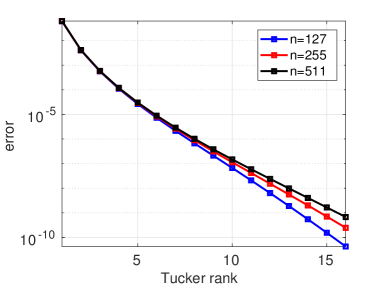
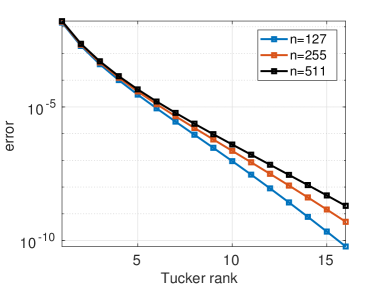
Figure 5.1: Multigrid Tucker approximation of ${\bf G}_{2}$ for $\alpha=1/2$ (left) and $\alpha=1/10$ (right) vs. Tucker rank $r$ for $n\times n\times n$ 3D Cartesian grids with univariate grid size $n=127,\,255,\,511$.

The Tucker core of small size is transformed to a canonical tensor by the Tucker-to-canonical decomposition [31], yielding the mixed tensor format, which is used as the starting rank-structured tensor representation of the governing operator in the solution process. For reducing the Kronecker rank of the system matrix and of the current target vector in the course of the PCG iteration the RHOSVD-based Tucker decomposition to the canonical tensors is applied [31].

6 Numerics on rank-structured tensor numerical schemes

In this section we analyze the rank decomposition of all matrix entities involved in the solution operator (2.10). For the ease of exposition, in what follows, we set the model constants as $\beta=\gamma=1$ and assume that $n_{1}=n_{2}=n_{3}$. Recall that $A=F^{\ast}GF$ with the notation $A=\mathcal{A}_{h}$, where $\mathcal{A}_{h}$ is the FDM approximation to the elliptic operator $\mathcal{A}$ and $G$ is the diagonal core matrix represented in terms of eigenvalues of the discrete Laplacian $A=\mathcal{A}_{h}$. All numerical simulations are performed in MATLAB on a laptop.

First, we illustrate the smoothing properties of the elliptic operator $\mathcal{A}_{h}^{-\alpha}$ in 2D (or by the other words, the localization properties of the fractional operator $\mathcal{A}_{h}^{\alpha}$) in the equation for control depending on the fractional power $\alpha>0$. Figures 6.1, 6.1, 6.3 and 6.4 represent the shape of the design function $y_{\Omega}$ and the corresponding optimal control ${\bf u}^{\ast}$ in the equation (4.4) computed for different values of the parameter $\alpha$ and for fixed grid size $n=255$.

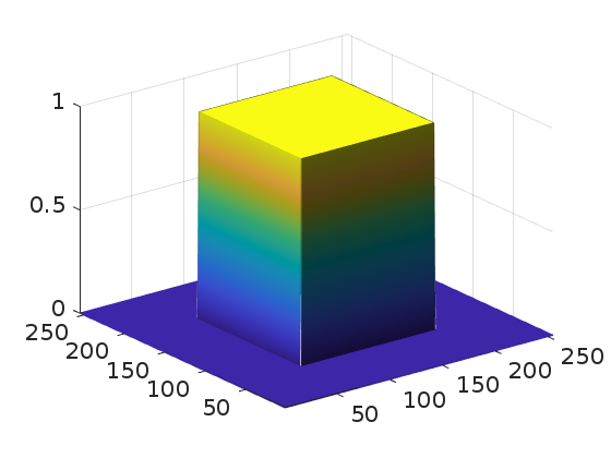
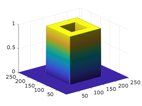
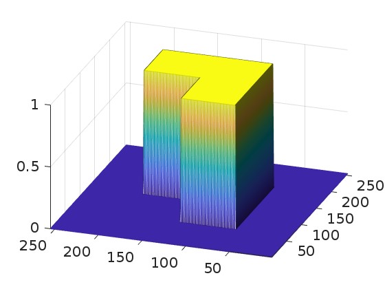
Figure 6.1: Shapes of the right-hand side $y_{\Omega}$ used in the 2D equation (4.4) computed with n=255.

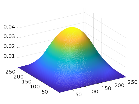
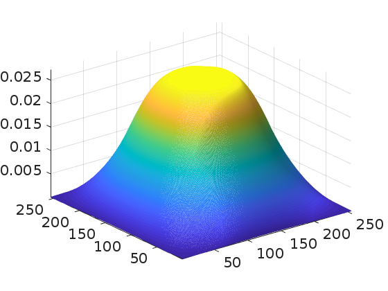
Figure 6.2: Solutions ${\bf u}^{\ast}$ for above right-hand sides $y_{\Omega}$ with $\alpha=1$ for $n=255$.

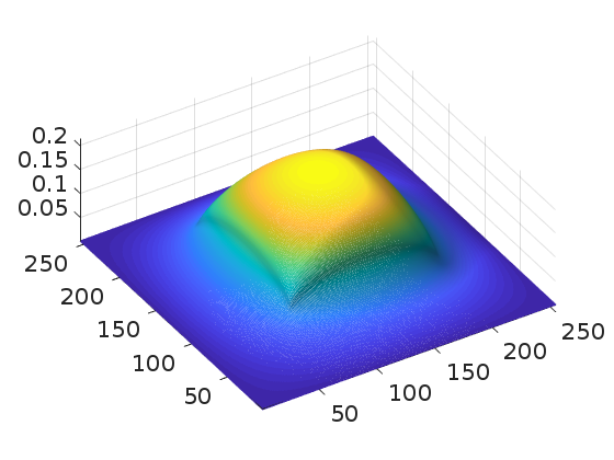
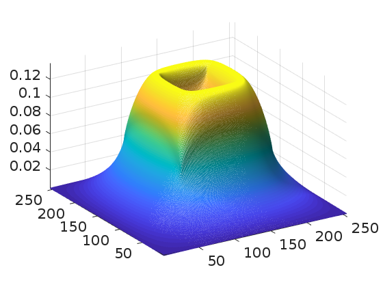
Figure 6.3: Solutions ${\bf u}^{\ast}$ for above right-hand sides with $\alpha=1/2$ for $n=255$.

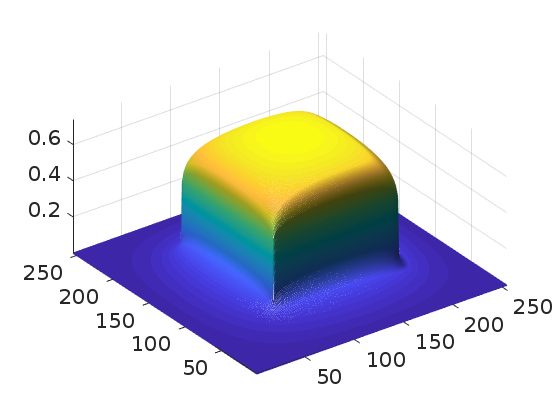
Figure 6.4: Solutions ${\bf u}^{\ast}$ for above right-hand sides with $\alpha=1/10$ for $n=255$.

One observes the nonlocal features of the elliptic resolvent $\mathcal{A}_{h}^{-1}$ and highly localized action of the operator $\mathcal{A}_{h}^{-\frac{1}{10}}$.

6.1 Numerical tests for 2D case

Figure 6.5, left, represents the singular values of the matrix $G_{1}$, with entries given by (4.11) for different univariate grid size $n=255,511$, and $1023$ and fixed $\alpha=1$ (Laplacian inverse). Figure 6.5, right, shows the decay of respective singular values for $G_{1}$ with fixed univariate grid size $n=511$ and for different $\alpha=1,1/2,1/10$.

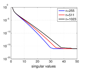
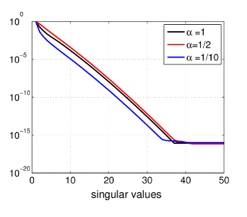
Figure 6.5: Decay of singular values for $G_{1}$ with $\alpha=1$ vs. $n$ (left); singular values for $G_{1}$ vs. $\alpha>0$ with fixed $n=511$ (right).

Figure 6.6 demonstrates the behavior of singular values for matrices $G_{2}$ and $G_{3}$, with the entries corresponding to (4.12) and (4.13), respectively, vs. $\alpha=1,1/2,1/10$ with fixed univariate grids size $n=511$. In all cases we observe exponentially fast decay of the singular values which means there exists the accurate low Kronecker rank approximation of the matrix functions $A_{1},A_{2}$ and $A_{3}$ (see equations (4.1), (4.2) and (4.3)) including fractional powers of the elliptic operator.

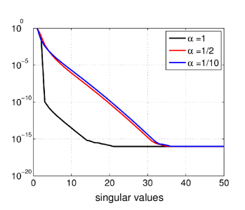
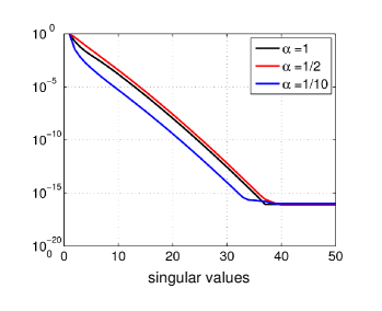
Figure 6.6: Decay of singular values of $G_{2}$ (left) and $G_{3}$ (right) vs. $\alpha=1,1/2,1/10$ for $n=511$.

Decay of the error for the optimal control obtained as the solution of equation (4.4) with rank-$R$ approximation of the solution operator $A_{3}$ is shown in Figure 6.7.

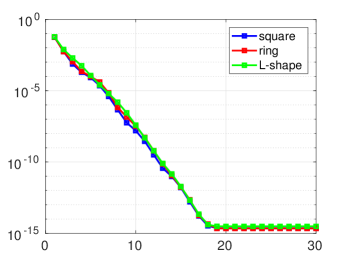
Figure 6.7: Decay of the error for the optimal control vs. truncation rank parameter.

As we have shown theoretically in Section 3, a single PCG iteration has a complexity, which is slightly higher than linear in the univariate grid size $n$. Figure 6.8 shows that the CPU times show the expected behavior. Thus, with Figure 6.8 and Tables 6.1 and 6.2, the overall cost of the algorithm is almost linear in the univariate grid size $n$ for the problem discretized on $n\times n$ 2D Cartesian grid.

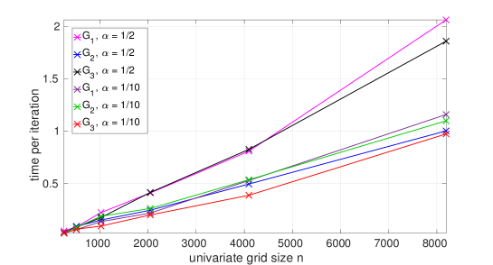
Figure 6.8: CPU times (sec) vs. univariate grid size $n$ for a single iteration of Algorithm 1 for a 2D problem, for different fractional operators and fixed preconditioner rank $r=5$.

We also test the properties of the low-rank discrete operator as a preconditioner. This means, we solve the equations in $\mathbb{R}^{d}$, $d=2,\,3$,

$$A^{\alpha}\mathbf{x} =\mathbf{b},$$ (6.1)

$$\big{(}I+A^{2\alpha}\big{)}\mathbf{x} =\mathbf{b},$$ (6.2)

$$\big{(}A^{\alpha}+A^{-\alpha}\big{)}\mathbf{x} =\mathbf{b},$$ (6.3)

with a preconditioned conjugate gradient scheme, using a low-rank direct solver as a preconditioner discussed above. We simplify the notation by $A={\cal A}_{h}$.

In numerical tests we solve the equations (6.1) - (6.3) on a grid of size $n$, using a rank-$r$ preconditioner. Tables 6.1 and 6.2 show the number of CG iteration counts for convergence to a relative residual of $10^{-6}$ of (6.1)-(6.3) with $\alpha=1/2$ and $\alpha=1/10$, respectively. The dash ‘—’ indicates failure to converge to converge in 100 iterations.

	$g_{1}$				$g_{4}$				$g_{3}$
	256	512	1024	2048	256	512	1024	2048	256	512	1024	2048
1	20	24	24	29	—	—	83	80	20	24	24	19
2	—	—	3	3	73	—	38	36	—	—	3	3
3	7	9	10	14	99	—	17	16	7	9	10	14
4	5	6	6	9	31	—	3	3	5	6	6	9
5	4	4	4	5	11	–	5	5	4	4	4	5
6	3	3	3	4	6	13	2	2	3	3	3	4
7	3	3	3	3	4	7	6	4	3	3	3	3
8	2	2	2	2	3	5	4	2	2	2	2	2
9	2	2	2	2	3	4	3	4	2	2	2	2
10	2	2	2	2	3	3	2	3	2	2	2	2

Table 6.1: PCG iteration counts for convergence to a relative residual of $10^{-6}$ for the equations (6.1) - (6.3) for a 2D fractional Laplacian with $\alpha=1/2$ vs. the univariate grid size $n$ and separation rank $r$.

As can be seen in Tables 6.1 and 6.2, we achieve almost grid-independent preconditioning; the iteration counts only grow logarithmically with the number of grid points, as can be expected from the theoretical reasoning. As can be seen in Table  6.1, the ranks of the preconditioner should be chosen sufficiently large to ensure reliability. In the cases tested here, $r=6$ is sufficient to achieve reliable preconditioning even in the most difficult case of equation (6.2) with $\alpha=1/2$.

	$g_{1}$				$g_{4}$				$g_{3}$
	256	512	1024	2048	256	512	1024	2048	256	512	1024	2048
1	9	9	10	11	11	13	14	16	7	7	8	9
2	6	4	7	8	7	8	8	9	5	5	6	6
3	4	5	5	6	5	5	6	7	4	4	5	5
4	4	4	4	5	4	4	4	5	3	4	4	4
5	3	3	4	4	3	4	4	4	3	3	3	4
6	3	3	3	4	3	3	3	4	2	3	3	3
7	2	3	3	3	2	3	3	3	2	2	3	3
8	2	2	2	3	2	2	2	3	2	2	2	3
9	2	2	2	2	2	2	2	2	2	2	2	3
10	2	2	2	2	2	2	2	2	2	2	2	2

Table 6.2: PCG iteration counts for convergence to a relative residual of $10^{-6}$ for the equations (6.1) - (6.3) for a 2D fractional Laplacian with $\alpha=1/10$ vs. the univariate grid size $n$ and separation rank $r$.

6.2 Numerical tests for 3D case

In the following examples we solve the problems governed by the 3D operators in (4.1) – (4.3), with a 3D fractional Laplacian with $\alpha=1,1/2$ and $\alpha=1/10$. The rank-structured approximation to the above fractional operators is performed by using the multigrid Tucker decomposition of the 3D tensors ${\bf G}_{k}$, $k=1,2,3,4$, described by (4.7) – (4.9), and the consequent Tucker-to-canonical decomposition of the Tucker core tensor thus obtaining a canonical tensor with a smaller rank. The rank truncation procedure in the PCG Algorithm 1 is performed by using the RHOSVD tensor approximation and its consequent transform to the canonical format, see Section 5.

Figures 6.9 – 6.11 demonstrate the exponential convergence of the approximation error with respect to the Tucker rank for operators given by (6.1) – (6.3).

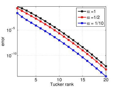
Figure 6.9: Tucker tensor approximation of ${\bf G}_{1}$ vs. rank parameter for $\alpha=1,1/2,1/10$.

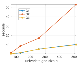
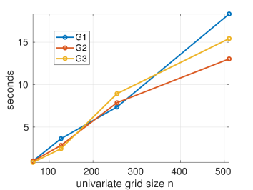
$\alpha=1/2$, $r=4$	$\alpha=1/10$, $r=7$

Figure 6.10: CPU times (in seconds) vs. univariate grid size $n$ for a single iteration of Algorithm 1 for a 3D problem, for different fractional operators and fixed preconditioner rank $r$.

We solve the equations (6.1) - (6.3) using $n\times n\times n$ 3D Cartesian grids with the univariate grid size $n$, using a rank-$r$ preconditioner. Tables 6.3 and 6.4 show the number of CG iteration counts for convergence to a relative residual of $10^{-6}$ of (6.1) - (6.3) with $\alpha=1/2$ and $\alpha=1/10$, respectively.

Similarly to the previous subsection, we see that the low-rank approximation gives us an approximately grid-independent preconditioner. In the cases tested here, $r=6$ is sufficient to achieve reliable preconditioning even in the most difficult case of equation (6.2) with $\alpha=1/2$.

	$g_{1}$				$g_{4}$				$g_{3}$
	64	128	256	512	64	128	256	512	64	128	256	512
4	1	2	1	1	1	6	1	2	1	2	1	1
5	1	1	1	2	1	1	8	4	1	1	1	2
6	1	1	1	1	2	2	1	1	1	1	1	1
7	1	3	1	2	1	1	5	4	1	2	1	2
8	1	1	1	1	1	1	1	1	1	1	1	1
9	1	1	1	2	1	6	5	4	1	1	1	2
10	1	1	1	1	1	6	1	1	1	1	1	1

Table 6.3: PCG iteration counts for convergence to a relative residual of $10^{-6}$ for the equations (6.1) - (6.3) for a 3D fractional Laplacian with $\alpha=1/2$. Here $n$ is the univariate grid size, $r$ is the separation rank.

	$g_{1}$				$g_{4}$				$g_{3}$
	64	128	256	512	64	128	256	512	64	128	256	512
4	2	1	9	20	2	1	10	17	1	1	9	18
5	1	1	1	1	1	1	1	1	1	2	1	13
6	1	1	1	2	1	1	1	2	1	1	1	7
7	1	1	1	2	1	1	1	2	1	1	2	1
8	1	1	1	1	1	1	1	1	1	1	1	2
9	1	1	1	1	1	1	1	1	1	1	1	1
10	1	1	1	2	1	1	1	2	1	1	1	1

Table 6.4: CG iteration counts for convergence to a relative residual of $10^{-6}$ for the equations (6.1)-(6.3) for a 3D fractional Laplacian with $\alpha=1/10$. Here $n$ is the univariate grid size, $r$ is the separation rank.

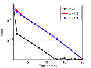
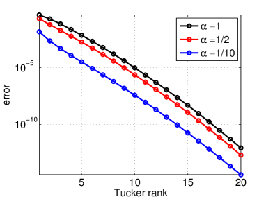
Figure 6.11: Tucker tensor approximation of ${\bf G}_{2}$ and ${\bf G}_{3}$ vs. rank parameter for $\alpha=1,1/2,1/10$.

Our numerical test indicates that all three matrices $A_{1},A_{2}$ and $A_{3}$, as well as the corresponding three-tensors have $\varepsilon$-rank approximation such that the rank parameter depends logarithmically on $\varepsilon$, i.e., $r=O(|\log\varepsilon|)$, that means that the low rank representation of the design function $y_{\Omega}$ ensures the low rank representation of both optimal control and optimal state variable.

We show as well that, using rank-structured tensor methods for the numerical solution of this optimization problem using the operators of type $A_{1},A_{2}$ and $A_{3}$ can be implemented at low cost that scales linearly in the univariate grid size, $O(n\log n)$, see Figure 6.10.

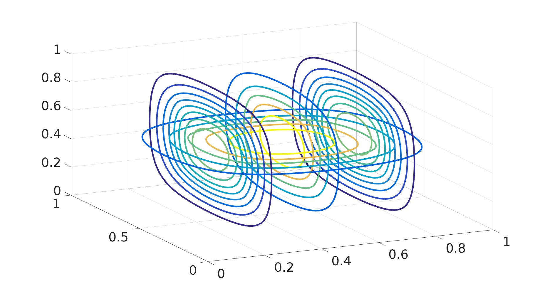
Figure 6.12: Solutions of the equation with 3D right-hand sides (analogous to Figure 6.1) with $\alpha=1$ for $n=255$.

Figure 6.13: Solutions of the equation with 3D right-hand sides (analogous to Figure 6.1) with $\alpha=1/2$ for $n=255$.

Figure 6.14: Solutions of the equation with 3D right-hand sides (analogous to Figure 6.1) with $\alpha=1/10$ for $n=255$.

7 Conclusions

We have introduced and analyzed a new approach for the optimal control of a fractional Laplacian equation using tensor numerical methods. The fractional Laplacian is diagonalized in the FFT basis on a tensor grid and a low Kronecker rank approximation to the core diagonal matrix is computed. We present the novel rank-structured tensor approximation of functions of fractional elliptic operators based on sinc-approximation method. This representation exhibits the exponential decay of the approximation error in the rank parameter.

These results apply to the fractional Laplacian itself, as well as to the solution operators of a fractional control problem, resulting from first-order necessary conditions. Due to the separation of spatial variables in tensor formats, the application of the arising matrix-valued functions of the fractional Laplacian to a given rank-structured vector has a complexity which is nearly linear (linear-logarithmic) in the univariate grid size, independently of the spatial dimension of the problem.

The PCG iterative algorithm with adaptive rank truncation for solving the equation for control function is implemented. In 3D case the rank truncation is based on the RHOSVD-Tucker approximation and its transform to the low-rank canonical form. The numerical study illustrates the exponential decay of the approximation error of the canonical tensor decompositions of the target tensors in the rank parameter, and indicates the almost linear complexity scaling of the rank-truncated PCG solver in the univariate grid size $n$ for 3D problems discretized on $n\times n\times n$ Cartesian grid. The PCG iteration exhibits the uniform convergence rate in the univariate grid size $n$ and other model parameters.

The tensor techniques presented in this paper can be generalized in several directions. First of all, the approach can be extended to the elliptic operators with variable, but well separable, coefficients posed in the box type domains (e.g., layer type or perforated structures), which will be considered elsewhere. Further generalization to the case of non-rectangular domains is also possible. In this case one can use the alternative definition of the fractional elliptic operator by using the Dunford-Cauchy contour integral representation [27, 25, 20] (see (2.9) and related discussion) which is based on computations with the elliptic resolvent in a small number of quadrature points located on the integration path. The practical application of the Dunford-Cauchy representation requires the solution of linear systems of equations involving only the discrete elliptic operator (but not its fractional power). In this case the low-rank tensor decomposition techniques can be applied on domains composed of the moderate number of box type subdomains (e.g., L-shaped, O-shaped or step-type domains).

Finally, we notice that the further reduction of the numerical complexity to the logarithmic scale can be achieved by using the quantized-TT (QTT) representation of all discrete functions and operators involved, see [34, 43, 35].

References

- [1] M. Ainsworth, C. Glusa. Hybrid finite element-spectral method for the fractional Laplacian: approximation theory and efficient solver. SIAM J. Sci. Comput. 40 (4) (2018) A2383-A2405.
- [2] H. Antil and E. Otárola. A FEM for an Optimal Control Problem of Fractional Powers of Elliptic Operators. SIAM J. Control Optim., 53(6), 2015, 3433-3456.
- [3] T.M. Atanackovic, S. Pilipovic, B. Stankovic, and D. Zorica. Fractional Calculus with Applications in Mechanics: Vibrations and Diffusion Processes. John Wiley & Sons, Hoboken, NJ, 2014.
- [4] R. E. Bellman. Dynamic programming. Princeton University Press, 1957.
- [5] A. Bonito, J. P. Borthagaray, R. H. Nochetto, E. Otarola, A. J. Salgado. Numerical methods for fractional diffusion. Computing and Visualization in Science (2018) 1-28.
- [6] L. Banjai, J. M. Melenk, R. H. Nochetto, E. Otárola, A. J. Salgado and Ch. Schwab. Tensor FEM for Spectral Fractional Diffusion. Found. Comput. Math., (2018). https://doi.org/10.1007/s10208-018-9402-3.
- [7] P. Ben-Abdallah, R. Messina, S. Biehs, M. Tschikin, K. Joulain and C. Henkel. Heat Superdiffusion in Plasmonic Nanostructure Networks. Phys. Rev. Lett. 111, 174301, 2013.
- [8] P. Benner. Solving large-scale control problems. IEEE control systems, 24 (1), 2004, pp. 44-59.
- [9] A. Borzi and V. Schulz. Multigrid methods for PDE optimization. SIAM Review 51(2), 2009, 361-395.
- [10] A. Borzi and V. Schulz. Computational optimization of systems governed by partial differential equations. Soc. for Ind. and Appl. Math., Philadelphia, 2012.
- [11] L. Caffarelli and L. Silvestre. An Extension Problem Related to the Fractional Laplacian. Communications in Partial Differential Equations, 32 (8), 2007, pp. 1245-1260.
- [12] A. Cichocki and Sh. Amari. Adaptive Blind Signal and Image Processing: Learning Algorithms and Applications. Wiley, 2002.
- [13] A. Cichocki, N. Lee, I. Oseledets, A. H. Pan, Q. Zhao and D. P. Mandic. Tensor networks for dimensionality reduction and large-scale optimization: Part 1 low-rank tensor decompositions. Foundations and Trends in Machine Learning 9 (4-5), 249-429, 2016.
- [14] L. De Lathauwer, B. De Moor, J. Vandewalle. A multilinear singular value decomposition. SIAM J. Matrix Anal. Appl., 21 (2000) 1253-1278.
- [15] S. Dolgov, D. Kalise, K. Kunisch. A Tensor Decomposition Approach for High-Dimensional Hamilton-Jacobi-Bellman Equations. E-preprint: arXiv:1908.01533, 2019.
- [16] S. Dolgov and I.V. Oseledets. Solution of linear systems and matrix inversion in the TT-format. SIAM J. Sci. Comput. 34 (5), 2011, A2718-A2739.
- [17] S. Dolgov, J. Pearson, D. Savostyanov and M. Stoll. Fast tensor product solvers for optimization problems with fractional differential equations as constraints. Appl. Math. Comp., 273, 2016, 604-623.
- [18] B. Duan, R. Lazarov and J. Pasciak. Numerical approximation of fractional powers of elliptic operators. arXiv:1803.10055v1, 2018.
- [19] I.P. Gavrilyuk, W. Hackbusch, and B. N. Khoromskij. Tensor-product approximation to elliptic and parabolic solution operators in higher dimensions. Computing 74 (2005), 131-157.
- [20] I. P. Gavrilyuk, W. Hackbusch and B. N. Khoromskij. Data-Sparse Approximation to Operator-Valued Functions of Elliptic Operator. Math. Comp. 73, (2003), 1297-1324.
- [21] W. Hackbusch. Tensor spaces and numerical tensor calculus. Springer, Berlin, 2012.
- [22] W. Hackbusch and B.N. Khoromskij. Low-rank Kronecker product approximation to multi-dimensional nonlocal operators. Part I. Separable approximation of multi-variate functions. Computing 76 (2006), 177-202.
- [23] G. Heidel, V. Khoromskaia, B. N. Khoromskij and V. Schulz. Tensor approach to optimal control problems with fractional d-dimensional elliptic operator in constraints. arXiv preprint arXiv:1809.01971, 2018.
- [24] R. Herzog and K. Kunisch. Algorithms for PDE constrained optimization. GAMM, 33 (2010), 163-176.
- [25] Nicholas Hale, Nicholas J Higham, and Lloyd N Trefethen. Computing , , and related matrix functions by contour integrals. SIAM J. on Numerical Analysis, 46 (2), 2008, 2505-2523.
- [26] S. Harizanov, R. Lazarov, P. Marinov, S. Margenov and Ya. Vutov. Optimal solvers for linear systems with fractional powers of sparse spd matrices. Preprint arXiv:1612.04846v3, 2018.
- [27] Nicholas J Higham. Functions of Matrices. SIAM, Philadelphia, 2008.
- [28] M. Hinze, R. Pinnau, M. Ulbrich, and S. Ulbrich. Optimization with PDE Constraints. Math. Model. Theory Appl. 23, Springer, New York, 2009.
- [29] F.L. Hitchcock. The expression of a tensor or a polyadic as a sum of products. J. Math. Physics, 6 (1927), 164-189.
- [30] Karkulik, M., Melenk, J.M. H-matrix approximability of inverses of discretizations of the fractional Laplacian. Adv Comput Math 45, 2893–2919 (2019). https://doi.org/10.1007/s10444-019-09718-5
- [31] Venera Khoromskaia and Boris N. Khoromskij. Tensor Numerical Methods in Quantum Chemistry. De Gruyter Verlag, Berlin, 2018.
- [32] B. N. Khoromskij. Structured Rank- Decomposition of Function-related Tensors in . Comp. Meth. Applied Math., 6, (2006), 2, 194-220.
- [33] B. N. Khoromskij. Tensor-Structured Preconditioners and Approximate Inverse of Elliptic Operators in . Constructive Approximation, 30:599-620 (2009).
- [34] B. N. Khoromskij. -Quantics Approximation of - Tensors in High-Dimensional Numerical Modeling. Constr. Approx., v.34(2), 2011, 257-289.
- [35] Boris N. Khoromskij. Tensor Numerical Methods in Scientific Computing. De Gruyter Verlag, Berlin, 2018.
- [36] B. N. Khoromskij and V. Khoromskaia. Low Rank Tucker-Type Tensor Approximation to Classical Potentials. Central European J. of Math., 5(3), pp.523-550, 2007.
- [37] B. N. Khoromskij and V. Khoromskaia. Multigrid Tensor Approximation of Function Related Arrays. SIAM J. Sci. Comp., 31(4), 3002-3026 (2009).
- [38] B. N. Khoromskij and Ch. Schwab. Tensor-structured Galerkin approximation of parametric and stochastic elliptic PDEs. SIAM J. Sci. Comp., 33 (1), 364-385.
- [39] D. Kressner and C Tobler. Krylov subspace methods for linear systems with tensor product structure. SIAM J Matr. Anal. Appl., 31 (4), 2011, 1688-1714, 2011.
- [40] M. Kwaśnicki. Ten equivalent definitions of the fractional Laplace operator. Functional Calculus and Applied Analysis, 20(1):7-51, 2017.
- [41] A. Lischke, G. Pang, M. Gulian, F. Song, Ch. Glusa, X. Zheng, Z. Mao, W. Cei, M. M. Meerschaert, M. Ainsworth, G. E. Karniadakis. What is the fractional Laplacian? arXiv:1801.09767v1, 2018.
- [42] C. Marcati, M. Rakhuba and C. Schwab. Tensor Rank bounds for Point Singularities in . E-preprint: arXiv:1912.07996, 2019.
- [43] I.V. Oseledets. Approximation of matrices using tensor decomposition. SIAM J. Matrix Anal. Appl., 31(4):2130-2145, 2010.
- [44] I. Podlubny. Fractional Differential Equations. Academic Press. 1999.
- [45] L. S. Pontryagin, V. G. Boltyanskii, R. V. Gamkrelidze, E. F. Mishechenko. The Mathematical Theory of Optimal Processes. Pergamon Press, Oxford, 1964.
- [46] M. R. Rapaić, Z. D. Jelićíć. Optimal control of a class of fractional heat diffusion systems. Nonlinear Dynam. 62 (1-2) 2010, pp. 39-51.
- [47] F. Stenger. Numerical methods based on Sinc and analytic functions. Springer-Verlag, 1993.
- [48] F. Troeltzsch. Optimal control of partial differential equations: theory, methods and applications. AMS, Providence, Rhode Island, 2010.
- [49] L. R. Tucker. Some mathematical notes on three-mode factor analysis. Psychometrika, 31 (1966) 279-311.
- [50] P. N. Vabishchevich. Numerically solving an equation for fractional powers of elliptic operators. J. Comput. Phys., 282, 2015, pp. 289-302.
- [51] P. N. Vabishchevich. Numerical solution of time-dependent problems with fractional power elliptic operator. Comput. Meth. Applied Math., 18 (1), 111-128, 2018.