Classical simulability of noisy boson sampling

Abstract

Quantum mechanics promises computational powers beyond the reach of classical computers. Current technology is on the brink of an experimental demonstration of the superior power of quantum computation compared to classical devices. For such a demonstration to be meaningful, experimental noise must not affect the computational power of the device; this occurs when a classical algorithm can use the noise to simulate the quantum system.

In this work, we demonstrate an algorithm which simulates boson sampling, a quantum advantage demonstration based on many-body quantum interference of indistinguishable bosons, in the presence of optical loss. Finding the level of noise where this approximation becomes efficient lets us map out the maximum level of imperfections at which it is still possible to demonstrate a quantum advantage. We show that current photonic technology falls short of this benchmark. These results call into question the suitability of boson sampling as a quantum advantage demonstration.

In recent years, interest in quantum information processing has focused onto small-scale quantum computing machines, which could perform specific tasks of scientific or technological interest faster than classical computers, and which can be constructed with current or near-future technology Wolf2018 ; Preskill2018 . An important milestone would be demonstrating a quantum device which can convincingly outperform a classical computer at some particular problem, i.e., a demonstration of a quantum advantage Montanaro2017 ; Aaronson2011 . For most quantum advantage proposals, the required system size is predicted to lie around 50 particles/qubits Boixo2018b ; Wusupercomputer ; Pednault2017 , and constructing a quantum system of that size is the current focus of experimental quantum information efforts worldwide Kellly2019 ; Gambetta2019 ; Zhong2018 ; Gong2018 ; Bernien2017 ; Friis2017 .

A major hurdle to experimentally achieve a quantum advantage is our poor understanding of how noise affects the viability of quantum advantage demonstrations Chen2018a ; Boixo2018a ; Boixo2018b ; Bremner2017 ; Markov2018 ; Villalonga2018 ; Gao2018 ; Yung2017 ; Patron2017 ; Oszmaniec2018 ; RahimiKeshari2016 ; Renema2018 ; Shchesnovich2014 ; Arkhipov15 ; Aaronsonweb ; Lund2014 ; Aaronsonlostphotons . Since near-term quantum devices are not error corrected, it is generally believed that they are not scalable to arbitrary size, succumbing to noise for a sufficiently large system size or a sufficiently high level of noise. The challenge lies in finding the point where this occurs for any given system.

The transition from quantum to classical is demarcated by the point at which a classical algorithm can use the inevitably present experimental noise to simulate the task being performed by the quantum system. For such an algorithm to meaningfully restrict the demonstration of a quantum advantage in a given system, it must meet three criteria. First, it must use the types of noise naturally present in the system, at the levels at which they are present in experiments. Second, there must be a well-defined point in terms of system size and noise level where the algorithm becomes efficient; this point then demarcates the level of imperfections admissible in that experiment. Finally, in order for the algorithm to be applicable to near-term devices, the point where the algorithm becomes efficient must lie below the system size being targeted by quantum advantage demonstrations.

In this work, we show an algorithm to classically simulate one quantum advantage platform, namely boson sampling (interference of noninteracting, indistinguishable bosons) Aaronson2011 , in the presence of the two major sources of noise for that experiment, namely particle loss and distinguishability. Our algorithm meets the three criteria outlined above. It efficiently simulates interference of $n$ noisy bosons as polynomially many interference processes of size $k\leq n$, supplemented with $n-k$ classical bosons. Remarkably, $k$ only depends on parameters which quantify the level of noise, and not on the number of particles undergoing interference. This shows that boson sampling at a given level of imperfections only carries the hardness of $k$ interfering bosons, where $k$ acts as an upper bound on the size of a boson sampler that can be constructed in the presence of a given level of noise. Such a $k$ exists for any level of noise, which shows that noisy boson sampling is asymptotically non-scalable. Our results imply that experimental noise defines the maximum size to which a noisy boson sampler can be scaled. Our algorithm is efficient for systems constructed with the best photonic devices currently available.

In boson sampling, the task is to provide samples of the output probability distribution resulting from many-boson interference. Aaronson and Arkhipov Aaronson2011 provided strong complexity-theoretic evidence that this task cannot be simulated efficiently (i.e. in polynomial time) on a classical computer. Boson sampling was initially proposed in the framework of linear quantum optics, but alternative implementations for ion traps IonBS , one-dimensional optical lattices OLBS and superconducting qubits SCBS already exist. Moreover, applications for boson sampling devices have been proposed, particularly in quantum chemistry Huh and machine learning Xanadu . The point where a boson sampler is expected to outperform a supercomputer is around 50 bosons Wusupercomputer , an observation that has spurred a range of experimental efforts Spring2012 ; Broome2012 ; Tillmann2013 ; Crespi2013 ; Bentivegna2015 ; Carolan2015 ; Wang2017 ; Wang2018 ; Zhong2018 .

Progress has also been made on understanding the effect of imperfections on boson sampling. The two main imperfections in boson sampling are photon loss, where some bosons are lost in the course of the experiment, and distinguishability, i.e. bosons having different internal quantum states. Boson sampling with partially distinguishable photons was shown to be classically simulable in Renema2018 . For loss, two sets of results can be singled out. First, boson sampling was shown to retain its hardness Shchesnovich2014 ; Arkhipov15 ; Aaronsonweb ; Lund2014 ; Aaronsonlostphotons for small imperfections, including loss of a constant number of photons (i.e. where the survival probability of each photon goes to one asymptotically). Secondly, boson sampling was shown to be classically simulable when the loss probability increases with the number of photons (i.e. where the per-photon survival probability goes to zero asymptotically) Patron2017 ; Oszmaniec2018 . The experimentally crucial case of a constant surival probability per photon (also known as linear loss) remained unsolved, and was identified as one of the major open problems in boson sampling Aaronsonweb2 ; Aaronsonlostphotons ; Wang2018 .

We demonstrate a classical simulation algorithm for many-body bosonic interference where the per-boson transmission probability $\eta$ is fixed and where the bosons may also have some degree of distinguishability $x$, where $x$ is the internal wavefunction overlap between two arbitrary bosons. We show that for every $x<1$ and $\eta<1$ (i.e. for any level of noise), boson sampling can be approximated as quantum interference of clusters of only $k$ particles. Since $k$ does not depend on the number of bosons $n$, it acts as an upper bound on the size of boson sampler which can be constructed with components of given transmission and bosons with given distinguishability. Since the hardness of a boson sampler is fixed by the number of interfering bosons, and since such an upper bound $k$ exists for any level of noise, boson sampling is asymptotically non-scalable. Our work answers the question of whether boson sampling with linear losses is classically simulable in the affirmative.

We can use our results to estimate the quality of experimental components required to demonstrate a quantum advantage. We find that a transmission of $\eta>0.88$ is necessary to simulate boson sampling with 50 bosons at an accuracy level of 10%, and that the current best boson sampling platforms are restricted to interference of 21 bosons under the same criterion. This shows that achieving a demonstration of a quantum advantage with boson sampling requires more than the construction of high-rate, large-scale photonic systems, as was believed previously Neville2017 : it also requires a qualitative improvement in the equipment used.

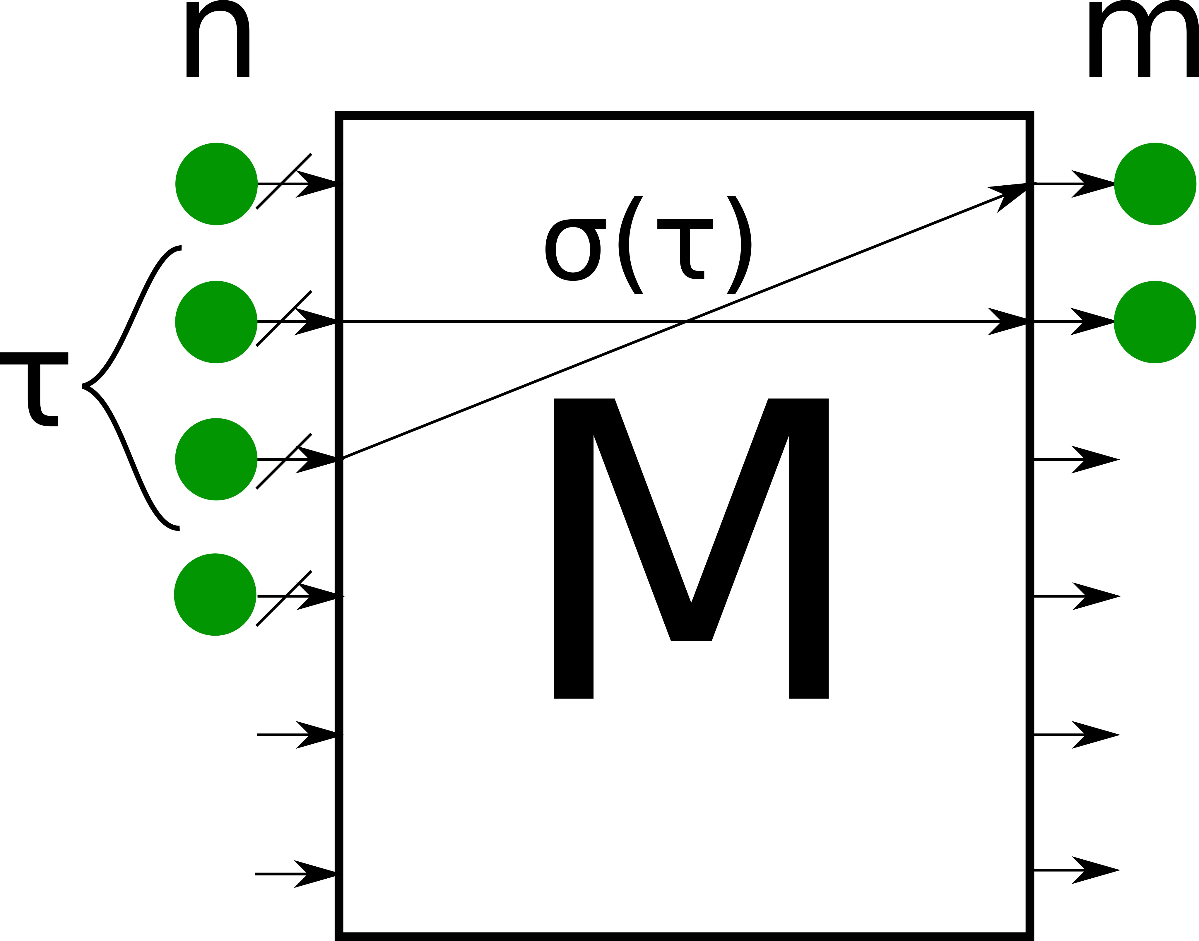
Figure 1: A pictorial representation of a boson sampler with losses. We consider a system with $n$ input particles and $m$ particles at the output, where the particles are lost before they enter the interferometer. The symbols illustrate the notation used in this article: $\tau$ are all ways of selecting $m$ particles from $n$, and $\sigma(\tau)$ are all the ways of permuting those particles. In the figure, we give an example of both.

We begin by setting up the problem, see Figure 1. The initial boson sampling proposal concerns the interference of $n$ single-boson input state over an $N$-mode coupling interferometer modeled by a unitary transformation $U$. At the output we measure the particle number in each mode. A condition for the hardness proof to hold is that the number of modes $N$ obeys $N=O\left(n^{2}\right)$, which guarantees that the probability of two bosons emerging from the same mode (known as a collision) can be neglected. In that case, the probability of the photons exiting the system in a particular set of modes is given by $P=|\mathrm{Perm}(M)|^{2}$ Scheel2008 , where $M$ is a submatrix of the overall unitary transformation $U$ that is chosen by selecting the rows and columns corresponding to the input and output modes respectively, and $\mathrm{Perm}(M)=\sum_{\sigma}\prod_{i}M_{\sigma_{i},i}$ is the permanent function Minc1978 , where $\sigma$ is a permutation and the sum runs over all permutations.

The hardness of boson sampling ultimately stems from the fact that for an arbitrary matrix, the permanent cannot be approximated efficiently by a classical computer Valiant1979 . The best known algorithms for computing an arbitrary permanent are due to Ryser and Glynn Ryser1963 ; Glinn2010 . These algorithms scale as $p2^{p},$ where $p$ is the size of the matrix. It was shown recently Neville2017 that by using a Metropolis algorithm, one can generate samples from a probability distribution where each entry is given by a permanent, at the cost of evaluating a constant number of permanents. The hardness of boson sampling therefore rests on the hardness of computing the individual output probabilities of a boson sampler.

In this paper, we solve how this hardness is compromised by loss and distinguishability. If the losses in each path of the boson sampler are equal, which is a reasonable approximation in experiments, the action of the interferometer is equivalent to a circuit where all losses act at the front of the experiment followed by an ideal interferometer $M$ Neville2017 ; Oszmaniec2018 ; Aaronsonlostphotons . The stochastic nature of the losses will make the number of transmitted photons $m$ fluctuate according to a binomial distribution, but for the purpose of keeping the presentation simple we first present an algorithm for fixed pair $m$ and $n$ and return later to the analysis of the most general case. This scenario fits a recently suggested proposal to circumvent losses in boson sampling by enforcing specific combinations of $n$ and $m$ by post-selecting, as was done recently for $m=5,$ $n=7$ Wang2018 . Our result strongly constrains the viability of this post-selection approach.

To derive our results, we will consider the probability $P$ of an arbitrary collisionless output configuration, without loss of generality. When only $m$ bosons are detected out of the initial $n$, the detection probability at the output results from the incoherent sum over the $\left(\begin{array}[]{c}n\\ m\end{array}\right)$ different ideal boson sampling terms,

$$P={n\choose m}^{-1}\sum_{\tau}|\mathrm{Perm}(M_{\tau})|^{2}={n\choose m}^{-1}\sum_{\tau}P_{\tau},$$ (1)

where $\tau$ is an $m$-combination of $n$ and the sum runs over all such combinations. Each $P_{\tau}$ is the probability corresponding to lossless boson sampling if $m$ bosons were injected in the modes $\tau$. The prefactor ${n\choose m}^{-1}$ arises because of normalization.

Our strategy is to break up equation (1) into terms which correspond to classical transmission, two-boson interference, three-boson interference, and so on. We will then show that boson losses reduce the weight of the higher interference terms. The consequence of this is that beyond some number $k,$ which is only a function of $\eta,$ these terms can be neglected. We can then use our approximation as the input for a Metropolis sampler, which can sample efficiently from our approximate probability distribution.

Our starting point is the following expression for the detection probability in the lossless, fully indistinguishable case Tichypartial :

$$P_{\tau}=|\mathrm{Perm}(M_{\tau})|^{2}=\sum_{\sigma}\mathrm{Perm}(M_{\tau,1}\circ M_{\sigma(\tau),1}^{*}),$$ (2)

where $\sigma$ is a permutation of the elements of $\tau$, the sum runs over all permutations, $\circ$ denotes the elementwise product, ^∗ denotes complex conjugation, and $M_{\sigma,1}$ denotes permuting the rows of matrix $M$ according to $\sigma$ and the columns according to the identity. We will use this notation throughout. For the purpose of keeping the mathematics simple, we shall derive our results for perfect indistinguishability, reintroducing distinguishability at the very end.

Equation 2 can be rewritten by grouping terms according to the number of fixed points (unpermuted elements) in each permutation $\sigma$ Renema2018 . When this is done, permanents of positive matrices arise, which can be approximated efficiently Jerrum2001 . Grouping terms by the size of the derangements $j$ (i.e. the number of elements not corresponding to fixed points) and substituting equation (2) into equation (1), we have:

$$P = {n\choose m}^{-1}\sum_{j=0}^{m}\sum_{\tau}\sum_{\sigma_{j}(\tau)}\sum_{\rho}\mathrm{Perm}(M_{\tau,\rho}\circ M_{\sigma_{j}^{p}(\tau),\rho}^{*})\times$$ (3)

$$\ \ \ \ \ \ \mathrm{\ \ \ \!\ \ \ \ \ \ \ \ \ \ \ \!\ \ \ \ \ \ \ \ \ \ Perm}(|M_{\sigma_{j}^{u}(\tau),\bar{\rho}}|^{2}),$$

where we have made use of their independence to exchange the outer two sums, and where we have used Laplace expansion for permanents to split the matrix permanent into two parts, corresponding to quantum and classical particles, respectively. The notation $\sigma_{j}(\tau)$ denotes a permutation with $m-j$ fixed points which is constructed from the elements of $\tau$, $\sigma_{j}^{p}$ is the permuted part of such a permutation $\sigma_{j},$ $\sigma_{j}^{u}$ is the unpermuted part, $\rho$ is a $j$-combination of $m$, and $\bar{\rho}$ is the complement of that combination. It should be noted that since the size of $\sigma_{j}^{p}$ grows with $j$, the sum over $j$ serves to group terms by computational cost, from easiest to hardest. Simultaneously, one can interpret the $j$-th term as containing all interference processes involving precisely $j$ bosons Rohde2015 .

We show that in equation (3), terms with large $j$ carry less weight and can therefore be neglected beyond some threshold value $k$, which depends on the losses and the desired accuracy of the approximation. Since the $j$-th term represents quantum interference of $j$ bosons, this amounts to showing that boson sampling with losses can be understood as boson sampling of some $k<m$ number of bosons. Therefore, $k$ defines the maximum size of a boson sampler which can be constructed at a given level of losses.

We can formalize this idea by computing the expected value of the $L_{1}$-distance between our approximation $P^{\prime}$ and the exact distribution $P$, i.e., ${d(P,P^{\prime})=\sum_{q}|P(q)-P^{\prime}(q)|},$ where the sum runs over all collision-free outcomes $q$. In the Supplemental Material, we show that at a fixed ratio $\eta=m/n$, the expected value of $d(P,P^{\prime})$ over the ensemble of Haar random unitaries is upper bounded by the expected value of $d(P,P^{\prime})$ as $n$ and $m$ go to infinity while keeping their ratio constant. In that case, the expected value is given by:

$$\mathbb{E}_{U}\left[d(P,P^{\prime})\right]\leq\sqrt{\eta^{k+1}/(1-\eta)}.$$ (4)

We note that since we can only compute the expectation value of the distance, our algorithm will fail for some fraction of unitaries. However, using a standard Markov inequality (see Supplemental Material) one can bound the probability that $d(P,P^{\prime})$ does not satisfy a given bound. If $\mathbb{E}_{U}\left[d(P,P^{\prime})\right]\leq\epsilon$ one can shown that $P\left[d(P,P^{\prime})>\epsilon/\delta\right]$ is upper-bounded by $\delta$. We note that numerical simulations suggest (see Supplemental Material) that the scaling in $\delta$ is actually much better than indicated by this bound.

To use our results for sampling, we use our approximation as the input for a Metropolis sampler that samples efficiently from our approximate probability distribution, which results in a classical simulator of boson sampling with losses. We state the algorithm in full: first, given a value of probability of failure $\delta$, error tolerance $\epsilon$, $n$ and $m$, compute the maximum boson sampler size $k$ using equation (5). Second, randomly choose a set of candidate output modes. Third, compute the approximate output probability by evaluating equation (3) up to the $k$-th term. Fourth, use this probability to compute the acceptance ratio of a Metropolis sampler. Repeat steps 2-4 to generate more samples. In order to compute this approximation, we need evaluate to evaluate a polynomial number of permanents of size up to k Renema2018 .

Solving equation (4) for the maximum boson sampler size $k$ gives the number of bosons beyond which our algorithm becomes efficient, given a user-defined probability of failure $\delta$, error tolerance $\epsilon$ and the value of $\eta$ corresponding to the experimental setup, which scales as

$$k\approx 2\frac{\log\epsilon+\log\delta+\log(1-\eta)}{\log\eta},$$ (5)

which shows that the algorithm is efficient in $\epsilon$ and $\delta$. The fact that $k\rightarrow\infty$ when $\eta\rightarrow 1$, represents the fact that an ideal boson sampler cannot be simulated with our algorithm efficiently, as expected.

We note that equation 5 produces a finite value of $k$ for any level of imperfections $\eta<1$. Therefore, for any level of imperfections, boson sampling can be appoximated as quantum interference of $k<n$ particles and classical interference of the remaining $k-n$ particles. This result shows that demonstrations of a quantum advantage with boson sampling will be non-scalable for any level of imperfections.

However, in practice, one is interested in performing boson sampling at some finite $n$, which should be larger than what can be simulated with a classical supercomputer. Current estimates put this around 50 photons Wusupercomputer . Using these assumptions, the algorithm presented above can be used to rule out a quantum advantage in certain areas of the parameter space. Figure 2 shows the restrictions which our algorithm places on losses: we show parametric plots solving equation (5) for $k$ versus $\eta$, for $\mathbb{E}(d)=0.1,$ $0.01$ and $0.001$. We find that in order to have 50-boson interference while maintaining an average $L_{1}$-distance of $0.1$, a transmission of $\eta>0.88$ is necessary. If a higher accuracy of the classical algorithm is required, this results only in a polynomial increase in $k$.

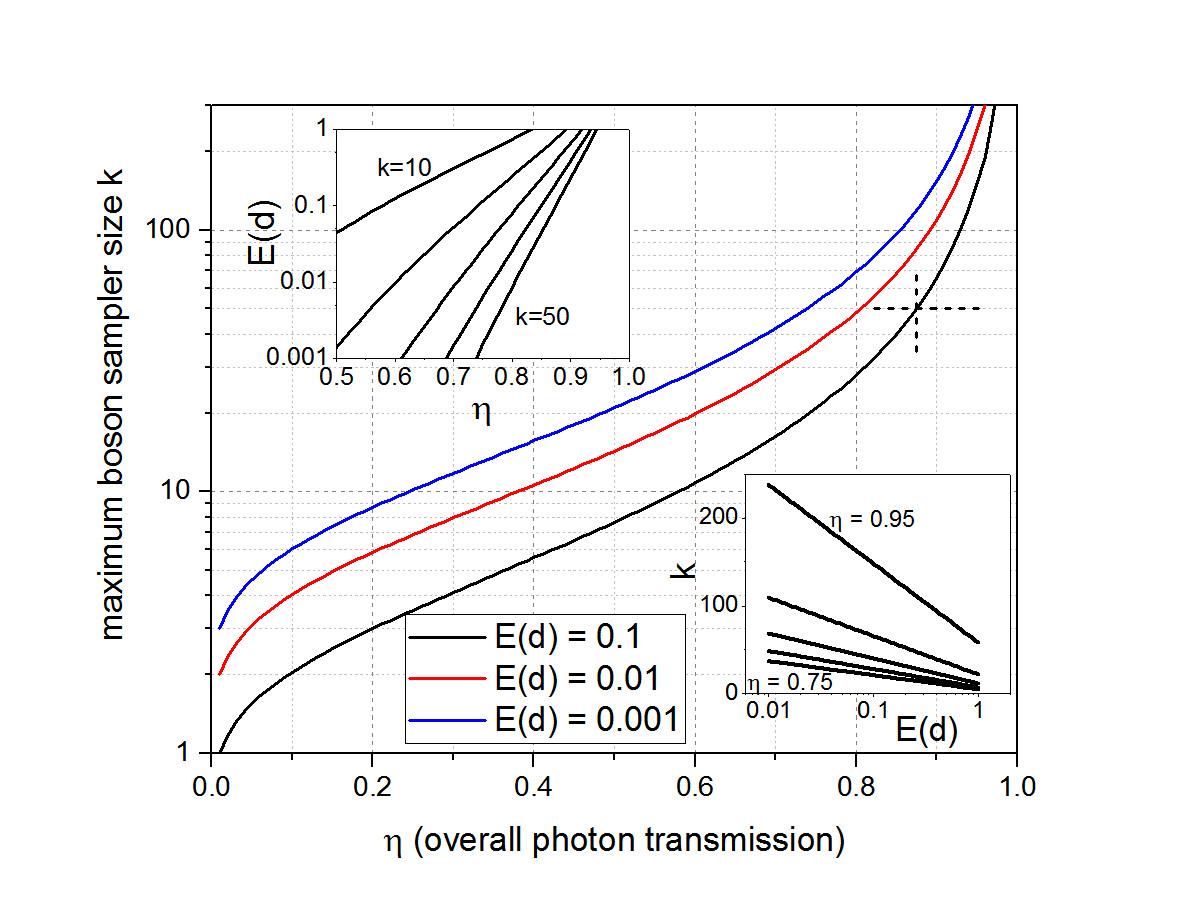
Figure 2: Maximum number of bosons $k$ which can be interfered before our classical algorithm becomes efficient, as a function of the overall boson transmission $\eta,$ including losses in the sources, interferometer and detectors. The horizontal dashed line indicates the point $n=50,$ which is conventionally taken as the limit of a quantum advantage. The vertical dashed line indicates the corresponding requirement of $\eta>0.88$ for $\mathbb{E}(d)=0.1$. Left inset: dependence of $\mathbb{E}(d)$ on $\eta$ for $k=\{10,20,30,40,50\}.$ Right inset: dependence of $k$ on $\mathbb{E}(d)$ for $\eta=\{0.75,0.8,0.85,0.9,0.95\}.$

Losses are not the source of noise that a boson sampling device may suffer from. Experimental partial distinguishability of bosons, which are in principle completely indistinguishable particles, can have an important impact on the quality of an experiment. Following the treatment of Renema2018 , our algorithm leads to a very simple treatment of both sources of noise. We re-introduce a finite level of boson distinguishability, as the overlap $x=\langle\psi_{i}|\psi_{j}\rangle$ for $i\neq j$ of the internal (i.e. non-spatial) parts of the wave function of the photons, where $|\psi_{i}\rangle$ is the internal part of the wave function of the $i$-th boson. As derived in the Supplementary Material, equation (4) holds, but with $\alpha=\eta x^{2}$ taking the place of $\eta.$ Regardless of the specific combination of $\eta$ and $x$ used to achieve it, our algorithm can approximate experiments with equal $\alpha$ equally well. Its value may therefore be taken as a figure of merit of the ability of an experiment to interfere large numbers of bosons.

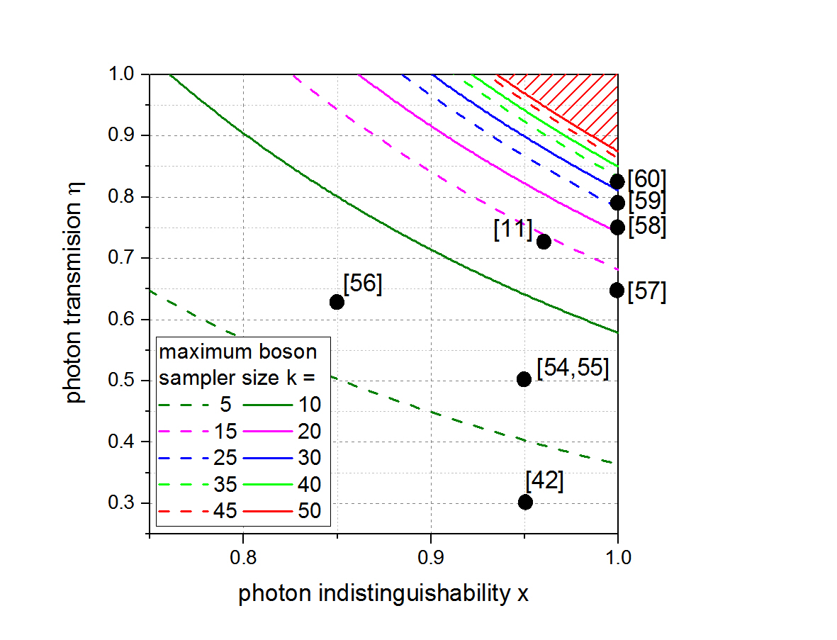
Figure 3: Interchange between distinguishability parameter $x$ and the transmission probability $\eta$, for $\mathbb{E}(d)=0.1$. The lines in this plot are contours of constant $\alpha=\eta x^{2},$ for $\alpha$ corresponding to the number of photons indicated in the legend. The red shaded area in the top right is the region of the parameter space where our algorithm cannot rule out a quantum advantage demonstration. The black points indicate the values of $\eta$ and $x$ of various photon sources reported in the literature.

Figure 3 shows the tradeoff between boson distinguishability and loss. The curves are plots of $\eta=\alpha/x^{2}$, where the $\alpha$ correspond to different values of the maximum boson sampler size $k,$ as indicated in the legend. The black dots incidate various photon sources reported in experiments Wang2017 ; Sparrowquantum ; Quandela ; Gazzano2013 ; Zhong2018 ; Dresdendot ; Shalm2015 ; Giustina2015 ; Slussarenko2017 . The plot was generated for $\mathbb{E}(d)=0.1$. This plot therefore demarcates areas of the parameter space where interference of a given number of photons cannot be simulated at that level of accuracy.

We observe that today, not even the best possible experiments meet the requirements for a scalable demonstration of quantum advantage: considering the best interferometers (99% transmission) Wang2018 , the best detectors (93% efficiency) Marsili2013 and the best photon sources, we arrive at $\alpha=0.755$, which implies that any scalable boson sampling experiments with more than $21$ photons will be simulable with our algorithm at the 10% accuracy level.

In generating Figure 3, the relevant quantity for heralded photon sources (such as those operating on parametric down conversion) is the heralding efficiency, i.e. the probability that a photon enters the experiment given that the source signals that it has produced a photon. The heralding efficiency on parametric down conversion sources can be as high as 82% Slussarenko2017 , but the overall photon generation probability is typically a few percent, to avoid multiphoton generation. While for boson sampling, this does not affect the complexity Lund2014 , further photonic quantum technologies will most likely require photon sources with a high absolute photon generation probability.

Finally, we consider proposals involving postselection on those cases where (almost) all bosons make it through, as is usually done in experiments. Wang et al. recently proposed such an experiment, generating $50+p$ photons and detecting $50$ Wang2018 . Our results show than in such a case (see Supplemental Material), $p\leq 3$ is required in order not to be simulable by our algorithm at the 10% approximation level.

In real experiments, $m$ fluctuates according to a binomial distribution with mean $\eta n$ and variance ${\eta(1-\eta)n}$. One can always efficiently simulate these fluctuations if one has an algorithm for a fixed pair $m$ and $n$, since there are approximately $\sqrt{m}$ possible outcomes which occur with high probability, and these are clustered around $m=\eta n$. As shown in the Supplementary Material, such a postselection only adds a small correction to equation (5) and a prefactor to our bound, which vanishes in the limit of large $n$. Therefore, the classical algorithm starts by estimating a $\tilde{k}$, given a value of probability of failure $\delta$, error tolerance $\epsilon$, and $n$. To generate samples, we simply modify our algorithm to sample over $m$ according to the binomial distribution.

Recently, an estimate of the loss which compromises the demonstration a quantum advantage was given by Neville et al. Neville2017 . Our result improves on this result in several ways. First, we demonstrate how losses induce a transition in the scaling of the runtime of classical simulation of a boson sampler from exponential to polynomial, while their result is essentially a runtime estimate comparing an inefficient classical calculation against an inefficient experiment. Second, because our algorithm is polynomial in the number of particles, the bounds that we find are also much more stringent in an absolute sense. Third, we show that the required transmission is a monotonically increasing function of the number of bosons which is coherently interfered. Whereas Neville2017 was only able to show that lossy boson sampling is at most as hard as regular boson sampling, we show that it is in fact much easier.

Future improvement to this work can by made by generalizing our results to non-uniform losses and more general disitinguishability models and replacing the Metropolis sampler by a direct sampling algorithm, such as the one proposed by Clifford and Clifford Clifford for exact boson sampling. An adaptation of this result to Gaussian boson sampling, an alternative approach for quantum supremacy that has application as a subroutine in a classical-quantum hybrid algorithm for the calculation of the vibronic spectra of molecules and finding dense subgraphs, would also be an interesting future research direction.

In conclusion, we have found an efficient classical simulation algorithm for a quantum advantage proposal, namely boson sampling. This algorithm uses the natural sources of noise present in the system, i.e. linear photon loss and particle distinguishability. It predicts an upper bound to the size of a boson sampler that can be constructed with noisy components. Remarkably, that upper bound only depends on a scale-invariate parameter combining losses and indistinguishability, which allows us to demarcate areas of the parameter space where a quantum advantage is impossible. By evaluating this bound for state-of-the-art photonic components, we find that with current technology, boson sampling cannot demonstrate a quantum advantage.

Author contributions

J.J.R. conceived the work. V.S. and R.G.P. contributed to the proof. All authors contributed to the writing of the manuscript.

Competing interests

The authors declare no competing interests.

References

- (1) R. de Wolf, Ethics Inf. Technol. 19, 271 (2017).
- (2) J. Preskill, arXiv:1801.00862 (2018).
- (3) A.W. Harrow and A. Montanaro, Nature 549 7671, (2017).
- (4) S. Aaronson and A. Arkhipov, Theory Comput. 9, 143 (2013).
- (5) E. Pednault et al., arXiv:1710.05867 (2017).
- (6) S. Boixo et al., Nat. Phys. 14 595-600 (2018).
- (7) J. Wu et al., Nat. Sci. Rev. (2018).
- (8) J. Kelly et al., APS March Meeting 2019, (2019).
- (9) J. Gambetta et al., APS March Meeting 2019, (2019).
- (10) M. Gong et al., arXiv:1811.02292v4, (2018).
- (11) H.-S. Zhong et al., Phys. Rev. Lett. 121, 250505 (2018).
- (12) H. Bernien et al., Nature 551, 579-584, (2017).
- (13) N. Friis et al. Phys. Rev. X 8, 021012, (2018).
- (14) J. Chen, F. Zhang, C. Huang, M. Newman, and Y. Shi, arXiv:1805.01450, (2018).
- (15) S. Boixo, V.N. Smelyanskiy, and H. Neven, arXiv:1708.01875, (2017).
- (16) M. J. Bremner, A. Montanaro, and D. J. Shepherd, Quantum 1, 8 (2017).
- (17) I.L. Markov, A. Fatima, S.V. Isakov, and S. Boixo, arXiv:1807.10749 (2018).
- (18) B. Villalonga et al., arXiv:1811.09599 (2018).
- (19) X. Gao and L. Duan, arXiv:1810.03176 (2018).
- (20) M.-H. Yung and X. Gao, arXiv:1706.08913 (2017).
- (21) J. J. Renema et al., Phys. Rev. Lett. 120, 220502 (2018).
- (22) R. Garcia-Patron, J. J. Renema, and V. Shchesnovich, arXiv:1712.10037 (2017).
- (23) M. Oszmaniec and D. Brod, arXiv:1801.06166 .
- (24) S. Rahimi-Keshari, T. C. Ralph, and C. M. Caves, Phys. Rev. X 6, 021039 (2016).
- (25) V. S. Shchesnovich, Phys. Rev. A 89 (2014).
- (26) A. Arkhipov, Phys. Rev. A 92, 062326 (2015).
- (27) S. Aaronson, Scattershot bosonsampling: a new approach to scalable bosonsampling experiments https://www.scottaaronson.com/blog/?p=1579.
- (28) A. P. Lund et al., Phys. Rev. Lett. 113, 100502 (2014).
- (29) S. Aaronson and D. J. Brod, Phys. Rev. A 93, 012335 (2016).
- (30) C. Shen, Z. Zhang, and L.-M. Duan, Phys. Rev. Lett. 112, 050504 (2014).
- (31) G. Muraleedharan, A. Miyake, and I. H. Deutsch, arXiv:1805.01858v2 (2018).
- (32) S. Goldstein et al., Phys. Rev. B 95, 020502(R) (2017).
- (33) J. Huh et al., Nat. Photon. 9, 9 615-620 (2015).
- (34) S. Lloyd and C. Weedbrook, Phys. Rev. Lett. 121, 040502 (2018).
- (35) J. B. Spring et al., Science 339, 798 (2012).
- (36) M. A. Broome et al., Science 339, 794 (2012).
- (37) M. Tillmann et al., Nat. Photon. 7, 540 (2013).
- (38) A. Crespi et al., Nat. Photon. 7, 545 (2013).
- (39) M. Bentivegna et al., Sci. Adv. 1, e1400255 (2015).
- (40) J. Carolan et al., Science 349, 711 (2015).
- (41) H. Wang et al., Nat. Photon. 11, 361 (2017).
- (42) H. Wang et al., Phys. Rev. Lett. 120, 230502 (2018).
- (43) S. Aaronson, Introducing some british people to p vs. np (comment 84) https://www.scottaaronson.com/blog/?p=2408.
- (44) A. Neville et al., Nat. Phys. 13, 1153 (2017).
- (45) S. Scheel, Acta Phys. Slovaca 58, 675 (2008).
- (46) H. Minc, Permanents, Encyclopedia of Mathematics and its Applications. 6. (Addison-Wesley, 1978).
- (47) L. Valiant, Theor. Comput. Sci. 8, 189 (1979).
- (48) H. J. Ryser, Combinatorial Mathematics (Mathematical Association of America, 1963).
- (49) D. Glynn, Eur. J. Comb. 31, 1887 (2010).
- (50) M. C. Tichy, Phys. Rev. A 91, 022316 (2015).
- (51) M. Jerrum, A. Sinclair, and E. Vigoda, A polynomial-time approximation algorithm for the permanent of a matrix with non-negative entries (ACM Press, 2001).
- (52) P. P. Rohde, Phys. Rev. A 91, 012307 (2015).
- (53) An implementation of this algorithm can be found online at https://github.com/jrenema/BosonSampling
- (54) Sparrow quantum application note, http://sparrowquantum.com/wp-content/uploads/2017/12/multiphotonapplicationnote.pdf.
- (55) Quandela edelight-r specifications http://quandela.com/edelight.
- (56) O. Gazzano et al., Nat. Commun. 4, 1425 (2013).
- (57) Y. Chen. et al., Nat. Commun. 9, 2994 (2018).
- (58) L. K. Shalm et al., Phys. Rev. Lett. 115, 250402 (2015).
- (59) M. Giustina et al., Phys. Rev. Lett. 115, 250401 (2015).
- (60) S. Slussarenko et al., Nat. Photon 11, 700 (2017).
- (61) F. Marsili et al., Nat. Photon 7, 210 (2013).
- (62) P. Clifford and R. Clifford, arXiv:1706.01260 (2017).