Elimination of spurious modes within QRPA

Abstract

We suggest a generalized method for elimination of spurious admixtures (SA) from intrinsic nuclear excitations described within the Quasiparticle-Random-Phase-Approximation (QRPA). Various kinds of SA-corrections are treated at the same theoretical ground. The known corrections are well reproduced. As relevant cases, we consider subtraction of SA related with i) violation of the translational invariance (isovector $E1$ and isoscalar toroidal and compression $E1$ modes), ii) pairing-induced non-conservation of the particle number $(E2(K=0)$ and $E0$ modes), and iii) rotational invariance $(E2(K=1)$ and $M1(K=1)$ modes). The SA subtraction can be done at the level of QRPA states, electromagnetic responses, and even transition operators. The additional deformation-induced corrections for $E1$ excitations are proposed and shown to be essential for the compression isoscalar mode. The accuracy of the method is demonstrated by Skyrme QRPA calculations for axially-deformed ¹⁵⁴Sm.

I Introduction and motivation

Theoretical analysis of intrinsic nuclear excitations is often complicated by presence of spurious modes Th61 ; TV62 ; Mar69 ; Row70 ; Ri80 ; BR86 . These modes appear in the intrinsic spectra if some symmetries (translational, rotational) and corresponding conservation laws (for the total momentum ${\bf P}$ and angular momentum ${\bf J}$) are violated by the intrinsic Hamiltonian. The spurious modes of this kind represent the motion of the whole nucleus (translation, rotation) in the laboratory frame. They are obviously beyond the intrinsic nuclear dynamics and so have to be removed from the intrinsic spectra. Another particular case is the pairing-induced non-conservation of the proton and neutron numbers, when the nuclear wave function is contaminated by admixtures from neighbouring nuclei.

Usually the intrinsic Hamiltonian breaks the conservation laws in its mean field and pairing parts. There are many ways for subtraction of emergent spurious admixtures (SA). For example, in $E1$ isovector responses, SA are removed using the proper effective charges Ri80 . In the second-order E1 toroidal and compression isoscalar responses, SA are eliminated by corrections in the transition operators, requiring the nuclear center-of-mass to be in rest VG81 ; Ha01 ; Ba94 ; Kv11 . There is also a diversity of projection techniques to exclude SA, e.g. Ri80 ; Be03 ; Ni06 ; RRR18 ; Co00 ; Ju08 ; Na07 ; Mi12 ; Ars10 .

Random Phase Approximation (RPA) and its quasiparticle version (QRPA) are now widely used for the self-consistent description of giant resonances and low-energy states in spherical and deformed nuclei, see e.g. Kv11 ; Be03 ; Co00 ; Ju08 ; Ars10 ; Na07 ; Mi12 ; Re92 ; Vre00PLB ; Vre02tor ; Pa07 ; Kl08 ; Kv16E0 ; Te10 ; Ne16E2 . As was shown by Thouless Th61 , RPA has a principle ability to separate exactly spurious and physical states. In this method, the spurious mode appears as RPA eigenstate with zero energy, which guaranties orthogonality of the spurious and physical states. Various aspects of this RPA (QRPA) feature are described in detail elsewhere, see e.g. TV62 ; Mar69 ; Row70 ; Ri80 ; Be03 ; BR86 ; KvNa86 ; Na17 .

This RPA advantage to exclude SA was used in early studies within schematic models where violated symmetries were restored by the proper choice of the residual interaction compensating the contamination of the mean field Pya77 . However this scheme is not relevant for the modern self-consistent RPA methods (Skyrme, Gogny, relativistic) where the RPA residual interaction is already fully determined by the initial density functional. Another technique, also not self-consistent, offers additional terms in the RPA residual interaction to shift the spurious modes outside the energy region of interest Pa67 ; Do05 .

In fully self-consistent RPA (QRPA) models with a complete configuration space, the spurious modes have to be entirely located at zero-energy eigenstates. However, even in modern self-consistent RPA calculations this is usually not the case, see e.g. discussion in Be03 ; Pa07 . Due to a limited size of configuration space and numerical inaccuracy, we are almost never able to put the spurious state exactly to the zero energy: its energy is usually a small positive value. Then the spurious mode is not orthogonal to physical states and contaminates them, at least neighboring ones. So the problem of SA persists even in modern self-consistent models.

In the present paper, we propose a simple general method for elimination of SA from QRPA states and electromagnetic responses. The method allows to extract arbitrary (related to different symmetries) SA in the framework of one and the same scheme. We partly use the idea Ju08 ; Co00 ; Na07 ; Mi12 to refine QRPA physical states requiring their orthogonality to the spurious mode. However, in our study, this idea is realized in a general way using basic QRPA properties. Our scheme allows to remove SA not only from QRPA wave functions but also directly from electromagnetic responses, e.g. by correcting transition operators. Our amendments to $E1$ responses reproduce well known effective charges and corrections obtained by various prescriptions Ri80 ; Ha01 . Moreover, we derive and test for these responses the additional deformation-induced SA-corrections.

In general, the method can be applied to both spherical and deformed nuclei. We present the formalism and numerical illustrations obtained within the self-consistent Skyrme QRPA. The main relevant cases are considered: violation of the translational and rotational invariance and pairing-induced non-conservation of the particle number. New analytical deformation-induced corrections for SA-elimination from E1 excitations are derived and tested.

The paper is organized as follows. In Section II, the QRPA background and detailed description of the method are presented. In Section III, we demonstrate and discuss examples of SA elimination from $E1$, $E0$, $E2$, and $M1$ excitations in the axially deformed nucleus ¹⁵⁴Sm. In Sec. IV, the conclusions are done.

II Theoretical framework

II.1 QRPA equations

In this subsection, we sketch the basics of QRPA formalism Ri80 used below in derivation and analysis. We consider even-even axially-deformed nuclei with the states characterized by quantum numbers $K^{\pi}$, where $K$ is the component of the angular momentum to the symmetry axis $z$ and $\pi$ is the space parity. For nuclear interaction of multipolarity $\lambda\mu$, we have $K=\mu\geq$0 with $\pi=(-1)^{\lambda}$ for electric and $\pi=(-1)^{\lambda+1}$ for magnetic modes.

The intrinsic body-fixed Hamiltonian reads

$$\hat{H}_{\rm intr}=\hat{H}_{\rm BCS}+\hat{V}_{\rm res}$$ (1)

where $\hat{H}_{\rm BCS}$ describes mean field and pairing, $\hat{V}_{\rm res}$ is the residual interaction.

One-phonon QRPA eigenstates $Q^{\dagger}_{\nu}|0\rangle$ (with $|0\rangle$ being the QRPA vacuum) are described by the phonon creation operator

$$\hat{Q}^{\dagger}_{\nu}=\sum_{i>j}\;\big{(}X^{(\nu)}_{ij}\alpha^{+}_{i}\alpha^{+}_{j}-Y^{(\nu)}_{ij}\alpha_{\bar{j}}^{\phantom{*}}\alpha_{\bar{i}}^{\phantom{*}}\big{)}$$ (2)

defined as a superposition of $\mathcal{N}$ two-quasiparticle (2qp) $ij$-excitations with quantum numbers $\mu^{\pi}$. The pairs $ij$ with $K_{i}+K_{j}=\mu$ and $i\bar{j}$ with $K_{i}-K_{j}=\mu$ are used. The condition $i>j$ means that we involve configurations with $K_{i}\geq K_{j}>0$; $\nu$ numerates the phonons with given $\mu^{\pi}$; $X^{(\nu)}_{ij}$ and $Y^{(\nu)}_{ij}$ are forward and backward 2qp amplitudes; $|\bar{i}\rangle=\mathcal{T}|i\rangle$ are time-reversed states. The time-reversed counterpart of (2) reads

$$\hat{Q}^{\dagger}_{\bar{\nu}}=\>\sum_{i>j}\big{(}X^{(\nu)*}_{ij}\alpha^{+}_{\bar{i}}\alpha^{+}_{\bar{j}}-Y^{(\nu)*}_{ij}\alpha_{j}\alpha_{i}\big{)}\>.$$ (3)

The phonon operators obey the features

$$\hat{J}_{3}\hat{Q}^{\dagger}_{\nu}|0\rangle=\mu\hat{Q}^{\dagger}_{\nu}|0\rangle,\;\hat{J}_{3}Q^{\dagger}_{\bar{\nu}}|0\rangle=-\mu\hat{Q}^{\dagger}_{\bar{\nu}}|0\rangle$$ (4)

where $\hat{J}_{3}$ is z-component of the total momentum $\hat{\bf{J}}$.

Amplitudes $X^{(\nu)}_{ij}$ and $Y^{(\nu)}_{ij}$ and phonon energies $\hbar\omega_{\nu}$ are obtained from QRPA equations of motion:

$$[\,\hat{H}_{\rm intr},\>\hat{Q}^{\dagger}_{\nu}\,] =\hbar\omega_{\nu}\>\hat{Q}^{\dagger}_{\nu}\>,$$ (5a)

$$[\,\hat{H}_{\rm intr},\>\hat{Q}_{\nu}\,] =-\hbar\omega_{\nu}\>\hat{Q}_{\nu}\>,$$ (5b)

$$[\,\hat{Q}_{\nu},\>\hat{Q}^{\dagger}_{\nu^{{}^{\prime}}}\,] =\delta_{\nu\nu^{{}^{\prime}}}.$$ (5c)

In the matrix form, these equations read Ri80

$$\begin{pmatrix}A&B\\ B&A\end{pmatrix}\begin{pmatrix}X^{(\nu)}\\ Y^{(\nu)}\end{pmatrix}=\hbar\omega_{\nu}\>\begin{pmatrix}X^{(\nu)}\\ -Y^{(\nu)}\end{pmatrix}.$$ (6)

They include real matrices $A$ and $B$:

$$A_{ij\,i^{{}^{\prime}}\!j^{{}^{\prime}}} \equiv(E_{i}+E_{j})\,\delta_{ij,\,i^{{}^{\prime}}\!j^{{}^{\prime}}}$$

$$\quad{}+\langle\rm{BCS}|\,\big{[}\alpha_{j}\,\alpha_{i},\>[\hat{V}_{res},\,\alpha^{+}_{i^{{}^{\prime}}}\alpha^{+}_{j^{{}^{\prime}}}]\big{]}\,|\rm{BCS}\rangle\>,$$ (7a)

$$B_{ij\>i^{{}^{\prime}}\!j^{{}^{\prime}}} \equiv-\langle\rm{BCS}|\,\big{[}\alpha_{j}\,\alpha_{i},\,[\hat{V}_{res},\,\alpha_{\bar{j}^{{}^{\prime}}}\alpha_{\bar{i}^{{}^{\prime}}}]\big{]}\,|\rm{BCS}\rangle$$ (7b)

(where $|\rm{BCS}\rangle$ is BCS vacuum) and one-column matrices

$$X^{(\nu)}\equiv\begin{pmatrix}\vdots\\ X^{(\nu)}_{ij}\\ \vdots\end{pmatrix}\qquad Y^{(\nu)}\equiv\begin{pmatrix}\vdots\\ Y^{(\nu)}_{ij}\\ \vdots\end{pmatrix}\quad ij=1,\cdots,\mathcal{N}\>.$$ (8)

According to our time-reversal convention for one-body operators $\hat{A}$,

$$\mathcal{T}^{-1}\hat{A}\mathcal{T}=\gamma_{\mathcal{T}}^{A}\hat{A}^{\dagger}\quad\Rightarrow$$

$$\langle i|\hat{A}|j\rangle=\gamma_{\mathcal{T}}^{A}\langle\bar{j}|\hat{A}|\bar{i}\rangle,\quad\langle i|\hat{A}|\bar{j}\rangle=-\gamma_{\mathcal{T}}^{A}\langle j|\hat{A}|\bar{i}\rangle\>,$$ (9)

we introduce time-even ($\gamma_{\mathcal{T}}^{A}=+1$) and time-odd ($\gamma_{\mathcal{T}}^{A}=-1$) operators. Then, instead of the phonon creation and annihilation operators, one may define the generalized time-even coordinate and time-odd momentum operators

$$\hat{\mathcal{X}}_{\nu}=\sum_{i>j}\mathcal{X}^{(\nu)}_{ij}(\alpha^{+}_{i}\alpha^{+}_{j}+\alpha_{\bar{j}}\alpha_{\bar{i}})\;,$$ (10a)

$$\hat{\mathcal{P}}_{\nu}=\sum_{i>j}\mathcal{P}^{(\nu)}_{ij}(\alpha^{+}_{i}\alpha^{+}_{j}-\alpha_{\bar{j}}\alpha_{\bar{i}})\;.$$ (10b)

Following (9), their time-reversed conjugates are

$$\hat{\mathcal{X}}_{\bar{\nu}}^{\phantom{\dagger}}\equiv\hat{\mathcal{X}}_{\nu}^{\dagger},\quad\hat{\mathcal{P}}_{\bar{\nu}}^{\phantom{\dagger}}\equiv-\hat{\mathcal{P}}_{\nu}^{\dagger},$$ (11a)

$$\mathcal{X}^{(\bar{\nu})}_{\bar{i}\bar{j}}=\mathcal{X}^{(\nu)*}_{ij},\quad\mathcal{P}^{(\bar{\nu})}_{\bar{i}\bar{j}}=\mathcal{P}^{(\nu)*}_{ij}.$$ (11b)

Operators $\hat{\mathcal{X}}_{\nu}$ and $\hat{\mathcal{P}}_{\nu}$ are related to the phonon operators (2)-(3) as

$$\hat{\mathcal{X}}_{\nu} =\sqrt{\frac{\hbar}{M_{\nu}\omega_{\nu}}}\frac{1}{\sqrt{2}}\>\big{(}\hat{Q}_{\bar{\nu}}+\hat{Q}^{\dagger}_{\nu}\big{)}\>,$$ (12a)

$$\hat{\mathcal{P}}_{\nu} =\frac{\hbar}{i}\>\sqrt{\frac{M_{\nu}\omega_{\nu}}{\hbar}}\frac{1}{\sqrt{2}}\>\big{(}\hat{Q}_{\bar{\nu}}-\hat{Q}^{\dagger}_{\nu}\big{)}$$ (12b)

and vice versa,

$$\hat{Q}^{\dagger}_{\nu} =\sqrt{\frac{M_{\nu}\omega_{\nu}}{2\hbar}}\hat{\mathcal{X}}_{\nu}-\frac{i}{\sqrt{2\hbar M_{\nu}\omega_{\nu}}}\hat{\mathcal{P}}_{\nu}\>,$$ (13a)

$$\hat{Q}_{\bar{\nu}} =\sqrt{\frac{M_{\nu}\omega_{\nu}}{2\hbar}}\hat{\mathcal{X}}_{\nu}+\frac{i}{\sqrt{2\hbar M_{\nu}\omega_{\nu}}}\hat{\mathcal{P}}_{\nu}\;.$$ (13b)

The orthonormalization condition is

$$\big{[}\,\hat{\mathcal{X}}_{\nu},\>\hat{\mathcal{P}}_{\nu^{\prime}}^{\dagger}\,\big{]}=-2\>\sum_{i>j}\mathcal{X}^{(\nu)}_{ij}\mathcal{P}^{(\nu^{\prime})*}_{ij}=i\hbar\delta_{\nu\nu^{{}^{\prime}}}\;.$$ (14)

If $\mathcal{X}^{(\nu)}_{ij}$ is real, then $\mathcal{P}^{(\nu)}_{ij}$ is imaginary, and vice versa. Following (12)-(14), operators $\hat{\mathcal{X}}_{\nu}$ and $\hat{\mathcal{P}}_{\nu}$ are defined up to an arbitrary factor $M_{\nu}$ which cannot be fixed by the normalization condition.

The QRPA equations (5) can be expressed in terms of $\hat{\mathcal{X}}_{\nu}$ and $\hat{\mathcal{P}}_{\nu}$ as

$$\big{[}\,\hat{H}_{\rm{intr}},\,\hat{\mathcal{P}}_{\nu}\,\big{]} =i\hbar M_{\nu}\omega^{2}_{\nu}\,\hat{\mathcal{X}}_{\nu}\;,$$ (15a)

$$\big{[}\,\hat{H}_{\rm{intr}},\,\hat{\mathcal{X}}_{\nu}\,\big{]} =-\frac{i\hbar}{M_{\nu}}\>\hat{\mathcal{P}}_{\nu}\;,$$ (15b)

$$\big{[}\,\hat{\mathcal{X}}_{\nu},\,\hat{\mathcal{P}}_{\nu^{\prime}}^{\dagger}\,\big{]} =i\hbar\>\delta_{\nu\nu^{{}^{\prime}}}$$ (15c)

or, in the matrix form, as

$$\begin{pmatrix}A&B\\ B&A\end{pmatrix}\begin{pmatrix}\mathcal{P}^{(\nu)}\\ \mathcal{P}^{(\nu)}\end{pmatrix} =i\hbar M_{\nu}\omega^{2}_{\nu}\>\begin{pmatrix}\mathcal{X}^{(\nu)}\\ \mathcal{X}^{(\nu)}\end{pmatrix}\;,$$ (16a)

$$\begin{pmatrix}A&B\\ B&A\end{pmatrix}\begin{pmatrix}\mathcal{X}^{(\nu)}\\ -\mathcal{X}^{(\nu)}\end{pmatrix} =\frac{\hbar}{i}\frac{1}{M_{\nu}}\>\begin{pmatrix}\mathcal{P}^{(\nu)}\\ -\mathcal{P}^{(\nu)}\end{pmatrix}\;,$$ (16b)

where, in analogy with (8), $\mathcal{X}^{(\nu)}$ and $\mathcal{P}^{(\nu)}$ are one-column matrices for 2qp amplitudes of the generalized coordinate and momentum. For given $K^{\pi}$, the intrinsic Hamiltonian (1) in terms $\hat{\mathcal{X}}_{\nu}$ and $\hat{\mathcal{P}}_{\nu}$ has the form

$$\hat{H}_{\rm intr}\approx\hat{H}_{\rm QRPA}=\sum_{\nu}\!\bigg{(}\frac{\hat{\mathcal{P}}_{\nu}\hat{\mathcal{P}}_{\nu}^{\dagger}}{2M_{\nu}}+\frac{1}{2}M_{\nu}\omega^{2}_{\nu}\,\hat{\mathcal{X}}_{\nu}\hat{\mathcal{X}}_{\nu}^{\dagger}\bigg{)}\;.$$ (17)

This expression shows that the parameter $M_{\nu}$ can be treated as an inertia (mass) value for each QRPA state.

Note that $\langle\hat{\mathcal{X}},\hat{\mathcal{P}}\rangle$-presentation can be fruitful for construction of modern self-consistent QRPA versions based on the functionals with time-even and time-odd densities and currents Re92 , see particular cases of Skyrme QRPA in Ne02 ; Ne06 .

II.2 Extraction of spurious admixtures

The invariance of the Hamiltonian $\hat{H}_{\rm intr}$ under translation or rotation of the whole nucleus leads to the conservation condition

$$\big{[}\,\hat{H}_{\rm intr},\,\hat{P}\,\big{]}=0$$ (18)

where $\hat{P}$ is the corresponding time-odd transformation generator. The motion of the whole nucleus contaminates the intrinsic nuclear excitations and leads to SA which have to be extracted from the intrinsic spectra. For the translation, generator $\hat{P}$ is the linear momentum operator of the whole nucleus. In axial deformed nuclei, the center-of-mass translation contaminates the intrinsic $K^{\pi}=0^{-}$ and $1^{-}$ states. For the rotation, $\hat{P}$ is the total angular momentum operator. The rotation pollutes intrinsic $K^{\pi}=1^{+}$ states.

Following Th61 ; TV62 , just $\langle\hat{\mathcal{X}},\hat{\mathcal{P}}\rangle$-presentation of QRPA is suitable for the treatment of spurious modes. Indeed, it is easy to see that the first equation from QRPA set (15) reproduces condition (18) if $\omega_{0}=0$ and generator $\hat{P}$ is identified with QRPA generalized momentum $\hat{\mathcal{P}}_{0}$. Then the Hamiltonian (17) recasts to

$$\hat{H}_{\rm QRPA}=\frac{\hat{\mathcal{P}}_{0}\hat{\mathcal{P}}_{0}^{\dagger}}{2M_{0}}+\sum_{\nu>0}\!\bigg{(}\frac{\hat{\mathcal{P}}_{\nu}\hat{\mathcal{P}}_{\nu}^{\dagger}}{2M_{\nu}}+\frac{1}{2}M_{\nu}\omega^{2}_{\nu}\,\hat{\mathcal{X}}_{\nu}\hat{\mathcal{X}}_{\nu}^{\dagger}\bigg{)}$$ (19)

where the spurious $\nu=0$ state with $\omega_{0}=0$ yields the first term Ri80 . The generalized coordinate $\hat{\mathcal{X}}_{0}$ is obtained from Eq. (15b) for given $\hat{\mathcal{P}}_{0}$. Note that $\hat{\mathcal{X}}_{0}$ is absent in (19). The spaces $\{\hat{\mathcal{X}}_{0},\hat{\mathcal{P}}_{0},\hat{\mathcal{X}}_{\nu>0},\hat{\mathcal{P}}_{\nu>0}\}$ and $\{\hat{\mathcal{X}}_{0},\hat{\mathcal{P}}_{0},\hat{Q}^{\dagger}_{\nu>0},\hat{Q}_{\nu>0}\}$ constitute the complete sets of QRPA states. The condition $\omega_{0}=0$ obviously hampers the construction of well-normalized spurious (s) phonon operator

$$\hat{Q}^{\dagger}_{s}\equiv x_{s}\>\hat{\mathcal{X}}_{0}-\frac{i}{2\hbar\>x_{s}}\>\hat{\mathcal{P}}_{0}$$ (20)

with $x_{s}=\sqrt{M_{0}\>\omega_{0}/(2\hbar)}$. So the exact spurious eigenstate can be defined in terms of $\hat{\mathcal{X}}_{0}$ and $\hat{\mathcal{P}}_{0}$ but not in the phonon representation.

In addition to (18), one may also consider the conservation law for the particle number,

$$[\,\hat{H}_{\rm intr},\,\hat{N}_{q}\,]=0\;,$$ (21)

where $\hat{N}_{q}$ is the time-even particle-number operator for protons ($q=p$) or neutrons ($q=n$). Violation of this law results in spurious admixtures in $K^{\pi}=0^{+}$ states. The condition (21) is held by the QRPA equation (15b) if a) $\hat{N}$ is identified with the QRPA generalized coordinate $\hat{\mathcal{X}}_{0}$ and b) we apply $M_{0}\to{+}\infty$ and $\omega_{0}\to 0$ while keeping $M_{0}\omega_{0}^{2}$ finite (though this can be hardly realized in practice).

As mentioned in the Introduction, in self-consistent QRPA calculations we are almost never able to put the energy of the first eigenstate precisely to zero. Even very large 2qp basis is usually not enough to get $\omega_{0}=0$. As a result, the conservation laws (18) and (21) are not held precisely and the spurious mode, though being mainly concentrated in the lowest $\nu=0$ state, still contaminates the neighbouring physical states with $\nu>0$. In other words, the exact spurious mode and states with $\nu>0$ are not orthogonal.

Let’s suppose that we have almost pure spurious state $|\nu^{\prime}=0\rangle$ whose energy $\delta\omega_{0}$ is yet not zero but a tiny positive value. This state is a reasonable approximation to the exact spurious mode, i.e. $|\nu^{\prime}=0\rangle\approx|s\rangle$. What is important for our aims, the state $|\nu^{\prime}=0\rangle$ with $\delta\omega_{0}>0$ may be normalized,

$$\big{[}\,\hat{\mathcal{X}}_{0},\>\hat{\mathcal{P}}_{0}^{\dagger}\,\big{]}=i\hbar\;,$$ (22)

and presented in the phonon form (20).

Let’s further suppose that we have QRPA self-consistent states $|\nu\rangle$ contaminated by SA. Our goal is to refine these states from SA. This can be done requiring orthogonality of the refined states $|\nu^{\prime}>0\rangle$ to the spurious mode $|s\rangle$ approximated by (20):

$$\langle\nu^{\prime}|s\rangle=\langle 0|\,\big{[}\hat{Q}_{\nu^{\prime}},\hat{Q}^{\dagger}_{s}\big{]}\,|0\rangle=0$$ (23)

The phonon operator for $|\nu^{\prime}\rangle=\hat{Q}^{\dagger}_{\nu^{\prime}}|0\rangle$ is searched in the form

$$\hat{Q}^{\dagger}_{\nu^{\prime}}=\hat{Q}^{\dagger}_{\nu}-\alpha_{\nu}\hat{\mathcal{P}}_{0}-\beta_{\nu}\hat{\mathcal{X}}_{0}$$ (24)

where $\alpha_{\nu}$ and $\beta_{\nu}$ should be defined from the condition (23). This prescription reminds the projection methods used in some previous studies for particular spurious modes, see e.g. Co00 ; Ju08 ; Ars10 ; Na07 ; Mi12 . However, as compared with Co00 ; Ju08 ; Ars10 , we use a more general expression (20) for the spurious state where both $\hat{\mathcal{X}}_{0}$ and $\hat{\mathcal{P}}_{0}$ operators are included. As shown below, our way allows to derive a more general scheme for SA-elimination. There are also essential differences from Na07 ; Mi12 , see discussion in Sec. IV.D.

The condition (23) gives

$$\alpha_{\nu}=\bigg{[}\frac{\langle 0|\,\big{[}\hat{Q}_{\nu},\,\hat{\mathcal{X}}_{0}\big{]}\,|0\rangle}{\langle 0|\,\big{[}\hat{\mathcal{P}}^{\dagger}_{0},\,\hat{\mathcal{X}}_{0}\big{]}\,|0\rangle}\bigg{]}^{*}\;,\beta_{\nu}=\bigg{[}\frac{\langle 0|\,\big{[}\hat{Q}_{\nu},\,\hat{\mathcal{P}}_{0}\big{]}\,|0\rangle}{\langle 0|\,\big{[}\hat{\mathcal{X}}^{\dagger}_{0},\,\hat{\mathcal{P}}_{0}\big{]}\,|0\rangle}\bigg{]}^{*}$$ (25)

or, using (22),

$$\alpha_{\nu}=\frac{1}{i\hbar}\langle 0|\,\big{[}\hat{Q}_{\nu},\,\hat{\mathcal{X}}_{0}\big{]}\,|0\rangle^{*},\;\beta_{\nu}=\frac{i}{\hbar}\langle 0|\,\big{[}\hat{Q}_{\nu},\,\hat{\mathcal{P}}_{0}\big{]}\,|0\rangle^{*}.$$ (26)

It is easy to check that

$$\langle 0|\,\big{[}\hat{Q}_{\nu^{\prime}},\,\hat{\mathcal{X}}_{0}\big{]}\,|0\rangle=\langle 0|\,\big{[}\hat{Q}_{\nu^{\prime}},\,\hat{\mathcal{P}}_{0}\big{]}\,|0\rangle=0$$ (27)

i.e., within the quasiboson approximation, the refined physical states are indeed orthogonal to the generators $\hat{\mathcal{P}}_{0}$ and $\hat{\mathcal{X}}_{0}$ and so to the spurious state (20). In this derivation, we use the feature that average commutator of operators with the definite time parity,

$$\langle 0|\,[\hat{A},\,\hat{B}]\,|0\rangle\propto(1-\gamma_{\mathcal{T}}^{A}\gamma_{\mathcal{T}}^{B})\;,$$ (28)

vanishes if operators $\hat{A}$ and $\hat{B}$ have the same time parity $(\gamma_{\mathcal{T}}^{A}=\gamma_{\mathcal{T}}^{B}$) in the sense (9).

Note that result (27) does not depend on the concrete values of $x_{s}$, $M_{\nu}$ and $\omega_{0}$. For determination of $\alpha_{\nu}$ and $\beta_{\nu}$, we should know the symmetry operator and its conjugate, i.e. $\hat{\mathcal{P}}_{0}$ and $\hat{\mathcal{X}}_{0}$. These operators are given below in Sec. III for all the cases of interest.

The above scheme allows to refine QRPA states. However in practice we often need a direct refinement of the transition matrix elements and responses. This can be done within our approach as well. Let’s consider the matrix element of the transition operator $\hat{\mathcal{M}}$ between the physical refined state $|\nu^{\prime}\rangle$ and RPA vacuum:

$$\langle\nu^{\prime}|\,\hat{\mathcal{M}}\,|0\rangle =\langle 0|\,[\hat{Q}_{\nu^{\prime}},\hat{\mathcal{M}}]\,|0\rangle=\langle 0|\,\big{[}\hat{Q}_{\nu},\,\hat{\mathcal{M}}\big{]}\,|0\rangle$$ (29)

$$-\alpha_{\nu}^{*}\langle 0|\,\big{[}\hat{\mathcal{P}}^{\dagger}_{0},\,\hat{\mathcal{M}}\big{]}\,|0\rangle-\beta_{\nu}^{*}\langle 0|\,\big{[}\hat{\mathcal{X}}^{\dagger}_{0},\,\hat{\mathcal{M}}\big{]}\,|0\rangle\,.$$

Using the feature (28) it is easy to see that, depending on the time parity of $\hat{\mathcal{M}}$, the second (third) term in (29) vanishes at $\gamma_{\mathcal{T}}^{\mathcal{M}}=-1$ ( $\gamma_{\mathcal{T}}^{\mathcal{M}}=1$). Then we get

$$\langle\nu^{\prime}|\hat{\mathcal{M}}|0\rangle=\langle\nu|\hat{\mathcal{M}}|0\rangle-\frac{i}{\hbar}\langle\nu|\hat{\mathcal{X}}_{0}|0\rangle\langle 0|[\hat{\mathcal{P}}_{0}^{\dagger},\hat{\mathcal{M}}]|0\rangle$$ (30)

for time-even $\hat{\mathcal{M}}$ and

$$\langle\nu^{\prime}|\hat{\mathcal{M}}|0\rangle=\langle\nu|\hat{\mathcal{M}}|0\rangle+\frac{i}{\hbar}\langle\nu|\hat{\mathcal{P}}_{0}|0\rangle\langle 0|[\hat{\mathcal{X}}_{0}^{\dagger},\hat{\mathcal{M}}]|0\rangle$$ (31)

for time-odd $\hat{\mathcal{M}}$. Expressions (30)-(31) can be used for calculation of the refined transition matrix elements.

Using (30)-(31), the refined transition densities and currents read:

$$\delta\rho_{\nu^{\prime}}(\bf{r}) = \delta\rho_{\nu}({\bf r})-\frac{i}{\hbar}\langle 0|[Q_{\nu},\hat{\mathcal{X}}_{0}^{\dagger}]|0\rangle\langle 0|[\hat{\mathcal{P}}_{0}^{\dagger},\hat{\rho}({\bf r})]|0\rangle,$$ (32)

$$\delta{\bf j}_{\nu^{\prime}}({\bf r}) = \delta{\bf j}_{\nu}({\bf r})+\frac{i}{\hbar}\langle 0|[Q_{\nu},\hat{\mathcal{P}}_{0}^{\dagger}]|0\rangle\langle 0|[\hat{\mathcal{X}}_{0}^{\dagger},\hat{\bf{j}}({\bf r})]|0\rangle,$$ (33)

where the density and current operators are defined in Appendix A.

One may go further and reduce SA-elimination to modification of transition operators. Indeed expressions (30)-(31) can be rewritten as $\langle\nu^{\prime}|\hat{\mathcal{M}}|0\rangle=\langle\nu|\hat{\tilde{\mathcal{M}}}|0\rangle$ with

$$\hat{\tilde{\mathcal{M}}} = \hat{\mathcal{M}}-\frac{i}{\hbar}\langle 0|[\hat{\mathcal{P}}_{0}^{\dagger},\hat{\mathcal{M}}]|0\rangle\hat{\mathcal{X}}_{0}\quad\text{for}\;\gamma_{\mathcal{T}}^{\mathcal{M}}=1,$$ (34)

$$\hat{\tilde{\mathcal{M}}} = \hat{\mathcal{M}}+\frac{i}{\hbar}\langle 0|[\hat{\mathcal{X}}_{0}^{\dagger},\hat{\mathcal{M}}]|0\rangle\hat{\mathcal{P}}_{0}\quad\text{for}\;\gamma_{\mathcal{T}}^{\mathcal{M}}=-1.$$ (35)

Expressions (34)-(35) suggest the simplest way for elimination of SA from the responses. They lead to the important conclusion that QRPA in principle allows to refine responses through modification of transition operators. As compared with building of the refined QRPA states (24), expressions (30)-(35) suggest more economical elimination prescriptions with usage of initial QRPA states $|\nu\rangle$.

Note that there is an alternative way to obtain expressions (34)-(35). Since physical and spurious QRPA solutions form the complete basis, any operator linear in the boson approximation can be expressed as Mar69 ; Row70 ; Ser03

$$\hat{\mathcal{M}} = \sum_{\nu>0}\bigg{(}\langle 0|[\hat{\mathcal{Q}}_{\nu},\hat{\mathcal{M}}]|0\rangle\hat{\mathcal{Q}}^{\dagger}_{\nu}-\langle 0|[\hat{\mathcal{Q}}_{\nu}^{\dagger},\hat{\mathcal{M}}]|0\rangle\hat{\mathcal{Q}}_{\nu}\bigg{)}$$ (36)

$$+ \frac{i}{\hbar}\bigg{(}\langle 0|[\hat{\mathcal{P}}_{0}^{\dagger},\hat{\mathcal{M}}]|0\rangle\hat{\mathcal{X}}_{0}-\langle 0|[\hat{\mathcal{X}}_{0}^{\dagger},\hat{\mathcal{M}}]|0\rangle\hat{\mathcal{P}}_{0}\bigg{)}$$

where last two terms are spurious contributions. Removal of these contribution just gives (34)-(35). This correspondence can be treated as the additional check of the validity of our projection procedure (23)-(24). Note that our procedure is more comprehensive than direct usage of (36) since it allows to refine not only operators and their matrix elements but also QRPA wave functions.

Expressions (30)–(35) do not include the factor $x_{s}$. However they need the knowledge of the spurious operators $\hat{\mathcal{P}}_{0}$ and $\hat{\mathcal{X}}_{0}$. As shown in Sec. 4, in some cases, e.g. for $E1$ excitations, both the symmetry operator and its conjugate are known, and SA corrections acquire a simple analytical form. If not, then 2qp amplitudes of the unknown conjugate and the parameter $M_{0}$ can be determined from equations Ri80

$$\mathcal{X}^{(0)}_{ij} =\frac{\hbar}{i}\frac{1}{M_{0}}\sum_{kl}\big{(}A-B\big{)}^{-1}_{ij,\,kl}\,\mathcal{P}^{(0)}_{kl},$$ (37)

$$M_{0} =2\!\sum_{i>j,\,k>l}\mathcal{P}^{(0)*}_{ij}\,\big{(}A-B\big{)}^{-1}_{ij,\,kl}\,\mathcal{P}^{(0)}_{kl}$$ (38)

or

$$\mathcal{P}^{(0)}_{ij} =i\hbar\omega_{\nu}^{2}M_{0}\sum_{kl}\big{(}A+B\big{)}^{-1}_{ij,\,kl}\,\mathcal{X}^{(0)}_{kl},$$ (39)

$$M_{0} =\frac{1}{2\omega_{\nu}^{2}}\,\bigg{\{}\sum_{i>j,\,k>l}\mathcal{X}^{(0)}_{ij}\big{(}A+B\big{)}^{-1}_{ij,\>kl}\,\mathcal{X}^{(0)*}_{kl}\>\bigg{\}}^{-1}.$$ (40)

As shown in Appendix B, the averages $\langle 0|[....]|0\rangle$ in (30)-(35) are directly calculated through $\mathcal{P}^{(0)}_{ij}$, $\mathcal{X}^{(0)}_{ij}$ and transition matrix elements.

III Details of calculations

The calculations for axially deformed ¹⁵⁴Sm are performed within QRPA approach with the Skyrme forces Re92 ; Be03 ; Rep17EPJA . The total functional includes the Skyrme, Coulomb and pairing terms. Our approach is fully self-consistent since both mean field and residual interaction are derived from the initial functional, using all the available densities and currents. The Coulomb contribution includes direct and exchange terms in Slater approximation. The volume pairing is treated at the BCS level. Both particle-hole and pairing-induced particle-particle channels are involved Rep17EPJA . More detail on the approach are given in the Appendix C. Implementation of the approach to the code is described in Re15th ; Re15ar .

We use Skyrme parameterization SLy6 Cha98 which was found successful in our previous QRPA calculations for various dipole excitations Kv11 ; Kl08 ; Ne02 ; Ne06 ; Kv13 ; Rep17EPJA ; NePRL18 ; Ne18ar . Hartree-Fock (HF) mean field is computed using 2D grid in cylindrical coordinates (with mesh size 0.4 fm and calculation box of about three nuclear radii). The single-particle space embraces all the levels from the bottom of the potential well up to 40 MeV (1533 proton and 1722 neutron levels in ¹⁵⁴Sm). The volume pairing is treated at the BCS level. The equilibrium quadrupole deformation $\beta=0.339$ is obtained by minimization of the system energy. QRPA calculations use a large two-quasiparticle (2qp) basis. For example, for $K^{\pi}=1^{-}$ states, the basis includes $\approx$ 9000 proton and $\approx$ 16000 neutron quasiparticle pairs. The Thomas-Reiche-Kuhn sum rule Ri80 and isoscalar dipole energy-weighted sum rule Ha01 are exhausted by 95$\%$ and 97$\%$, respectively.

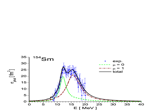
Figure 1: The total QRPA photoabsorption cross section (black solid curve) and its $\mu=0$ and $\mu=1$ branches (green dashed and black dashed-dotted curves) as compared with the experimental data Gu81 .

Strength function for $X\lambda\mu$-transitions between the ground state $|0\rangle$ and QRPA states $|\nu\rangle$ reads

$$S_{k}(X\lambda\mu;\,E)=\sum_{\nu}(\hbar\omega_{\nu})^{k}\big{|}\,\langle\nu|\hat{\mathcal{M}}_{X\lambda\mu}|0\rangle\,\big{|}^{2}\,\delta_{\Delta}(E-\hbar\omega_{\nu})$$ (41)

where $X=E,M$ marks electric and magnetic cases, $\hbar\omega_{\nu}$ is the excitation energy of $\nu$-state, $\langle\nu|\,\hat{\mathcal{M}}_{X\lambda\mu}|0\rangle$ is the transition matrix element. Components $\mu\neq$ 0 embrace both $+\mu$ and $-\mu$ contributions. Further

$$\delta_{\Delta}(E-\hbar\omega_{\nu})=\frac{1}{2\pi}\>\frac{\Delta(\hbar\omega_{\nu})}{(E-\hbar\omega_{\nu})^{2}+[\Delta(\hbar\omega_{\nu})/2]^{2}}$$ (42)

is the Lorentz weight simulating smoothing effects beyond QRPA (escape width and coupling to complex configurations). To simulate a general growth of the smoothing with the excitation energy, the energy-dependent folding parameter is used Kv13 :

$$\Delta(\hbar\omega_{\nu})=\begin{cases}\Delta_{0}&\text{for }\hbar\omega_{\nu}\leq E_{0}\\[2.0pt] \Delta_{0}+a\,(\hbar\omega_{\nu}-E_{0})&\text{for }\hbar\omega_{\nu}>E_{0},\end{cases}$$ (43)

where the values $\Delta_{0}$, $a$, and $E_{0}$ are adjusted to describe the experimental photoabsorption cross section. For ¹⁵⁴Sm, these values are $\Delta_{0}=0.1$ MeV, $a=0.15$, and $E_{0}=8.3$ MeV. Then the calculated photoabsorption cross section

$$\sigma_{\rm phot}(E)=\frac{16\pi^{3}}{137\cdot 9\,e^{2}}\sum_{\mu=0,\pm 1}S_{1}(E1\mu;\,E)$$ (44)

well reproduces the experimental data Gu81 , see Fig. 1. Here the ordinary effective charges $e^{\rm eff}_{p}=N/A$ and $e^{\rm eff}_{p}=-Z/A$ are used. In the next section, these charges are derived in the framework of our SA-elimination method.

Being comfortable for description of the high-energy photoabsorption, the particular energy-dependent folding (42) with the small low-energy averaging $\Delta_{0}=0.1$ MeV is generally not convenient for illustration of SA-elimination in various low-energy excitations. So, in the next section, we use the folding with the larger constant averaging $\Delta_{0}=0.4$ MeV.

IV Results and Discussion

In this section, we apply our SA-elimination method to the following particular cases: 1) violation of the translational invariance ($K^{\pi}=0^{-}$ and $1^{-}$ states; ordinary, toroidal (tor) and compression (com) $E1K$ transitions), 2) pairing induced non-conservation of the particle number ($K^{\pi}=0^{+}$ states; $E0$ and $E20$ transitions), 3) violation of the rotational invariance ($K^{\pi}=1^{+}$ states; $E21$ and $M11$ transitions).

We show in subsection IV.1 that elimination of SA from ordinary, compression and toroidal $E1$ responses is reduced to simple corrections in the transition operators. Just this simplest way is used in numerical calculations. In the cases of non-conservation of the particle number (subsection IV.2) and violation of the rotational invariance (subsection IV.3), the building of simple SA-corrections is hampered. So, in these cases, the numerical results are obtained by formation of the refined QRPA states (24). Namely, using the known symmetry operator and relations (37)-(40), the set of $\mathcal{P}^{(0)}_{ij}$ and $\mathcal{X}^{(0)}_{ij}$ is obtained. Then, following (91), the averages $\langle 0|\,\big{[}Q_{\nu},\,\hat{\mathcal{M}}\big{]}\,|0\rangle$ are calculated and coefficients $\alpha_{\nu}$ and $\beta_{\nu}$ are determined to construct finally the refined state.

IV.1 $E1$ transitions

IV.1.1 Ordinary E1 transitions in the long-wave limit

The center-of-mass (CoM) translation of the whole nucleus can lead to SA in intrinsic dipole nuclear states $K^{\pi}=0^{-}$ and $1^{-}$ . For $\mu=K$, the operator of CoM linear momentum is

$$\hat{\mathcal{P}}_{0[\mu]}=-i\hbar\sum_{k=1}^{A}(\nabla_{\mu})_{k}$$ (45)

where $\mu=0,\pm 1$, $\nabla_{0}=\frac{\partial}{\partial z}$ , $\nabla_{\pm 1}=\mp\frac{1}{\sqrt{2}}\>(\frac{\partial}{\partial x}\pm i\frac{\partial}{\partial y})$, $\nabla^{\dagger}_{\mu}=(-1)^{\mu+1}\nabla_{-\mu}$. Then, subject to the normalization condition $[\,\hat{\mathcal{X}}_{0[\mu]},\,\hat{\mathcal{P}}_{0[\mu]}^{\dagger}\,]=i\hbar$, the CoM coordinate operator has the form

$$\hat{\mathcal{X}}_{0[\mu]}=\sqrt{\frac{4\pi}{3}}\frac{1}{A}\sum_{k=1}^{A}(rY_{1\mu}(\hat{r}))_{k}\;.$$ (46)

The operators (45) and (46) can be obviously treated as QRPA operators constituting the spurious state (20). This state has the inertia parameter $M_{0}=mA$ and fully exhausts the energy-weighted sum rule $EWSR=\frac{3\hbar^{2}}{8\pi m}A$ for isoscalar long-wave dipole excitations.

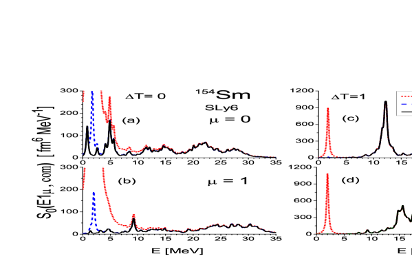
Figure 2: The QRPA compression $E1$ strength function (41) in ¹⁵⁴Sm calculated with the parametrization SLy6. The isoscalar (left panels) and isovector (right panels) strengths are considered. The branches $\mu=0$ (top), $\mu=1$ (bottom) are plotted for the polluted strength ”no elim” (red dotted curves) and refined strengths ”sph elim” and ”full elim”, calculated without (blue dash curve) and with (black solid curves) deformation correction $d^{\mu}_{q}$, respectively.

Now let’s consider the proton transition dipole operator in the long-wave limit:

$$\hat{\mathcal{M}}_{E1\mu}=\sum_{k=1}^{Z}(rY_{1\mu})_{k}.$$ (47)

Following (34), this time-even operator is refined as

$$\hat{\tilde{\mathcal{M}}}_{E1\mu}=\hat{\mathcal{M}}_{E1\mu}-\frac{i}{\hbar}\langle 0|[\hat{P}^{\dagger}_{0[\mu]},\hat{\mathcal{M}}_{E1\mu}]|0\rangle\hat{X}_{0[\mu]}.$$ (48)

Using the relation $[\hat{P}^{\dagger}_{0[\mu]},\hat{\mathcal{M}}_{E1\mu}]=-i\hbar Z\sqrt{\frac{3}{4\pi}}$ and Eq. (46) for $\hat{X}_{0[\mu]}$, the above expression is reduced to

$$\hat{\tilde{\mathcal{M}}}_{E1\mu} = \sum_{k=1}^{Z}(rY_{1\mu})_{k}-\frac{Z}{A}\sum_{k=1}^{A}(rY_{1\mu})_{k}$$ (49)

$$= \frac{N}{A}\sum_{k=1}^{Z}(rY_{1\mu})_{k}-\frac{Z}{A}\sum_{k=1}^{N}(rY_{1\mu})_{k}.$$

So, for $E1\mu$-transitions, we get the standard effective charges $e^{\rm eff}_{p}=N/A$ and $e_{n}^{\rm eff}=-Z/A$, This justifies validity of our method in this particular case. The dipole strength function obtained with this effective charges is demonstrated in Fig. 1.

IV.1.2 Compression E1 transitions

The transition operator for $E1$ compression mode (CM) is Ha01

$$\hat{\mathcal{M}}_{E1\mu,\rm{com}}^{(\Delta T)}=\frac{1}{10}\sum_{q=n,p}e^{(\Delta T)}_{q}\sum_{k\in q}(r^{3}Y_{1\mu})_{k}\;.$$ (50)

The effective charges are

$$e^{(\Delta T)}_{p} = e^{(\Delta T)}_{n}=1\quad\text{for isoscalar case}\quad\Delta T=0,$$ (51)

$$e^{(\Delta T)}_{p} = -e^{(\Delta T)}_{n}=1\quad\text{for isovector case}\quad\Delta T=1.$$

Usually CM is observed in the isoscalar reaction $(\alpha,\alpha^{\prime})$ Ha01 , so the channel $\Delta T$=0 is most relevant. However, for the completeness, we also consider the case $\Delta T$=1. Operator (50) originates from the second-order term in the long-wave decomposition of the total electric $E1$ transition operator, see Kv11 for more detail. $E1$ compression mode can be affected by CoM motion. The spurious QRPA momentum (45) and coordinate (46) operators are obviously the same as for ordinary $E1$ transitions considered above.

Since the transition operator (50) is time-even, its refined version is determined by Eq. (34):

$$\hat{\tilde{\mathcal{M}}}^{(\Delta T)}_{E1\mu,\rm{com}} = \hat{\mathcal{M}}^{(\Delta T)}_{E1\mu,\rm{com}}$$

$$- \frac{i}{\hbar}\langle 0|[\hat{P}^{\dagger}_{0[\mu]},\hat{\mathcal{M}}^{(\Delta T)}_{E1\mu,\rm{com}}]|0\rangle\hat{X}_{0[\mu]}.$$

Using relations (97)-(99) for vector spherical harmonics, given in Appendix D, we get

$$\langle 0|[\hat{P}^{\dagger}_{0[\mu]},\hat{\mathcal{M}}^{(\Delta T)}_{E1\mu,\rm{com}}]|0\rangle=-\frac{i\hbar}{10\sqrt{3}}$$ (53)

$$\sum_{q=n,p}e^{(\Delta T)}_{q}\{\frac{5}{2\sqrt{\pi}}\langle r^{2}\rangle_{q}-\frac{2}{\sqrt{5}}c_{\mu}\langle r^{2}Y_{20}\rangle_{q}\},$$

where $c_{\mu}$=-2 for $\mu$=0 and 1 for $\mu=\pm 1$. Besides,

$$\langle r^{2}\rangle_{q}=\int d^{3}r\rho_{q}({\bf r})r^{2},\;\langle r^{2}Y_{20}\rangle_{q}=\int d^{3}r\rho_{q}({\bf r})r^{2}Y_{20}$$ (54)

where $\rho_{q}({\bf r})$ is the proton or neutron density.

Substitution of (46) and (53) into (IV.1.2) yields

$$\hat{\tilde{\mathcal{M}}}^{(\Delta T)}_{E1\mu,\rm{com}} = \hat{\mathcal{M}}^{(\Delta T)}_{E1\mu,\rm{com}}$$

$$- \frac{1}{10A}\hat{D}_{E1\mu}\sum_{q=n,p}e^{(\Delta T)}_{q}\left(\frac{5}{3}\langle r^{2}\rangle_{q}-d^{\mu}_{q}\right)$$

where

$$\hat{D}_{E1\mu} = \sum_{k=1}^{A}(rY_{1\mu})_{k}\,,$$ (56)

$$d^{\mu}_{q} = \frac{4}{3}\sqrt{\frac{\pi}{5}}c_{\mu}\langle r^{2}Y_{20}\rangle_{q}\,.$$ (57)

The correction $d^{\mu}_{q}$ with $\langle r^{2}Y_{20}\rangle_{q}$ appears only in nuclei with an axial quadrupole deformation. To our knowledge, this is the first derivation of the deformation-induced CoM correction for the dipole compression operator.

In the important isoscalar $\Delta T=0$ case, we have

$$\hat{\tilde{\mathcal{M}}}^{(0)}_{E1\mu,\rm{com}}=\hat{\mathcal{M}}^{(0)}_{E1\mu,\rm{com}}-\frac{1}{10}\hat{D}_{E1\mu}\left(\frac{5}{3}\langle r^{2}\rangle_{0}-d^{\mu}_{0}\right)$$

$$=\frac{1}{10}\sum_{k=1}^{A}\bigg{[}r^{3}_{k}-r_{k}\left(\frac{5}{3}\langle r^{2}\rangle_{0}-d^{\mu}_{0}\right)\bigg{]}Y_{1\mu}(\hat{r}_{k})$$ (58)

where

$$\langle r^{2}\rangle_{0}=\frac{1}{A}(\langle r^{2}\rangle_{p}+\langle r^{2}\rangle_{n}),\,d^{\mu}_{0}=\frac{1}{A}(d^{\mu}_{p}+d^{\mu}_{n}),$$ (59)

and

$$\langle r^{2}Y_{20}\rangle_{0}=\frac{1}{A}(\langle r^{2}Y_{20}\rangle_{p}+\langle r^{2}Y_{20}\rangle_{n})\approx 5/(4\pi)\beta\langle r^{2}\rangle_{0}$$ (60)

with $\beta$ being the deformation parameter. The term $\sim\langle r^{2}\rangle_{0}$ in (58) precisely reproduces the familiar CoM correction for $E1$ CM operator in spherical nuclei VG81 ; Ha01 ; Kv11 ; Ba94 ; Co00 ; Vre00PLB ; Pa07 . This confirms the validity of our approach.

In the isovector case $\Delta T=1$, we get

$$\hat{\tilde{\mathcal{M}}}^{(1)}_{E1\mu,\rm{com}}=\hat{\mathcal{M}}^{(1)}_{E1\mu,\rm{com}}-\frac{1}{10}\hat{D}_{E1\mu}\left(\frac{5}{3}\langle r^{2}\rangle_{1}-d^{\mu}_{1}\right)$$ (61)

with $\langle r^{2}\rangle_{1}=1/A(\langle r^{2}\rangle_{p}-\langle r^{2}\rangle_{n})$ and $d^{\mu}_{1}=1/A(d^{\mu}_{p}-d^{\mu}_{n})$. So the CoM correction persists in the isovector E1 CM as well.

In Fig.2, we demonstrate elimination of SA from $E1$ compression strength functions (41) in ¹⁵⁴Sm. The strength function has no any energy multiplier and so actually represents the reduced transition probability $B(E1\mu,{\rm com},\Delta T)=|\langle\nu|\hat{\mathcal{M}}_{E1\mu}^{\Delta T}|0\rangle\,\big{|}^{2}$. We see $\mu=0$ and $\mu=1$ strengths for $\Delta T=0$ and $\Delta T=1$ channels, computed with the transition operators (58) and (61). The following cases are shown: ”no elim” - without SA-elimination corrections inside the parentheses in (58) and (61), ”sph elim” - using only spherical part of the corrections ($d^{\mu}_{0,1}=0$), ”full elim” - using the full corrections.

Figure 2 shows that, for $\Delta T=0$, the SA-pollution is absent at $E>$ 15 MeV, noticeably changes the strength at 4 - 8 MeV $<E<$ 15 MeV, and gives a huge spurious peak at 0 $<E<$ 4 MeV. Both SA-eliminations, spherical and full, suppress the lowest spurious peak and drastically change the low-energy CM strength. What is remarkable, the spherical ($d^{\mu}_{0}=0$) and full ($d^{\mu}_{0}\neq 0$) corrections result in very different low-energy spectra: concentrated in one peak in ”sph elim” and fragmented in ”full elim”. So, for low-energy CM$(\Delta T=0)$, the deformation-induced correction $d^{\mu}_{0}$ is very important.

Right plots of Fig. 2 demonstrate SA-elimination in isovector CM. In this case, the spurious mode is concentrated in one significant peak at a few MeV and is negligible at a higher energy. In general, the pollution effect for $\Delta T=1$ is much smaller than for $\Delta T=0$. This is not surprising since the spurious mode is isoscalar and so should contaminate mainly $\Delta T=0$ strength. We see that the low-energy spurious peak is fully removed by our SA-corrections. The options ”sph elim” and ”full elim” give almost indistinguishable strengths, i.e. the impact of $d^{\mu}_{1}$ is negligible.

IV.1.3 Toroidal $E1$ transitions

The toroidal E1 transition dipole operator Kv11 is

$$\hat{\mathcal{M}}_{E1\mu,\,\rm{tor}}^{(\Delta T)} = {-}\frac{1}{2\sqrt{3}}\int d^{3}r\,r^{2}$$

$$\cdot\Big{(}\hat{\bf j}^{(\Delta T)}({\bf r}) \cdot \Big{[}{\bf Y}^{0}_{1\mu}(\hat{r})+\frac{\sqrt{2}}{5}{\bf Y}^{2}_{1\mu}(\hat{r})\Big{]}\Big{)}\;,$$ (62)

where ${\bf Y}^{0}_{1\mu}$ and ${\bf Y}^{2}_{1\mu}$ are vector spherical harmonics. Operator of the nuclear current $\hat{\bf j}^{(\Delta T)}=\hat{\bf j}^{(\Delta T)}_{\rm c}+\hat{\bf j}^{(\Delta T)}_{\rm m}$ is the sum of the convective and magnetization parts, see Appendix A. Effective charges $e^{(\Delta T)}_{q}$ are defined in (51). The toroidal operator (62) is just the second-order term in the long-wave decomposition of the total electric $E1$ transition operator Kv11 .

For $E1$ toroidal mode (TM), the spurious QRPA momentum and coordinate operators are again the same as for ordinary and compression $E1$ modes considered above, i.e. are given by Eqs. (45)-(46). However, unlike the previous $E1$ cases, the toroidal $E1$ transtion operator is time-odd in the sense (9). This can be easily recognized taking into account the time-odd character of the nuclear current (88). Then, following Eq. (35), the refined transition toroidal operator is

$$\hat{\tilde{\mathcal{M}}}^{(\Delta T)}_{E1\mu,\rm{tor}} = \hat{\mathcal{M}}^{(\Delta T)}_{E1\mu,\rm{tor}}$$

$$+ \frac{i}{\hbar}\langle 0|[\hat{X}^{\dagger}_{0[\mu]},\hat{\mathcal{M}}^{(\Delta T)}_{E1\mu,\rm{tor}}]|0\rangle\hat{P}_{0[\mu]}.$$

Note that $\hat{\mathcal{M}}^{(\Delta T)}_{E1\mu,\rm{tor}}$ includes the total nuclear current. At the same time, the magnetization current $\hat{\bf j}^{(\Delta T)}_{\rm m}$ does not contribute to the commutator average $\langle 0|[\hat{X}^{\dagger}_{0[\mu]},\hat{\mathcal{M}}^{(\Delta T)}_{E1\mu,\rm{tor}}]|0\rangle$ and so to the SA-correction.

Using (100)-(101), the commutator average in (IV.1.3) can be written as

$$\langle 0|[\hat{X}^{\dagger}_{0[\mu]},\hat{\mathcal{M}}^{(\Delta T)}_{E1\mu,\rm{tor}}]|0\rangle$$

$$= -i\frac{1}{4\sqrt{3\pi}}\frac{e\hbar}{m}\frac{1}{A}\sum_{q=n,p}e^{(\Delta T)}_{q}[\langle r^{2}\rangle_{q}+\frac{3}{10}d^{\mu}_{q}]$$

where $\langle r^{2}\rangle_{q}$ and deformation correction $d^{\mu}_{q}$ are defined in (54) and (57). Then, using the relation

$$\hat{P}_{0[\mu]}=\sqrt{4\pi}\frac{m}{e}\int d^{3}r(\hat{\bf j}^{(0)}_{c}({\bf r})\cdot{\bf Y}^{0}_{1\mu}({\hat{r}}))$$ (65)

with the isoscalar convective current $\hat{\bf j}^{(0)}_{c}$, the refined transition toroidal operator (IV.1.3) acquires the form

$$\hat{\tilde{\mathcal{M}}}^{(\Delta T)}_{E1\mu,\rm{tor}} = -\frac{1}{2\sqrt{3}}\int d^{3}r\,$$ (66)

$$\cdot\Big{[}\Big{(}\hat{\bf j}^{(\Delta T)}({\bf r}) \cdot [\frac{\sqrt{2}}{5}{\bf Y}^{2}_{1\mu}(\hat{r})+{\bf Y}^{0}_{1\mu}(\hat{r})]r^{2}\Big{)}$$

$$-\frac{1}{A}\Big{(}\hat{\bf j}^{(0)}_{c}({\bf r}) \cdot {\bf Y}^{0}_{1\mu}\Big{)}\sum_{q=n,p}e^{(\Delta T)}_{q}(\langle r^{2}\rangle_{q}+\frac{3}{10}d^{\mu}_{q})\Big{]}\;.$$

For $\Delta T$=0 transitions and neglecting $\hat{\bf j}^{(0)}_{\rm m}$, we obtain

$$\hat{\tilde{\mathcal{M}}}^{(0)}_{E1\mu,\rm{tor}}=-\frac{1}{2\sqrt{3}}\int d^{3}r\,\Big{(}\hat{\bf j}^{(0)}_{c}({\bf r})\cdot[\frac{\sqrt{2}}{5}r^{2}{\bf Y}^{2}_{1\mu}(\hat{r})$$ (67)

$$+{\bf Y}^{0}_{1\mu}(\hat{r})(r^{2}-\langle r^{2}\rangle_{0}-\frac{3}{10}d^{\mu}_{0})]\Big{)}.$$

The term $\sim\langle r^{2}\rangle_{0}$ in (67) precisely reproduces the ordinary CoM correction for E1 toroidal operator, obtained earlier for spherical nuclei Kv11 ; Vre02tor ; Pa07 . This once more confirms the validity of our approach. Note that the previous derivation of this correction exploits some approximate relations following from sum rules, see e.g. Kv11 . Instead, the present derivation is free from such approximations.

In the isovector $\Delta T$=1 case, the refined operator is

$$\hat{\tilde{\mathcal{M}}}^{(1)}_{E1\mu,\rm{tor}} = \hat{\mathcal{M}}^{(1)}_{E1\mu,\rm{tor}}$$ (68)

$$+\frac{1}{2\sqrt{3}} \int d^{3}r \Big{(}\hat{\bf j}^{(0)}_{c}({\bf r})\cdot{\bf Y}^{0}_{1\mu}\Big{)}(\langle r^{2}\rangle_{1}+\frac{3}{10}d^{\mu}_{1}).$$

where $\langle r^{2}\rangle_{1}$ and $d^{\mu}_{1}$ are defined in the previous subsection for CM. Note that, despite the transition operator is isovector, its SA-correction is determined by the isoscalar current operator $\hat{\bf j}^{(0)}_{c}$.

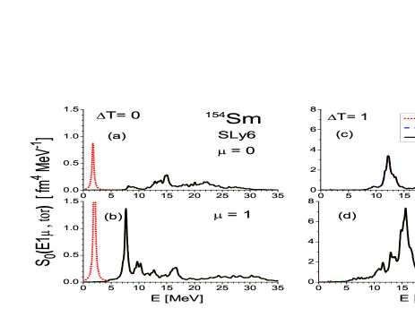
Figure 3: The same as in the Fig.2 but for toroidal $E1$ response.

In Fig. 3, the SA-elimination effect for the toroidal $E1$ excitations is illustrated. Unlike CM$(\Delta T=0)$ case in Fig. 2, SA in TM($\Delta T=0$) strength is almost fully concentrated in the lowest peak while the strength at a higher energy is not contaminated. The difference in SA-pollution for CM and TM is explained by different character of these modes. CM is irrotational and so is strongly affected by CoM which is also irrotational. Instead TM is basically vortical Kv11 and so the CoM impact on TM is much less. For TM($\Delta T=1$), the pollution is almost absent. Fig. 3 shows that our procedure fully suppresses spurious peaks in TM$(\Delta T=0)$. In all the plots, the green dashed and black solid lines are practically coincide, i.e. effect of the deformation-induced corrections $d^{\mu}_{0,1}$ is negligible. This is explained by a small (as compared to CM) relative weight of $d^{\mu}_{0,1}$ in the toroidal SA-corrections given in (67)-(68).

IV.2 Elimination of SA from $E0$ and $E20$ excitations

The pairing treated within Bardeen–Cooper–Schrieffer (BCS) procedure leads to violation of the conservation law (21) for the particle number $N_{q}$ Ri80 . This results in spurious admixtures in electric monopole $E0$ and quadrupole $E20$ excitations with $K=0$. Time-even operators for E0 and E20 transitions are

$$\hat{\mathcal{M}}_{E\lambda 0}^{(\Delta T)}=\sum_{q=n,p}e^{(\Delta T)}_{q}\sum_{k\in q}(r^{2}Y_{\lambda 0})_{k}$$ (69)

with $\lambda$=0 and 2.

The symmetry operator is the time-even operator of the particle number $\hat{N}_{q}$. It can be associated with the spurious operator $\hat{X}_{0}$ (for simplicity of notation, we omit below the index $q$). Then, within BCS, we get

$$\hat{X}_{0}=\hat{N}=\sum_{j>0}\mathcal{X}^{(0)}_{j{\bar{j}}}\big{(}\alpha^{+}_{j}\alpha^{+}_{\bar{j}}+\alpha_{\bar{j}}\,\alpha_{j}\big{)}$$ (70)

with $\mathcal{X}^{(0)}_{j\bar{j}}=2\>\mathcal{U}_{j}\mathcal{V}_{j}$ and $\mathcal{U}_{j}$, $\mathcal{V}_{j}$ being BCS pairing amplitudes. Following (10b) the time-odd conjugate spurious operator is

$$\hat{\mathcal{P}}_{0}=\sum_{ij}\mathcal{P}^{(0)}_{ij}\,\big{(}\alpha^{+}_{i}\alpha^{+}_{j}-\alpha_{\bar{j}}\alpha_{\bar{i}}\big{)}\,.$$ (71)

Since the values $\mathcal{X}^{(0)}_{j{\bar{j}}}$ are known, we can obtain their conjugates $\mathcal{P}^{(0)}_{ij}$ from (39). Then, using (91) from Appendix B, we can calculate the averages $\langle 0|\,\big{[}Q_{\nu},\,\hat{\mathcal{M}}\big{]}\,|0\rangle$, determine the coefficients $\alpha_{\nu}$ and $\beta_{\nu}$, and finally build refined states. Just this prescription was used to get the numerical results shown in this subsection. It partly reminds the earlier projection scheme proposed for E0 excitations in Ju08 . However, our prescription is more general. As shown below, we also suggest the direct refinement of the transition matrix elements and operators.

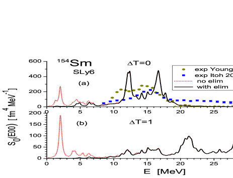
Figure 4: Skyrme QRPA strength function (41) for isoscalar (top panel) and isovector (bottom panel) $E0$ transitions. Results for $\Delta T$=0 are compared with $(\alpha,\alpha^{\prime})$ experimental data of D.H. Youngblood et al Yo04 and M. Itoh et al It03 . The strengths without (red dotted curve) and with (black solid curves) SA-elimination are shown.

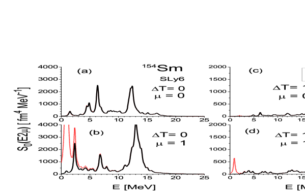
Figure 5: Isoscalar (left) and isovector (right) $E20$ ($\mu$=0) and $E21$ ($\mu$=1) strength functions calculated without (red dotted curves) and with (black solid curves) SA-elimination.

As an alternative way, we can also construct the refined transition operator. Following (34), it reads

$$\hat{\tilde{\mathcal{M}}}^{(\Delta T)}_{E\lambda 0} = \hat{\mathcal{M}}^{(\Delta T)}_{E\lambda 0}-\frac{i}{\hbar}\langle 0|[\hat{P}^{\dagger}_{0},\hat{\mathcal{M}}^{(\Delta T)}_{E\lambda 0}]|0\rangle\hat{N}$$

$$= \hat{\mathcal{M}}^{(\Delta T)}_{E\lambda 0}-\gamma^{(\Delta T)}_{E\lambda 0}\hat{N}.$$

with

$$\gamma^{(\Delta T)}_{E\lambda 0} = \frac{i}{\hbar}\langle 0|[\hat{P}^{\dagger}_{0},\hat{\mathcal{M}}^{(\Delta T)}_{E\lambda 0}]|0\rangle$$

$$= \frac{2i}{\hbar}\sum_{ij}[\mathcal{P}^{(0)}_{ij}]^{*}\langle ij|\hat{\mathcal{M}}^{(\Delta T)}_{E\lambda 0}|0\rangle.$$

In quasiparticle representation,

$$\hat{\tilde{\mathcal{M}}}^{(\Delta T)}_{E\lambda 0}=\sum_{ij}\langle ij|\hat{\tilde{\mathcal{M}}}^{(\Delta T)}_{E\lambda 0}|0\rangle\big{(}\alpha^{+}_{i}\alpha^{+}_{j}+\alpha_{\bar{j}}\,\alpha_{\bar{i}}\big{)}$$ (74)

with

$$\langle ij|\hat{\tilde{\mathcal{M}}}^{(\Delta T)}_{E\lambda 0}|0\rangle=\langle ij|\hat{\mathcal{M}}^{(\Delta T)}_{E\lambda 0}|0\rangle-2\gamma^{(\Delta T)}_{E\lambda 0}\delta_{\bar{i}j}\mathcal{U}_{j}\mathcal{V}_{j}.$$ (75)

So, to exclude SA, the transition operator can be corrected only in matrix elements with $|j\bar{j}\rangle$. The factor $\mathcal{U}_{j}\mathcal{V}_{j}$ is large only for states near the Fermi level and, therefore, just these states mainly contribute to the correction.

The SA-elimination effect for the monopole strength $S_{0}(E0)$ and quadrupole strength $S_{0}(E20)$ is demonstrated in Figs. 4 and 5. Both strengths embrace the same set of QRPA $K^{\pi}=0^{+}$ states calculated with the particle-particle channel Rep17EPJA .

Fig. 4 illustrates elimination of SA from the isoscalar and isovector $E0$ responses calculated with effective charges from (51). In the upper panel, the calculated strength $S_{0}(E0)$ rather well reproduces experimental data Yo04 . Both features, two-hump structure of the Giant Monopole Resonance (GMR) and vanishing the strength above GMR, are described. At the same time, $S_{0}(E0)$ deviates in these features from the data It03 . There is a definite discrepancy between the data Yo04 and It03 , though both of them are obtained from $(\alpha,\alpha^{\prime})$ reaction, see discussion in Kv16E0 .

Figure 4 shows that in both $\Delta T=0$ and $\Delta T=1$ channels SA are not merely concentrated in the lowest peak but essentially contaminate low-energy excitations at $E<$8 MeV. At the higher energy, the pollution is negligible. Our procedure successfully removes the spurious strength.

In the top panels of Fig. 5, the quadrupole strength $S_{0}(E20)$ with and without SA-elimination is demonstrated. In contrast to E0 case, the SA contamination is almost negligible. Some elimination effect is visible only for the minor lowest spurious peak at $E\approx$ 2 MeV in $\Delta T$=1 channel. The difference in the pollution of $E0$ and $E2$ strengths can be explained by basically monopole character of the pairing. So just $E0$ but not $E2$ strength is contaminated.

IV.3 Elimination of SA from $E21$ and $M11$ excitations

The rotational invariance is related with the conservation of the total angular momentum $\hat{\bf J}$ of the nucleus Mar69 ; Row70 ; Ri80 . Since in axial deformed nuclei the rotation around the intrinsic symmetry z-axis is forbidden, the conservation law is formulated through $\mu=\pm 1$ components of $\hat{\bf J}$, combining intrinsic x- and y-axes:

$$\big{[}\,\hat{H}_{\rm{intr}},\hat{J}_{\mu=\pm 1}\,\big{]}=0.$$ (76)

Below we consider only

$$\hat{J}_{1}=-\frac{1}{\sqrt{2}}(\hat{J}_{x}+i\hat{J}_{y})=\hat{L}_{1}+\frac{1}{2}\sigma_{1}$$ (77)

where $\hat{L}_{1}$ and $\sigma_{1}$ are components of the angular momentum and Pauli matrix for $\mu$=1. The violation of the conservation law (76) leads to SA in $K^{\pi}=1^{+}$ states and contaminates $E21$ and $M11$ transitions between these states and the ground state. The symmetry operator $\hat{J}_{1}$ is time-odd and so can be associated with the spurious operator $\hat{\mathcal{P}}_{0}$ Mar69 ; Ri80 ; KvNa86 :

$$\hat{J}_{1}=\hat{\mathcal{P}}_{0}=\sum_{ij}\mathcal{P}^{(0)}_{ij}\,\big{(}\alpha^{+}_{i}\alpha^{+}_{j}-\alpha_{\bar{j}}\alpha_{\bar{i}}\big{)}$$ (78)

where $\mathcal{P}^{(0)}_{ij}=\langle ij|\,\hat{J}_{1}\,|0\rangle$ are real two-quasiparticle matrix elements. The angle operator $\hat{\Theta}$, being the time-even conjugate to $\hat{J}_{1}$, matches the spurious operator $\hat{\mathcal{X}}_{0}$ Ri80 :

$$\hat{\Theta}_{1}\equiv\hat{\mathcal{X}}_{0}=\sum_{ij}\mathcal{X}^{(0)}_{ij}\,\big{(}\alpha^{+}_{i}\alpha^{+}_{j}+\alpha_{\bar{j}}\alpha_{\bar{i}}\big{)}$$ (79)

where $\langle ij|\,\hat{\mathcal{X}}_{0}\,|0\rangle$ are imaginary. The operators obey the normalization condition $\big{[}\,\hat{\mathcal{X}}_{0},\,\hat{\mathcal{P}}_{0}^{\dagger}\,\big{]}=\big{[}\,\hat{\Theta}_{1},\,\hat{J}_{1}^{\dagger}\,\big{]}=i\hbar$. Using known matrix elements $\mathcal{P}^{(0)}_{ij}=J^{(1)}_{ij}=\langle ij|\,\hat{J}_{1}\,|0\rangle$, the values $\mathcal{X}^{(0)}_{ij}$ are obtained from the inversion equation (37). Then, as in the previous subsection, we can calculate the averages $\langle 0|\,\big{[}Q_{\nu},\,\hat{\mathcal{M}}\big{]}\,|0\rangle$, determine the coefficients $\alpha_{\nu}$ and $\beta_{\nu}$, and finally construct the refined QRPA states. This way was utilized to get the numerical results shown below.

The parameter $M_{0}$ is calculated combining (38) with (22). It has the physical meaning of the principal $\mu=1$ component of the moment of inertia $\mathcal{F}_{1}$ Mar69 ; Ri80 ; KvNa86 :

$$M_{0}=\mathcal{F}_{1}\approx 2\sum_{ij,kl}\!J^{(1)\,*}_{ij}\,(A-B)^{-1}_{ij,\,kl}\,J^{(1)}_{kl}\;.$$ (80)

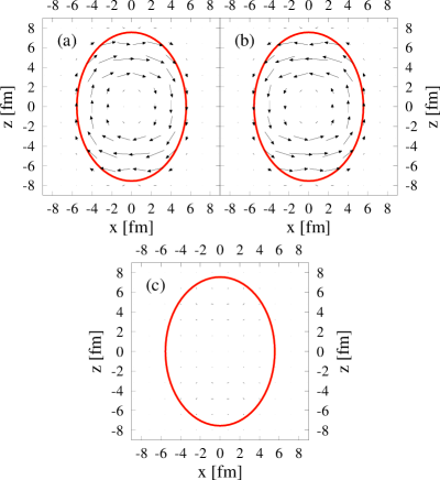
Figure 6: The convective isoscalar current transition density in the x-z plane of the intrinsic frame, calculated following (33) for the first ($\nu=0$) spurious QRPA $K^{\pi}=1^{+}$ solution with the energy $\hbar\omega_{0}=\>0.95$ MeV. The panels show: (a) $\delta{\bf j}_{\nu=0}^{(\Delta T=0)}({\bf r})$ without SA-elimination, (b) the SA-correction term in the r.h.s of (33), (c) $\delta{\bf j}_{\nu^{\prime}=0}^{(\Delta T=0)}({\bf r})$ with SA-elimination.

The $E21$ and $M11$ transition operators are characterized by the time-even operator

$$\hat{\mathcal{M}}_{E21}^{(\Delta T)}=\sum_{q=n,p}e^{(\Delta T)}_{q}\sum_{k\in q}(r^{2}Y_{21})_{k}$$ (81)

and the time-odd operator

$$\hat{\mathcal{M}}_{M11}^{(\Delta T)}=\frac{e\hbar}{2mc}\sqrt{\frac{3}{4\pi}}\,\sum_{q=n,p}\sum_{k\in q}\big{[}e^{(\Delta T)}_{q}\,\hat{l}^{(k)}_{1}+g_{q}\,\hat{s}^{(k)}_{1}\big{]}$$ (82)

where $\hat{l}^{(k)}_{1}$ and $\hat{s}^{(k)}_{1}$ are ($\mu$=1)-components of operators of the orbital momentum and spin for $k$-th nucleon. Further, $e^{(\Delta T)}_{q}$ are effective charges. They are taken as (51) for $E21$ and as $e^{(\Delta T)}_{p}$=1 and $e^{(\Delta T)}_{n}$=0 for $M21$. Gyromagnetic factors $g_{q}=g^{s}_{q}\eta$ are composed from the nucleon bare factors $g^{s}_{q}$ with the quenching parameter $\eta$=0.7 Ha01 .

The corresponding refined operators are

$$\hat{\tilde{\mathcal{M}}}^{(\Delta T)}_{E21} = \hat{\mathcal{M}}^{(\Delta T)}_{E21}-\frac{i}{\hbar}\langle 0|[\hat{J}_{1}^{\dagger},\hat{\mathcal{M}}^{(\Delta T)}_{E21}]|0\rangle\hat{\Theta}_{1}\;,$$ (83)

$$\hat{\tilde{\mathcal{M}}}^{(\Delta T)}_{M11} = \hat{\mathcal{M}}^{(\Delta T)}_{M11}+\frac{i}{\hbar}\langle 0|[\hat{\Theta}_{1}^{\dagger},\hat{\mathcal{M}}^{(\Delta T)}_{M11}]|0\rangle\hat{J}_{1}\;.$$ (84)

Following Appendix B, the average commutators in (83) and (84) can be computed as

$$\langle 0|[\hat{J}_{1}^{\dagger},\hat{\mathcal{M}}^{(\Delta T)}_{E21}]|0\rangle = 2\,\sum_{ij}[\mathcal{P}_{ij}^{(0)}]^{*}\,\langle ij|\,\hat{\mathcal{M}}^{(\Delta T)}_{E21}\,|0\rangle,$$ (85)

$$\langle 0|[\hat{\Theta}_{1}^{\dagger},\hat{\mathcal{M}}^{(\Delta T)}_{M11}]|0\rangle = 2\,\sum_{ij}[\mathcal{X}_{ij}^{(0)}]^{*}\,\langle ij|\,\hat{\mathcal{M}}^{(\Delta T)}_{M11}\,|0\rangle.$$ (86)

SA-corrections in (83) and (84) include $\hat{J}_{1}$ and, in this sense, correspond to the corrections suggested earlier in Mar69 ; Ri80 ; KvNa86 .

In the bottom ($\mu=1$) plots of Fig. 5, we demonstrate subtraction of SA from $E21$ responses. The plots show the strong elimination effect for low-energy states, especially in $\Delta T=0$ channel.

To illustrate the elimination mechanism, we show in Fig. 6 the convective part of the isoscalar current transition density (33) for the spurious $K^{\pi}=1^{+}$ state at 0.95 MeV (this state is depicted by the dotted red line in $\Delta T=0$ and $\Delta T=1$ bottom plots of Fig. 5). Following (33), the refined current transition density $\delta\bf{j}_{\nu^{\prime}=0}$ is the sum of the initially polluted $\delta\bf{j}_{\nu=0}$ and the correction current. In the plot (a) with $\delta\bf{j}_{\nu=0}$, we see a clear spurious rotation. The SA-correction current shown in the plot (b) demonstrates the opposite rotation. These two currents compensate each other and thus give the vanishing $\delta\bf{j}_{\nu^{\prime}=0}$ in the plot (c).

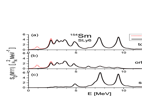
Figure 7: The total (top), orbital (middle) and spin (bottom) $M11$ strength functions calculated without (red dotted line) and with (black solid line) SA-elimination.

Further, Fig. 7 shows the SA-elimination effect for $M1(K=1)$ strength in ¹⁵⁴Sm. The strength functions are calculated for $M11$ transition operator (82) consisting of the orbital and spin parts. As seen from the figure, orbital part of $M11$-operator generates $M1(K=1)$ orbital scissor mode located at 2-4 MeV (plot (b)) while spin part of the operator produces the spin-flip resonance lying at 6-11 MeV (plot (c)). We see that the spuriosity caused by the nuclear rotation concerns only the low-energy orbital part of $M11$ strength. Our SA-elimination method fully suppresses the spurious peak at 0.95 MeV in the orbital $M11$ strength.

IV.4 Comparison with other approaches

In our method, we get the refined QRPA physical states from the condition (23)-(24), i.e. requesting orthogonality of physical states to the spurious mode (which can be also considered as projection of contaminated states onto refined physical states). This simple and evident condition was also used in some previous works, e.g. Co00 ; Ju08 ; Ars10 ; Na07 ; Mi12 . Let’ briefly compare our and previous studies.

The works Co00 ; Ju08 ; Ars10 consider subtraction of SA from compression $E1(\Delta T=0)$ Co00 , monopole $E0(\Delta T=0)$ Ju08 , and dipole $E1(\Delta T=1)$Ars10 QRPA states in spherical nuclei. The principle difference of our approach with these works is that we use a more general expression (20) for the spurious state where both $\hat{\mathcal{X}}_{0}$ and $\hat{\mathcal{P}}_{0}$ operators are included. This allows us to get, in the same theoretical frame, the general SA-subtraction recipe covering various symmetry violations.

In works Na07 ; Mi12 , the spurious state embraces both time-even and time-odd parts. However these works deal with specific QRPA versions: finite amplitude method Na07 and Green’s function method Mi12 . So their recipes have specific forms determined by particular QRPA realizations. Besides these recipes address only transition densities Na07 or strength functions Mi12 . Instead, our method is based on the conventional matrix QRPA and suggests SA-elimination for a wider set of characteristics: wave functions, transition matrix elements (transition densities), and transition operators.

Altogether, the major differences and advantages of our method as compared to the previous studies Co00 ; Ju08 ; Na07 ; Mi12 ; Ars10 , can be summarized as:

a) Unlike Co00 ; Ju08 ; Ars10 ; Na07 ; Mi12 , we propose SA-corrections at different stages of the calculations: for QRPA states, matrix elements and even transition operators. Various symmetry violations can be covered, both spherical and deformed nuclei can be considered. This flexibility is indeed important in practical calculations.

b) Our method reproduces well known SA-corrections for conventional $E1(\Delta T=1)$ Ri80 , compression $E1(\Delta T=0)$ VG81 ; Kv11 and toroidal $E1(\Delta T=0)$ Vre02tor ; Kv11 excitations, obtained earlier in different models. In Co00 ; Ju08 ; Ars10 ; Na07 ; Mi12 , these corrections are considered as independent items to be compared with the projection results. We show that the previous corrections can be derived on the same theoretical footing within the projection technique. This deepens our knowledge on the nature and accuracy of SA-elimination in dipole states.

c) For the first time, deformation-induced analytical corrections for $E1$ compression and toroidal transitions were derived and numerically tested. They were found to be essential for compression $E1(\Delta T=0)$ low-energy excitations.

V Conclusion

A general simple method for elimination of spurious admixtures (SA) from RPA/QRPA intrinsic nuclear excitations is proposed. The SA-corrections are derived from the requirement of orthogonality of physical QRPA states to the phonon-like spurious state. Within this projection technique, the most relevant cases are inspected: violation of the translational invariance (ordinary, compression and toroidal $E1$ modes), pairing-induced non-conservation of the particle number ($E2(K=0)$ and $E0$ modes), and violation of the rotational invariance ($E2(K=1$) and $M1(K=1)$ modes). Various familiar SA-corrections are rederived on the same theoretical footing and new elimination schemes are proposed.

For each relevant case, the SA-subtraction is illustrated by Skyrme QRPA calculations for axially deformed ¹⁵⁴Sm. High efficiency and accuracy of the method are demonstrated.

The method is universal. Both isoscalar ($\Delta T$ = 0) and isovector ($\Delta T$ = 1) excitations are covered. The refinement from SA can be carried out at different levels of calculations: for each RPA/QRPA state and directly for various electric and magnetic responses. In the later case, the SA-corrections are derived for transition matrix elements and even for transition operators. For $E1$ excitations, the analytical expressions for SA-corrections are proposed. For axial deformed nuclei, the additional deformation-induced SA-corrections for the compression and toroidal $E1$ strengths are derived. It is shown that these corrections are important for the low-energy part of the $E1(\Delta T$ = 0) compression mode. The method can be applied to various RPA/QRPA approaches including self-consistent ones.

Appendix A Operators of nuclear density and current

The density operator is

$$\hat{\rho}^{(\Delta T)}({\bf r})=e\sum_{q=n,p}e^{(\Delta T)}_{q}\sum_{k\in q}\delta({\bf r}-{\bf r}_{k})$$ (87)

with the effective charges $e^{(0)}_{p}=e^{(0)}_{n}=1$ in the isoscalar ($\Delta T$=0) case and $e^{(1)}_{p}=-e^{(1)}_{n}=1$ in the isovector ($\Delta T$=1) case.

The operator of the nuclear current

$$\hat{\bf j}^{(\Delta T)}({\bf r})=\hat{\bf j}_{\rm c}^{(\Delta T)}({\bf r})+\hat{\bf j}_{\rm m}^{(\Delta T)}({\bf r})$$ (88)

consists from the convective and magnetization parts

$$\hat{\bf j}_{\rm c}^{(\Delta T)}({\bf r}) = -i\frac{e\hbar}{2m}\sum_{q=n,p}e^{(\Delta T)}_{q}$$

$$\cdot \sum_{k\in q}\big{[}\delta({\bf r}-{\bf r}_{k})\,{\bf\nabla}_{k}+{\bf\nabla}_{k}\,\delta({\bf r}-{\bf r}_{k})\big{]},$$

$$\hat{{\bf j}}_{\rm m}^{(\Delta T)}({\bf r}) = \frac{e\hbar}{2m}\sum_{q=n,p}g_{q}\sum_{k\in q}{\bf\nabla}\times\hat{{\bf s}}_{k}\;\delta({\bf r}-{\bf r}_{k}).$$ (90)

Here $m$ is the nucleon mass, $\hat{s}$ is the spin operator, $g_{q}$ is the nucleon gyromagnetic factor.

Appendix B Commutator averages

If $\hat{\mathcal{M}}=\sum_{ij}\langle ij|\hat{\mathcal{M}}|{\rm BCS}\rangle(\alpha^{+}_{i}\alpha^{+}_{j}+\gamma_{\mathcal{T}}^{\mathcal{M}}\alpha_{\bar{j}}\alpha_{\bar{i}})$, then averages in (30) - (35) have the form:

$$\langle 0|\,\big{[}Q_{\nu},\,\hat{\mathcal{M}}\big{]}\,|0\rangle=$$ (91)

$$\quad=\sum_{ij}\big{[}X^{(\nu)*}_{ij}+\gamma_{\mathcal{T}}^{\mathcal{M}}Y^{(\nu)*}_{ij}\big{]}\,\langle ij|\,\hat{\mathcal{M}}\,|{\rm BCS}\rangle\>,$$

$$\langle 0|\,\big{[}\hat{\mathcal{X}}_{0}^{\dagger},\,\hat{\mathcal{M}}\big{]}\,|0\rangle=$$ (92)

$$\ =\begin{cases}0\qquad\qquad\qquad\qquad\qquad\quad\text{ for time-even }\hat{\mathcal{M}}\\[2.0pt] \begin{array}[]{l}2\,\sum_{ij}\mathcal{X}_{ij}^{(0)\,*}\,\langle ij|\,\hat{\mathcal{M}}\,|{\rm BCS}\rangle\>\text{ for time-odd }\hat{\mathcal{M}}\;,\end{array}\end{cases}$$

$$\langle 0|\,\big{[}\hat{\mathcal{P}}_{0}^{\dagger},\,\hat{\mathcal{M}}\big{]}\,|0\rangle=$$ (93)

$$\ =\begin{cases}\begin{array}[]{l}2\,\sum_{ij}\mathcal{P}_{ij}^{(0)\,*}\,\langle ij|\,\hat{\mathcal{M}}\,|{\rm BCS}\rangle\>\text{ for time-even }\hat{\mathcal{M}}\end{array}\\[2.0pt] 0\qquad\qquad\qquad\qquad\qquad\quad\text{ for time-odd }\hat{\mathcal{M}}\;,\end{cases}$$

where $|{\rm BCS}\rangle$ is the BCS vacuum.

Appendix C Skyrme QRPA framework

The total functional ${\mathcal{E}}_{\rm tot}$ includes Skyrme, Coulomb and pairing parts Re92 ; Be03 ; Rep17EPJA :

$${\mathcal{E}}_{\rm tot}={\mathcal{E}}_{\rm Sk}+{\mathcal{E}}_{\rm Coul}+{\mathcal{E}}_{\rm pair}\;.$$ (94)

The Skyrme part ${\mathcal{E}}_{\rm Sk}\{J^{\varsigma}_{q}\}$ depends on the set $\{J^{\varsigma}_{q}\}$ of densities and currents (listed by $\varsigma$) for protons and neutrons ($q$=p,n). This set includes time-even (nucleon $\rho_{q}$, kinetic-energy $\tau_{q}$, spin-orbit ${\bf J}_{q}$) and time-odd (current ${\bf j}_{q}$, spin ${\bf s}_{q}$, vector kinetic-energy ${\bf T}_{q}$) items. The Coulomb functional ${\mathcal{E}}_{\rm Coul}(\rho_{p})$ consists from the direct term and exchange terms in Slater approximation Be03 ; Rep17EPJA .

The pairing functional ${\mathcal{E}}_{\rm pair}(\rho_{q})$ can be taken in the surface and volume forms, i.e. with and without the density dependence Be00 ; Rep17EPJA . For simplicity reasons, we consider here the volume form

$$\mathcal{E}_{\rm pair}=\frac{1}{4}\>\sum_{q=n,p}V_{q}\>\int d^{3}r\>|\tilde{\rho}_{q}({\bf r})|^{2}$$ (95)

where $V_{q}$ are neutron and proton pairing constants and

$$\tilde{\rho}_{q}({\bf r})=2\sum_{i\epsilon q}f_{i}^{q}v_{i}u_{i}|\psi_{i}({\bf r})|^{2}$$ (96)

are pairing densities with single-particle wave functions $\psi_{i}({\bf r})$, Bogoliubov pairing factors $v_{i}$ and $u_{i}$ and energy-dependent cut-off weights $f^{q}_{i}$ Rep17EPJA .

The nuclear mean field is determined by Hartree-Fock method using first functional derivatives $\delta({\mathcal{E}}_{\rm Sk}+{\mathcal{E}}_{\rm Coul})/\delta J^{\varsigma}_{q}$ over time-even densities $J^{\varsigma}_{q}$. The volume pairing is treated within the BCS scheme Rep17EPJA .

The residual interaction is determined by the second functional derivatives $\delta^{2}{\mathcal{E}}_{\rm tot}/\delta J^{\varsigma}_{q}\delta J^{\varsigma^{\prime}}_{q^{\prime}}$ Rep17EPJA . The contributions of all time-even and time-odd densities and currents, including the pairing density (96), is taken into account. Both particle-hole (ph) and pairing-induced particle-particle (pp) channels are involved, see detailed expressions in Rep17EPJA . In ph-channel, Coulomb contribution is included.

Our QRPA approach is fully self-consistent since i) both the mean field and residual interaction are obtained from the same initial functional, ii) contributions of all the densities and currents are taken into account, iii) both ph- and pp-channels are considered.

Appendix D Useful relations

In derivation of SA corrections to E1 transition operators, the following relations were used Va76 :

$$\nabla_{0}r^{3}Y_{10}(\hat{r}) =\frac{1}{\sqrt{3}}\,\Big{[}5r^{2}Y_{00}+\frac{4}{\sqrt{5}}r^{2}Y_{20}(\hat{r})\Big{]},$$ (97)

$$\nabla_{\pm 1}r^{3}Y_{1,\mp 1}(\hat{r}) =\frac{1}{\sqrt{3}}\,\Big{[}{-}5r^{2}Y_{00}+\frac{2}{\sqrt{5}}r^{2}Y_{20}(\hat{r})\Big{]},$$ (98)

$$Y_{00}=1/(2\sqrt{\pi}),$$ (99)

$$[{\bf Y}^{0}_{1\mu}]^{*}\cdot{\bf Y}^{2}_{1\mu} = \frac{1}{\sqrt{40\pi}}Y_{20}\,c_{\mu},$$ (100)

$$[{\bf Y}^{0}_{1\mu}]^{*}\cdot{\bf Y}^{0}_{1\mu} = \frac{1}{4\pi}$$ (101)

where $c_{\mu}$=-2 for $\mu$=0 and 1 for $\mu=\pm 1$.

References

- (1) D.J. Thouless, Nucl. Phys. 22, 78 (1961).
- (2) D.J. Thouless nd J.G. Valatin, Nucl. Phys. 31, 211 (1962).
- (3) E.R. Marshalek and J. Weneser, Ann. Phys. (NY) 53, 569 (1969).
- (4) D.J. Rowe, Nuclear Collective Motion (Mothuen, London, 1970).
- (5) P. Ring and P. Schuck, Nuclear Many Body Problem (Springer-Verlag N.Y.-Hedelberg-Berlin, 1980).
- (6) J.P. Blaizot and G. Ripka, Quantum Theory of Finite Systems, Ch. 10 (MIT Press, Cambridge, MA, 1986).
- (7) N. Van Giai and H. Sagawa, Nucl. Phys. A 371, 1 (1981).
- (8) M.N. Harakeh, and A. van der Woude, Giant Resonances (Clarendon Press Oxford, 2001).
- (9) E.B. Balbutsev, I.V. Molodtsova, and A.V. Unzhakova, Europhys. Lett. 26, 499 (1994).
- (10) J. Kvasil, V.O. Nesterenko, W. Kleinig, P.G. Reinhard, and P. Vesely, Phys. Rev. C 84, 034303 (2011).
- (11) P.-G. Reinhard, Ann. Phys. (Leipzig) 504, 632 (1992).
- (12) M. Bender, P.-H. Heenen, and P.-G. Reinhard, Rev. Mod. Phys. 75, 121 (2003).
- (13) T. Nikšić, D. Vretenar, and P. Ring, Phys. Rev. C 74, 064309 (2006).
- (14) L.M. Robledo, T.R. Rodríguez, R.R. Rodíguez-Guzmán, arXiv:1807.02518v1[nucl-th].
- (15) G. Colo, N. Van Giai, P.F. Bortignon, and M.R.Qualia, Phys. Lett. B485, 362 (2000).
- (16) Jun Li, G. Colo, and J. Meng, Phys. Rev. C 78, 064304 (2008).
- (17) N.N. Arsenyev abnd A.P. Severyukhin, Phys. Part. Nucl. Lett. 7, 112 (2010).
- (18) T. Nakatsukasa, T. Inakura, and K. Yabana, Phys. Rev. C 76, 024318 (2007).
- (19) K. Mizuyama and Gianluca Colo, Phys. Rev. C 85, 024307 (2012).
- (20) D. Vretenar, N. Paar, and P. Ring, Phys. Lett. B 487, 334 (2000).
- (21) D. Vretenar, N. Paar, P. Ring, and T. Nikšić, Phys. Rev. C 65, 021301(R) (2002).
- (22) N. Paar, D. Vretenar, E. Khan, and G. Colo, Rep. Prog. Phys. 70, 691 (2007).
- (23) W. Kleinig, V.O. Nesterenko, J. Kvasil, P.-G. Reinhard and P. Vesely, Phys. Rev. C 78, 044313 (2008).
- (24) J. Kvasil, V.O. Nesterenko, A. Repko, W. Kleinig, and P.-G. Reinhard, Phys. Rev. C 94, 064302 (2016).
- (25) J. Terasaki and J. Engel, Phys. Rev. C 82, 034326 (2010).
- (26) V.O. Nesterenko, V.G. Kartavenko, W. Kleinig, J. Kvasil, A. Repko, R.V. Jolos, and P.-G. Reinhard, Phys. Rev. C 93, 034301 (2016).
- (27) J. Kvasil and R.G. Nazmitdinov, Sov. J. Part. Nucl. 17, 265 (1986).
- (28) H. Nakada, Prog. Theor. Exp. Phys. 023D02, 099101 (2016).
- (29) N.I. Pyatov and D.I. Salamov, Nucleonika 22, 127 (1977).
- (30) F. Palumbo, Nuclear Physics 99, 100 (1967)
- (31) F. Donau, Phys. Rev. Lett. 94, 092503 (2005).
- (32) V.O. Nesterenko, J. Kvasil, and P.-G. Reinhard, Phys. Rev. C 66, 044307 (2002).
- (33) V.O. Nesterenko, W. Kleinig, J. Kvasil, P. Vesely, P.- G. Reinhard, and D. S. Dolci, Phys. Rev. C 74, 064306 (2006).
- (34) Ll. Serra, R.G. Nazmitdinov, and A. Puente, Phys. Rev. B 68, 035341 (2003).
- (35) A. Repko, J. Kvasil, V.O. Nesterenko, and P.-G. Reinhard, Eur. Phys. J. A 53, 221 (2017).
- (36) A. Repko, Theoretical description of nuclear collective excitations, PhD thesis, Math.-Phys. Faculty of Charles University in Prague (2015), arXiv:1603.04383 [nucl-th].
- (37) A. Repko, J. Kvasil, V.O. Nesterenko, and P.-G. Reinhard, arXiv:1510.01248v3 [nucl-th].
- (38) E. Chabanat, P. Bonche, P. Haensel, J. Meyer, R. Schaeffer, Nucl. Phys. A635, 231 (1998).
- (39) J. Kvasil, V.O. Nesterenko, W. Kleinig, D. Bozik, P.-G. Reinhard, N. Lo Iudice, Eur. Phys. J. A49, 119 (2013).
- (40) V.O. Nesterenko, A. Repko, J. Kvasil, and P.-G. Reinhard, Phys. Rev. Lett. 120, 182501 (2018).
- (41) V.O. Nesterenko, J. Kvasil, A. Repko, and P.-G. Reinhard, Eur. Phys. J. Web of Conf. 194, 03005 (2018).
- (42) D. A. Varshalovich, A. N. Moskalev, and V. K. Khersonskii, Quantum Theory of Angular Momentum (World Scientific, Singapore, 1976).
- (43) G.M. Gurevich, L.E. Lazareva, V.M. Mazur, S.Yu Merkulov, G.V. Solodukov, and V.A. Tyutin, Nucl. Phys. A351, 257 (1981).
- (44) D.H. Youngblood, Y.W. Lui, H.L. Clark, B. John, Y. Tokimoto, and X. Chen, Phys. Rev. C69, 034315 (2004).
- (45) M. Itoh, H. Sakaguchi,M. Uchida, T. Ishikawa, T. Kawabata, T. Murakami, H. Takeda, T. Taki, S. Terashima, N. Tsukahara, Y. Yasuda, M. Yosoi, U. Garg, M. Hedden, B. Kharraja, M. Koss, B. K. Nayak, S. Zhu, H. Fujimura, M. Fujiwara, K. Hara, H. P. Yoshida, H. Akimune, M. N. Harakeh, and M. Volkerts, Phys. Rev. C68, 064602 (2003).
- (46) A. Bohr and B. R. Mottelson, Nuclear Structure (Benjamin, New York, 1969), Vol. 1.
- (47) M. Bender, K. Rutz, P.-G. Reinhard, J.A. Maruhn, Eur. Phys. J. A 8, 59 (2000).