A “poor man’s” approach to topology optimization of natural convection problems

Abstract

Topology optimization of natural convection problems is computationally expensive, due to the large number of degrees of freedom (DOFs) in the model and its two-way coupled nature. Herein, a method is presented to reduce the computational effort by use of a reduced-order model governed by simplified physics. The proposed method models the fluid flow using a potential flow model, which introduces an additional fluid property. This material property currently requires tuning of the model by comparison to numerical Navier-Stokes based solutions. Topology optimization based on the reduced-order model is shown to provide qualitatively similar designs, as those obtained using a full Navier-Stokes based model. The number of DOFs is reduced by 50% in two dimensions and the computational complexity is evaluated to be approximately 12.5% of the full model. We further compare to optimized designs obtained utilizing Newton’s convection law.

topology optimization, natural convection, reduced-order model, potential flow, heat sink design

1 Introduction

Natural convection is the study of temperature-driven flow. Differences in spatial temperature cause density gradients in the fluid, which in turn cause fluid motion due to buoyancy. This then induces transport of energy in the form of convection. Natural convection is thus a strongly two-way coupled problem, in which the temperature field has great impact on the velocity field and vice versa.

In this paper, a reduced-order model is presented based on potential flow. The model can be shown to be equivalent to Darcy’s law for flow in porous media, with a fictitious permeability in the fluid domain. This flow model is coupled to the heat transport, which is modeled by a convection-diffusion equation, through the use of the Boussinesq approximation. In comparison to modeling the full Navier-Stokes equations, the reduction in system dimension is significant, as the velocities can be computed explicitly from the pressure and temperature fields, allowing for omission of all velocity degrees-of-freedom (DOFs) from the system solve and computing them as a post-processing step.

The huge savings in CPU time come at the expense of reduced accuracy of the physical modeling. However, as will be demonstrated, optimized designs are remarkably similar to those obtained with the full Navier-Stokes model.

Topology optimization originates from solid mechanics (Bendsøe and Kikuchi, 1988; Bendsøe and Sigmund, 2003), but has been extended to many other physics (Deaton and Grandhi, 2014) in the recent decades. Curiously, topology optimization was applied to thermomechanical structures (Rodrigues and Fernandes, 1995; Sigmund, 2001; Yin and Ananthasuresh, 2002) before pure heat conduction problems (Bendsøe and Sigmund, 2003; Donoso and Sigmund, 2004; Gersborg-Hansen et al, 2006). Recently, pure heat conduction problems were revisited and it was revolutionarily shown that optimal structures for the famous volume-to-point problem are lamelar needle-like structures (Yan et al, 2018), and not the commonly observed tree-like branching structures. Shifting perspective to fluid flow problems, topology optimization was first applied to Stokes flow by Borrvall and Petersson (2003) using a resistance term based on the out-of-plane channel flow thickness. This approach was later extended to Navier-Stokes flow by (Gersborg-Hansen et al, 2005). Over time, the approach has shifted to the use of a Brinkman penalization term to model an immersed solid geometry embedded in a fluid domain (Brinkman, 1947; Angot et al, 1999; Olesen et al, 2006). An alternative approach has been the interpolation between Stokes and Darcy flow (Guest and Prévost, 2006; Wiker et al, 2007). Topology optimization has been extended to passive and reactive transport problems (Thellner, 2005; Andreasen et al, 2009; Okkels and Bruus, 2007). Topology optimization of conjugate heat transfer problems is an active research area, starting with the work by Dede (2009) and Yoon (2010a), and with many works being published the last few years (Koga et al, 2013; Marck et al, 2013; Haertel et al, 2015; Yaji et al, 2016; Laniewski-Wollk and Rokicki, 2016; Haertel and Nellis, 2017; Zeng et al, 2018; Haertel et al, 2018; Dugast et al, 2018; Subramaniam et al, 2018; Yaji et al, 2018; Dilgen et al, 2018).

When considering natural convective conjugate heat transfer problems, the literature is sparser. Alexandersen et al (2014) first presented the application of topology optimization to two-dimensional natural convective heat sinks and micropumps. The work was extended to three dimensions (Alexandersen et al, 2016) using a large scale parallel computational framework. This framework was subsequently applied to a real-life industrial problem, namely the design of passive coolers for light-emitting diode (LED) lamps (Alexandersen et al, 2015, 2018). Their practical realization using metallic additive manufacturing (AM) (Lazarov et al, 2018) and AM-assisted investment casting (Lei et al, 2018) has shown topology optimized designs to be superior to standard pin-fin designs. Besides the work of Alexandersen et al, a boundary-conforming levelset approach for transient problems was presented by Coffin and Maute (2016a) and recently, a density-based spectral method was presented in the work of Saglietti (Saglietti et al, 2018; Saglietti, 2018).

Due to the nature of conjugate heat transfer problems, they are computationally expensive to solve numerically. Partly due the fact that the number of unknown fields in the governing equations is large, but also due to the highly non-linear nature of the coupled equations. Furthermore, for external flow and open boundary problems, a large computational domain surrounding the structure is needed, further increasing the computational cost. In gradient-based optimization, which is an iterative process requiring hundreds, if not thousands, of field evaluations, these factors result in a significant computational burden. One way to circumvent this, has historically been to significantly simplify the problem at hand by introducing Newton’s law of cooling for convective boundary conditions. By doing so, one only has to model the scalar heat transfer problem. Various approaches have been presented to introducing the design-dependency of the surface-based boundary condition into the framework of topology optimization (Sigmund, 2001; Yin and Ananthasuresh, 2002; Moon et al, 2004; Bruns, 2007; Alexandersen, 2011; Coffin and Maute, 2016b; Zhou et al, 2016). A common simplification has been to use a constant average convection coefficient across all of the fluid-solid interface. This is common engineering practise for analysis, however, when introducing this to topology optimization, many problems are observed (Alexandersen, 2011, 2016; Coffin and Maute, 2016b; Zhou et al, 2016), such as internal closed voids and over-prediction of the total heat transfer. Various ways to remedy these problems have been introduced (Iga et al, 2009; Coffin and Maute, 2016a; Zhou et al, 2016) with varying success, but most recently, Joo et al (2017, 2018) presented an approach, where the distance between features is computed based on a global search of interface elements and used to calculate a spatially-varying convection coefficient based on correlations. This approach appears to be successful to including some knowledge of the flow into the topology optimization process, but requires the choice of correlations based on assumptions of the geometry.

In this paper, an alternative approach is presented. Instead of removing the modeling of the flow field completely, a simplified reduced-order flow model is used in place of the full Navier-Stokes equations. The inspiration comes from the paper by Zhao et al (2018), which considers turbulent forced convective channel cooling modeled by a Darcy flow approximation. This work uses a similar concept, to simplify the flow modeling. However now, natural convection (fully-coupled conjugate heat transfer) is considered and includes a stronger physical foundation for the reduced-order model.

The paper is organized as follows: the reduced-order model is introduced in Section 2; the discretized system is presented in Section 3; topology optimization is discussed in Section 4; calibration of the reduced-order model and comparison to the full model is presented in Section 5; numerical results for two examples are presented in Section 6; Section 7 finally covers a discussion and conclusions of the paper.

2 Governing equations

2.1 Heat transfer

In order to model conjugate heat transfer driven by natural convection, a domain, $\Omega$, is considered consisting of two non-overlapping subdomains: a fluid subdomain, $\Omega_{f}\subset\Omega$; and a solid subdomain, $\Omega_{s}\subset\Omega$. In the fluid domain, both the flow and heat transfer is to be modeled. In the solid domain, only the heat transfer is to be modeled.

The temperature field is modeled by the convection-diffusion equation:

$$\rho c_{p}u_{i}\frac{\partial T}{\partial x_{i}}-\frac{\partial}{\partial x_{i}}\left(k(\bm{x})\frac{\partial T}{\partial x_{i}}\right)=Q(\bm{x})$$ (1)

where $\rho$ is the density, $c_{p}$ is the specific heat capacity, $u_{i}$ are the velocity components, $T$ is temperature, $x_{i}$ are the spatial coordinates, $k$ is the spatially-varying conductivity and $Q$ is a spatially-varying volumetric heat source term. The first term accounts for convective heat transfer, while the second term accounts for diffusive heat transfer. The above unified equation models the heat transfer in both the fluid and solid domains, by assuming $u_{i}=0\text{ for }\bm{x}\in\Omega_{s}$ and by varying the thermal conductivity in the two subdomains:

$$k(\bm{x})=\left\{\begin{array}[]{lr}k_{f}&\text{ for }\bm{x}\in\Omega_{f}\\ k_{s}&\text{for }\bm{x}\in\Omega_{s}\end{array}\right.$$ (2)

Furthermore, the volumetric heat source is only active in a subset of the solid domain, $\Omega_{Q}\subset\Omega_{s}$:

$$Q(\bm{x})=\left\{\begin{array}[]{lr}0&\text{ for }\bm{x}\in\Omega_{s}\\ Q_{0}&\text{for }\bm{x}\in\Omega_{Q}\end{array}\right.$$ (3)

The following boundary conditions are appended to the governing equation to achieve a well-posed system:

$$T =T^{*} \textrm{ on }S_{T}$$ (4)

$$k\frac{\partial T}{\partial x_{i}}n_{i} =q_{h} \textrm{ on }S_{h}$$ (5)

where $T^{*}$ is a prescribed temperature on the boundary $S_{T}$ and $q_{h}$ is a prescribed heat flux on the boundary $S_{h}$ with $n_{i}$ being the unit normal vector to the boundary.

2.2 Fluid flow

The reduced-order, or simplified, flow model will be derived starting from the Navier-Stokes equations and reducing it based on various assumptions. The incompressible Navier-Stokes equations are given as:

$$\rho u_{j}\frac{\partial u_{i}}{\partial x_{j}}-\mu\frac{\partial}{\partial x_{j}}\left(\frac{\partial u_{i}}{\partial x_{j}}+\frac{\partial u_{j}}{\partial x_{i}}\right)+\frac{\partial p}{\partial x_{i}}=\rho g_{i}$$ (6)

where $g_{i}$ is the gravitational acceleration. In order to model natural convection due to density variations, the Boussinesq approximation is used:

$$\rho g_{i}\approx\rho_{0}(1-\beta(T-T_{0}))g_{i}$$ (7)

where $\rho_{0}$ is the density at the reference temperature, $T_{0}$, and $\beta$ is the coefficient of volumetric expansion. This approximation is introduced into the volumetric gravity force of Eq. 6, while using the reference density for the inertial term, giving:

$$\rho_{0}u_{j}\frac{\partial u_{i}}{\partial x_{j}}-\mu\frac{\partial}{\partial x_{j}}\left(\frac{\partial u_{i}}{\partial x_{j}}+\frac{\partial u_{j}}{\partial x_{i}}\right)+\frac{\partial p}{\partial x_{i}}\\ =\rho_{0}(1-\beta(T-T_{0}))g_{i}$$ (8)

Next, buoyancy is assumed to be the dominant forcing of the system and, thus, inertia is negligible:

$$\left|\rho_{0}u_{j}\frac{\partial u_{i}}{\partial x_{j}}\right|\ll\left|\rho_{0}(1-\beta(T-T_{0}))g_{i}\right|$$ (9)

Introducing this assumption into Eq. (8), yields:

$$-\mu\frac{\partial}{\partial x_{j}}\left(\frac{\partial u_{i}}{\partial x_{j}}+\frac{\partial u_{j}}{\partial x_{i}}\right)+\frac{\partial p}{\partial x_{i}}=\rho_{0}(1-\beta(T-T_{0}))g_{i}$$ (10)

To further simplify the flow equation, it is assumed that the viscous resistance force is linearly dependent on the velocity and can be described as:

$$\mu\frac{\partial}{\partial x_{j}}\left(\frac{\partial u_{i}}{\partial x_{j}}+\frac{\partial u_{j}}{\partial x_{i}}\right)\approx-\bar{\mu}u_{i}$$ (11)

where $\bar{\mu}$ is a new material parameter (with the unit of $\frac{\textup{Pa}}{\textup{m}^{2}\textup{s}}$) for the reduced-order model. Inserting this into Eq. (10) and rearranging gives:

$$u_{i}=-\frac{1}{\bar{\mu}(\bm{x})}\left(\frac{\partial P}{\partial x_{i}}+\rho_{0}\beta(T-T_{0})g_{i}\right)$$ (12)

where the constant term has been absorbed into the pressure gradient term with $P=p-\rho_{0}g_{i}x_{i}$, where $P$ is the modified pressure including the gravitational head at constant density $\rho_{0}$. Theoretically, $\bar{\mu}$ must be infinity in the solid domain, to ensure non-existent velocities. In the fluid domain, $\bar{\mu}$ is a new governing material property for the simplified model, that must be tuned in order to use the simplified model. Thus, the reduced-order material parameter varies in the domain, $\Omega$, as:

$$\bar{\mu}(\bm{x})=\left\{\begin{array}[]{lr}\bar{\mu}_{f}&\text{ for }\bm{x}\in\Omega_{f}\\ \infty&\text{for }\bm{x}\in\Omega_{s}\end{array}\right.$$ (13)

The above can be reposed as a velocity potential. However, due to the non-homogeneous nature of the temperature-dependent buoyancy, an additional term must be included:

$$u_{i}=\frac{\partial\phi}{\partial x_{i}}+f_{i}$$ (14)

where the velocity potential, $\phi$, is given by the expression:

$$\phi=-\frac{1}{\bar{\mu}(\bm{x})}{P}$$ (15)

and the forcing, $f_{i}$, is given by:

$$f_{i}=-\frac{1}{\bar{\mu}(\bm{x})}\rho_{0}\beta(T-T_{0})g_{i}$$ (16)

In order to get a governing equation for the pressure, $P$, the velocity expression in Eq. (12) is inserted into the incompressibility condition, $\frac{\partial u_{i}}{\partial x_{i}}=0$, giving:

$$\frac{\partial}{\partial x_{i}}\left(\frac{1}{\bar{\mu}(\bm{x})}\frac{\partial P}{\partial x_{i}}\right)=-\frac{\partial}{\partial x_{i}}\left(\frac{\rho_{0}\beta}{\bar{\mu}(\bm{x})}(T-T_{0})g_{i}\right)$$ (17)

This is a Poisson equation for the pressure, $P$, with a spatially-varying coefficient and a spatially-varying forcing, essentially based on the gradient of the temperature field. The following boundary conditions are appended to the pressure equation, Eq. (17), to achieve a well-posed system:

$$P =P^{*} \textrm{ on }S_{p}$$ (18)

$$u_{i}n_{i} =q_{f} \textrm{ on }S_{u}$$ (19)

where $P^{*}$ is a prescribed pressure on the boundary $S_{p}$ and $q_{f}$ is a prescribed normal velocity (or potential flux) on the boundary $S_{u}$.
By setting $\bar{\mu}=\frac{\mu}{\kappa}$, Darcy’s law for porous media flow under buoyancy is recovered:

$$u_{i}=-\frac{\kappa}{\mu}\left(\frac{\partial P}{\partial x_{i}}+\rho_{0}\beta(T-T_{0})g_{i}\right)$$ (20)

where $\kappa$ is the permeability of a porous media. The permeability can be seen as an artificial material parameter used to tune the reduced-order model. This interpretation leads to the comparability with the approach presented by Zhao et al (2018) that serves as inspiration for this work.

2.3 Navier-Stokes-Brinkman model for comparison

To calibrate the reduced-order model and as a performance reference for optimised designs, the full-order model is based on the work by Alexandersen et al (2014). A Navier-Stokes-Brinkman (NSB) formulation is used, where the governing equations for the fluid flow are given as:

$$\rho_{0}u_{j} \frac{\partial u_{i}}{\partial x_{j}}-\mu\frac{\partial}{\partial x_{j}}\left(\frac{\partial u_{i}}{\partial x_{j}}+\frac{\partial u_{j}}{\partial x_{i}}\right)+\frac{\partial p}{\partial x_{i}}+\alpha(\bm{x})u_{i}$$

$$=-\rho_{0}\beta g_{i}(T-T_{0})$$ (21)

$$\frac{\partial u_{i}}{\partial x_{i}} =0$$ (22)

where $\alpha(\bm{x})$ is the Brinkman penalisation coefficient:

$$\alpha(\bm{x})=\left\{\begin{array}[]{lr}0&\text{ for }\bm{x}\in\Omega_{f}\\ \infty&\text{for }\bm{x}\in\Omega_{s}\end{array}\right.$$ (23)

As for the reduced-order model, the heat transfer is governed by the convection-diffusion equation given in Eq. (1).

2.4 Dimensionless numbers

In the above developments, dimensional quantities were used. However, to aid direct comparison with the previous work by Alexandersen et al (2014), the dimensionless Grashof number will be used. Herein, the Grashof number is defined as:

$$\textrm{Gr}=\frac{\textrm{Ra}}{\textrm{Pr}}$$ (24)

where Ra is the Rayleigh number and Pr is the Prandtl number. The Rayleigh number describes the relation between natural convection and diffusion and is defined as:

$$\textrm{Ra}=\frac{g\beta\Delta TH^{3}{\rho_{0}}^{2}c_{p}}{\mu k_{f}}$$ (25)

where $\Delta T$ is a reference temperature difference. In the contrary, the Prandtl number is based solely on the fluid material properties:

$$\textrm{Pr}=\frac{c_{p}\mu}{k_{f}}$$ (26)

This gives the following final expression for the Grashof number:

$$\textrm{Gr}=\frac{g\beta\Delta TH^{3}{\rho_{0}}^{2}}{\mu^{2}},$$ (27)

3 Numerical solution

The presented methodology is implemented in MATLAB with the following implementation details.

3.1 Discretization

The governing pressure equation, Eq. (17), is discretized using the Galerkin method. The strong form is multiplied by a weight function, $w$, integratation is performed over the domain and integration-by-parts is used to introduce the natural boundary condition:

$$\int_{\Omega}\frac{1}{\bar{\mu}}\left(\frac{\partial w}{\partial x_{i}}\left(\frac{\partial P}{\partial x_{i}}+\beta\rho_{0}(T-T_{0})g_{i}\right)\right)d\Omega=\int_{S_{u}}wq_{f}dS,$$ (28)

Due to well-known stability issues for highly convective problems, the convection-diffusion equation is discretized using a Streamline-Upwind Petrov-Galerkin (SUPG) method (Brooks and Hughes, 1982) with a modified weight function:

$$w^{*}=w+\tau u_{j}\frac{\partial v}{\partial x_{j}}$$ (29)

where $\tau$ is a stabilisation parameter. The perturbation can be interpreted as an addition of artificial diffusion to the problem (Brooks and Hughes, 1982; Fries and Matthies, 2004). The strong form is multiplied by the modified weight function, integration is performed over the domain and integration-by-parts is used to introduce the natural boundary condition:

$$\begin{split}-\int_{\Omega}w^{*}\frac{\rho_{0}c_{p}}{\bar{\mu}}\left(\frac{\partial P}{\partial x_{i}}+\beta\rho_{0}(T-T_{0})g_{i}\right)\frac{\partial T}{\partial x_{i}}d\Omega\\ +\int_{\Omega}k\frac{\partial w}{\partial x_{i}}\frac{\partial T}{\partial x_{i}}d\Omega=\int_{S_{h}}wq_{h}dS+\int_{\Omega}w^{*}Qd\Omega,\end{split}$$ (30)

where second order terms, arising from the multiplication of the perturbation with the diffusion term, are neglected due to the use of bilinear shape functions in the following. The stabilization parameter, $\tau$, has been chosen as (Donea and Huerta (2003); Shakib et al (1991)):

$$\tau=\left(\left(\frac{2\|\mathbf{u}\|_{2}}{h}\right)^{2}+9\left(\frac{4\nu}{h^{2}}\right)^{2}\right)^{-1/2}$$ (31)

where the velocity expression in Eq. (12) is used for calculating the local velocity.

The field variables, $p$ and $T$, are discretized using bilinear shape functions. The velocity given by Eq. (12) is evaluated in the element centroid and is thus elementwise constant. The design field is discretized using elementwise constant variables, in turn rendering the material parameters to be elementwise constant. The monolithic finite element discretization of the problem ensures continuity of the fields, as well as fluxes across fluid-solid interfaces.

3.2 Non-linear solver

Newton’s method is used to solve the non-linear system of equations, where the residual of the discretized system is of the form:

$$\mathbf{R}(\mathbf{s})=\mathbf{K}(\mathbf{s})\mathbf{s}-\mathbf{f}=\mathbf{0},$$ (32)

where $\mathbf{K}$ is the non-linear system matrix, $\mathbf{f}$ is the load vector, and:

$$\mathbf{s}=\begin{Bmatrix}\mathbf{p}\\ \mathbf{t}\end{Bmatrix}$$ (33)

is the global solution vector composed of pressure and temperature variables.

Based on a previous vector $\mathbf{s}_{r}$, the solution is iteratively updated based on a linearization of the residual. The solution at step $r+1$ is then:

$$\mathbf{s}_{r+1}=\mathbf{s}_{r}-\lambda\left(\frac{\partial\mathbf{R}(\mathbf{s}_{r})}{\partial\mathbf{s}}\right)^{-1}\mathbf{R}(\mathbf{s}_{r}),$$ (34)

where $\lambda$ is a damping coefficient. The solution is accepted when $||\mathbf{R}||_{2}/||\mathbf{R}_{0}||_{2}\leq 10^{-4}$ where $\mathbf{R}_{0}$ is the initial residual. For tightly coupled highly non-linear systems, this rather relaxed requirement is used because convergence to tighter tolerances can be difficult. The damping coefficient is updated in each Newton iteration by a second-order polynomial fit as described by Alexandersen et al (2016).

The described algorithm performs well when the solver is initiated with a good initial point. This is generally the case, as each non-linear solve is started with the solution from the previous design iteration. Thus, if the problem converges for the initial design, it tends to converge throughout all iterations. If this is not the case, it is possible to recover by performing a ramping of either the heat flux or the Grashof number.

3.3 Computational cost

Under the assumption that the performance of the Newton solver is independent of the problem size, $n$, then the computational complexity can be bounded by:

$$c_{\textrm{total}}\leq c_{\textrm{Newton}}m$$ (35)

where $m$ is the number of Newton iterations and $c_{\textrm{Newton}}$ is the complexity of a single iteration. The computational complexity of a single iteration can be decomposed as follows:

$$c_{\textrm{Newton}}=c(\mathbf{R})+c\left(\frac{\partial\mathbf{R}(\mathbf{s})}{\partial\mathbf{s}}\right)+c_{\textrm{direct}}$$ (36)

where $c(\mathbf{R})$ is the complexity of the residual assembly, $c\left(\frac{\partial\mathbf{R}(\mathbf{s})}{\partial\mathbf{s}}\right)$ is the complexity of assemblying the Jacobian, and $c_{\textrm{direct}}$ is the complexity of the linear solve (herein using a direct solver):

$$c_{\textrm{direct}}=\mathcal{O}\left(\frac{2}{3}n^{3}\right)$$ (37)

The computational complexity of the assembly routines are difficult to ascertain. However, it seems reasonable to assume that the complexity of the assembly procedures for the reduced-order and full-order models to be of similar order, although it must of course be lower for the reduced-order model due to the fewer DOFs and fewer element-level matrices. The number of Newton iterations, $m$, is related to the wanted precision and assumed to be constant and the same for both methods. The limiting complexity of the two models is assumed to be the cost of the direct solution of the linear systems. For two-dimensional problems, the number of DOFs per node is 2 and 4 for the reduced-order and full-order models, respectively. Therefore, the estimated reduction in computational cost is:

$$\frac{c^{\textrm{RO}}_{\textrm{total}}}{c^{\textrm{FO}}_{\textrm{total}}}=\frac{1}{8}$$ (38)

That is, the cost of the reduced-order model is estimated to be $12.5\%$ of the full-order model.

4 Topology optimization

4.1 Material interpolation

A density-based topology optimization approach is applied, where a continuous design field $\gamma(\textbf{x})\in[0;1]$ is introduced. In the discretized setting, each finite element is attributed a piecewise constant design variable, $\gamma_{i}$. The design variables take the value $\gamma=0$ in the fluid domain, $\Omega_{f}$, and $\gamma=1$ in the solid domain, $\Omega_{s}$. In order to allow for the continuous transition between the two phases, the reduced-order material parameter and the conductivity are interpolated using the following functions:

$$\frac{1}{\bar{\mu}(\gamma)} =\frac{1}{\bar{\mu}_{s}}+\left(1-\gamma\right)^{p_{\bar{\mu}}}\left(\frac{1}{\bar{\mu}_{f}}-\frac{1}{\bar{\mu}_{s}}\right)$$ (39)

$$k(\gamma) =k_{f}+\gamma^{p_{k}}(k_{s}-k_{f}),$$ (40)

where the subscript $s$ denotes the pure solid material property, the subscript $f$ denotes pure fluid and $p_{\bar{\mu}}$ and $p_{k}$ are penalization factors.

The problems considered in this paper generally require incrementing the penalization factors gradually to achieve binary designs. The utilized continuation sequence of penalization factors are chosen as
$p_{k}=\{2,8,16,16\}$ and $p_{\bar{\mu}}=\{8,8,8,20\}$ with an increment conducted every 50th iteration or if the maximum design change is less than 1%, which is also the final stopping criterion for the optimizer. These parameters corresponds to the settings used for the full problem (Alexandersen et al, 2014) and may possibly be adapted to match the reduced-order model better.

4.2 Optimization problem

The goal of the considered examples is to optimize a heat sink structure with regard to the thermal compliance of the system. The thermal compliance is given as:

$$\psi=\int_{S_{h}}q_{h}TdS,$$ (41)

Minimising the thermal compliance is equivalent to minimising the average temperature at the applied heat flux and has been successfully used as objective functional in the past (Yoon, 2010b; Alexandersen et al, 2014, 2016, 2018). The optimization problem is stated as:

$$\begin{cases}\underset{\bm{\gamma}\in\mathbb{R}^{n}}{\text{minimize}}&:\psi\\ \textrm{subject to}&:\mathbf{R}=\mathbf{0}\\ &\,\,\,\,\bm{\gamma}^{\text{T}}\mathbf{v}\leq V^{*}\\ &\,\,\,\,0\leq\gamma_{i}\leq 1\textrm{ for }i=1\ldots n,\end{cases}$$

where $\gamma_{i}$ are the design variables, $\mathbf{v}$ contains the element volumes, $V^{*}$ is the maximum allowable solid volume and $n$ is the number of design elements. The optimization problem is solved using the Method of Moving Asymptotes by Svanberg (1987) in a nested approach, as stated above. An outer move limit on the maximum design variable change per iteration is set to 20% in order to stabilise the design progression.

4.3 Filtering

Topology optimization is known to yield mesh-dependent solutions for heat conduction problems, due to numerical artifacts such as checkerboard patterns and mesh dependence. To alleviate these problems, a filter is commonly applied. Herein density filtering (Bourdin, 2001; Bruns and Tortorelli, 2001) is used for regularization and ensuring a minimal lengthscale of the design. A minimal lengthscale is important for several reason, one of which is to ensure solid features that are thick enough to effectively block the flow and fluid channels that are thick enough to resolve the flow (Evgrafov, 2006; Alexandersen, 2013).

5 Comparison and calibration

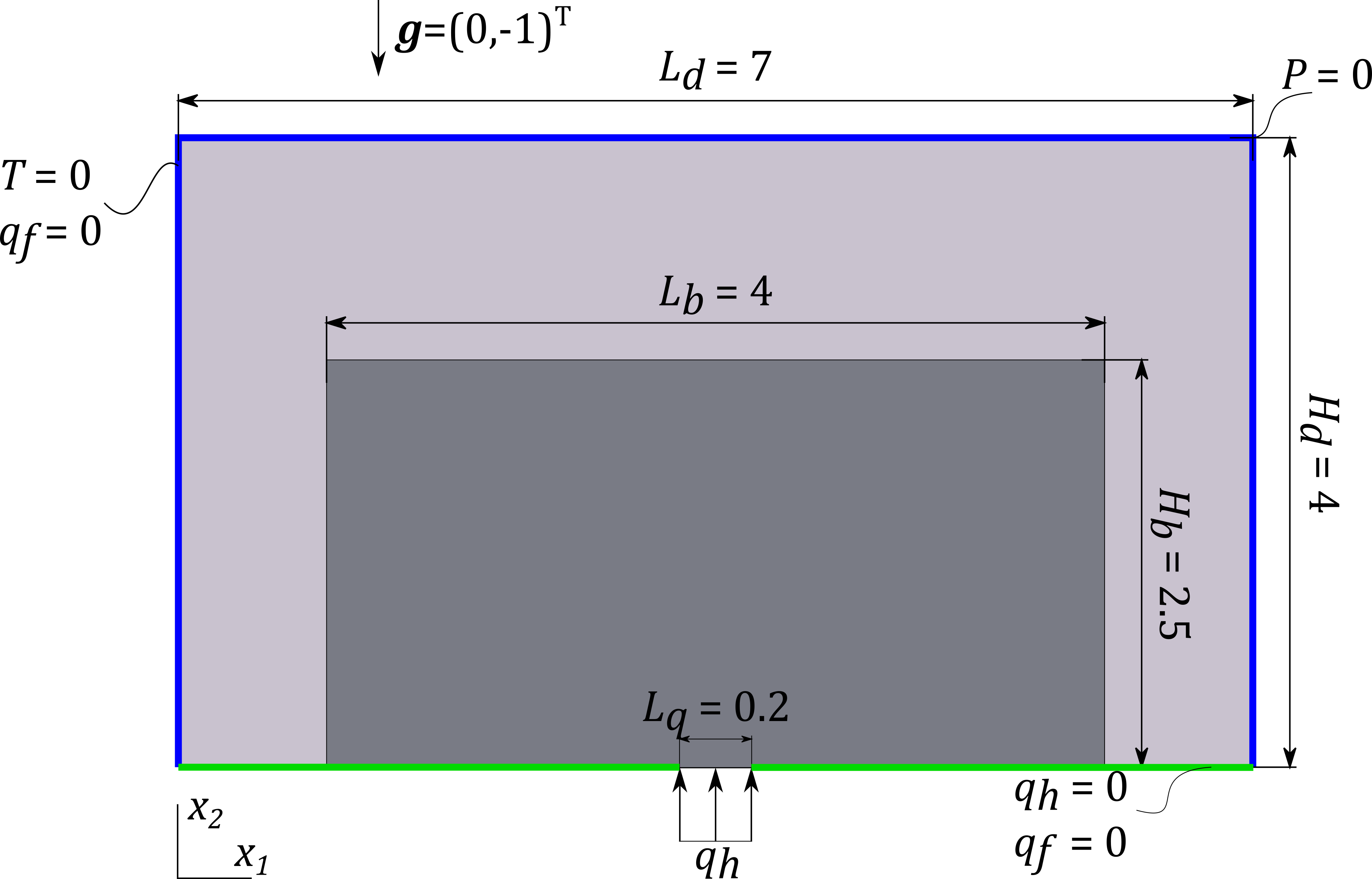
Figure 1: Domain used for comparison of reduced- and full-order models. Light gray denotes fluid domain while darker gray indicates solid domain. No fluid flow is allowed across the outer boundary $(q_{f}=0)$.

The presented potential flow model is intended to approximate flows governed by the full Navier-Stokes equations. The introduction of the reduced-order material property, $\bar{\mu}$, requires tuning in order to use the reduced-order model. Thus, it is of interest to investigate the difference between the results achieved using the proposed reduced-order model and the full-order model. For the full-order model, the laminar flow module of COMSOL Multiphysics 5.3 is used. The Brinkman term is added by appending a volume force to the Navier-Stokes equations. The problem used for tuning is shown in Fig. 1.

A box of solid material (dark gray) is located in a closed cavity surrounded by fluid (light gray). The domain has unit out-of-plane thickness, i.e. $t_{\textrm{D}}=1$. A distributed heat flux of size $q_{\textrm{h}}=110$ is applied to the center part of the bottom boundary. The vertical and top walls are subject to temperature conditions $T=0$, while the lower wall is insulated, $-k\frac{\partial T}{\partial x_{i}}n_{i}=0$. A reference pressure $P=0$ is applied at the top right corner. The gravitational acceleration is vertical and of size $\mathbf{g}=\{0,-1\}^{\textrm{T}}$ and the thermal expansion coefficient is $\beta=100$, yielding an effective $\textrm{Gr}=6400$. The domain is discretized using 280x160 square elements. The natural boundary condition for the potential flow model is no flux, i.e. a no-penetration slip condition on the velocities. Hence, in order to ensure maximum comparability, the outer walls in the full-order model are modeled as no-penetration slip-boundaries, i.e. $u_{i}n_{i}=0$. The material properties used are shown in Tab. 1. Ideally, the velocities inside the solid should be zero, requiring $\bar{\mu}_{s}=\infty$. However, numerically this is not practical and thus a high, but finite, value is chosen, $\bar{\mu}_{s}=10^{7}$. Correspondingly, in the NSB model, the Brinkman coefficient is set to 0 in the fluid, $\alpha_{f}=0$, and to a high, but finite, number in the solid, $\alpha_{s}=10^{7}$. Furthermore, the fluid viscosity in the reference NSB model is set to 1, $\mu=1$.

Table 1: Material properties for the calibration example.

	$k$	$\bar{\mu}$	$\beta$	$c_{p}$	$\rho_{0}$
Solid	100	$10^{7}$	1	1	1
Fluid	1	variable	1	1	1

A calibration process is conducted to find the value of $\bar{\mu}_{f}$, such that the temperature results in the best fit between the reduced-order and full-order models. The choice of using the temperature field as a quality measure is because this is the field of interest in the optimization, rather than the flow field directly. The value has been identified by minimizing the least-squares error of the temperature DOFs using the two models, i.e. $1/N_{dof}\sum(T_{NSB}-T_{ROM})^{2}$. A plot is shown in Fig. 2, from which a value of $\frac{1}{\bar{\mu}_{f}}=0.09$ is chosen based on the figure of merit. Fig. 3 also shows that a qualitatively good comparison is obtained. Fig. 3a and 3b show the temperature fields and streamlines for the two models. From this it is seen that the reduced-order model produces qualitatively similar results when tuned appropriately.

Velocity magnitudes are illustrated in Figs. 3c and 3d and are seen to be generally in the same range. However, major discrepancies are observed at the fluid-solid interface, which is due to the lack of a viscous boundary layer in the potential flow model. Thus, the local flow velocity, as well as the width of the recirculation cells, at the sides are over-predicted by the potential flow model.

The chosen value of $\bar{\mu}_{f}$ is assumed to be constant with respect to convection/diffusion dominance and will be used for other Grashof numbers as well. It is the authors experience that the best $\bar{\mu}_{f}$ is mostly dependent on problem geometry for the problems investigated herein.

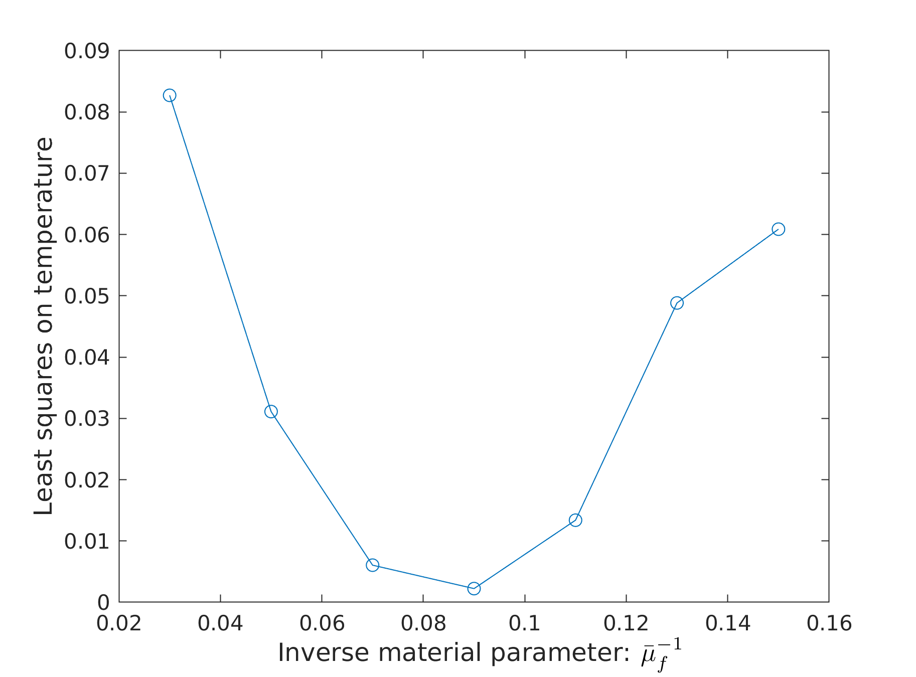
Figure 2: Least-squares error of temperature DOFs in the potential flow and NSB models for varying $\bar{\mu}_{f}$, while simulating the problem given in Fig. 1.

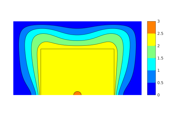
(a) Reduced-order, temperature

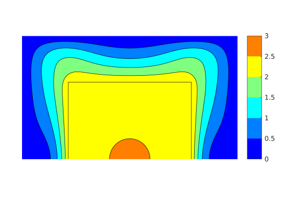
(b) Navier-Stokes-Brinkman, temperature

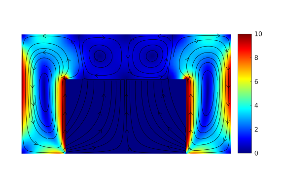
(c) Reduced-order, velocity

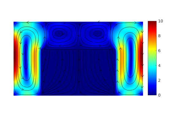
(d) Navier-Stokes-Brinkman, velocity

Figure 3: Comparison of state fields for the test problem of 1 between the potential flow and NSB models. Upper row shows temperatures and streamlines, while bottom row shows the velocity magnitude.

6 Results

6.1 Heat Sink

Topology optimization is now applied to the problem depicted in Fig. 1. The dark gray area is considered as the design domain. The problem was originally treated by Alexandersen et al (2014), although with no-slip boundary conditions at the outer walls. Only half the domain is modeled due to symmetry. The model domain is discretized with 140x160 square elements. The filter radius is set to $r_{\textrm{min}}=0.06$, corresponding to 2.4 elements. The allowed solid volume fraction is $50\%$ of the design domain.

In order to compare to the results of Alexandersen et al (2014), the problem is investigated with $\textrm{Pr}=1$ and at varying Grashof numbers. Note that the choice of $\textrm{Pr}=1$ and all material parameters set to 1, except $k_{s}=100$ and a varying $\beta$, corresponds to $\textrm{Gr}=\textrm{Ra}=\beta H^{3}$ cf. (27). The treated problem only has a single prescribed temperature, which makes it difficult to determine the Grashof-number a priori. Thus, an a priori Grashof-number is defined assuming a temperature difference of $\Delta T=1$. This a priori Grashof-number is solely used to scale the convective to diffusive heat transfer. The physical Grashof-number can a posteriori be determined based on the resulting temperature field (Alexandersen et al (2016)).

Three cases are considered with a priori Grashof numbers $\textrm{Gr}=\{640,3200,6400\}$. The lowest case yields a solution which is heavily diffusion-dominated, while the latter yields a case in which convective heat transfer plays a significant role. The resulting designs are presented in Fig. 4. For the diffusion-dominated case of $\textrm{Gr}=640$, shown in Fig. 4(a), the optimized design shows significant branching extending towards the boundary of the design domain. The design shows little tendency to accomodate the flow. Optimizing for a problem with no flow yielded qualitativly similar designs. Increasing the Grashof-number to Gr = 3200 removes most of the branching at the vertical design domain boundaries, see Fig. 4(b), allowing for more heat to be convected away. For the case of $\textrm{Gr}=6400$, shown in Fig. 4(c), all branching has disappeared and the obtained designs has smoothly-varying walls.

The observed design trend is exactly the same as seen when using the full Navier-Stokes model (Alexandersen et al, 2014). The design starts with significant branching for the diffusion-dominated problem and then branching becomes less dominant as convection increases. In fact, comparing one-to-one with the designs obtained by Alexandersen et al (2014), the resemblence is surprisingly good. Although extremely similar, there are subtle differences. For example, the design for $\textrm{Gr}=6400$ (Fig. 4(c)) features a less smooth surface with a deeper dimple along the rightmost interface. These differences are most likely due to the lack of viscous friction close to the design interfaces, in the potential flow model.

To evaluate the performance of each design, a cross-check of the final objective function is conducted. The thermal compliance is evaluated for each design at each flow state. The thermal compliance is evaluated at the final penalization factors, $p_{k}=16$ and $p_{\bar{\mu}}=20$, and the results are listed in Tab. 2. The cross-check confirms that the designs, relative to each other, are best at the Grashof number at which they were optimized.

Table 2: Cross-check of design performance . All designs are evaluated at $\textrm{Gr}={640,3200,6400}$ and the related thermal compliance ($[\times 10^{-1}]$) is stated in the table. Bold text indicates best performance for a given setting (column). Designs evaluated using $p_{k}=16$ and $p_{\kappa}=20$.

	Evaluated at Gr
Designed for Gr	640	3200	6400
$640$	8.06	7.36	6.42
$3200$	8.28	7.30	6.22
$6400$	8.80	7.36	5.94

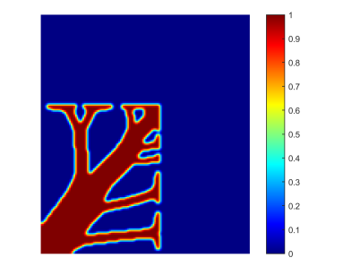
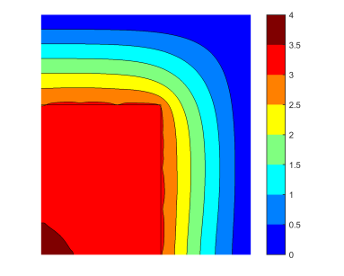
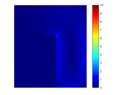
$\textrm{Gr}=640$

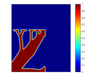
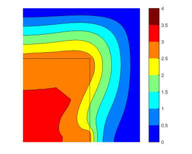
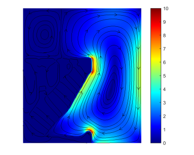
$\textrm{Gr}=3200$

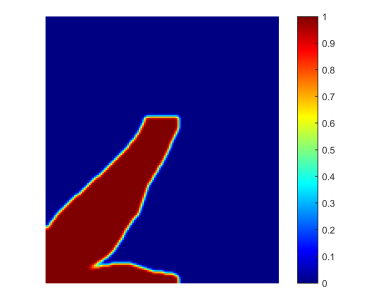
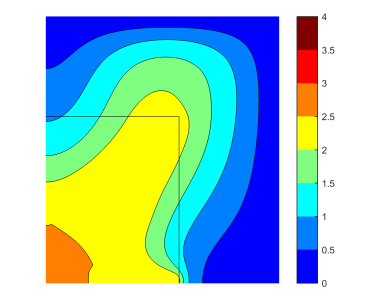
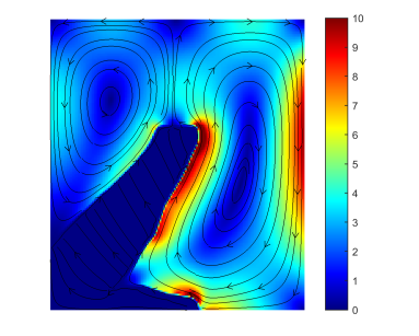
$\textrm{Gr}=6400$

Figure 4: Design, temperature and velocity fields for three cases obtained using the reduced-order model.

6.2 Comparison of performance under the full-order model

The obtained designs are tested using the full-order flow model, where designs are thresholded, to obtain truly black/white designs, using a smooth isocontour of the design field. The threshold value is set such that design values satisfying $\gamma\geq 0.1$ are solid, while design values satisfying $\gamma<0.1$ are fluid. The thresholded designs along with temperature and velocity profiles are shown in Fig. 5.

For the reevaluation, no-slip conditions are used on the outer walls, as this is considered the true reference case (Alexandersen et al, 2014). The stream profiles are qualitatively similar to those produced by the reduced-order model, with an equal number of vortices produced.

A cross-check of the objective functions is shown in Tab. 3. It can be seen that the cross-check is still passed for the thresholded designs. The values using the Navier-Stokes flow model are slightly higher than when using the potential flow model, most likely due to a combined effect of the design thresholding and the no-slip conditions along the interface. Furthermore, compared to the reference results presented by Alexandersen et al (2014), the reduced-order results give a slightly lower thermal compliance. This is likely due to convergence to local minima and small differences in the implementations and the thresholding procedures. The maximum temperature shows that the true Grashof numbers are a factor of 3 to 4 higher than the a priori computed.

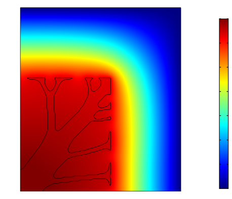
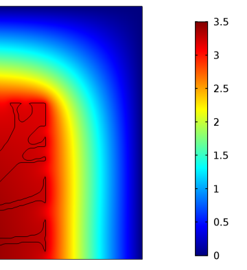
(a) Temperature, $\textrm{Gr}=640$

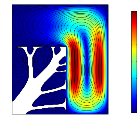
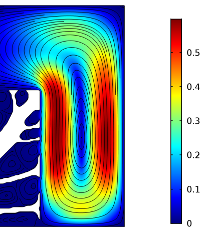
(b) Velocity, $\textrm{Gr}=640$

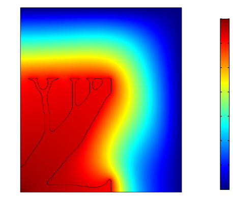
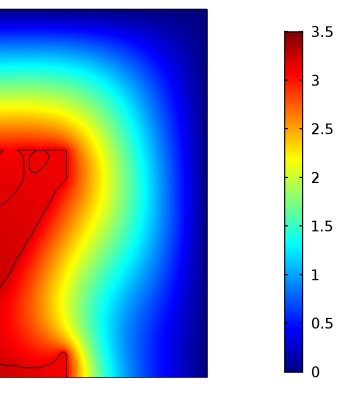
(c) Temperature, $\textrm{Gr}=3200$

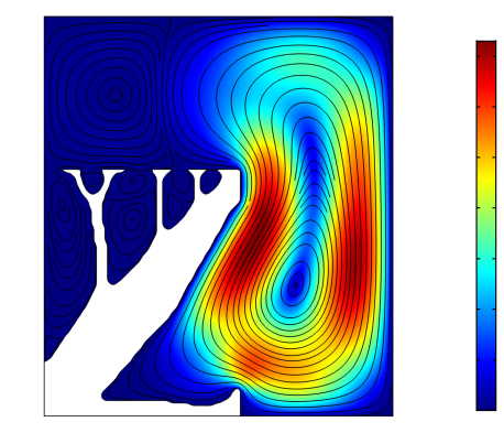
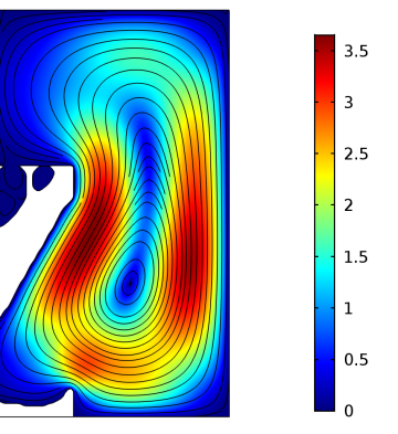
(d) Velocity, $\textrm{Gr}=3200$

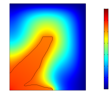
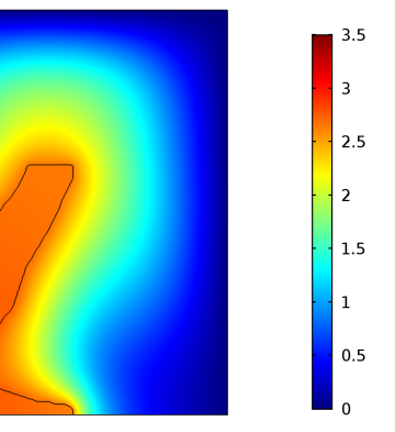
(e) Temperature, $\textrm{Gr}=6400$

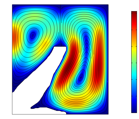
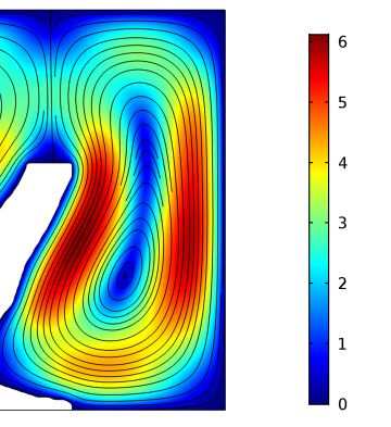
(f) Velocity, $\textrm{Gr}=6400$

Figure 5: Heat sink results when modeling the fluid flow using a NS flow model. Note that no-slip walls were used at the domain boundaries.

Table 3: Thermal compliance values ($[\times 10^{-1}]$) from the NS model with no-slip conditions at all solid-fluid interfaces. $\Delta T_{max}$ is the maximum observed temperature difference.

	Evaluated at Gr			$\Delta T_{max}$ at Gr
Designed for Gr	640	3200	6400	640	3200	6400
$640$	8.12	7.82	7.24	3.7	3.6	3.3
$3200$	8.38	7.78	7.00	3.8	3.6	3.2
$6400$	8.94	7.88	6.62	4.1	3.6	3.0

6.3 Comparison to naive simplified convection model

The proposed reduced-order model is further compared to using a naive simplified convection model based on Newton’s law of cooling, with a constant convection coefficient on the solid-fluid interface (Alexandersen (2011); Coffin and Maute (2016b); Zhou et al (2016); Lazarov et al (2014)). This model does not model the flow at all and the specific approach is described in Appendix B. The convection coefficient for the three Grashof numbers are calculated from COMSOL models of the reference designs from (Alexandersen et al, 2014) using the full Navier-Stokes flow model, by computing the surface average of the local convection coefficient:

$$\bar{h}=\frac{1}{A_{fs}}\int_{\Gamma_{fs}}\frac{q_{n}}{T}ds$$ (42)

where $\bar{h}$ is the average convection coefficient, $A_{fs}$ is the area of the fluid-solid interface ($\Gamma_{fs}$) and $q_{n}$ is the normal flux at the interface.

Table 4: Non-dimensional effective convection coefficients for the three Grashof numbers, calculated from the full-order model for the reference designs from (Alexandersen et al, 2014).

Grashof	640	3200	6400
$\bar{h}$	0.17883	0.27820	0.76345

Table 5: Final thermal compliance values ($[\times 10^{-1}]$) for the optimised design using naive simplified convection model, evaluated using the simplified and full-order models for the three Grashof numbers. The average convection coefficient calculated using the full-order model is also shown.

Gr	640	3200	6400
Simplified conv. model	6.9825	4.2579	2.4703
Full model	7.9778	7.8008	7.2695
$\bar{h}$	0.16089	0.14301	0.15703

The non-dimensional convection coefficient for the three cases is shown in Tab. 4. These values are then used in the optimisation procedure using the simplified convection model. The obtained designs are shown in Fig. 6. It can be seen that the obtained designs are significantly different from those using the two flow models. The designs contain closed cavities and small-scale features. The internal cavities appear due to the global nature of the simplified convection model, where the convective boundary condition is applied on all fluid-solid interfaces and does not discriminate between internal and external surfaces. Similarly, the small-scale features are attractive due to a combination of the problem being purely conductive (although with a convection boundary condition) and the fact that more surface area yields better heat transfer. The obtained designs are imported into COMSOL and evaluated using the full Navier-Stokes flow model and the results of this analysis is shown in Fig. 7. As expected, it is clear that the fluid in the internal parts of the heat sinks (partially- and fully-closed cavities) is moving at near zero velocities and, thus, almost no cenvective heat transfer is taking place. This is further exemplified by Fig. 8, which shows a close-up of the velocities in the internal (partially- and fully-closed) cavities for the $\textrm{Gr}=6400$ design, when analysed using the full-order model. Here it can be seen, that although convection cells do form due to temperature variations in the solid, the resulting velocities are significantly lower than those of the outer flow due to the temperature variations being very small. The thermal compliance values using both the simplified convection model and the full Navier-Stokes models are presented in Tab. 5. The effective convection coefficient calculated using the full-order model is also shown. By comparing the thermal compliance values using the simplified and full-order models in Tab. 5, it is clear that the heat transfer is vastly over-predicted using the simplified convection model. Furthermore, it can be seen that all three designs perform more or less similarly when evaluated using the full Navier-Stokes model. However, using the simplified convection model, the higher the Grashof number / convection coefficient, the more over-predicted the heat transfer is due to internal cavities. The fact that the convective heat transfer is vastly over-estimated, is further illustrated by comparing the actual effective convection coefficient values in the bottom row of Tab. 5 with the original values in Tab. 4.

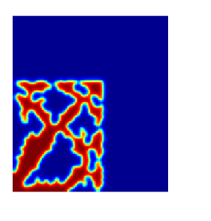
(a) $\textrm{Gr}=640$

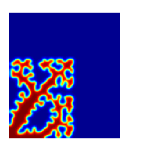
(b) $\textrm{Gr}=3200$

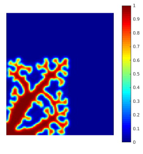
(c) $\textrm{Gr}=6400$

Figure 6: Heat sink designs obtained using the simplified convection boundary model.

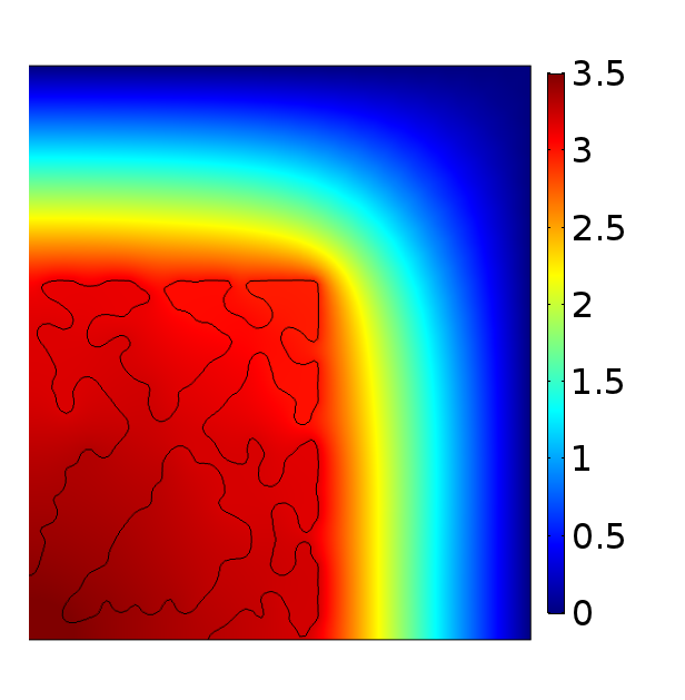
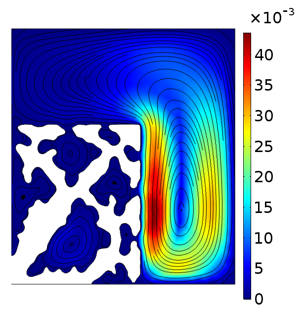
(a) $\textrm{Gr}=640$

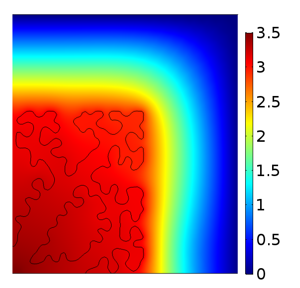
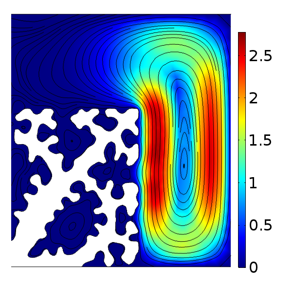
(b) $\textrm{Gr}=640$

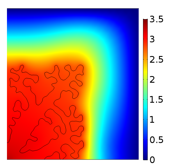
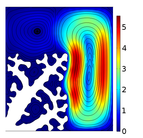
(c) $\textrm{Gr}=6400$

Figure 7: Heat sinks designed using the simplified convection boundary model evaluated using the full NS model. Left column: Temperature distribution. Right column: Velocity magnitude and streamlines.

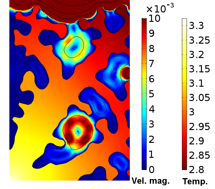
Figure 8: Close-up of the very low-velocity convection cells inside close cavities for the $\textrm{Gr}=6400$ simplified model design. The velocity field and the solid temperature distribution are shown using two seperate color schemes and scales.

6.4 Centrally heated domain

The second example considers a rectangular cavity as shown in Fig. 9. The vertical cavity walls are assumed adiabatic except, for the centre part of the left wall which is heated by a constant heat flux $q_{h}=3$. The top and bottom are assumed isothermal $T=0$. All boundaries are assumed closed with slip condition $u_{i}n_{i}=0$ and the pressure in the top right corner is constrained to zero. The gravity is pointing downwards $g=(0,-1)^{T}$. The domain is discretised using $120\times 240$ elements using a filter with radius $r_{\textrm{min}}=0.08$ ($2.4$ elements).

The objective is to minimize the thermal compliance in the domain subject to a volume constraint for solid material of $30\%$ of the design domain. In the first example, a large part of the heat was transported from the structure to the right vertical wall by convection. In this example, the vertical wall is insulated forcing the optimizer to design optimized cooling through two horizontal boundaries which is more challenging. The low temperature of the top boundary can be utilized with relative ease while the low temperature of the bottom boundary is more difficult to utilize as it requires that hot fluid is pushed downwards while relatively colder fluid must be pushed upwards. This results in separate diffusion and convection dominated areas as will be discussed below.

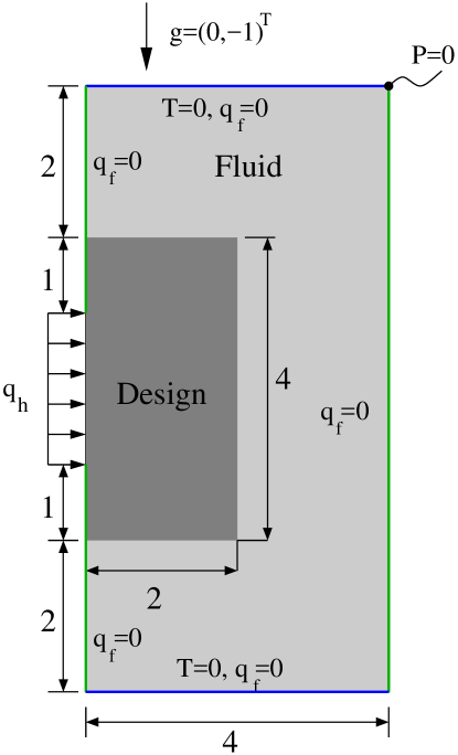
Figure 9: Rectangular closed cavity heated through the centre part of the left otherwise insulated boundary. Right boundary is insulated while top and bottom are isothermal, $T=0$. All boundaries are modeled as slip $u_{i}n_{i}=0$ and the pressure is constrained $p=0$ in the lower left corner.

The results in this section are obtained using only the first penalization step in the previously mentioned continuation scheme and an initial uniform material distribution of $10\%$ solid in the design domain. The continuation has been omitted as the level of discreteness in the solution after the first penalization step was satisfactory.

The parameter $\bar{\mu}$ has been obtained using the same method as for the previous example. The design domain is considered solid and the temperature distribution is obtained both by the NSB and the reduced-order model. The value of $\bar{\mu}$ that minimizes the least squares temperature difference was found to be $\bar{\mu}^{-1}=0.15$ under the condition $\textrm{Gr}=51200$ using a sweep with intervals of $\Delta(\bar{\mu}^{-1})=0.02$.

The optimized designs for the thermal expansion coefficients $\beta=\{10,50,100\}$ are shown in Fig. 10. As in the previous example, material parameters are chosen such that $\textrm{Gr}=\textrm{Ra}=\beta H^{3}$ which yields $\textrm{Gr}=\{5120,10240,51200\}$. It is clear that for the lowest Grashof number the conductive transport is dominating, which is clear from the symmetric design with branching and the corresponding temperature plot. The velocities are moderate and stay below 1, having the highest magnitude at the vertical interface between heat sink and fluid. Increasing the Grashof number to $\textrm{Gr}=10240$ and even further to $\textrm{Gr}=51200$ results in a very convection influenced design, at least for the upper part of the design domain. A heat sink that allows a large convection roll to form at the top part appears. The lower part of the heat sink has more in common with the previous diffusion dominated design, where branching is formed to support the heat diffusion away from the source towards the cold bottom boundary. The heat sink is divided centrally by a small fluid spacing. This insulates the bottom part from the top and restricts the temperature in this part of the sink. The bottom part is cooled primarily by diffusion at the bottom face and by convection at the upper face. At this face the heat is exchanged to the cold fluid which makes the fluid gain velocity. Further up, in the top part of the heat sink, the fluid momentum is boosted by the higher temperature in the top part of the heat sink. This difference in heat transport is also visible from the velocity magnitude plot, which clearly shows that the velocities are in general low in the bottom part of the domain where diffusion dominates. The velocity is high at the sink’s vertical interface with the fluid domain, where the hot sink is heating the fluid and making it flow in the direction of gravity. The largest velocities are obtained near the upper hot part of the heat sink.

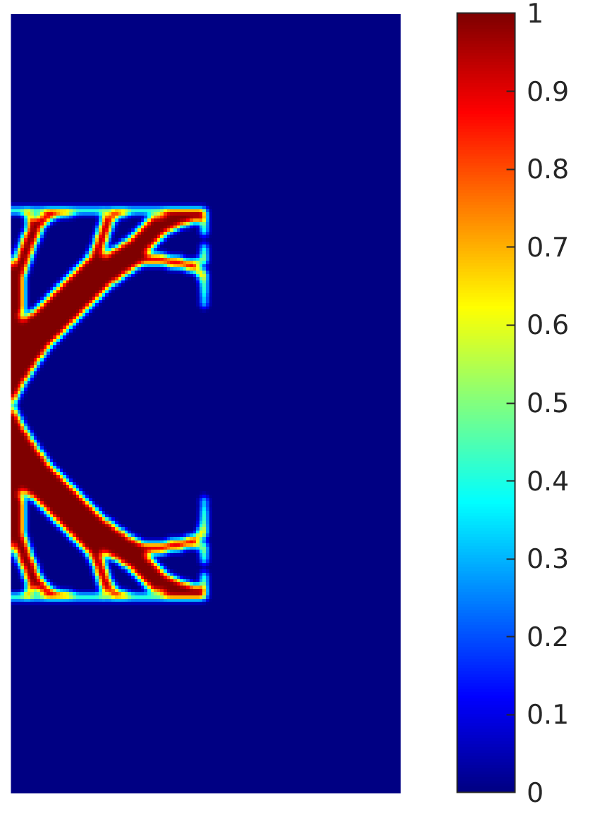
(a) Design, $\textrm{Gr}=5120$

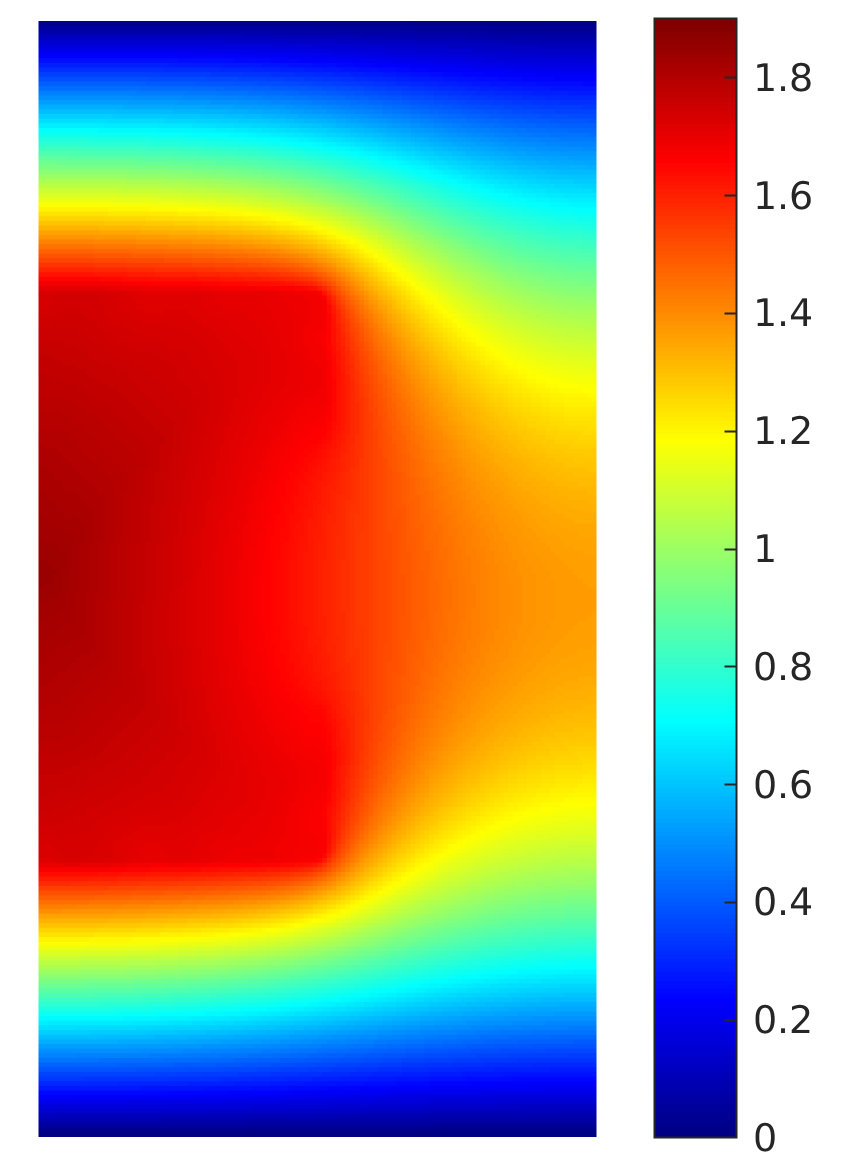
(b) Temperature, $\textrm{Gr}=5120$

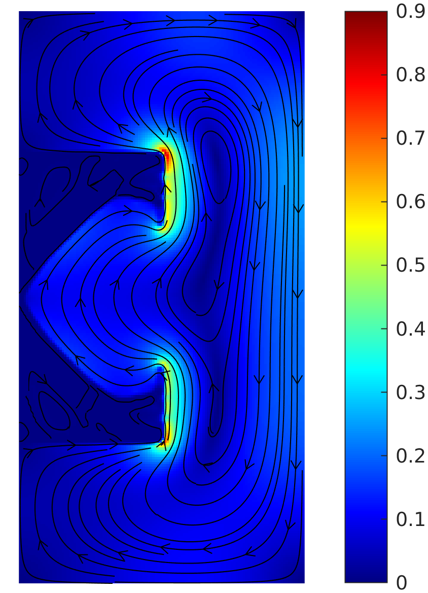
(c) Velocity, $\textrm{Gr}=5120$

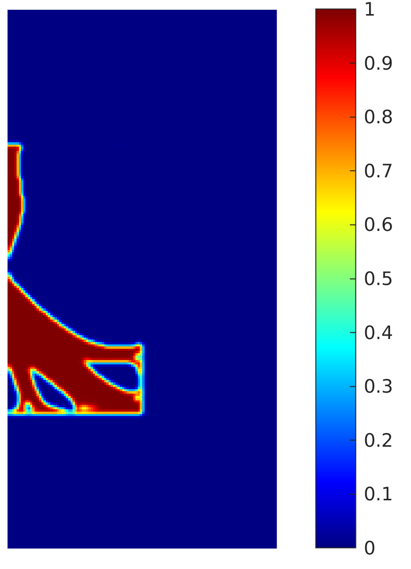
(d) Design, $\textrm{Gr}=10240$

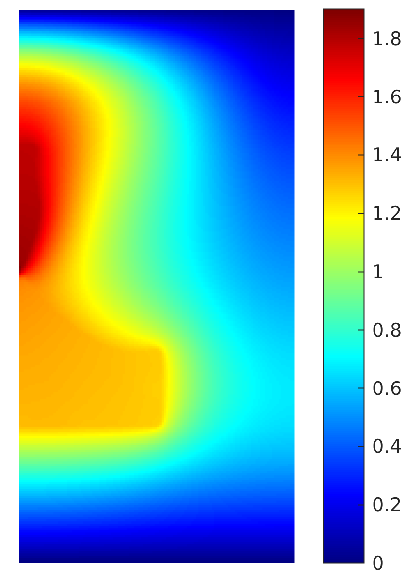
(e) Temperature, $\textrm{Gr}=10240$

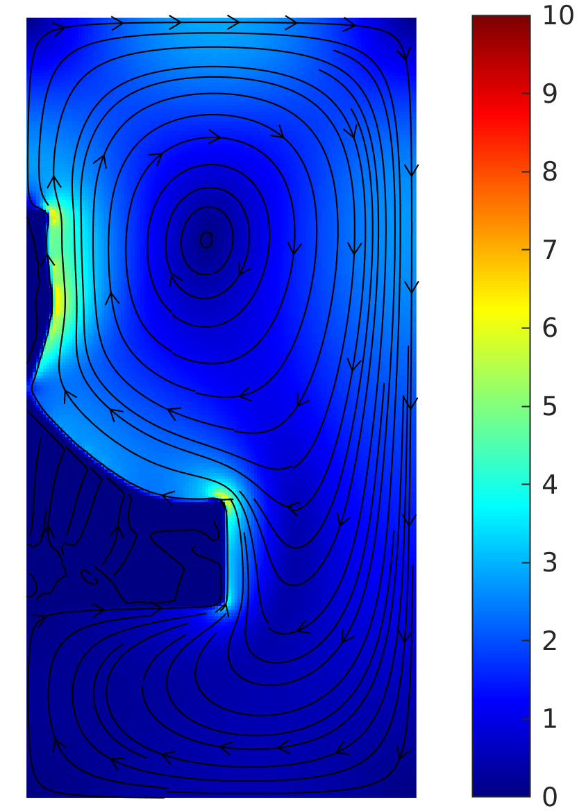
(f) Velocity, $\textrm{Gr}=10240$

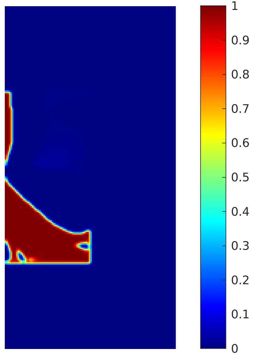
(g) Design, $\textrm{Gr}=51200$

(h) Temperature, $\textrm{Gr}=51200$

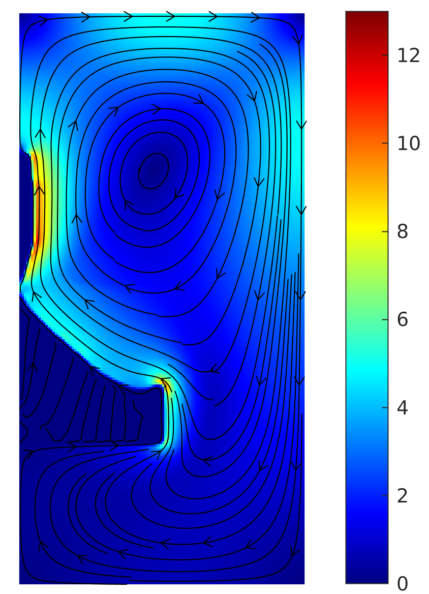
(i) Velocity, $\textrm{Gr}=51200$

Figure 10: Optimized designs and state plots for Grashof numbers $\textrm{Gr}=\{5120,10240,51200\}$. Note that velocity color scale varies for increased visual reading.

	Compliance at Gr			$\Delta T_{max}$ at Gr
Designed at Gr	5120	10240	51200	5120	10240	51200
5120	10.75	10.07	8.50	1.85	1.74	1.48
10240	12.54	9.24	7.52	2.42	1.88	1.55
51200	12.83	9.27	7.48	2.54	1.92	1.56

Table 6: Performance for optimized designs evaluated under all conditions. The Grashof numbers refer to an assumed temperature difference $\Delta T=1$. The maximum temperature is for all cases identified slightly above the centre of the heat source boundary.

The performance of the optimized designs can be compared in-between the different designs and values are listed in Tab. 6. Each of the designs perform best at their respective design condition. The maximum temperature reveals that the true Grashof number is about the double value of the a priori computed.

The designs obtained by the reduced-order model can be compared to those obtained by a full NSB model in order to verify that the obtained designs are somewhat similar and the design trend stepping from a diffusion dominated to a convection dominated setting results in comparable designs. Such designs are shown in Fig. 11 and it is clear that the results match very well for the diffusion-dominated design.

The convection-dominated design differs slightly as the NSB design seems to facilitate a smooth low-curvature flow path at the fluid-solid interface of the heat sink. This is different from the reduced order design, where the curvature is steeper, as was also observed for the first example. This may be attributed to the neglected viscous dissipation, which favours smooth directional changes. In the designs obtained for $\textrm{Gr}=10240$ and $\textrm{Gr}=51200$, a small amount of material is left near the eye of the convection cell and the reason for placing it here is attributed purely to minor flow guidance effects as the conductive properties are poorly exploited at this position. It is likewise possible to achieve such small amounts of material at this location using the reduced-order model. However, it is the authors experience that the occurrence depends on initial material distribution and penalization scheme and has limited influence on the end performance.

(a) $\textrm{Gr}=5120$

(b) $\textrm{Gr}=10240$

(c) $\textrm{Gr}=51200$

Figure 11: Comparative designs obtained using the fully coupled Navier-Stokes-Brinkman equations for the same Grashof numbers $\textrm{Gr}=\{5120,10240,51200\}$. Designs obtained using a MATLAB-COMSOL implementation of the formulation used in Alexandersen et al (2014). The objective values read $\phi_{5120}=11.10$, $\phi_{10240}=7.94$, $\phi_{51200}=6.93$

The obtained designs from the reduced-order model have been thresholded at $\gamma=0.5$, smoothed using an isocontour and exported to COMSOL. Using $\gamma=0.5$ as the threshold value yields exported designs with volume fractions close to the optimized. The visualisations of the results are shown in Fig. 12 and the obtained performance, solid volume fraction and maximum temperatures are listed in Tab. 7 for all conditions. Here the boundary conditions have been maintained as slip boundaries as for the reduced order model. This also applies to the solid-fluid interface.

For the lowest Grashof numbers the temperature and velocity distributions are very similar which is attributed to the diffusion dominance. The velocities show the expected behaviour and the streamlines of the two models are similar. The colours show that the local maximum velocity at the fluid-solid interface differs from the NS model where the maximum is attained at a certain distance from the solid due to viscous boundary effects.

When the Grashof number is increased it is seen that the difference in the temperature distributions increases. The localisation of the velocity seems to limit the ability to convect the fluid. Comparing the flow speed for $\textrm{Gr}=10240$, it is evident that the maximum velocity near the top part of the heat sink for both models is around 6-7. As the high velocity area in the full model is much more distributed, this also means that more momentum is available which in turn convects more heat resulting in a more mushroom-shaped thermal plume. This also applies to the $\textrm{Gr}=51200$ case where the plume is increasingly mushroom-shaped, but still lacks momentum in comparison to the full model. For all cases, the diffusion dominated behaviour at the bottom of the domain seems similar for both models.

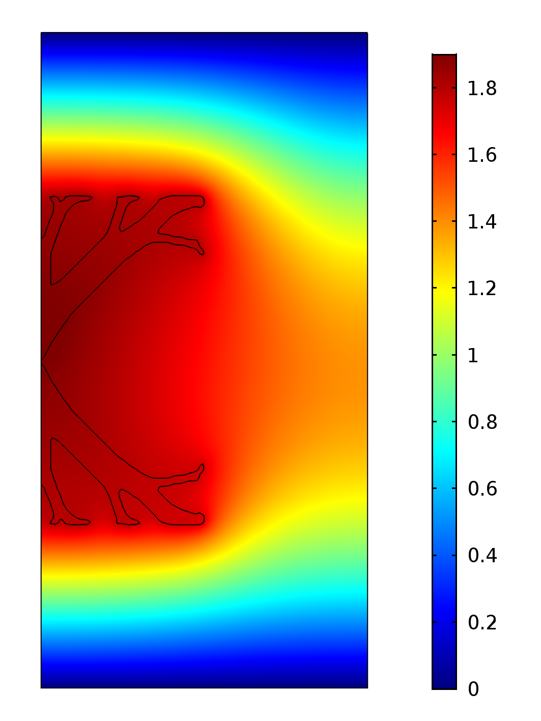
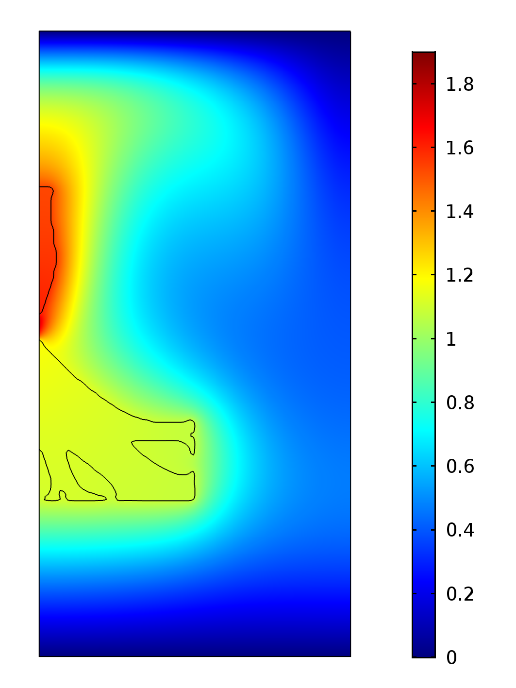
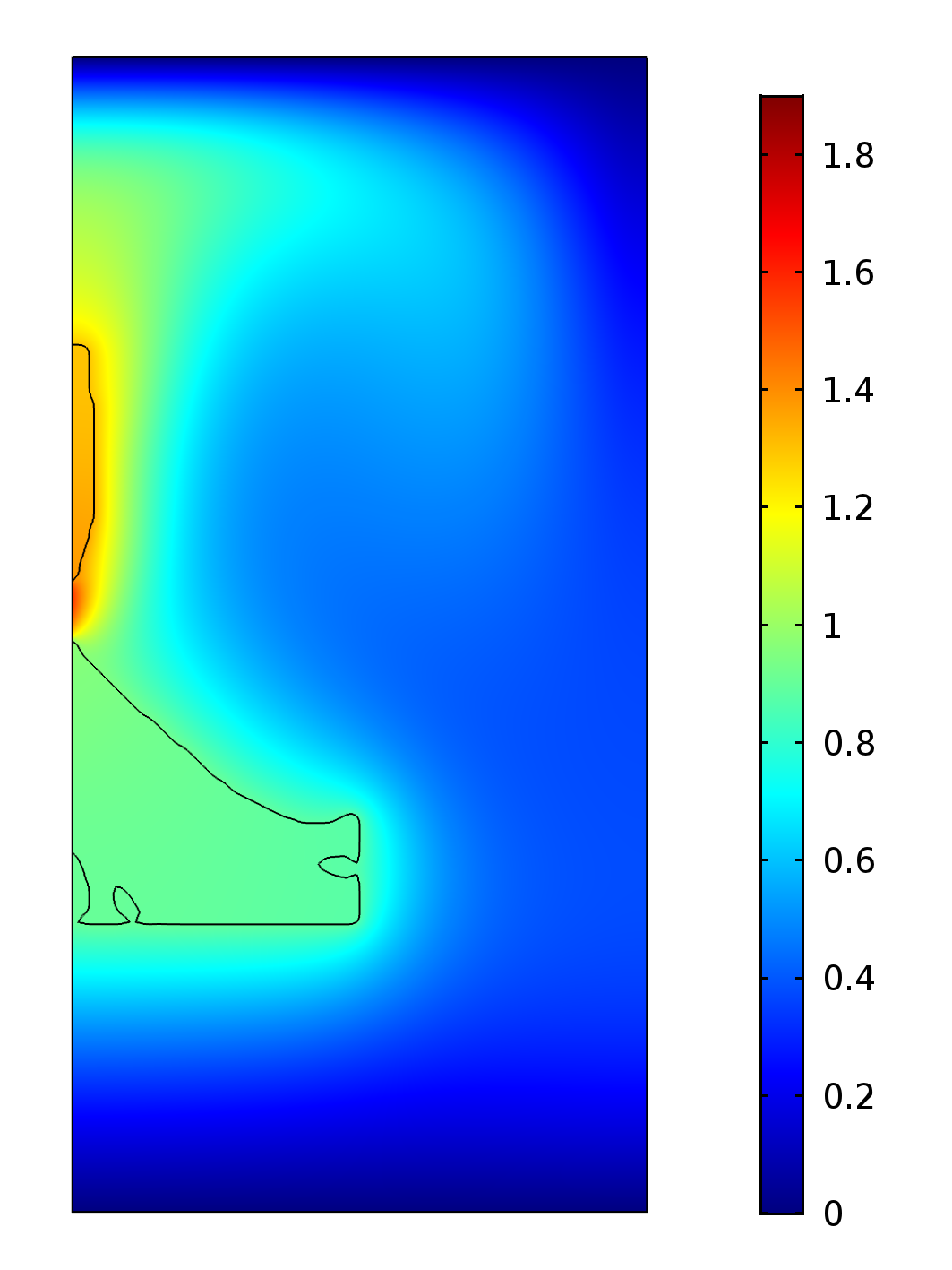
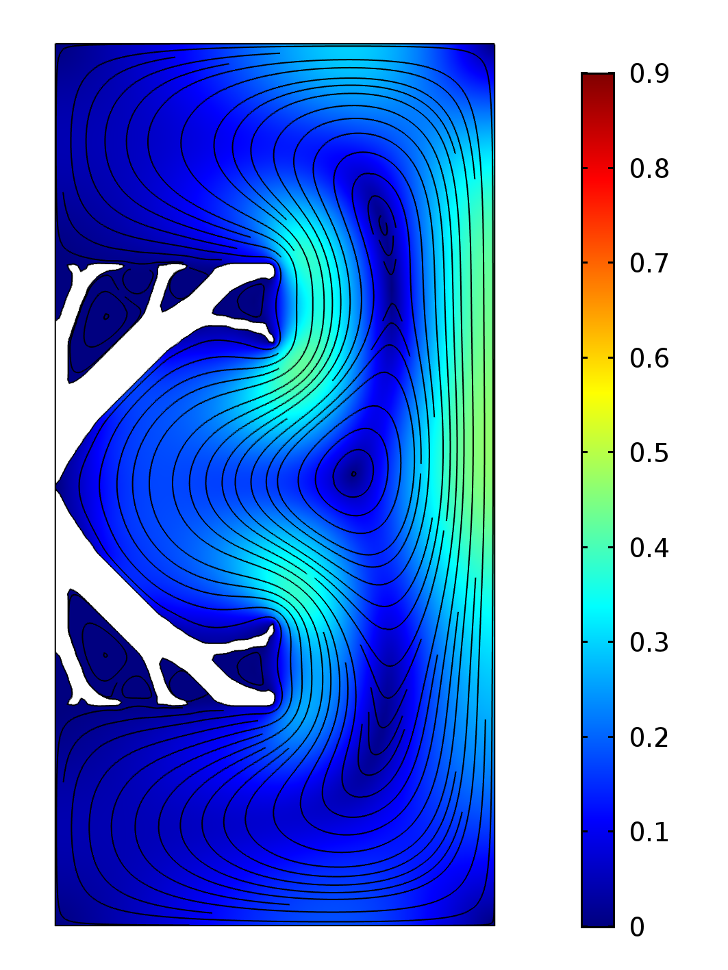
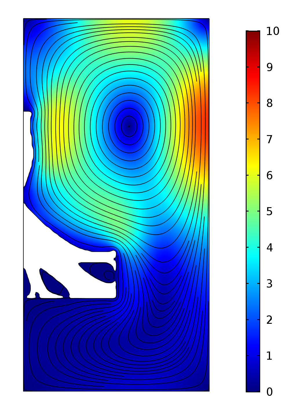
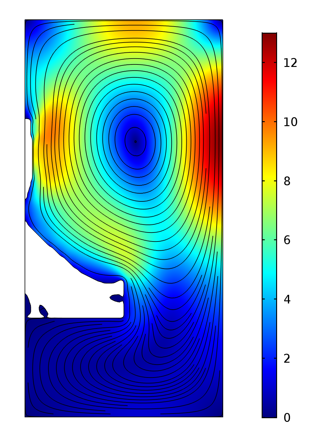
Figure 12: Reevaluation of designs using COMSOL Multiphysics 5.3. Designs thresholded at $\gamma=0.5$ and extracted using and isocontour. All boundaries are subject to the slip condition. Top row: Temperature plots. Bottom row: Velocity magnitude and streamlines. Temperature and velocity ranges correspond to Fig. 10

	Evaluated at Gr				$\Delta T_{max}$ at Gr
Designed for Gr	5120	10240	51200	Solid vol.frac.	5120	10240	51200
5120	11.36	10.11	8.52	0.287	1.93	1.77	1.49
10240	11.31	8.24	7.27	0.296	2.33	1.76	1.58
51200	11.17	8.07	7.09	0.294	2.36	1.77	1.58

Table 7: Performance for reevaluated designs using design extraction and full NS model cf. Fig. 12. The volume fraction of the extracted solid wrt. design domain is given. All designs are originally attaining the 0.3 limit.

The post processed performance listed in Tab. 7 shows that the thresholded and smoothed $\textrm{Gr}=51200$ design outperform all the others using full NS modeling. However, it must be noted that the difference in thermal compliance is very small, in the order of $2\%$ if one compares the performance of a design optimized at a certain setting with that obtained using the “$\textrm{Gr}=51200$ design“ evaluated at that setting. This small difference may of course be due to the lower fidelity of the reduced-order model and the tuning hereof, but may also be a consequence of the better geometry representation obtained using a smoothed geometry represented in a body-fitted mesh.

7 Discussion and conclusions

The paper has demonstrated a novel method for order reduction of models for optimization of natural convection problems. The reduction in dimensionality from the Navier-Stokes equations to a potential flow model has been shown to be efficient and work relatively well as a vehicle for the modeling of convection. The major obstacle for general applicability may be to find a suitable test case for tuning the material parameter $\bar{\mu}$ to yield representative state fields under different conditions and during design evolution. The lower computational complexity of the reduced-order model has shown to speed up the topology optimization design procedure for fully coupled natural buoyancy problems.

The obtained designs have been compared to those obtained using the full model and the general tendencies and performance is maintained in high-fidelity simulations. Another challenge of employing this model is clearly the lack of a boundary layer, which tends to overpredict local velocities near the boundary, while underpredicitng those further away. In the second example, this resulted in the reduced-order model to underpredict the convection and thus predict a slightly lower performance. For other cases it may be opposite, e.g. in the case of narrow channels in the design, which may cause overprediction of the convective performance in the reduced-order model due to the lack of viscous friction.

In comparison to the model utilizing Newton’s law of cooling, which is one step further down the order-reduction-path, the potential flow model is superior in predicting convection surfaces, as it does include the ability to model the natural convection in narrow and closed regions of the heat sink, which is clearly a problem for the simplified convection model.

The presented reduced-order model enables designers to shorten the computational time for design synthesis. The obtained designs come close to those of a full Navier-Stokes-Brinkman model and may be postprocessed using CAD directly or used as a close-to-optimal initial design for a method that models the fully coupled Navier-Stokes equations.

Acknowledgements The work has been partly funded by the TopTEN project granted by Independent Research Fund Denmark. The authors would like to thank the TopOpt group for fruitfull discussions.

Appendix A Sensitivity analysis

The sensitivity of the objective function with respect to the design variables $\bm{\gamma}$ is determined using the adjoint sensitivity method. The objective function is augmented by the product of the residual and an adjoint vector:

$$\hat{\psi}=\psi+\bm{\lambda}^{\textrm{T}}\mathbf{R}(\mathbf{s}),$$ (43)

where $\bm{\lambda}$ is the adjoint vector.

Differentiating with respect to the design variables $\bm{\gamma}$ yields:

$$\frac{\textup{d}\hat{\psi}}{\textup{d}\bm{\gamma}}=\frac{\partial\psi}{\partial\bm{\gamma}}+\frac{\partial\psi}{\partial\mathbf{s}}\frac{\textup{d}\mathbf{s}}{\textup{d}\bm{\gamma}}+\bm{\lambda}^{\textrm{T}}\left(\frac{\partial\mathbf{R}}{\mathbf{\partial}\bm{\gamma}}+\frac{\partial\mathbf{R}}{\partial\mathbf{s}}\frac{\textup{d}\mathbf{s}}{\textup{d}\bm{\gamma}}\right)$$ (44)

The adjoint vector is chosen such that terms involving $\frac{\textup{d}\mathbf{s}}{\textup{d}\bm{\gamma}}$ are eliminated. The following adjoint problem is thus solved:

$$\bm{\lambda}^{\textrm{T}}\frac{\partial\mathbf{R}}{\partial\mathbf{s}}=\frac{\partial\phi}{\partial\mathbf{s}}$$ (45)

The matrix $\frac{\partial\mathbf{R}}{\partial\mathbf{s}}$ is recognized as the tangent matrix utilized in the Newton-Raphson algorithm which more conveniently may be determined as:

$$\frac{\partial\mathbf{R}}{\partial\mathbf{s}}=\begin{bmatrix}\frac{\partial\mathbf{R}_{p}}{\partial\mathbf{P}}&\frac{\partial\mathbf{R}_{p}}{\partial\mathbf{T}}\\ \frac{\partial\mathbf{R}_{t}}{\partial\mathbf{P}}&\frac{\partial\mathbf{R}_{t}}{\partial\mathbf{T}}\end{bmatrix}$$ (46)

When using the thermal compliance as objective function we have:

$$\frac{\partial\psi}{\partial\mathbf{s}}=\begin{pmatrix}\mathbf{0}\\ \mathbf{f}_{t}\end{pmatrix}^{\textrm{T}}$$ (47)

After solving (45) for $\bm{\lambda}$ the sensitivities can be determined as:

$$\frac{\textup{d}\psi}{\textup{d}\bm{\gamma}}=\frac{\partial\psi}{\partial\bm{\gamma}}-\bm{\lambda}^{\textrm{T}}\frac{\partial\mathbf{R}}{\partial\bm{\gamma}}=-\bm{\lambda}^{\textrm{T}}\frac{\partial\mathbf{R}}{\partial\bm{\gamma}}$$ (48)

Appendix B Simplified convection model

The simplified convection model used for comparison herein, is based on Newton’s law of cooling applied on the solid-fluid interface using a design field gradient approach. This was first presented for a density-based topology optimisation approach by (Lazarov et al, 2014). Instead of applying a design-dependent convection boundary condition on interfaces between all elements based on the jump in the physical element design field (Bruns, 2007; Alexandersen, 2011), a mathematically consistent and convergent volumetric formulation is posed based on the gradient of the physical design field. The approach can be seen as loosely equivalent to that presented for a level set approach by (Yamada et al, 2011), in that the gradient of the design field is equivalent to the gradient of the level set field, which defines the surface. For an overview of this approach, please see the work by (Alexandersen, 2011; Coffin and Maute, 2016b).

Shortly, the governing partial differential equation becomes:

$$-\frac{\partial}{\partial x_{i}}\left(k(\gamma)\frac{\partial T}{\partial x_{i}}\right)+\left\lVert\frac{\partial\gamma}{\partial x_{i}}\right\rVert_{2}h\left(T-T_{0}\right)-Q=0$$ (49)

where $h$ is the convection coefficient and in the discrete case $\left\lVert\frac{\partial\gamma}{\partial x_{i}}\right\rVert_{2}=n_{i}d\Gamma_{fs}$, with $n_{i}$ being the surface normal and $\Gamma_{fs}$ being the fluid-solid interface. For the full derivation, please see Lazarov et al (2014).

The optimization process is carried out with a continuation approach for the filter radius. The filter radius starts large to smooth out boundary effects initially and then gradually decreased using the sequence $r_{\text{min}}\in\{0.48,0.36,0.24,0.12\}$ switching after 50 iterations or when the objective functional change has been under $10^{-3}$ for 10 consecutive iterations. The final length scale is double the size of that used for the fluid model results because the simplified model favours very small features of high complexity with many internal voids. Therefore, the larger length scale results in a fairer comparison as it reduces the non-physical artifacts. The conductivity is interpolated using the modified SIMP approach, $k(\gamma)=k_{\text{min}}+(k_{s}-k_{\text{min}})\gamma^{p}$, with $k_{s}=100$, $k_{\text{min}}=10^{-6}$ and a constant penalization factor of $p=6$. The relatively high penalization factor produces better performing results, but is not necessary to yield well-defined topologies, as the surface convection term introduces automatic penalisation of intermediate densities

References

- Alexandersen (2011) Alexandersen J (2011) Topology optimisation of convection problems. B.Eng. thesis, Technical University of Denmark, DOI 10.13140/RG.2.2.24635.72485
- Alexandersen (2013) Alexandersen J (2013) Topology optimization of coupled conveciton problems. Master’s thesis, Technical University of Denmark
- Alexandersen (2016) Alexandersen J (2016) Efficient topology optimisation of multiscale and multiphysics problems. PhD thesis, Technical University of Denmark
- Alexandersen et al (2014) Alexandersen J, Aage N, Andreasen CS, Sigmund O (2014) Topology optimisation for natural convection problems. International Journal for Numerical Methods in Fluids 76(10):699–721, DOI 10.1002/fld.3954
- Alexandersen et al (2015) Alexandersen J, Sigmund O, Aage N (2015) Topology optimisation of passive coolers for light-emitting diode lamps. In: 11th World Congress on Structural and Multidisciplinary Optimization, DOI 10.13140/RG.2.1.3906.5446
- Alexandersen et al (2016) Alexandersen J, Sigmund O, Aage N (2016) Large scale three-dimensional topology optimisation of heat sinks cooled by natural convection. International Journal of Heat and Mass Transfer 100:876–891, DOI 10.1016/j.ijheatmasstransfer.2016.05.013
- Alexandersen et al (2018) Alexandersen J, Sigmund O, Meyer K, Lazarov BS (2018) Design of passive coolers for light-emitting diode lamps using topology optimisation. International Journal of Heat and Mass Transfer 122:138–149, DOI 10.1016/j.ijheatmasstransfer.2018.01.103
- Andreasen et al (2009) Andreasen CS, Gersborg AR, Sigmund O (2009) Topology optimization of microfluidic mixers. International Journal for Numerical Methods in Fluids 61(5):498–513, DOI 10.1002/fld.1964
- Angot et al (1999) Angot P, Bruneau CH, Fabrie P (1999) A penalization method to take into account obstacles in incompressible viscous flows. Numerische Mathematik 81(4):497–520, DOI 10.1007/s002110050401
- Bendsøe and Kikuchi (1988) Bendsøe MP, Kikuchi N (1988) Generating optimal topologies in structural design using a homogenization method. Computer Methods in Applied Mechanics and Engineering 71(2):197–224, DOI 10.1016/0045-7825(88)90086-2
- Bendsøe and Sigmund (2003) Bendsøe MP, Sigmund O (2003) Topology Optimization - Theory, Methods, and Applications. Springer Verlag, Berlin Heidelberg
- Borrvall and Petersson (2003) Borrvall T, Petersson J (2003) Topology optimization of fluids in Stokes flow. International Journal for Numerical Methods in Fluids 41(1):77–107, DOI 10.1002/fld.426
- Bourdin (2001) Bourdin B (2001) Filters in topology optimization. Int J Numer Meth Engng 50(9):2143–2158, DOI 10.1002/nme.116
- Brinkman (1947) Brinkman HC (1947) A Calculation of the Viscous Force Exerted By A Flowing Fluid On A Dense Swarm of Particles. Applied Scientific Research Section A-mechanics Heat Chemical Engineering Mathematical Methods 1(1):27–34
- Brooks and Hughes (1982) Brooks AN, Hughes TJ (1982) Streamline upwind/petrov-galerkin formulations for convection dominated flows with particular emphasis on the incompressible navier-stokes equations. Computer Methods in Applied Mechanics and Engineering 32(1):199 – 259, DOI 10.1016/0045-7825(82)90071-8
- Bruns (2007) Bruns TE (2007) Topology optimization of convection-dominated, steady-state heat transfer problems. International Journal of Heat and Mass Transfer 50(15-16):2859–2873, DOI 10.1016/j.ijheatmasstransfer.2007.01.039
- Bruns and Tortorelli (2001) Bruns TE, Tortorelli DA (2001) Topology optimization of non-linear elastic structures and compliant mechanisms. Computer Methods in Applied Mechanics and Engineering 190(26-27):3443–3459, DOI 10.1016/S0045-7825(00)00278-4
- Coffin and Maute (2016a) Coffin P, Maute K (2016a) A level-set method for steady-state and transient natural convection problems. Structural and Multidisciplinary Optimization 53(5):1047–1067, DOI 10.1007/s00158-015-1377-y
- Coffin and Maute (2016b) Coffin P, Maute K (2016b) Level set topology optimization of cooling and heating devices using a simplified convection model. Structural and Multidisciplinary Optimization 53(5):985–1003, DOI 10.1007/s00158-015-1343-8
- Deaton and Grandhi (2014) Deaton JD, Grandhi RV (2014) A survey of structural and multidisciplinary continuum topology optimization: post 2000. Structural and Multidisciplinary Optimization 49(1):1–38, DOI 10.1007/s00158-013-0956-z
- Dede (2009) Dede E (2009) Multiphysics topology optimization of heat transfer and fluid flow systems. In: Proceedings of the COMSOL Conference 2009 Boston
- Dilgen et al (2018) Dilgen SB, Dilgen CB, Fuhrman DR, Sigmund O, Lazarov BS (2018) Density based topology optimization of turbulent flow heat transfer systems. Structural and Multidisciplinary Optimization 57(5):1905–1918, DOI 10.1007/s00158-018-1967-6
- Donea and Huerta (2003) Donea J, Huerta A (2003) Finite Element Methods for Flow Problems. John Wiley & Sons, Ltd, Chichester, UK, DOI 10.1002/0470013826
- Donoso and Sigmund (2004) Donoso A, Sigmund O (2004) Topology optimization of multiple physics problems modelled by Poisson ’ s equation. Latin American Journal of Solids and Structures 1(2):169–189
- Dugast et al (2018) Dugast F, Favennec Y, Josset C, Fan Y, Luo L (2018) Topology optimization of thermal fluid flows with an adjoint Lattice Boltzmann Method. Journal of Computational Physics 365:376–404, DOI 10.1016/J.JCP.2018.03.040
- Evgrafov (2006) Evgrafov A (2006) Topology optimization of slightly compressible fluids. ZAMM 86(1):46–62, DOI 10.1002/zamm.200410223
- Fries and Matthies (2004) Fries TP, Matthies HG (2004) A Review of Petrov-Galerkin Stabilization Approaches and an Extension to Meshfree Methods A Review of Petrov-Galerkin Stabilization Approaches and an Extension to Meshfree Methods. Tech. rep., Institute of Scientific Computing, Technical University Braunschweig, Braunschweig
- Gersborg-Hansen et al (2005) Gersborg-Hansen A, Sigmund O, Haber R (2005) Topology optimization of channel flow problems. Structural and Multidisciplinary Optimization 30(3):181–192, DOI 10.1007/s00158-004-0508-7
- Gersborg-Hansen et al (2006) Gersborg-Hansen A, Bendsøe MP, Sigmund O (2006) Topology optimization of heat conduction problems using the finite volume method. Structural and Multidisciplinary Optimization 31(4):251–259, DOI 10.1007/s00158-005-0584-3, arXiv:1011.1669v3
- Guest and Prévost (2006) Guest JK, Prévost JH (2006) Topology optimization of creeping fluid flows using a Darcy–Stokes finite element. International Journal for Numerical Methods in Engineering 66(3):461–484, DOI 10.1002/nme.1560
- Haertel and Nellis (2017) Haertel JH, Nellis GF (2017) A fully developed flow thermofluid model for topology optimization of 3d-printed air-cooled heat exchangers. Applied Thermal Engineering 119:10 – 24, DOI https://doi.org/10.1016/j.applthermaleng.2017.03.030
- Haertel et al (2018) Haertel JH, Engelbrecht K, Lazarov BS, Sigmund O (2018) Topology optimization of a pseudo 3d thermofluid heat sink model. International Journal of Heat and Mass Transfer 121:1073 – 1088, DOI https://doi.org/10.1016/j.ijheatmasstransfer.2018.01.078
- Haertel et al (2015) Haertel JHK, Engelbrecht K, Lazarov BS, Sigmund O (2015) Topology optimization of thermal heat sinks. In: Proceedings of COMSOL conference 2015
- Iga et al (2009) Iga A, Nishiwaki S, Izui K, Yoshimura M (2009) Topology optimization for thermal conductors considering design-dependent effects, including heat conduction and convection. International Journal of Heat and Mass Transfer 52(11-12):2721–2732, DOI 10.1016/J.IJHEATMASSTRANSFER.2008.12.013
- Joo et al (2017) Joo Y, Lee I, Kim SJ (2017) Topology optimization of heat sinks in natural convection considering the effect of shape-dependent heat transfer coefficient. International Journal of Heat and Mass Transfer 109:123–133, DOI 10.1016/j.ijheatmasstransfer.2017.01.099
- Joo et al (2018) Joo Y, Lee I, Kim SJ (2018) Efficient three-dimensional topology optimization of heat sinks in natural convection using the shape-dependent convection model. International Journal of Heat and Mass Transfer 127:32–40, DOI 10.1016/J.IJHEATMASSTRANSFER.2018.08.009
- Koga et al (2013) Koga AA, Lopes ECC, Nova HFV, de Lima CR, Silva ECN (2013) Development of heat sink device by using topology optimization. International Journal of Heat and Mass Transfer 64:759–772, DOI 10.1016/j.ijheatmasstransfer.2013.05.007
- Laniewski-Wollk and Rokicki (2016) Laniewski-Wollk L, Rokicki J (2016) Adjoint lattice boltzmann for topology optimization on multi-gpu architecture. Computers & Mathematics with Applications 71(3):833 – 848, DOI http://dx.doi.org/10.1016/j.camwa.2015.12.043
- Lazarov et al (2014) Lazarov BS, Alexandersen J, Sigmund O (2014) Topology optimized designs of steady state conduction heat transfer problems with convection boundary conditions. In: EngOpt 2014, DOI 10.13140/RG.2.2.29361.68966
- Lazarov et al (2018) Lazarov BS, Sigmund O, Meyer K, Alexandersen J (2018) Experimental validation of additively manufactured optimized shapes for passive cooling. Applied Energy 226:330–339, DOI 10.1016/j.apenergy.2018.05.106
- Lei et al (2018) Lei T, Alexandersen J, Lazarov BS, Wang F, Haertel JH, Angelis SD, Sanna S, Sigmund O, Engelbrecht K (2018) Investment casting and experimental testing of heat sinks designed by topology optimization. International Journal of Heat and Mass Transfer 127:396 – 412, DOI 10.1016/j.ijheatmasstransfer.2018.07.060
- Marck et al (2013) Marck G, Nemer M, Harion JL (2013) Topology optimization of heat and mass transfer problems: Laminar flow. Numerical Heat Transfer, Part B: Fundamentals 63(6):508–539, DOI 10.1080/10407790.2013.772001
- Moon et al (2004) Moon H, Kim C, Wang S (2004) Reliability-based topology optimization of thermal systems considering convection heat transfer. In: Proceedings of the 10th AIAA/ISSMO Multidisciplinary Analysis and Optimization Conference
- Okkels and Bruus (2007) Okkels F, Bruus H (2007) Scaling behavior of optimally structured catalytic microfluidic reactors. Physical Review E 75(1):016,301, DOI 10.1103/PhysRevE.75.016301
- Olesen et al (2006) Olesen LH, Okkels F, Bruus H (2006) A high-level programming-language implementation of topology optimization applied to steady-state {N}avier-{S}tokes flow. International Journal for Numerical Methods in Engineering 65(7):975–1001
- Rodrigues and Fernandes (1995) Rodrigues H, Fernandes P (1995) A material based model for topology optimization of thermoelastic structures. International Journal for Numerical Methods in Engineering 38(12):1951–1965, DOI 10.1002/nme.1620381202
- Saglietti (2018) Saglietti C (2018) On optimization of natural convection flows. PhD thesis, KTH Royal Institute of Technology, iSBN: 978-91-7729-820-5
- Saglietti et al (2018) Saglietti C, Wadbro E, Berggren M, Henningson DS (2018) Heat transfer maximization in a three-dimensional conductive differentially heated cavity by means of topology optimization. In: Proceedings of the Seventh European Conference on Computational Fluid Dynamics (ECCM-ECFD) 2018
- Shakib et al (1991) Shakib F, Hughes TJ, Johan Z (1991) A new finite element formulation for computational fluid dynamics: X. The compressible Euler and Navier-Stokes equations. Computer Methods in Applied Mechanics and Engineering 89(1-3):141–219, DOI 10.1016/0045-7825(91)90041-4
- Sigmund (2001) Sigmund O (2001) Design of multiphysics actuators using topology optimization – Part I: One-material structures. Computer Methods in Applied Mechanics and Engineering 190(49-50):6577–6604, DOI 10.1016/S0045-7825(01)00251-1
- Subramaniam et al (2018) Subramaniam V, Dbouk T, Harion JL (2018) Topology optimization of conductive heat transfer devices: An experimental investigation. Applied Thermal Engineering 131:390–411, DOI 10.1016/J.APPLTHERMALENG.2017.12.026
- Svanberg (1987) Svanberg K (1987) The Method Of Moving Asymptotes - A New Method For Structural Optimization. International Journal for Numerical Methods in Engineering 24(2):359–373, DOI 10.1002/nme.1620240207
- Thellner (2005) Thellner M (2005) Multi-parameter topology optimization in continuum mechanics. PhD thesis, Linköping University, The Institute of Technology
- Wiker et al (2007) Wiker N, Klarbring A, Borrvall T (2007) Topology optimization of regions of Darcy and Stokes flow. International Journal for Numerical Methods in Engineering 69(7):1374–1404, DOI 10.1002/nme.1811
- Yaji et al (2016) Yaji K, Yamada T, Yoshino M, Matsumoto T, Izui K, Nishiwaki S (2016) Topology optimization in thermal-fluid flow using the lattice boltzmann method. Journal of Computational Physics 307:355 – 377, DOI 10.1016/j.jcp.2015.12.008
- Yaji et al (2018) Yaji K, Ogino M, Chen C, Fujita K (2018) Large-scale topology optimization incorporating local-in-time adjoint-based method for unsteady thermal-fluid problem. Structural and Multidisciplinary Optimization 58(2):817–822, DOI 10.1007/s00158-018-1922-6
- Yamada et al (2011) Yamada T, Izui K, Nishiwaki S (2011) A level set-based topology optimization method for maximizing thermal diffusivity in problems including design-dependent effects. ASME Journal of Mechanical Design 133(3):1–9, DOI 10.1115/1.4003684
- Yan et al (2018) Yan S, Wang F, Sigmund O (2018) On the non-optimality of tree structures for heat conduction. International Journal of Heat and Mass Transfer 122:660 – 680, DOI 10.1016/j.ijheatmasstransfer.2018.01.114
- Yin and Ananthasuresh (2002) Yin L, Ananthasuresh G (2002) A novel topology design scheme for the multi-physics problems of electro-thermally actuated compliant micromechanisms. Sensors and Actuators A: Physical 97-98:599–609, DOI 10.1016/S0924-4247(01)00853-6
- Yoon (2010a) Yoon GH (2010a) Topological design of heat dissipating structure with forced convective heat transfer. Journal of Mechanical Science and Technology 24(6):1225–1233, DOI 10.1007/s12206-010-0328-1
- Yoon (2010b) Yoon GH (2010b) Topological design of heat dissipating structure with forced convective heat transfer. Journal of Mechanical Science and Technology 24(6):1225–1233, DOI 10.1007/s12206-010-0328-1
- Zeng et al (2018) Zeng S, Kanargi B, Lee PS (2018) Experimental and numerical investigation of a mini channel forced air heat sink designed by topology optimization. International Journal of Heat and Mass Transfer 121:663 – 679, DOI 10.1016/j.ijheatmasstransfer.2018.01.039
- Zhao et al (2018) Zhao X, Zhou M, Sigmund O, Andreasen CS (2018) A “poor man’s approach” to topology optimization of cooling channels based on a Darcy flow model. International Journal of Heat and Mass Transfer 116:1108–1123, DOI 10.1016/j.ijheatmasstransfer.2017.09.090
- Zhou et al (2016) Zhou M, Alexandersen J, Sigmund O, W Pedersen CB (2016) Industrial application of topology optimization for combined conductive and convective heat transfer problems. Structural and Multidisciplinary Optimization 54(4):1045–1060, DOI 10.1007/s00158-016-1433-2