Electron-positron pair production in slow collisions of heavy nuclei beyond the monopole approximation

Abstract

Electron-positron pair production in low-energy collisions of heavy nuclei is considered beyond the monopole approximation. The calculation method is based on the numerical solving of the time-dependent Dirac equation with the full two-center potential. Bound-free and free-free pair-production probabilities as well as the energy spectra of the emitted positrons are calculated for the collisions of bare uranium nuclei. The calculations are performed for collision energy near the Coulomb barrier for different values of the impact parameter. The obtained results are compared with the corresponding values calculated in the monopole approximation.

I INTRODUCTION

Heavy quasimolecules formed in low-energy ion collisions provide a unique opportunity to study quantum electrodynamics (QED) in extremely strong fields. The ground state of the quasimolecule with the total nuclear charge exceeding the critical value $Z_{\rm cr}\approx 173$ can dive into the negative-energy Dirac continuum Pomeranchuk_45 ; Gershtein_70 ; Greiner_69 ; Zeldovich_71 ; Greiner_85 ; Mueller_94 ; Godunov_17 . As was predicted in Refs. Gershtein_70 ; Greiner_69 , after diving the ground state appears as a resonance which can decay spontaneously with emission of a positron. The detection of the emitted particles would confirm QED theory in the unexplored supercritical regime. However, the dynamics of the nuclei can also induce pair production. Therefore the detection of the supercritical resonance decay requires distinction of spontaneous and dynamical contributions.

The early experimental investigations of supercritical heavy-ion collisions were performed in GSI (Darmstadt, Germany). But no evidence of the diving phenomenon was found Mueller_94 . The next generation of accelerator facilities is expected to drive these investigations to a new level Gumbaridze_09 ; Ter-Akopian_15 ; Ma_17 . The experimental study requires the proper theoretical analysis.

The first calculations of pair production in supercritical collisions were based on the quasistationary approach in which only the spontaneous contribution was taken into account Gershtein_73 ; Popov_73 ; Peitz_73 . The dynamical pair production in low-energy ion collisions was investigated in Ref. Lee_16 using the perturbation theory. However, this approach is restricted to the relatively small values of the nuclear charge and cannot be applied to the supercritical case. A rough analytical estimation of pair-production cross section for heavy nuclei was done in Refs. Khriplovich_14 ; Khriplovich_16 ; Khriplovich_17 . The dynamical methods employ the solving of the time-dependent Dirac equation (TDDE) which can be performed numerically using various techniques Reinhardt_81 ; Muller_88 ; Ackad_07 ; Ackad_08 ; Maltsev_15 ; Bondarev_15 ; Maltsev_17 ; RV_Popov_18 . These methods take into account the dynamical pair-production mechanism as well as the spontaneous one. However, there is no direct way to distinguish their contributions to the obtained results. The influence of each mechanism can be investigated only via comparison of the values calculated for the subcritical and supercritical collisions. Since in the subcritical case there is no diving, the pair production should be of pure dynamical origin. In the calculations, the existence of the spontaneous mechanism was demonstrated either via introducing the sticking of the nuclei at the closest approach Reinhardt_81 ; Muller_88 ; Maltsev_15 or via slowing them artificially down Maltsev_15 . In both scenarios, one could see the enhancement of the pair production in the supercritical case that can be explained only with the spontaneous mechanism. But the experimental realization of these scenarios is very questionable.

One can try to find the signal from the supercritical resonance decay in the differential characteristics of the created particles such as positron energy distribution. But, as was shown by Frankfurt group (see Refs. Greiner_85 ; Reinhardt_81 ; Muller_88 and references therein) and recently confirmed in Ref. Maltsev_15 , this signal cannot be found in the positron spectra of the elastic collisions due to the dominant role of the dynamical pair creation. However, these calculations were performed within the monopole approximation where only the spherically symmetric part of the two-center potential is considered.

It is known that the binding energies of the lowest quasimolecular states calculated in the monopole approximation are in rather good agreement with the exact two-center ones at short internuclear distances Greiner_85 ; Mueller_94 ; Tup_10 . Since this region seems to be the most important for the pair production, one can assume that it can be quite well described with the monopole part of the two-center potential. However, the influence of effects beyond the monopole approximation on electron dynamics, which determines the pair production, cannot be estimated without two-center time-dependent calculations. Therefore, in order to verify the obtained monopole results, it is necessary to perform the related calculations which require the corresponding theoretical methods.

Such methods were developed in Refs. Maltsev_17 ; RV_Popov_18 , where they were applied to calculations of the total bound-free pair-production probabilities. But, in order to investigate the possibility of the observation of the diving phenomenon in the same manner as in the monopole case, one needs to calculate the energy spectra of the emitted positrons. It is also necessary to take into account the free-free pair production which also contributes to the spectra. In the present work, we have performed the required calculations using a method similar to Ref. Maltsev_17 .

The approach is based on the time evolution of the finite number of initial one-electron states via numerical solving of the TDDE with the full two-center potential. The TDDE is considered in the coordinate frame rotating with the internuclear axis. The time-dependent electron wave functions are expanded in a finite basis set constructed from B-splines using the dual-kinetic balance approach for axially symmetric systems Rozenbaum_14 . The pair-creation probabilities are obtained utilizing the expressions known from QED theory with unstable vacuum Greiner_85 ; Fradkin_91 .

Throughout the paper we assume $\hbar=1$.

II THEORY

II.1 Pair production

In the present work, we consider the interaction of electrons with the strong external electromagnetic field nonpertubatively but neglect the interelectronic interaction as well as the interaction with the quantized radiation field. The electron dynamics in presence of the external field is governed by the time-dependent Dirac equation:

$$i\frac{\partial}{\partial t}\psi({\mbox{\boldmath$r$}},t)={H}_{D}(t)\,\psi({\mbox{\boldmath$r$}},t)\,,$$ (1)

$${H}_{D}(t)=c{\mbox{\boldmath$\alpha$}}\left({\mbox{\boldmath$p$}}-e{\mbox{\boldmath$A$}}({\mbox{\boldmath$r$}},t)\right)+V({\mbox{\boldmath$r$}},t)+\beta m_{e}c^{2}.$$ (2)

Here $({\mbox{\boldmath$A$}},V)$ describe the interaction with the external field, $({\mbox{\boldmath$\alpha$}},\beta)$ are the Dirac matrices, $m_{e}$ is the electron mass, $e<0$ is the electron charge, and $c$ is the speed of light. Let us introduce two sets of solutions of Eq. (1) with the different asymptotics:

$$\psi^{(+)}_{i}({\mbox{\boldmath$r$}},t_{\rm in})=\varphi^{\rm in}_{i}({\mbox{\boldmath$r$}}),\,\psi^{(-)}_{i}({\mbox{\boldmath$r$}},t_{\rm out})=\varphi^{\rm out}_{i}({\mbox{\boldmath$r$}}),$$ (3)

where $t_{\rm in}$ is the initial and $t_{\rm out}$ is the final time moment, and $\varphi^{\rm in}_{i}({\mbox{\boldmath$r$}})$ and $\varphi^{\rm out}_{i}({\mbox{\boldmath$r$}})$ are the eigenfunctions of corresponding instantaneous Hamiltonians:

$${H}_{D}(t_{\rm in})\,\varphi^{\rm in}_{i}({\mbox{\boldmath$r$}})=\varepsilon^{\rm in}_{i}\varphi^{\rm in}_{i}({\mbox{\boldmath$r$}}),\,{H}_{D}(t_{\rm out})\,\varphi^{\rm out}_{i}({\mbox{\boldmath$r$}})=\varepsilon^{\rm out}_{i}\varphi^{\rm out}_{i}({\mbox{\boldmath$r$}}).$$ (4)

In the final expressions, we will assume that $t_{\rm in}\rightarrow-\infty$ and $t_{\rm out}\rightarrow\infty$. The expected number of electrons $n_{k}$ in the state $k$ and the number of positrons $\overline{n}_{p}$ in the state $p$ are given by Greiner_85 ; Fradkin_91 :

$$n_{k}=\sum_{i<F}\arrowvert a_{ki}\arrowvert^{2}\,,$$ (5)

$$\overline{n}_{p}=\sum_{i>F}\arrowvert a_{pi}\arrowvert^{2}.$$ (6)

Here $F$ is the Fermi level ($\varepsilon_{F}=-m_{e}c^{2}$) and

$$a_{ij}=\int d^{3}{\mbox{\boldmath$r$}}\,\psi^{(-)\dagger}_{i}({\mbox{\boldmath$r$}},t)\,\psi^{(+)}_{j}({\mbox{\boldmath$r$}},t)$$ (7)

are the one-electron transition amplitudes which are time-independent due to unitarity of the time evolution. The total number of created pairs $P_{\rm t}$ and the number of bound-free pairs $P_{\rm b}$ can be found as

$$P_{\rm t}=\sum_{k>F}\,n_{k}=\sum_{p<F}\,\overline{n}_{p}$$ (8)

and

$$P_{\rm b}=\sum\limits_{|\varepsilon_{k}|<m_{e}c^{2}}n_{k}.$$ (9)

Since for the considered processes $P_{\rm t}$ and $P_{\rm b}$ are much smaller than unity, in what follows we will refer to them as “probabilities”. In order to obtain the amplitudes $a_{ij}$, the right-hand side of Eq. (7) can be evaluated at any time moment $t$. For $t=t_{\rm out}$ one needs to propagate the final eigenstates $\varphi^{\rm out}_{i}({\mbox{\boldmath$r$}})$ backward in time from $t_{\rm out}$ to $t_{\rm in}$ and then project them on the initial eigenstates $\varphi^{\rm in}_{i}({\mbox{\boldmath$r$}})$:

$$a_{ij}=\int d^{3}{\mbox{\boldmath$r$}}\,\psi^{(-)\dagger}_{i}({\mbox{\boldmath$r$}},t_{\rm in})\,\varphi^{(\rm in)}_{j}({\mbox{\boldmath$r$}}).$$ (10)

The advantage of the backward time evolution is that the calculation of the bound-free probability $P_{\rm b}$ requires propagation of the bound states only. According to Eq. (8), to obtain the total pair-production probability $P_{\rm t}$ one has to propagate all the positive-energy or all the negative-energy states. In general, in order to find all the $n_{k}$ and $\overline{n}_{p}$ values (see Eqs. (5) and (6)), one needs to evolve the full set of the in- or out-eigenstates. However, in our calculations the Hamiltonian has the time-reversal symmetry $\left(H_{\rm D}(t)=H_{\rm D}(-t)\right)$ and the in- and out-eigenfunctions are identical (since $t_{\rm in}=-t_{\rm out}$). It allows us to obtain the all positron-creation probabilities $\overline{n}_{p}$ as well as the electron ones $n_{k}$ via propagation of the positive-energy (or negative-energy) eigenstates only.

II.2 Two-center Dirac equation in rotating frame

We consider a slow symmetric collision of two nuclei. It is assumed that the nuclei move along the classical Rutherford trajectories and they are treated as sources of an external field. The electron dynamics is determined by the time-dependent Dirac equation (1). Let us consider this equation in the reference frame rotating with the internuclear axis. In this reference frame, the Dirac Hamiltonian has the following form:

$$H_{\rm D}(t)=H_{0}(t)-{\mbox{\boldmath$J$}}\cdot{\mbox{\boldmath$\omega$}}(t),$$ (11)

where $J$ is the operator of electron total angular momentum, ${\mbox{\boldmath$\omega$}}(t)$ is the angular velocity of the internuclear axis, and

$$H_{0}(t)=c({\mbox{\boldmath$\alpha$}}\cdot{\mbox{\boldmath$p$}})+V_{\rm TC}({\mbox{\boldmath$r$}},t)+\beta m_{e}c^{2}.$$ (12)

Here $V_{\rm TC}({\mbox{\boldmath$r$}},t)$ is the two-center potential of the nuclei:

$$V_{\rm TC}({\mbox{\boldmath$r$}},t)=V^{A}_{\rm nucl}\left({\mbox{\boldmath$r$}}-{\mbox{\boldmath$R$}}_{A}(t)\right)+V^{B}_{\rm nucl}\left({\mbox{\boldmath$r$}}-{\mbox{\boldmath$R$}}_{B}(t)\right)\,,$$ (13)

the vectors ${\mbox{\boldmath$R$}}_{A}(t)$ and ${\mbox{\boldmath$R$}}_{B}(t)$ denote the nuclear positions. In the present work, we use the uniformly charged sphere model for the nuclear charge distribution $\rho_{\rm nucl}$ and the nuclear potential is given by

$$V_{\rm nucl}({\mbox{\boldmath$r$}})=\frac{e}{4\pi}\int d^{3}{\mbox{\boldmath$r$}}^{\prime}\frac{\rho_{\rm nucl}\left({\mbox{\boldmath$r$}}^{\prime}\right)}{\lvert{\mbox{\boldmath$r$}}-{\mbox{\boldmath$r$}}^{\prime}\rvert}.$$ (14)

Let us introduce the spherical coordinate system $\left(r,\theta,\varphi\right)$ with the origin at the center-of-mass of the nuclei and the internuclear axis as $z$-axis. Since the potential $V_{\rm TC}$ does not depend on the azimuthal angle $\varphi$, the operator $H_{0}$ is axially symmetric. But the rotational term ${\mbox{\boldmath$J$}}\cdot{\mbox{\boldmath$\omega$}}$ violates this symmetry. However, in head-on collisions, $\omega\equiv 0$ and $H_{\rm D}(t)=H_{0}(t)$. Moreover, even for collisions with the nonzero impact parameter one can assume that the influence of the rotational term is not significant and approximate $H_{\rm D}(t)$ by $H_{0}(t)$. The advantage of this approximation is that there is no coupling between the one-electron states $\psi_{m}$ of different $z$-projection $m$ of the total angular momentum. The wave function $\psi_{m}$ can be represented as

$$\psi_{m}(r,\theta,\varphi,t)=\frac{1}{r}\begin{pmatrix}G_{1}(r,\theta,t)\exp[i(m-\frac{1}{2})\varphi]\\ G_{2}(r,\theta,t)\exp[i(m+\frac{1}{2})\varphi]\\ iF_{1}(r,\theta,t)\exp[i(m-\frac{1}{2})\varphi]\\ iF_{2}(r,\theta,t)\exp[i(m+\frac{1}{2})\varphi]\end{pmatrix}.$$ (15)

After substitution of Eq. (15) in the Dirac equation (1) using the approximation $H_{\rm D}(t)\approx H_{0}(t)$, one can obtain

$$i\frac{\partial}{\partial t}\Phi(r,\theta,t)=H_{m}(t)\,\Phi(r,\theta,t)$$ (16)

for the function

$$\Phi(r,\theta,t)=\begin{pmatrix}G_{1}(r,\theta,t)\\ G_{2}(r,\theta,t)\\ F_{1}(r,\theta,t)\\ F_{2}(r,\theta,t)\end{pmatrix}.$$ (17)

Here the operator $H_{m}(t)$ is given by

$$H_{m}(t)=\begin{pmatrix}\displaystyle m_{e}c^{2}+V_{\rm TC}(t)\quad&c\,D_{m}\\ -c\,D_{m}&-m_{e}c^{2}+V_{\rm TC}(t)\end{pmatrix},$$ (18)

where

$$\begin{split}D_{m}=\left(\sigma_{z}\cos\theta+\sigma_{x}\sin\theta\right)\left(\frac{\partial}{\partial r}-\frac{1}{r}\right)\\ +\frac{1}{r}\left(\sigma_{x}\cos\theta-\sigma_{z}\sin\theta\right)\frac{\partial}{\partial\theta}\\ +\frac{1}{r\sin\theta}\left(im\sigma_{y}+\frac{1}{2}\sigma_{x}\right)\end{split}$$ (19)

and $\sigma_{x}$, $\sigma_{y}$, $\sigma_{z}$ are the Pauli matrices. In the case of axially symmetric Hamiltonian, one can propagate the one-electron eigenstates via solving Eq. (16) for each $m$ independently.

II.3 Basis set

In order to solve Eq. (16), we expand the wave function in a finite basis set:

$$\Phi(r,\theta,t)=\sum\limits_{n=1}^{N}C_{n}(t)W_{n}(r,\theta),$$ (20)

where $C_{n}$ are the expansion coefficients and the set of $N$ basis functions $W_{n}$ is generated using the dual-kinetic-balance (DKB) technique for axially symmetric systems proposed in Ref. Rozenbaum_14 :

$$W_{n}(r,\theta)=\Lambda B_{i}(r)\tilde{B}_{j}(\theta)e_{u},\quad i=1,...,N_{r},\quad j=1,...,N_{\theta},\quad u=1,...,4.$$ (21)

Here

$$\Lambda=\begin{pmatrix}1&-\frac{1}{2m_{e}c}D_{m}\\ -\frac{1}{2m_{e}c}D_{m}&1\end{pmatrix},$$ (22)

$\left\{B_{i}(r)\right\}$ and $\{\tilde{B}_{j}(\theta)\}$ are two sets of $N_{r}$ and $N_{\theta}$ linear-independent one-component functions, correspondingly; $e_{u}$ are the unity bispinors; the single index $n\equiv n(i,j,u)$ is composed from the indices $i$, $j$, $u$; and $N=4N_{r}N_{\theta}$. In our calculation method, for $B_{i}(r)$ and $\tilde{B}_{j}(\theta)$ we choose the B-splines defined in a spherical box of a finite radius $L$ with the boundary conditions at $r=L$ set to be zero. The advantage of such choice is that the overlap and Hamiltonian matrices are sparse. It is due to the fact that only few neighbor spline overlap. It allows us to significantly facilitate the numerical calculations.

Substituting the expansion (20) into Eq. (16), we get

$$i\sum\limits_{k=1}^{N}S_{jk}\frac{dC_{k}(t)}{dt}=\sum\limits_{k=1}^{N}H_{jk}(t)C_{k}(t),$$ (23)

where $S_{jk}$ and $H_{jk}$ are elements of the overlap and Hamiltonian matrices, correspondingly:

$$S_{jk}=\int\limits_{0}^{\pi}d\theta\sin\theta\int\limits_{0}^{\infty}dr\,W_{j}(r,\theta)W_{k}(r,\theta)$$ (24)

and

$$H_{jk}(t)=\int\limits_{0}^{\pi}d\theta\sin\theta\int\limits_{0}^{\infty}dr\,W_{j}(r,\theta)H_{m}(t)W_{k}(r,\theta).$$ (25)

Here the integration is performed numerically over the overlap area of the basis functions. The system (23) is solved using the Crank-Nicolson scheme Crank_47 :

$$\begin{split}\sum\limits_{k=1}^{N}\left[S_{jk}\,+\frac{i\Delta t}{2}\,\,H_{jk}(t+\Delta t/2)\,\right]\,C_{k}(t+\Delta t)\,=\\ \sum\limits_{k=1}^{N}\left[S_{jk}-\frac{i\Delta t}{2}\,H_{jk}(t+\Delta t/2)\right]\,C_{k}(t),\end{split}$$ (26)

where $\Delta t$ is a sufficiently short time step. This system of linear equations is solved for each propagated state at each time step employing the iterative BiCGS (BiConjugate Gradient Squared) algorithm Joly_93 with the preconditioner based on an incomplete LU factorization Li_11 .

The eigenstates of the instantaneous Hamiltonian $H_{m}(t_{\rm in})=H_{m}(t_{\rm out})$ are found as the solutions of the generalized eigenvalue problem:

$$\sum\limits_{k=1}^{N}H_{jk}C_{k}=\sum\limits_{k=1}^{N}\varepsilon S_{jk}C_{k}\,.$$ (27)

The usage of the DKB technique prevents the appearance of the spurious states in the spectrum of Eq. (27). The solutions represent the bound states and the both continua. The obtained eigenvectors are propagated in time according to Eq. (26).

II.4 Spectrum calculation

Using a finite basis set, one can calculate the probabilities of positron production $\overline{n}_{p}$ according to Eq. (6). In order to obtain the energy-differential spectrum $dP/d\varepsilon$ from the discrete set of $\overline{n}_{p}$, in Refs. Maltsev_15 ; Bondarev_15 , the Stieltjes method was used:

$$\frac{dP}{d\varepsilon}\left(\frac{\varepsilon_{p}+\varepsilon_{p+1}}{2}\right)=\frac{1}{2}\frac{\overline{n}_{p+1}+\overline{n}_{p}}{\varepsilon_{p+1}-\varepsilon_{p}},$$ (28)

where $\varepsilon_{p}$ are the eigenvalues of the Hamiltonian matrix (see Eq. (27)). These calculations were performed in the monopole approximation. However, in the two-center case, the resulting Hamiltonian matrix exhibits a very nonuniform spectrum with groups of quasidegenerate eigenvalues. Therefore, some neighboring eigenvalues, $\varepsilon_{p+1}$ and $\varepsilon_{p}$, are very close to each other and the corresponding denominator in Eq. (28) is small enough to cause the nonphysical resonances in the calculated spectrum. It makes impossible to use the Stieltjes method. Therefore, in the present work, we modify this procedure in the following way:

$$\frac{dP}{d\varepsilon}\left(\frac{\varepsilon_{p}+\varepsilon_{p+N_{S}-1}}{2}\right)=\frac{1}{\varepsilon_{p+N_{S}-1}-\varepsilon_{p}}\left(\frac{\overline{n}_{p+N_{S}-1}+\overline{n}_{p}}{2}+\sum\limits_{i=1}^{N_{S}-2}\overline{n}_{i+p}\right).$$ (29)

Here $N_{S}$ is the number of the eigenvalues in the averaging range. If $N_{S}=2$ then Eq. (29) is reduced to the simple Stieltjes method (28). Since, the averaging is performed over a larger number of points the spurious resonances are smoothed. One should choose $N_{S}$ as small as possible in order to prevent oversmoothing of the resulting spectrum. However, the results obtained according to Eq. (29) still have artificial oscillations for any value of $N_{S}$. In order to remove these oscillations, we use the Fourier filtering technique and cut off the highest harmonics:

$$F_{k}=\sum\limits_{p=0}^{n-1}J_{p}\exp\left(-2\pi ipk/n\right),$$ (30)

$$J^{\rm cut}_{p}=\sum\limits_{k=0}^{n_{\rm cut}-1}F_{k}\exp\left(2\pi ipk/n\right).$$ (31)

Here

$$J_{p}=\frac{dP}{d\varepsilon}\left(\frac{\varepsilon_{p}+\varepsilon_{p+N_{S}-1}}{2}\right)$$ (32)

are the $n=N/2-N_{S}+1$ ($N$ is the size of the basis set) initial values of the energy-differential spectrum calculated according to Eq. (29), $J^{\rm cut}_{p}$ are the filtered values. The expression (30) defines the discrete Fourier transformation, Eq. (31) defines the inverse transformation, but summation runs only over the $n_{\rm cut}<n$ terms and, therefore, the highest $n-n_{\rm cut}$ harmonics are cut from the resulting spectrum.

III RESULTS

In this section, we present our results for pair-production probabilities calculated beyond the monopole approximation. The calculations were performed for collisions of two bare uranium nuclei moving along the classical Rutherford trajectories at energy $E=740$ MeV which is near the Coulomb barrier. A part of the trajectory with equal initial and final internuclear distances $\left(R(t_{\rm in})=R(t_{\rm out})=2R_{0}\right)$ was considered. The present results were obtained with $R_{0}=250$ fm.

The rotation of the internuclear axis was not taken into account, i.e., the rotational term in Eq. (11) was neglected.

The basis set was constructed according to Eq. (21) from the B-splines of the fourth order in a spherical box of size $L=10^{5}$ fm. The $\theta$-splines were uniformly distributed in the range $[0,\pi]$. The number of $r$-splines $N_{r}$ was divided into two parts, $N_{r}^{(1)}$ and $N_{r}^{(2)}$. The first part was uniformly distributed in the range $[0,R_{0}]$. The last $N_{r}^{(2)}$ $r$-splines were placed with exponentially increasing step from $r=R_{0}$ to the border of the box. It was found that this distribution provides better convergence than the pure exponential grid. We used the basis set with the following parameters: $N_{\theta}=15$, $N_{r}=N_{r}^{(1)}+N_{r}^{(2)}=200$, $N_{r}^{(1)}=125$, $N_{r}^{(2)}=75$. The generated positive-energy eigenstates with the energy up to 80 $m_{e}c^{2}$, which for this basis set include 250 bound and 2158 continuum ones, were propagated in order to obtain the one-electron transition amplitudes.

In Table 1, we present the obtained results for probabilities of pair production for the different values of the impact parameter $b$. The results for the total $P_{\rm t}$ and bound-free $P_{\rm b}$ pair-production probabilities are compared with the corresponding values from Ref. Maltsev_15 calculated in the monopole approximation. In the two-center case, in contrast to the monopole one, it is also possible to separate the contribution of the quasimolecular ground state, $P_{\rm g}$. As one can see from the table, the difference between the results for $P_{\rm t}$ is about 7% for $b=0$ and steadily increases with increasing the value of the impact parameter reaching 70% for $b=40$ fm. This can be explained by the fact that the monopole potential better approximates the two-center one at short internuclear distances. The difference between $P_{\rm b}$ values is less than between $P_{\rm t}$ ones and grows slower with increasing $b$. It means that, in the two-center case, the relative contribution of the free-free pairs $(P_{\rm f}=P_{\rm t}-P_{\rm b})$ is larger than the corresponding monopole-approximation contribution, and it increases with increasing the impact parameter. For $b=40$ fm the two-center free-free probability is of the same order of magnitude as the bound-free one, in contrast with the monopole approximation. It leads to the conclusion that effects beyond the monopole approximation have significant influence on the free-free pair production, especially for the larger values of the impact parameter. However, the bound states are still the dominant channel. Moreover, as it follows from Table 1, the major contribution comes from the pairs with an electron in the ground state.

Table 1: Pair-production probability in the U$-$U collision at energy $E$ = 740 MeV as a function of the impact parameter $b$. $P_{\rm t}$ is the total probability, $P_{\rm b}$ is the probability of bound-free pair production, and $P_{\rm g}$ is the probability of pair production with an electron captured into the ground state of the quasimolecule.

	Two-center potential			Monopole approximation
$b$ (fm)	$P_{\tiny\rm g}$	$P_{\tiny\rm b}$	$P_{\rm t}$	$P_{\rm b}$	$P_{\rm t}$
0	1.09 $\times$ $10^{-2}$	1.32 $\times$ $10^{-2}$	1.38 $\times$ $10^{-2}$	1.25 $\times$ $10^{-2}$	1.29 $\times$ $10^{-2}$
5	9.3 $\times$ $10^{-2}$	1.12 $\times$ $10^{-2}$	1.16 $\times$ $10^{-2}$	1.05 $\times$ $10^{-2}$	1.08 $\times$ $10^{-2}$
10	6.47 $\times$ $10^{-3}$	7.64 $\times$ $10^{-3}$	8.01 $\times$ $10^{-3}$	7.03 $\times$ $10^{-3}$	7.26 $\times$ $10^{-3}$
15	4.21 $\times$ $10^{-3}$	4.87 $\times$ $10^{-3}$	5.15 $\times$ $10^{-3}$	4.39 $\times$ $10^{-3}$	4.51 $\times$ $10^{-3}$
20	2.73 $\times$ $10^{-3}$	3.07 $\times$ $10^{-3}$	3.46 $\times$ $10^{-3}$	2.70 $\times$ $10^{-3}$	2.75 $\times$ $10^{-3}$
25	1.72 $\times$ $10^{-3}$	1.93 $\times$ $10^{-3}$	2.14 $\times$ $10^{-3}$	1.66 $\times$ $10^{-3}$	1.69 $\times$ $10^{-3}$
30	1.11 $\times$ $10^{-3}$	1.23 $\times$ $10^{-3}$	1.42 $\times$ $10^{-3}$	1.03 $\times$ $10^{-3}$	1.04 $\times$ $10^{-3}$
40	4.72 $\times$ $10^{-4}$	5.21 $\times$ $10^{-4}$	7.04 $\times$ $10^{-4}$	4.09 $\times$ $10^{-4}$	4.12 $\times$ $10^{-4}$

It should be noted there exists a little difference in $P_{\rm b}$ values with our previous work Maltsev_17 . This is due to a better accuracy achieved in the present calculations. We also would like to note that the value of $P_{\rm b}=1.32$ obtained for $b=0$ is close to the corresponding one, $P_{\rm b}=1.29$, from Ref. RV_Popov_18 calculated using the multipole expansion of the two-center potential.

The results presented in Table 1 were calculated for the fixed projection $m=1/2$ of the electron total angular momentum on the $z$ axis and then were doubled to take into account the channel with $m=-1/2$. The contribution due to the rotation of the internuclear axis was neglected. In order to investigate the contributions of the higher projections $m$, we calculated the probabilities of pair production in the head-on collision for $|m|=3/2$ and $|m|=5/2$. Since there is no rotational coupling in the head-on collision, the states with different values of $m$ were propagated independently. The results are presented in Table 2. As one can see from the table, all the probabilities rapidly decrease with increasing of $|m|$.

Table 2: Pair-production probability in the head-on U$-$U collision at energy $E$ = 740 MeV as a function of the absolute value of the angular momentum projection $|m|$. $P_{\rm t}$ is the total probability and $P_{\rm b}$ is the probability of bound-free pair production.

$|m|$	$P_{\rm b}$	$P_{\rm t}$
${}^{1}\!/_{2}$	1.32 $\times$ $10^{-2}$	1.38 $\times$ $10^{-2}$
${}^{3}\!/_{2}$	3.50 $\times$ $10^{-7}$	3.66 $\times$ $10^{-5}$
${}^{5}\!/_{2}$	6.07 $\times$ $10^{-9}$	5.53 $\times$ $10^{-6}$

The energy spectra of emitted positrons were calculated employing the method described in Sec. II.4. The filtering technique is illustrated in Fig. 1 where we present the results obtained using Eq. (29), ($N_{S}=40$) with the Fourier filter and without. The filtering was performed according to Eqs. (30) and (31) with $n_{\rm cut}=70$. The unfiltered spectrum exhibits many spurious oscillations which occur due to the very nonuniform distribution of eigenvalues of the Hamiltonian matrix. The filtering cuts them off.

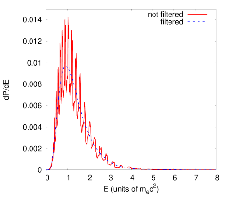
Figure 1: Positron energy spectra for the U$-$U head-on collision at energy $E=740$ MeV. The dashed (blue) line corresponds to the results obtained with the filtering procedure and solid (red) one denotes the values obtained without filter.

In Figs. 2 and 3, we present the obtained positron energy spectra for $b=0$ and $b=30$ fm. The corresponding monopole results from Ref. Maltsev_15 are also shown. It can be seen that the monopole and two-center spectra are very close to each other. It should be noted that the collision with $b=0$ is supercritical while the collision with $b=30$ fm is subcritical. However, all two-center spectra, as well as the monopole ones, have the same shape and do not exhibit any feature which can be associated with the spontaneous pair creation or the diving phenomenon.

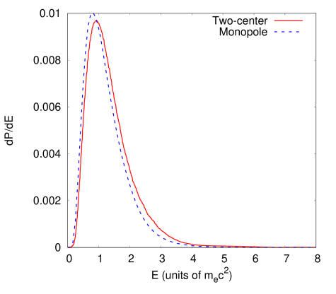
Figure 2: Positron energy spectrum for the U$-$U head-on collision at energy $E=740$ MeV. The solid (red) line corresponds to the results obtained with the full two-center potential and the dotted (blue) one denotes the values obtained in Ref. Maltsev_15 using the monopole approximation.

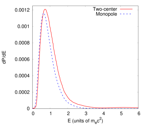
Figure 3: Positron energy spectrum for the U$-$U collision with the impact parameter $b=30$ fm at energy $E=740$ MeV. The solid (red) line corresponds to the results obtained with the full two-center potential and the dotted (blue) one denotes the values obtained in Ref. Maltsev_15 using the monopole approximation.

IV CONCLUSION

In the present work, we further evolved our method for calculation of pair production in low-energy ion collisions beyond the monopole approximation proposed in Ref. Maltsev_17 . Now this technique allows us to calculate the total pair-production probabilities, including the free-free ones, and the positron energy spectra in low-energy heavy-ion collisions.

Using the developed method we calculated pair production in collisions of bare uranium nuclei at energy near the Coulomb barrier. The obtained results were compared with the corresponding values from Ref. Maltsev_15 calculated in the monopole approximation. It was found that the effects beyond the monopole approximation are significant for free-free pair production. However, the bound-free pairs dominate in the two-center case as well as in the monopole one. For small values of the impact parameter the monopole results for the total pair-production probability are quite close to the two-center ones, but the difference increases with increasing the impact parameter.

The positron energy spectra calculated with the full two-center potential are very similar to the monopole ones. They do not exhibit any features that can be associated to the spontaneous pair production. This observation supports the conclusion of Refs. Reinhardt_81 ; Muller_88 ; Maltsev_15 that no direct evidence of the diving phenomenon can be found in the positron energy spectra. However, the methods beyond the monopole approximation make it possible to study the more detailed characteristics of the process under consideration. For instance, only the two-center methods allow one to calculate the angular-resolved energy distribution. Therefore these investigations open new opportunities for searching the scenarios for indirect detection of the diving phenomenon.

References

- (1) I. Pomeranchuk and J. Smorodinsky, J. Phys. USSR 9, 97 (1945).
- (2) S. S. Gershtein and Y. B. Zeldovich, Zh. Eksp. Teor. Fiz. 57, 654 (1969) [Sov. Phys. JETP 30, 358 (1970)].
- (3) W. Pieper and W. Greiner, Z. Phys. 218, 327 (1969).
- (4) Y. B. Zeldovich and V. S. Popov, Sov. Phys. Usp. 14, 673 (1972).
- (5) W. Greiner, B. Müller, and J. Rafelski, Quantum Electrodynamics of Strong Fields, (Springer-Verlag, Berlin, 1985).
- (6) U. Müller-Nehler and G. Soff, Phys. Rep. 246, 101 (1994).
- (7) S. I. Godunov, B. Machet, and M. I. Vysotsky, Eur. Phys. J. C 77, 782 (2017).
- (8) A. Gumberidze, Th. Stöhlker, H. F. Beyer, F. Bosch, A. Bräuning-Demian, S. Hagmann, C. Kozhuharov, Th. Kühl, R. Mann, P. Indelicato, W. Quint, R. Schuch, and A. Warczak, Nucl. Instrum. Methods Phys. Res. B 267, 248 (2009).
- (9) G. M. Ter-Akopian, W. Greiner, I. N. Meshkov, Y. T. Oganessian, J. Reinhardt, and G. V. Trubnikov, Int. J. Mod. Phys. E 24, 1550016 (2015).
- (10) X. Ma, W. Q. Wen, S. F. Zhang, D. Y. Yu, R. Cheng, J. Yang, Z. K. Huang, H. B. Wang, X. L. Zhu, X. Cai, Y. T. Zhao, L. J. Mao, J. C. Yang, X. H. Zhou, H. S. Xu, Y. J. Yuan, J. W. Xia, H. W. Zhao, G. Q. Xiao, and W. L. Zhan, Nucl. Instrum. Methods Phys. Res., Sect. B 408, 169 (2017).
- (11) S. S. Gershtein and V. S. Popov, Lett. Nuovo Cimento 6, 593 (1973).
- (12) V. S. Popov, Zh. Eksp. Teor. Fiz. 65, 35 (1973) [Sov. Phys. JETP 38, 18 (1974)].
- (13) H. Peitz, B. Müller, J. Rafelski, and W. Greiner, Lett. Nuovo Cimento 8, 37 (1973).
- (14) R. N. Lee and A. I. Milstein, Phys. Lett. B 8, 340 (2016).
- (15) I. B. Khriplovich, JETP Lett. 100, 494 (2014).
- (16) I. B. Khriplovich, Int. J. Mod. Phys. A 31, 1645035 (2016).
- (17) I. B. Khriplovich, Eur. Phys. J. Plus 132, 61 (2017).
- (18) J. Reinhardt, B. Müller, and W. Greiner, Phys. Rev. A 24, 103 (1981).
- (19) U. Müller, T. de Reus, J. Reinhardt, B. Müller, W. Greiner, and G. Soff, Phys. Rev. A 37, 1449 (1988).
- (20) E. Ackad and M. Horbatsch, J. Phys.: Conf. Ser. 88, 012017 (2007).
- (21) E. Ackad and M. Horbatsch, Phys. Rev. A 78, 062711 (2008).
- (22) I. A. Maltsev, V. M. Shabaev, I. I. Tupitsyn, A. I. Bondarev, Y. S. Kozhedub, G. Plunien, and Th. Stöhlker, Phys. Rev. A 91, 032708 (2015).
- (23) A. I. Bondarev, I. I. Tupitsyn, I. A. Maltsev, Y. S. Kozhedub, and G. Plunien, Eur. Phys. J. D 69, 110 (2015).
- (24) I. A. Maltsev, V. M. Shabaev, I. I. Tupitsyn, Y. S. Kozhedub, G. Plunien, and Th. Stöhlker, Nucl. Instrum. Methods Phys. Res. B 408, 97 (2017).
- (25) R. V. Popov, A. I. Bondarev, Y. S. Kozhedub, I. A. Maltsev, V. M. Shabaev, I. I. Tupitsyn, X. Ma, G. Plunien, and Th. Stöhlker, Eur. Phys. J. D 72, 115 (2018).
- (26) I. I. Tupitsyn, Y. S. Kozhedub, V. M. Shabaev, G. B. Deyneka, S. Hagmann, C. Kozhuharov, G. Plunien, and Th. Stöhlker, Phys. Rev. A 82, 042701 (2010).
- (27) E. B. Rozenbaum, D. A. Glazov, V. M. Shabaev, K. E. Sosnova, and D. A. Telnov, Phys. Rev. A 89, 012514 (2014).
- (28) E. S. Fradkin, D. M. Gitman, and S. M. Shvartsman, Quantum Electrodynamics with Unstable Vacuum, (Springer-Verlag, Berlin, 1991).
- (29) J. Crank and P. Nicolson, Proc. Cambridge Philos. Soc. 43, 50 (1947).
- (30) P. Joly and G. Meurant, Numer. Algorithms 4, 379 (1993).
- (31) X. S. Li and M. Shao, ACM Trans. Math. Software 37, 43 (2011).